Weighted SPICE: A Unifying Approach for Hyperparameter-Free Sparse Estimation

Abstract

In this paper we present the SPICE approach for sparse parameter estimation in a framework that unifies it with other hyperparameter-free methods, namely LIKES, SLIM and IAA. Specifically, we show how the latter methods can be interpreted as variants of an adaptively reweighted SPICE method. Furthermore, we establish a connection between SPICE and the $\ell_{1}$-penalized LAD estimator as well as the square-root LASSO method. We evaluate the four methods mentioned above in a generic sparse regression problem and in an array processing application.

I Introduction

During the past two decades, sparse parameter estimation for the ubiquitous linear model

$$\boldsymbol{y}=\boldsymbol{B}\boldsymbol{x}+\boldsymbol{e}\in\mathbb{C}^{N},\quad\boldsymbol{B}\in\mathbb{C}^{N\times M}$$ (1)

has become an important problem in signal processing, statistics and machine learning [1, 2, 3], with applications ranging from spectral analysis and direction-of-arrival estimation to magnetic resonance imaging and biomedical analysis [4, 5, 6, 7]. In this model $\boldsymbol{x}\in\mathbb{C}^{M}$ denotes the unknown sparse parameter vector and $\boldsymbol{y}\in\mathbb{C}^{N}$ is the vector of observations with typically $M\gg N$. The matrix of regressors $\boldsymbol{B}$ is assumed to be given and the unknown noise $\boldsymbol{e}$ is assumed to have zero mean. For $M>N$, the problem is ill-posed, unless the knowledge about the sparsity of $\boldsymbol{x}$ is exploited.

Exploiting sparsity also enables one to tackle nonlinear estimation problems. Consider, for example, a nonlinear model which consists of the superposition of an unknown number of mode vectors

$$\boldsymbol{y}=\sum_{i}\boldsymbol{h}(\tilde{\boldsymbol{\theta}}_{i})\tilde{x}_{i}+\boldsymbol{e},$$

where $\boldsymbol{h}(\tilde{\boldsymbol{\theta}})$ is a given function of unknown parameters $\tilde{\boldsymbol{\theta}}_{i}\in\Theta$. Each mode has an amplitude $\tilde{x}_{i}$. This model is relevant to spectral analysis and related applications. By griding the parameter space $\Theta$ using a sufficiently large number of points $\{\boldsymbol{\theta}_{k}\}^{M}_{k=1}$, we can approximate the nonlinear model by means of a dictionary of mode vectors evaluated at the fixed grid points $\boldsymbol{B}=[\boldsymbol{h}(\boldsymbol{\theta}_{1})\>\cdots\>\boldsymbol{h}(\boldsymbol{\theta}_{M})]$ such that $\boldsymbol{x}=[x_{1}\>\cdots\>x_{M}]^{\top}$ becomes a sparse vector and (1) applies. Identification of a nonzero component $x_{k}$ therefore concomitantly identifies the corresponding gridpoint $\boldsymbol{\theta}_{k}$ which becomes an estimate of the nonlinear parameter. Another example, that appears in applications of machine learning and statistics, is finding a general input-output mapping

$$y_{i}=h(\boldsymbol{\theta}_{i})+e_{i},$$

from data $\{\boldsymbol{\theta}_{i},y_{i}\}^{N}_{i=1}$. The nonlinear mapping is modeled by a sparse linear combination of kernel functions, $h(\boldsymbol{\theta}_{i})=\sum^{N}_{j=1}k(\boldsymbol{\theta}_{i},\boldsymbol{\theta}_{j})x_{j}$, where $\{x_{j}\}$ denote the expansion coefficients [8]. Thus the sparse linear model (1) applies and identification of the nonlinear mapping can be posed as a sparse parameter estimation problem, where the $ij$th element of $\boldsymbol{B}$ is given by the kernel function $k(\boldsymbol{\theta}_{i},\boldsymbol{\theta}_{j})$.

Many popular sparse estimation methods are based on regularizing the least-squares method by penalizing a norm of the parameter vector $\boldsymbol{x}$, in an attempt to strike a balance between data fidelity and parameter sparsity. While such sparsifying methods can estimate $\boldsymbol{x}$ in highly underdetermined scenarios, most of them require the careful selection of user-defined regularization hyperparameters [9, 10, 11, 12], cf. [13] for a critical discussion.

Recently, a sparse iterative covariance-based estimation method (Spice) was proposed which does not require any hyperparameters, yet has good statistical properties [14, 15, 16]. In this tutorial paper:

• We set out to derive four different hyperparameter-free methods in a unifying Spice-like manner: the methods are Spice, Likes, Slim and Iaa [16, 17, 18]. In the process we provide insights into these methods, and derive new versions of each of them.

• Furthermore, we establish the connection between Spice and $\ell_{1}$-penalized Lad as well as the square-root Lasso methods [19, 20].

• Finally, we evaluate the four methods in two different scenarios: a generic sparse regression problem and a direction-of-arrival estimation application.

Notation: Matrices, vectors and scalars are distinguished by $\boldsymbol{A}$, $\boldsymbol{a}$ and $a$, respectively. $\text{Re}\{a\}$ denotes the real part of $a$. Defined variables are signified by $\triangleq$. $\boldsymbol{A}^{1/2}$ is a matrix square-root of $\boldsymbol{A}$ and $\boldsymbol{A}^{-1/2}$ is its inverse. $\boldsymbol{A}\otimes\boldsymbol{B}$ and $\boldsymbol{A}\odot\boldsymbol{B}$ denote the Kronecker and Khatri-Rao matrix products. $\boldsymbol{A}^{\top}$ and $\boldsymbol{A}^{*}$ denote the transpose and Hermitian transpose of $\boldsymbol{A}$. $\text{vec}(\boldsymbol{A})$ is the column-wise vectorization of $\boldsymbol{A}$. $\|\cdot\|_{1}$, $\|\cdot\|_{2}$ and $\|\cdot\|_{F}$ are the $\ell_{1}$, $\ell_{2}$ and Frobenius norms, and $\|\cdot\|_{0}$ denotes the $\ell_{0}$ ‘quasi-norm’ which equals the number of nonzero entries of a vector. $\text{tr}\{\boldsymbol{A}\}$ and $|\boldsymbol{A}|$ denote the trace and determinant of a square matrix $\boldsymbol{A}$. We use $\text{diag}(d_{1},\dots,d_{N})$ or $\text{diag}(\boldsymbol{d})$ to compactly denote a diagonal matrix with entries from $\boldsymbol{d}$. $\boldsymbol{A}\succeq\boldsymbol{B}$ signifies the Löwner order between Hermitian matrices $\boldsymbol{A}$ and $\boldsymbol{B}$. The Kronecker delta is denoted by $\delta_{jk}$. The proper complex Gaussian distribution with mean $\boldsymbol{\mu}$ and covariance matrix $\boldsymbol{\Sigma}$ is denoted $\mathcal{CN}(\boldsymbol{\mu},\boldsymbol{\Sigma})$. The probability of event $E$ is written as $\Pr\{E\}$.

Abbreviations: If and only if (iff). Subject to (s.t.). With respect to (w.r.t.). Identically and independently distributed (IID). Signal-to-noise ratio (SNR). Mean square error (MSE). Linear minimum mean square error (LMMSE). Least squares (LS). Second-order cone program (SOCP). Direction-of-arrival (DOA). Uniform linear array (ULA). Least absolute deviation (Lad). Least absolute shrinkage and selection operator (Lasso). Focal underdetermined system solver (Focuss). Sparse iterative covariance-based estimation (Spice). Likelihood-based estimation of sparse parameters (Likes). Sparse learning via iterative minimization (Slim). Iterative adaptive approach (Iaa).

II Brief review of the basic Spice approach

Spice was introduced as a covariance fitting approach in [14, 15, 16]. In what follows we consider the one-snapshot case of (1), but the method is easily extended to the multisnapshot case as we show in Appendix A. Consider the following ‘model’ for the covariance matrix of the data vector $\boldsymbol{y}$:

$$\begin{split}\boldsymbol{R}&=\boldsymbol{B}\begin{bmatrix}p_{1}&&0\\ &\ddots&\\ 0&&p_{M}\end{bmatrix}\boldsymbol{B}^{*}+\begin{bmatrix}p_{M+1}&&0\\ &\ddots&\\ 0&&p_{M+N}\end{bmatrix}\\ &=\boldsymbol{A}\boldsymbol{P}\boldsymbol{A}^{*}\in\mathbb{C}^{N\times N},\end{split}$$ (2)

where

$$\boldsymbol{A}\triangleq[\boldsymbol{B}\;\boldsymbol{I}_{N}],\quad\boldsymbol{P}\triangleq\text{diag}(\boldsymbol{p}),$$

and where $\boldsymbol{A}=[\boldsymbol{a}_{1}\>\boldsymbol{a}_{2}\>\cdots\>\boldsymbol{a}_{M+N}]\in\mathbb{C}^{N\times(M+N)}$ and $\boldsymbol{p}\triangleq[p_{1},\dots,p_{M+N}]^{\top}\in\mathbb{R}^{M+N}_{+}$. The covariance matrix $\boldsymbol{R}(\boldsymbol{p})$ is a function of the parameters $\{p_{k}\}$ which can be interpreted as the variances of $\{x_{k}\}$ and $\{e_{k}\}$. In the next section, we will discuss the covariance model (2) in more detail. While it appears to assume that $\{x_{k},e_{k}\}$ are uncorrelated, this should not be interpreted as a restriction, as will be explained.

In the spectral analysis applications of sparse parameter estimation, the main goal is to estimate $\{p_{k}\}$. In most of the other applications, the goal is the estimation of $\boldsymbol{x}$. Even in the latter case, there exists a class of methods (that includes those discussed here) which first obtain estimates $\{\hat{p}_{k}\}$ of $\{p_{k}\}$ and then, if desired, estimate $\boldsymbol{x}$ via the usual LMMSE estimator formula [21]:

$$\hat{x}_{k}=\hat{p}_{k}\boldsymbol{a}^{*}_{k}\widehat{\boldsymbol{R}}^{-1}\boldsymbol{y},\>k=1,\dots,M,$$ (3)

where $\widehat{\boldsymbol{R}}=\boldsymbol{A}\widehat{\boldsymbol{P}}\boldsymbol{A}^{*}$. As we show in the next sections, this estimate also occurs naturally within an augmented version of the Spice approach. An alternative is to use the Capon formula [22]:

$$\hat{x}_{k}=\frac{\boldsymbol{a}^{*}_{k}\widehat{\boldsymbol{R}}^{-1}\boldsymbol{y}}{\boldsymbol{a}^{*}_{k}\widehat{\boldsymbol{R}}^{-1}\boldsymbol{a}_{k}},\>k=1,\dots,M.$$ (4)

In general one can expected (4) to be a less biased estimate than (3), but (3) to have a smaller MSE. Interestingly, if the same $\widehat{\boldsymbol{P}}$ is used in both (3) and (4) then:

$$|\hat{x}_{k}|_{(3)}\leq|\hat{x}_{k}|_{(4)}.$$ (5)

In particular this means that the estimate (3) of $\boldsymbol{x}$ is always sparser than (4). This fact follows from the following simple result:

Lemma 1.

$$\hat{p}_{k}\leq\frac{1}{\boldsymbol{a}^{*}_{k}\widehat{\boldsymbol{R}}^{-1}\boldsymbol{a}_{k}}.\>$$ (6)

The proof of this lemma, as well as of the subsequent ones, can be found in Appendix B.

If a $K$-sparse estimate of $\boldsymbol{x}$ is desired, that is an estimate $\{\hat{x}_{k}\}$ where only $K$ elements are nonzero, then we can apply the LS method to (1) where we retain only the columns of $\boldsymbol{B}$ whose indices correspond to the $K$ largest peaks of $\{\hat{p}_{k}\}^{M}_{k=1}$.

Spice estimates $\{p_{k}\}$ by minimizing the following covariance fitting criterion:

$$\begin{split}\|\boldsymbol{R}^{-1/2}(\boldsymbol{y}\boldsymbol{y}^{*}-\boldsymbol{R})\|^{2}_{F}&=\text{tr}\{(\boldsymbol{y}\boldsymbol{y}^{*}-\boldsymbol{R})\boldsymbol{R}^{-1}(\boldsymbol{y}\boldsymbol{y}^{*}-\boldsymbol{R})\}\\ &=\|\boldsymbol{y}\|^{2}_{2}\boldsymbol{y}^{*}\boldsymbol{R}^{-1}\boldsymbol{y}+\text{tr}\{\boldsymbol{R}\}+\text{const.},\end{split}$$ (7)

or equivalently,

$$\boldsymbol{y}^{*}\boldsymbol{R}^{-1}\boldsymbol{y}+\frac{1}{\|\boldsymbol{y}\|^{2}_{2}}\sum^{M+N}_{k=1}w_{k}p_{k},\quad w_{k}=\|\boldsymbol{a}_{k}\|^{2}_{2}.$$ (8)

Next we note the following result:

Lemma 2.

Let

$$\hat{\boldsymbol{p}}=\operatorname*{arg\,min}_{\boldsymbol{p}}\>g(\boldsymbol{p}),\;g(\boldsymbol{p})=\boldsymbol{y}^{*}\boldsymbol{R}^{-1}(\boldsymbol{p})\boldsymbol{y}+c^{2}\sum^{M+N}_{k=1}w_{k}p_{k},$$

where $\>c>0$, and let

$$\hat{\bar{\boldsymbol{p}}}=\operatorname*{arg\,min}_{\bar{\boldsymbol{p}}}\>f(\bar{\boldsymbol{p}}),\;f(\bar{\boldsymbol{p}})=\boldsymbol{y}^{*}\boldsymbol{R}^{-1}(\bar{\boldsymbol{p}})\boldsymbol{y}+\sum^{M+N}_{k=1}w_{k}\bar{p}_{k}.$$

Then

$$\hat{\bar{\boldsymbol{p}}}=c\hat{\boldsymbol{p}}.$$

Note also that a uniform scaling of $\{\hat{p}_{k}\}$ leaves $\{\hat{x}_{k}\}$ unchanged whether using LMMSE, Capon or LS. It follows from these observations that the constant factor $\|\boldsymbol{y}\|^{2}_{2}$ in (8) can be omitted. Thus we can reformulate the Spice criterion as:

$$\min_{\{p_{k}\}}\;\boldsymbol{y}^{*}\boldsymbol{R}^{-1}\boldsymbol{y}+\sum^{M+N}_{k=1}w_{k}p_{k}.$$ (9)

When $\|\boldsymbol{a}_{k}\|_{2}\equiv\text{const}.$, the weights in (9) can be replaced by 1’s.

The problem in (9) is convex, namely an SOCP [15], and hence it can be solved globally [23]. Rather than solving it by an off-the-shelves SOCP code, the following iterative cyclic minimizer, which monotonically decreases (9) at each iteration and converges globally [14, 15], was found to be preferable from a computational standpoint:

$$\hat{p}^{i+1}_{k}=\hat{p}^{i}_{k}|\boldsymbol{a}^{*}_{k}\widehat{\boldsymbol{R}}^{-1}_{i}\boldsymbol{y}|/\sqrt{w_{k}},\quad(\text{{Spice}}_{\text{a}})$$ (10)

where $\quad k=1,2,\dots,M+N$ and $\widehat{\boldsymbol{R}}_{i}=\boldsymbol{A}\text{diag}(\hat{\boldsymbol{p}}^{i})\boldsymbol{A}^{*}$ denotes the covariance matrix estimate at iteration $i$; we use a subindex ‘a’ for the Spice algorithm in (10) to differentiate it from a variation that will be presented later on, see Section IV below.

We remark on the fact that we have allowed the noise $\boldsymbol{e}$ to have different powers, say $\sigma^{2}_{1}=p_{M+1}$, $\sigma^{2}_{2}=p_{M+2},\dots,\sigma^{2}_{N}=p_{M+N}$, in different data samples for three reasons:

• notational simplicity (it allows treating the noise powers similarly to $\{p_{k}\}^{M}_{k=1}$ and not differently as is the case when the condition $\sigma^{2}_{k}\equiv\sigma^{2},\forall k$, is enforced).

• generality (in some applications, $\sigma^{2}_{1},\sigma^{2}_{2},\dots,\sigma^{2}_{N}$, may well be different from one another).

• even if the noise powers are uniform, $\sigma^{2}_{k}\equiv\sigma^{2}$, $\forall k$, but we either do not know that or prefer not to impose this condition, Spice with different noise powers works well. Indeed, the degradation of accuracy compared with that achieved by imposing $\sigma^{2}_{k}\equiv\sigma^{2}$, $\forall k$, is not significant – we explain why this is so in the next section. On the other hand, if we are sure that $\sigma^{2}_{k}\equiv\sigma^{2}$, $\forall k$, and want to enforce this condition, then we can do so with only some minor modifications of the algorithms (see [14, 15, 16] and Appendix C).

Finally, we note that the form of Spice${}_{\text{a}}$ iteration, (10), is similar to that associated with Focuss [24]; the main difference between the two methods lies in the way the noise powers are treated: Focuss assumes that the noise powers are identical and given (possibly estimated by some other method), whereas Spice does not make this restrictive assumption.

III On the covariance model and the link of Spice to $\ell_{1}$-penalized Lad

There are several important questions about the covariance model in (2):

1. Assume that $\boldsymbol{x}$ and $\boldsymbol{e}$ are drawn from correlated distributions (i.e. distributions whose covariance matrices are not diagonal). Then will Spice, and the other estimation methods discussed later, still work despite seemingly relying on the diagonal covariance matrix in (2)? Note that in the Bayesian approach to sparse estimation (see e.g. [25]), (2) is viewed as a ‘prior information’ – however this does not offer any satisfactory answer to the above equation, as priors are not ‘forgotten’ in problems with many more unknowns than data samples (i.e. $M\gg N)$, as in the case considered here.

2. In fact what do $\{\hat{p}_{k}\}$ estimate? Do they estimate $\{|x_{k}|^{2}\}$?

3. If indeed $\sigma^{2}_{k}\equiv\sigma^{2}$, $\forall k$, do we significantly degrade the accuracy by using a nonuniform noise power model as in (2)?

4. Is (2) a unique description, i.e. for a given $\boldsymbol{P}$ can we find a $\bar{\boldsymbol{P}}\neq\boldsymbol{P}$ such that $\boldsymbol{A}\boldsymbol{P}\boldsymbol{A}^{*}=\boldsymbol{A}\bar{\boldsymbol{P}}\boldsymbol{A}^{*}$?

We will provide answers to questions a)-c) by establishing the connection between the Spice criterion in (9) and the $\ell_{1}$-penalized Lad criterion. Then we will address the question in d) by means of a separate analysis.

To understand the role of $\boldsymbol{p}$ in the estimation of $\boldsymbol{x}$, we rewrite the criterion in (9) in terms of the original model (1), with the help of the following result.

Lemma 3.

Let

$$\boldsymbol{S}=\begin{bmatrix}p_{M+1}&&0\\ &\ddots&\\ 0&&p_{M+N}\end{bmatrix},\;\boldsymbol{\Pi}=\begin{bmatrix}p_{1}&&0\\ &\ddots&\\ 0&&p_{M}\end{bmatrix}.$$

Then

$$\min_{\boldsymbol{x}}\>(\boldsymbol{y}-\boldsymbol{B}\boldsymbol{x})^{*}\boldsymbol{S}^{-1}(\boldsymbol{y}-\boldsymbol{B}\boldsymbol{x})+\sum^{M}_{k=1}|x_{k}|^{2}/p_{k}=\boldsymbol{y}^{*}\boldsymbol{R}^{-1}\boldsymbol{y}$$ (11)

and the minimum value occurs at

$$\hat{\boldsymbol{x}}=\boldsymbol{\Pi}\boldsymbol{B}^{*}\boldsymbol{R}^{-1}\boldsymbol{y}.$$ (12)

It follows from the above lemma that the minimizer of the Spice criterion in (9) can also be obtained by minimizing the following function (w.r.t. both $\boldsymbol{x}$ and $\boldsymbol{p}$):

$$\sum^{N}_{k=1}|y_{k}-\boldsymbol{b}^{*}_{k}\boldsymbol{x}|^{2}/p_{M+k}+\sum^{M}_{k=1}|x_{k}|^{2}/p_{k}\;+\sum^{M+N}_{k=1}w_{k}p_{k},$$ (13)

where $\boldsymbol{b}^{*}_{k}$ denotes the $k$th row of $\boldsymbol{B}$. Minimization of (13) w.r.t. $\{p_{k}\}$ yields:

$$\begin{split}p_{k}&=|x_{k}|/\sqrt{w_{k}},\;k=1,\dots,M\\ p_{M+k}&=|y_{k}-\boldsymbol{b}^{*}_{k}\boldsymbol{x}|/\sqrt{w_{M+k}},\;k=1,\dots,N.\end{split}$$ (14)

Insertion of (14) into (13) gives:

$$\|\boldsymbol{W}^{1/2}_{1}(\boldsymbol{y}-\boldsymbol{B}\boldsymbol{x})\|_{1}+\left\|\boldsymbol{W}^{1/2}_{2}\boldsymbol{x}\right\|_{1},$$ (15)

where $\boldsymbol{W}_{1}=\text{diag}(w_{M+1},\dots,w_{M+N})$ and $\boldsymbol{W}_{2}=\text{diag}(w_{1},\dots,w_{M})$; this is recognized as a (weighted) $\ell_{1}$-penalized Lad criterion [19].

The above analysis has several implications, some for Lad:

• The $\ell_{1}$-penalized Lad estimate of $\boldsymbol{x}$ can be obtained using the Spice${}_{\text{a}}$ algorithm, (10), to estimate $\{p_{k}\}$ and then get $\hat{\boldsymbol{x}}$ from (12) (note that (12) is identical to (3)). For the complex-valued data case, Spice can be expected to be faster than other convex programming techniques that are used to get $\hat{\boldsymbol{x}}$ from (15) directly.

• If the condition $\sigma^{2}_{1}=\sigma^{2}_{2}=\cdots=\sigma^{2}_{N}$ is enforced, then the Spice approach was shown in [26, 27] to be equivalent to the square-root Lasso method of [20] (see also Appendix C for a more direct proof of this equivalance result). This fact establishes an interesting connection between square-root Lasso and $\ell_{1}$-penalized Lad.

and some for Spice:

• The Spice estimates $\{\hat{p}_{k}\}$ of $\{p_{k}\}$ are not estimates of $|x_{k}|^{2}$ and $|e_{k}|^{2}$ but of (scaled versions of) the square-roots of these quantities. However, when $w_{k}$ is an estimate of $1/p_{k}$, or a quantity related to $1/p_{k}$ (see Section IV), then it follows from (14) that $\{\hat{p}_{k}\}$ estimates $|x_{k}|^{2}$.

• Spice will still work even if the $\{x_{k}\}$ and $\{e_{k}\}$ in (1) are drawn from correlated distributions; indeed, when Spice is viewed from the perspective of its equivalence with $\ell_{1}$-penalized Lad (or square-root Lasso), its performance does not depend significantly on the way $\boldsymbol{x}$ and $\boldsymbol{e}$ were generated because the performance of the $\ell_{1}$-penalized Lad or square-root Lasso is not strongly dependent on that [19, 20]; in this light, $\{p_{k}\}$ and the ‘covariance model’ in (2) can be viewed as being nothing but instruments employed to achieve the equivalence proven above; and hence not for necessarily providing a true description of the data covariance matrix. Similarly, by not imposing the condition $\sigma^{2}_{1}=\sigma^{2}_{2}=\cdots=\sigma^{2}_{N}$, when this was known to be true, we basically do nothing but choose to use $\ell_{1}$-penalized Lad in lieu of square-root Lasso, and the difference in accuracy between the latter methods is usually not significant.

In the above discussion we have provided answers to questions a)-c). Next, we turn our attention to question d). The parameterization/description (2) of $\boldsymbol{R}$ is unique iff there is no diagonal matrix $\boldsymbol{Q}=\text{diag}(\boldsymbol{q})\neq\boldsymbol{0}$ (where $\boldsymbol{q}\in\mathbb{R}^{M+N}$) which is such that:

$$\boldsymbol{A}\boldsymbol{Q}\boldsymbol{A}^{*}=\boldsymbol{0}$$ (16)

and

$$\boldsymbol{P}+\boldsymbol{Q}\succeq\boldsymbol{0},$$ (17)

Equation (16) can be re-written as:

$$\begin{split}\text{vec}(\boldsymbol{A}\boldsymbol{Q}\boldsymbol{A}^{*})&=\text{vec}\left(\sum^{M+N}_{k=1}q_{k}\boldsymbol{a}_{k}\boldsymbol{a}^{*}_{k}\right)\\ &=[\boldsymbol{a}^{*\top}_{1}\otimes\boldsymbol{a}_{1}\>\cdots\>\boldsymbol{a}^{*\top}_{M+N}\otimes\boldsymbol{a}_{M+N}]\boldsymbol{q}=\boldsymbol{0},\end{split}$$

i.e., equivalently,

$$(\boldsymbol{A}^{*\top}\odot\boldsymbol{A})\boldsymbol{q}=\boldsymbol{0}.$$ (18)

Also, for easy reference, we can write (17) as $\boldsymbol{p}+\boldsymbol{q}\geq\boldsymbol{0}$. In the analysis of (18), the rank of the matrix $\widetilde{\boldsymbol{A}}\triangleq\boldsymbol{A}^{*\top}\odot\boldsymbol{A}$ clearly is an essential factor:

1. Assume that $M<N$ (i.e. $M+N<2N$) and that any $N$ columns of $\boldsymbol{A}$ are linearly independent. Then $\text{rank}(\widetilde{\boldsymbol{A}})=M+N$ [28] and thus (18) implies $\boldsymbol{q}=\boldsymbol{0}$, which means that the description (2) of $\boldsymbol{R}$ is unique.

2. If $M+N<N^{2}$, then $\widetilde{\boldsymbol{A}}$ has full rank (equal to $M+N$) for almost any matrix $\boldsymbol{A}$ (assumed to be drawn from a continuous distribution) [29] and hence (2) is generically unique.

3. For $M+N>N^{2}$, $\text{rank}(\widetilde{\boldsymbol{A}})<M+N$ and there exists $\boldsymbol{q}\neq\boldsymbol{0}$ that satisfy (18). In this scenario one must consider two cases. Let $r$ be the maximum integer such that any $r$ columns of $\tilde{\boldsymbol{A}}$ are linearly independent. Then, if $\|\boldsymbol{p}\|_{0}>r$, (2) is not unique, whereas if $\|\boldsymbol{p}\|_{0}\leq r$ then (2) may be unique or nonunique depending on the instance of $\boldsymbol{A}$ and $\boldsymbol{p}$ under consideration. To see this, let $\bar{\boldsymbol{A}}$ denote the matrix made from the columns of $\tilde{\boldsymbol{A}}$ corresponding to the nonzero elements of $\boldsymbol{p}$. When $\|\boldsymbol{p}\|_{0}>r$ there exists a vector $\bar{\boldsymbol{q}}\neq\boldsymbol{0}$ such that $\bar{\boldsymbol{A}}\bar{\boldsymbol{q}}=\boldsymbol{0}$. By appending $\bar{\boldsymbol{q}}$ with zeros we can therefore form a vector $\boldsymbol{q}$ that fulfills both $\tilde{\boldsymbol{A}}\varepsilon\boldsymbol{q}=\boldsymbol{0}$ and $\boldsymbol{p}+\varepsilon\boldsymbol{q}\geq 0$, for a sufficiently small $\varepsilon$. On the other hand, when $\|\boldsymbol{p}\|_{0}\leq r$ then such a vector $\boldsymbol{q}$ in the nullspace of $\tilde{\boldsymbol{A}}$ may or may not satisfy (17) depending on whether the signs of the coefficients which do not belong to the support of $\boldsymbol{p}$ are all the same.

IV Likes, Slim, Iaa (and new versions thereof) as (re)weighted Spice

Consider the Spice fitting criterion in (9) with general weights $\{w_{k}>0\}$ (possibly different than the weights in (9)). For fixed weights, (9) is a convex function of $\{p_{k}\}$, which can be globally minimized, for example, by the algorithm in (10). In the following we will derive (10) by using a gradient approach that is simpler than the cyclic minimization approach employed in [14, 15, 16]. The gradient approach is also more flexible in that it suggests alternatives to (10) which may be interesting in their own right.

IV-A Weighted Spice

The derivative of (9) w.r.t. $p_{k}$ is equal to

$$-\boldsymbol{y}^{*}\boldsymbol{R}^{-1}\frac{\partial\boldsymbol{R}}{\partial p_{k}}\boldsymbol{R}^{-1}\boldsymbol{y}+w_{k}=-|\boldsymbol{a}^{*}_{k}\boldsymbol{R}^{-1}\boldsymbol{y}|^{2}+w_{k}.$$ (19)

Consequently, the $(i+1)$th iteration of a gradient algorithm (with variable step length) applied to (9) is given by:

$$\hat{p}^{i+1}_{k}=\hat{p}^{i}_{k}-\rho^{i}_{k}(w_{k}-|\boldsymbol{a}^{*}_{k}\widehat{\boldsymbol{R}}^{-1}_{i}\boldsymbol{y}|^{2}),$$ (20)

where $\widehat{\boldsymbol{R}}_{i}$ is made from $\{\hat{p}^{i}_{k}\}$, as before, and the step size $\rho^{i}_{k}$ must be non-negative

$$\rho^{i}_{k}\geq 0.$$ (21)

Because $\{p_{k}\geq 0\}$ by definition, we shall also choose $\rho^{i}_{k}$ such that:

$$\hat{p}^{i}_{k}\geq 0\>\Rightarrow\>\hat{p}^{i+1}_{k}\geq 0.$$ (22)

Let us choose

$$\rho^{i}_{k}=\frac{\hat{p}^{i}_{k}}{w_{k}+w^{1/2}_{k}|\boldsymbol{a}^{*}_{k}\widehat{\boldsymbol{R}}^{-1}_{i}\boldsymbol{y}|}$$ (23)

which satisfies (21). A simple calculation gives:

$$\begin{split}\hat{p}^{i+1}_{k}&=\frac{\hat{p}^{i}_{k}w_{k}+\hat{p}^{i}_{k}w^{1/2}_{k}|\boldsymbol{a}^{*}_{k}\widehat{\boldsymbol{R}}^{-1}_{i}\boldsymbol{y}|-\hat{p}^{i}_{k}w_{k}+\hat{p}^{i}_{k}|\boldsymbol{a}^{*}_{k}\widehat{\boldsymbol{R}}^{-1}_{i}\boldsymbol{y}|^{2}}{w_{k}+w^{1/2}_{k}|\boldsymbol{a}^{*}_{k}\widehat{\boldsymbol{R}}^{-1}_{i}\boldsymbol{y}|}\\ &=\frac{\hat{p}^{i}_{k}|\boldsymbol{a}^{*}_{k}\widehat{\boldsymbol{R}}^{-1}_{i}\boldsymbol{y}|}{w^{1/2}_{k}},\end{split}$$

that is,

$$\hat{p}^{i+1}_{k}=\hat{p}^{i}_{k}|\boldsymbol{a}^{*}_{k}\widehat{\boldsymbol{R}}^{-1}_{i}\boldsymbol{y}|/w^{1/2}_{k}\quad(\text{{Spice}}_{\text{a}})$$ (24)

and thus (22) is satisfied too. Note that when $w_{k}=\|\boldsymbol{a}_{k}\|^{2}_{2}$, (24) is nothing but the Spice${}_{\text{a}}$ algorithm in equation (10), whose derivation above is more direct than the derivation in [14, 15, 16] which was based on cyclically minimizing an augmented criterion function.

As already mentioned, the gradient approach is also more flexible in the sense that $\rho^{i}_{k}$ in (20) can be chosen in several different ways than (23) to obtain alternative algorithms to (24). A particularly simple such choice (that satisfies (21)) is:

$$\rho^{i}_{k}=\hat{p}^{i}_{k}/w_{k}$$ (25)

which leads to

$$\hat{p}^{i+1}_{k}=\hat{p}^{i}_{k}|\boldsymbol{a}^{*}_{k}\widehat{\boldsymbol{R}}^{-1}_{i}\boldsymbol{y}|^{2}/w_{k}\quad(\text{{Spice}}_{\text{b}})$$ (26)

(therefore (22) is satisfied as well). When $w_{k}=\|\boldsymbol{a}_{k}\|^{2}_{2}$, (26) minimizes the same criterion as (24) and will therefore be referred to as Spice${}_{\text{b}}$. Both algorithms share the same stationary points, but they may have different rates of convergence. In particular observe that the step length in (23) is smaller than (25), when both are evaluated using the same $\{\hat{p}^{i}_{k}\}$.

In the next sections we will consider different choices of the weights than Spice’s, which will lead to other hyperparameter-free methods, namely Likes, Slim and Iaa. Unlike Spice, whose weights are constant, these algorithms use data-dependent weights that change with the iteration.

IV-B Likes

The current problem of estimating $\{p_{k}\}$ from $\boldsymbol{y}$ is not a standard one especially owing to the fact that $M+N$ = number of unknowns $\gg 2N$ = number of (real-valued) data. Even so, the analysis in [30], as well as data-whitening considerations, suggest that a possibly (statistically) better covariance matching criterion than (7) is the following one:

$$\|\boldsymbol{R}^{-1/2}(\boldsymbol{y}\boldsymbol{y}^{*}-\boldsymbol{R})\widehat{\boldsymbol{R}}^{-1/2}\|^{2}_{F},$$ (27)

where $\widehat{\boldsymbol{R}}$ is an available estimate of $\boldsymbol{R}$. A straightforward calculation shows that (27) can be re-written as:

$$\begin{split}&\text{tr}\left[(\boldsymbol{y}\boldsymbol{y}^{*}-\boldsymbol{R})\widehat{\boldsymbol{R}}^{-1}(\boldsymbol{y}\boldsymbol{y}^{*}-\boldsymbol{R})\boldsymbol{R}^{-1}\right]\\ &=(\boldsymbol{y}^{*}\widehat{\boldsymbol{R}}^{-1}\boldsymbol{y})(\boldsymbol{y}^{*}{\boldsymbol{R}}^{-1}\boldsymbol{y})+\text{tr}(\widehat{\boldsymbol{R}}^{-1}\boldsymbol{R})+\text{const.}\\ &=(\boldsymbol{y}^{*}\widehat{\boldsymbol{R}}^{-1}\boldsymbol{y})(\boldsymbol{y}^{*}{\boldsymbol{R}}^{-1}\boldsymbol{y})+\sum^{M+N}_{k=1}(\boldsymbol{a}^{*}_{k}\widehat{\boldsymbol{R}}^{-1}\boldsymbol{a}_{k})p_{k}+\text{const.}\end{split}$$ (28)

In view of Lemma 2 we can omit the constant factor $(\boldsymbol{y}^{*}\widehat{\boldsymbol{R}}^{-1}\boldsymbol{y})$ in (28), which leads to the following weighted Spice criterion:

$$\boldsymbol{y}^{*}{\boldsymbol{R}}^{-1}\boldsymbol{y}+\sum^{M+N}_{k=1}w_{k}p_{k},\quad w_{k}=(\boldsymbol{a}^{*}_{k}\widehat{\boldsymbol{R}}^{-1}\boldsymbol{a}_{k}).$$ (29)

Unlike Spice’s weights, which are data independent, the $\{w_{k}\}$ in (29) depend on the data (via $\widehat{\boldsymbol{R}}$). Note that $w_{k}$ in (29) can be interpreted as the Capon estimate of $1/p_{k}$ (see e.g. [22]). This means that the penalty term in (29) is an approximation of $\|\boldsymbol{p}\|_{0}$ rather than just being proportional to the $\ell_{1}$-norm of $\boldsymbol{p}$ as for Spice. It is well known that the $\ell_{0}$-(quasi)norm is the most sensible measure of the sparsity of a parameter vector because it is not dependent on the size of the elements of that vector, as is the $\ell_{1}$-norm (see, e.g., [31] for a general discussion on this aspect).

It follows from the above discussion that the weights in (29) are intuitively a more appealing choice than the Spice’s weights in (9). The data-dependent weights in (29) can be updated in the following way:

1. Fix $\widehat{\boldsymbol{R}}$ in $\{w_{k}\}$ and use (24) or (26) to minimize (29), or at least monotonically decrease this function for a pre-specified number of iterations.

2. Update $\widehat{\boldsymbol{R}}$ in (29), and the weights $\{w_{k}\}$, and go to step i).

This leads to the following iterative schemes:

$$\hat{p}^{i+1}_{k}=\hat{p}^{i}_{k}|\boldsymbol{a}^{*}_{k}\widehat{\boldsymbol{R}}^{-1}_{i}\boldsymbol{y}|/(\boldsymbol{a}^{*}_{k}\widehat{\boldsymbol{R}}^{-1}_{\ell}\boldsymbol{a}_{k})^{1/2},\quad(\text{{Likes}}_{\text{a}})$$ (30)

or, alternatively,

$$\hat{p}^{i+1}_{k}=\hat{p}^{i}_{k}|\boldsymbol{a}^{*}_{k}\widehat{\boldsymbol{R}}^{-1}_{i}\boldsymbol{y}|^{2}/(\boldsymbol{a}^{*}_{k}\widehat{\boldsymbol{R}}^{-1}_{\ell}\boldsymbol{a}_{k})\quad(\text{{Likes}}_{\text{b}}).$$ (31)

Initially, we set $\ell=0$, and the above updates are executed as follows:

1. Iterate for $i=\ell,\ell+1,\dots,\ell+m-1$, where $m$ is the number of iterations in which the weights are kept fixed.

2. Reset $\ell\leftarrow\ell+m$, and go to 1).

The algorithm in (30) is recognized as Likes [16], whereas the one in (31) is a new version. To distinguish between them we have designated them as Likes${}_{\text{a}}$ and Likes${}_{\text{b}}$, respectively. Because these algorithms update the weights in (29), they can only be interpreted as minimizers of the criterion in (29) using the weights obtained at convergence. This does not say much as to the convergence properties of (30) or (31), an aspect that will be addressed in the next section. Here we only note that the two iterative algorithms above clearly have the same stationary points. However, their rates of convergence to a stationary point may be different from one another.

IV-C Slim

Consider (29) with different weights:

$$w_{k}=1/\hat{p}_{k}.$$ (32)

The corresponding penalty term in (29) would then be a more direct approximation of $\|\boldsymbol{p}\|_{0}$ than when $w_{k}=\boldsymbol{a}^{*}_{k}\widehat{\boldsymbol{R}}^{-1}\boldsymbol{a}_{k}$ as for Likes. In fact it follows from Lemma 1 that the weights in (32) are larger than Likes’ weights. Consequently the use of (32) should yield sparser estimates of $\{p_{k}\}$ than Likes does. Note that this interpretation is valid as long as the weights are kept fixed and therefore it does not extend necessarily to the case in which the weights are updated (because in the latter case different weights lead to different estimates of $\{p_{k}\}$ and hence the weights at different iterations do not correspond to the same $\{\hat{p}_{k}\}$ any longer). However, empirical evidence suggests that the above observation remains typically valid even in that case.

Using (32) in (24) and (26) yields the algorithms:

$$\hat{p}^{i+1}_{k}=(\hat{p}^{i}_{k})^{3/2}|\boldsymbol{a}^{*}_{k}\widehat{\boldsymbol{R}}^{-1}_{i}\boldsymbol{y}|\quad(\text{{Slim}}_{\text{a}})$$ (33)

and

$$\hat{p}^{i+1}_{k}=(\hat{p}^{i}_{k})^{2}|\boldsymbol{a}^{*}_{k}\widehat{\boldsymbol{R}}^{-1}_{i}\boldsymbol{y}|^{2}\quad(\text{{Slim}}_{\text{b}})$$ (34)

where (34) is recognized as Slim [17] (more precisely, an extension of the Slim-0 algorithm in the cited reference to the case of different noise powers) and (33) is a new version thereof that we call Slim${}_{\text{a}}$. Most comments made in the previous subsection about the Likes algorithm apply to (33) and (34) as well. In particular, (33) and (34) clearly have the same stationary points.

IV-D Iaa

The weights in (32) were larger than Likes’. Next consider the following weights:

$$w_{k}=\hat{p}_{k}(\boldsymbol{a}^{*}_{k}\widehat{\boldsymbol{R}}^{-1}\boldsymbol{a}_{k})^{2}$$ (35)

which, in view of Lemma 1, are smaller than Likes weights (whenever both sets of weights are computed from the same $\{\hat{p}_{k}\}$). The estimates of $\{p_{k}\}$ corresponding to (35) can therefore be expect to be less sparse than Likes estimates; and this fact, despite the cautionary note following (32), is confirmed by empirical evidence.

Using (35) in (24) and (26), in the same fashion as done above for Slim, we get:

$$\hat{p}^{i+1}_{k}=(\hat{p}^{i}_{k})^{1/2}|\boldsymbol{a}^{*}_{k}\widehat{\boldsymbol{R}}^{-1}_{i}\boldsymbol{y}|/(\boldsymbol{a}^{*}_{k}\widehat{\boldsymbol{R}}^{-1}_{i}\boldsymbol{a}_{k})\quad(\text{{Iaa}}_{\text{a}})$$ (36)

and

$$\hat{p}^{i+1}_{k}=|\boldsymbol{a}^{*}_{k}\widehat{\boldsymbol{R}}^{-1}_{i}\boldsymbol{y}|^{2}/(\boldsymbol{a}^{*}_{k}\widehat{\boldsymbol{R}}^{-1}_{i}\boldsymbol{a}_{k})^{2}\quad(\text{{Iaa}}_{\text{b}})$$ (37)

The same comments, made previously on the Likes and Slim algorithms, apply verbatim to Iaa${}_{\text{a}}$ and Iaa${}_{\text{b}}$ as well. Note that Iaa${}_{\text{b}}$ concides with the original Iaa algorithm introduced in [18] whereas Iaa${}_{\text{a}}$ is a new version.

V Statistical interpretations and convergence properties

V-A Spice

The Spice algorithms minimize the convex covariance fitting criterion in (9), and they can be shown to be globally convergent from any initial estimate $\{\hat{p}_{k}>0\}$ ([14, 15, 16]). This property basically follows from the convexity of the problem, and the fact that both Spice${}_{\text{a}}$ and Spice${}_{\text{b}}$ monotonically decrease the optimization criterion (as explained in Appendix D).

The other algorithms discussed here also globally minimize their corresponding covariance fitting criteria provided that the weights are kept fixed. This is a useful property as long as the weights are reasonable approximations of $1/p_{k}$. However, when the weights are continuously updated, as in (29), (32) and (35), this property is no longer valid and a separate analysis is needed to provide statistical interpretations of these algorithms, as well as analyze their convergence properties, see the next subsections.

V-B Likes

Under the covariance model in (2) and the additional Gaussian data assumption, the negative log-likelihood function of $\boldsymbol{y}$ is (to within an additive constant):

$$\boldsymbol{y}^{*}\boldsymbol{R}^{-1}\boldsymbol{y}+\ln|\boldsymbol{R}|.$$ (38)

The first term in (38) is a convex function whereas the second is an increasing concave function of $\{p_{k}>0\}$ [16]. This implies that the second term in (38) acts as a sparsity-inducing penalty. The previous fact also means that the function $\ln|\boldsymbol{R}|$ in (38) is majorized by its tangent plane at any point $\hat{\boldsymbol{p}}$, that is by the following linear function of $\{p_{k}\}$ (after omitting some uninteresting additive constants):

$$\begin{split}\sum^{M+N}_{k=1}\frac{\partial(\ln|\boldsymbol{R}|)}{\partial p_{k}}\Bigl{|}_{p_{k}=\hat{p}_{k}}p_{k}&=\sum^{M+N}_{k=1}\text{tr}\left[\boldsymbol{R}^{-1}\frac{\partial\boldsymbol{R}}{\partial p_{k}}\right]\Bigl{|}_{p_{k}=\hat{p}_{k}}p_{k}\\ &=\sum^{M+N}_{k=1}(\boldsymbol{a}^{*}_{k}\widehat{\boldsymbol{R}}^{-1}\boldsymbol{a}_{k})p_{k}\end{split}$$ (39)

Inserting (39) into (38) we get the criterion in (29). The Likes algorithms decrease (29) at each iteration (see, once again Appendix D) and therefore, by the properties of majorization-minimization approaches (e.g. [32]), they decrease (38) monotonically. This fact implies that the sequence of Likes estimates converges to a local minimum of (38), or at least that it contains such a convergent sub-sequence [33]. Because the current estimation problem is not a standard one, as already mentioned, convergence to a minimum of the negative log-likelihood function in (38) does not automatically guarantee good statistical properties; nevertheless it is an interesting statistical interpretation of Likes.

Remark: In the light of the above discussion, the Spice criterion can also be related to (38) by replacing the penalty term $\ln|\boldsymbol{R}|$ in (38) with $\text{tr}\{\boldsymbol{R}\}$. The criterion associated with Slim can be similarly interpreted, see below.

V-C Slim

If $\ln|\boldsymbol{R}|$ in (38) is replaced by $\ln|\boldsymbol{P}|$, which is also an increasing concave function of $\{p_{k}>0\}$ and thus can serve as a penalty term, we obtain the criterion:

$$\boldsymbol{y}^{*}\boldsymbol{R}^{-1}\boldsymbol{y}+\sum^{M+N}_{k=1}\ln p_{k}.$$ (40)

The tangent plane for the second term in (40), at any $\{\hat{p}_{k}\}$, is given by (to within an additive constant);

$$\sum^{M+N}_{k=1}\frac{\partial(\ln p_{k})}{\partial p_{k}}\Bigr{|}_{p_{k}=\hat{p}_{k}}p_{k}=\sum^{M+N}_{k=1}\frac{1}{\hat{p}_{k}}p_{k}.$$ (41)

Insertion of (41) in (40) yields a majorizing function for (40) that coincides with the Slim criterion (32). Consequently, similarly to what was concluded following (39) about Likes, the Slim algorithms generate a sequence of estimates that monotonically decreases (40) and converges to a minimum of this function, or at least comprises a sub-sequence that does so.

V-D Iaa

Both Likes and Slim monotonically decrease a cost function of the form

$$\boldsymbol{y}^{*}\boldsymbol{R}^{-1}\boldsymbol{y}+h(\boldsymbol{p}),$$ (42)

where $h(\boldsymbol{p})$ is an increasing concave function. For Iaa, on the other hand, no function of this form can be found.

The proof is by contradiction. If indeed a concave function $h(\boldsymbol{p})$ existed whose derivatives w.r.t. $p_{k}$ were the weights $\{w_{k}\}$ of Iaa, i.e.,

$$\frac{\partial h(\boldsymbol{p})}{\partial p_{k}}=p_{k}(\boldsymbol{a}^{*}_{k}\boldsymbol{R}^{-1}\boldsymbol{a}_{k})^{2},$$

then the Hessian matrix of that function would have the elements:

$$\frac{\partial^{2}h(\boldsymbol{p})}{\partial p_{k}\partial p_{j}}=(\boldsymbol{a}^{*}_{k}\boldsymbol{R}^{-1}\boldsymbol{a}_{k})^{2}\delta_{kj}-2p_{k}(\boldsymbol{a}^{*}_{k}\boldsymbol{R}^{-1}\boldsymbol{a}_{k})|\boldsymbol{a}^{*}_{k}\boldsymbol{R}^{-1}\boldsymbol{a}_{j}|^{2}.$$

But this matrix is not symmetric as required, let alone negative definite, and thus we reached a contradiction.

A partial statistical motivation of Iaa along with a local convergence proof can be found in [18, 34]. A more definitive statistical interpretation of Iaa and a global analysis of its convergence properties are open problems that await resolution. A possible way of attacking these problems is to view the Iaa algorithms as fixed-point iterations and attempt to make use of the available results on the convergence of such iterations in the literature (see, e.g., [35]) to settle at least the question about Iaa’s convergence properties.

V-E Implementational aspects

Version-a vs. version-b algorithms: Empirical experience with the previous algorithms suggests that the convergence of Spice${}_{\text{b}}$ and Likes${}_{\text{b}}$ can be significantly slower than that of Spice${}_{\text{a}}$ and Likes${}_{\text{a}}$. A plausible explanation for this follows from the analysis in Appendix D: when using (26) instead of (24) we get equality in (55), instead of inequality, possibly leading to a smaller reduction of the cost function. Furthermore, the new Iaa${}_{\text{a}}$, was found to work at least as well or better than the original Iaa${}_{\text{b}}$. These findings suggest using the a-versions of the algorithms rather than the b-versions.

Initialization and termination: Unless otherwise stated, the algorithms are initialized with power estimates obtained from a matched filter, $\hat{p}^{0}_{k}=|\boldsymbol{a}^{*}_{k}\boldsymbol{y}|^{2}/\|\boldsymbol{a}_{k}\|^{4}_{2}$, $\forall k$ and the convergence tolerance for termination $\varepsilon$ in $\|\hat{\boldsymbol{p}}^{i+1}-\hat{\boldsymbol{p}}^{i}\|_{2}/\|\hat{\boldsymbol{p}}^{i}\|_{2}<\varepsilon$ is set to $10^{-3}$. The algorithms are set to terminate if the number of iterations exceeded 1000.

Spice: The implementation as in (24) follows the original setup of the algorithm [15], and was found to be numerically stable for all the tested cases.

Likes: The original version of Likes was formulated as an iterative application of the Spice algorithm in which the weights are refined repeatedly [16]. Likes minimizes a nonconvex function with a number of local minima that typically increases as $N$ grows. Empirically we found that initializing the algorithm with the power estimates from Spice, as in the original formulation, produces better results than when using the matched filter. This is how we will initialize Likes in the numerical evaluations. Further, we update the weights as in (30) with $m=30$. It was found that too frequent updates led to performance degradation.

Slim: As we have seen Slim decreases a cost function with a concave penality term. This function, however, lacks a global minimum; it assumes $-\infty$ if any power estimate is $0$. Therefore it is advisable to terminate after a small number of iterations, which is corroborated by empirical experience, cf. [17]. Unlike Spice, which solves the powers of an $\ell_{1}$-penalized problem, Slim can be understood as a heuristic approach to approximate an $\ell_{0}$-penalized problem. We set the number of iterations, somewhat aribitrarily, to 5 in the numerical evaluations.

Iaa: Empirically we found that when $N$ grows large numerical instabilities could occur due to numerical errors when computing $\boldsymbol{a}^{*}_{k}\boldsymbol{R}^{-1}_{i}\boldsymbol{a}_{k}>0$, which make the quantity complex-valued. We ensure that this quantity is real-valued when numerically evaluating the weights of Iaa and Likes, i.e., use $\text{Re}\{\boldsymbol{a}^{*}_{k}\boldsymbol{R}^{-1}_{i}\boldsymbol{a}_{k}\}$.

Remark: In the interest of reproducible research we have made the codes for Spice, Likes, Slim and Iaa, as well as for the simulations in the subsequent section, available at https://www.it.uu.se/katalog/davza513.

VI Numerical comparisons

In this section we compare the four hyperparameter-free methods, Spice, Likes, Slim and Iaa, by means of numerical examples. The standard Lasso with cross-validation based hyperparameter selection has already been compared with $\ell_{1}$-penalized Lad in [19]. In the cited paper and in [20], the robustness of $\ell_{1}$-penalized Lad and square-root Lasso with respect to the hyperparameter choice was demonstrated and shown to be an important advantage over the standard Lasso. Here, two different sparse parameter inference problems are addressed for the linear model in (1) with $\boldsymbol{e}\sim\mathcal{CN}(\boldsymbol{0},\sigma^{2}\boldsymbol{I}_{N})$. Note that despite generating noise with uniform powers, we will not impose this constraint but rather use the general algorithms derived in the previous sections.

First we consider a generic regression problem with IID regressors, $b_{ij}\sim\mathcal{CN}(0,1)$. In this case the cross-correlation between the columns of $\boldsymbol{B}$ is low. Next, we consider a DOA estimation problem in which the adjacent columns of $\boldsymbol{B}$ are highly correlated with each other. In both problems we let $M=1000$.

We define the signal-to-noise ratio as $\text{SNR}\triangleq\operatorname{E}[\|\boldsymbol{B}\boldsymbol{x}\|^{2}_{2}]/\operatorname{E}[\|\boldsymbol{e}\|^{2}_{2}]=\sum_{k\in S}|x_{k}|^{2}/\sigma^{2}$, where $S$ denotes the true support set of nonzero coefficients. The performance metrics are evaluated using 1000 Monte Carlo simulations. We used a PC with Intel i7 3.4 GHz CPU and 16 GB RAM. The algorithms were implemented in Matlab (MS Win7) in a rather direct manner without paying significant attention to computational details.

VI-A IID regressors

The regressor matrix $\boldsymbol{B}$ is randomized in each Monte Carlo run. We consider $K$-sparse vectors $\boldsymbol{x}\in\mathbb{C}^{1000}$, where $K=3$, with a fixed support set $S=\{400,420,600\}$. The nonzero coeffients $x_{k}=|x_{k}|e^{j\phi_{k}}$ have fixed powers, $\{1,9,4\}$, respectively, and uniformly drawn phases, for $k\in S$. The estimates $\hat{x}_{k}$ are computed using the LMMSE formula (3). The Capon formula (4) produces less sparse estimates with higher MSE.

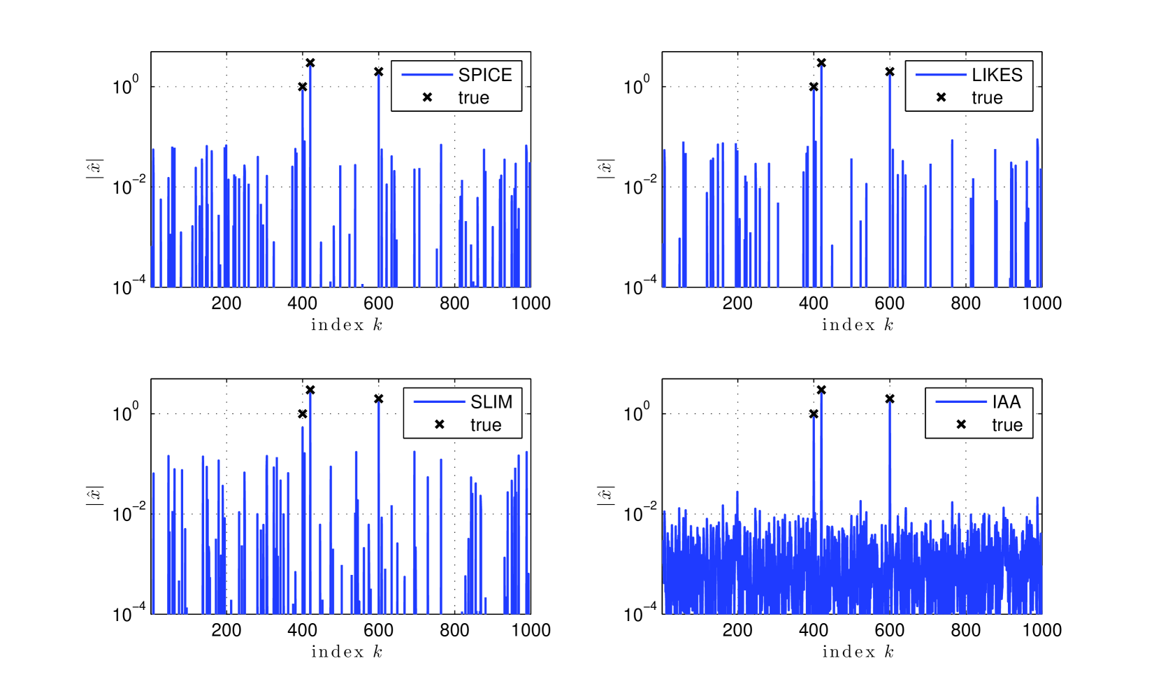
Figure 1 illustrates the ability of the four algorithms to locate the active coefficients $\{x_{k}\}_{k\in S}$ and provide reasonably small estimates of $\{x_{k}\}_{k\not\in S}$, for a randomly selected realization. Likes and Iaa produce sparser respectively denser estimates than Spice. Note that the magnitude of Iaa estimates for $k\not\in S$ is substantially lower than for the other algorithms.

Figure 1: Estimates $|\hat{x}_{k}|$ versus $k$ for a randomly selected realization. $N=35$ samples and $\text{SNR}=20$ dB.

A plausible explanation of this is that the power estimates for $k\not\in S$ capture a fraction of the residual power. Thus a ‘quasi-sparse’ method like Iaa will spread this residual power more evenly across $k\not\in S$, than a sparse method such as Slim which will concentrate it into fewer nonzero estimates.

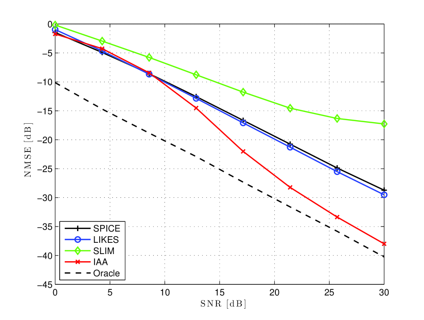
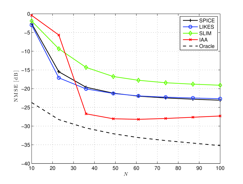
Figures 2 and 3 show the mean square error metric $\text{MSE}\triangleq\operatorname{E}[\|\boldsymbol{x}-\hat{\boldsymbol{x}}\|^{2}_{2}]$, normalized by the signal power $\operatorname{E}[\|\boldsymbol{x}\|^{2}_{2}]$. This metric quantifies the ability of the methods to localize $k\in S$ as well as provide reasonably small estimates for $k\not\in S$. For reference we have added the performance of an ‘oracle’ estimator for which the unknown support set $S$ is given; it computes the LS estimate for these coefficients, the performance of which provides a lower MSE bound. Note that as $M=1000$, the uniqueness condition $M+N<N^{2}$, is satisfied when $N\geq 33$, cf. Section III. Observe that when $N$ is above this threshold, Iaa performs better than the other algorithms in terms of MSE. This MSE reduction is mainly attributable to Iaa’s ability to provide smaller coefficient estimates for $k\not\in S$.

Figure 2: Normalized MSE versus SNR for the IID regression problem, $N=35$ samples.

Figure 3: Normalized MSE versus $N$ for the IID regression problem, $\text{SNR}=20$ dB.

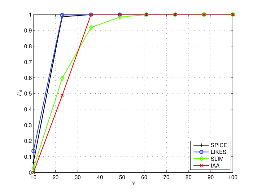
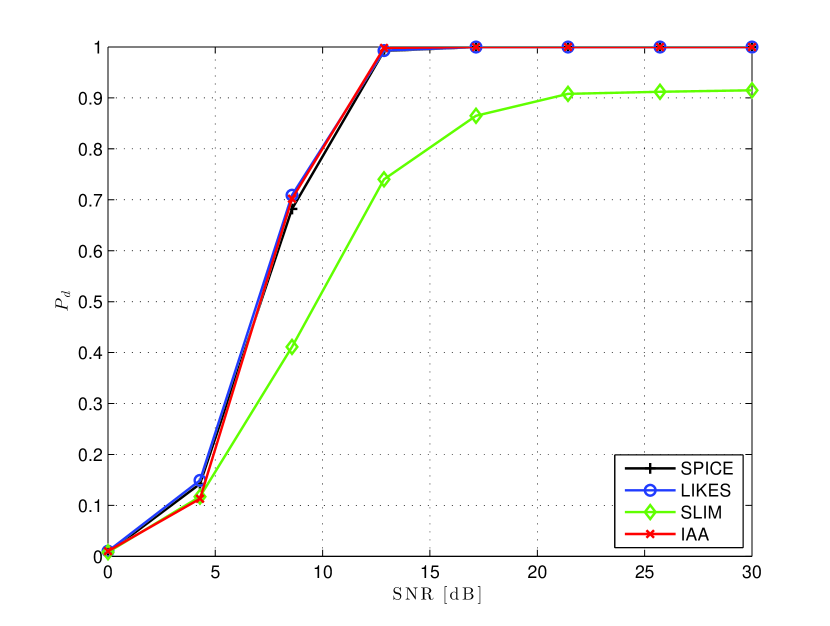
The next two figures show plots of the support-set detection rate, $P_{d}\triangleq\Pr\{S=\hat{S}\}$. We obtain the estimated support set, $\hat{S}$, for each algorithm as the set of indices corresponding to the $K=3$ largest values of $\hat{p}_{k}$, $k=1,\dots,M$. Figures 4 and 5 show $P_{d}$ as a function of SNR and $N$. We can see that $P_{d}$ approaches 1 for all algorithms as $N$ increases, and also that Spice and Likes perform the best in the low sample scenario. The performance of the standard beamformer was too low for visibility and therefore omitted.

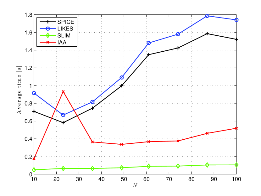
Finally, Figure 6 shows the average computation time until convergence for each algorithm. While the implementations are not carefully optimized, the figure should illustrate at least the relative order of the algorithms. Noticeably, in the IID case with the present signal dimensions, Spice tends to be slower than Slim and Iaa which update their weights adaptively. Not only does the performance of Iaa degrade when $N<33$, but the algorithm tends to require more iterations until convergence.

Figure 4: Probability of correct support-set detection $P_{d}$ versus SNR for the IID regression problem, $N=35$ samples.

Figure 5: Probability of correct support-set detection $P_{d}$ versus $N$ for the IID regression problem, $\text{SNR}=20$ dB.

Figure 6: Average computation time versus $N$ for the IID regression problem, $\text{SNR}=20$ dB.

VI-B Steering-vector regressors

We now consider estimating the directions of arrival of the source signals impinging on a uniform linear array (ULA) with half-wavelength separation between elements. In this problem the locations of the nonzero components of $\boldsymbol{x}$ are of interest rather than $\boldsymbol{x}$ itself. The columns of $\boldsymbol{B}=[\boldsymbol{b}(\theta_{1})\cdots\boldsymbol{b}(\theta_{M})]$ are given by the array steering vector $\boldsymbol{b}(\theta)=[1\>e^{-j\kappa\sin\theta}\>\cdots\>e^{-j(N-1)\kappa\sin\theta}]^{\top}$ [22], and a uniform grid of angles $\{\theta_{k}\}^{M}_{k=1}\subset[-90^{\circ},90]$. We consider $K=3$ sources located at $\theta_{k}$, $k\in S=\{400,420,600\}$ on the grid. This corresponds to DOAs at approximately $-18.1^{\circ}$, $-14.5^{\circ}$ and $17.9^{\circ}$, respectively. As before the amplitudes for $k\in S$ are generated as $x_{k}=|x_{k}|e^{j\phi_{k}}$ with fixed powers $\{1,9,4\}$, respectively, and uniformly drawn phases.

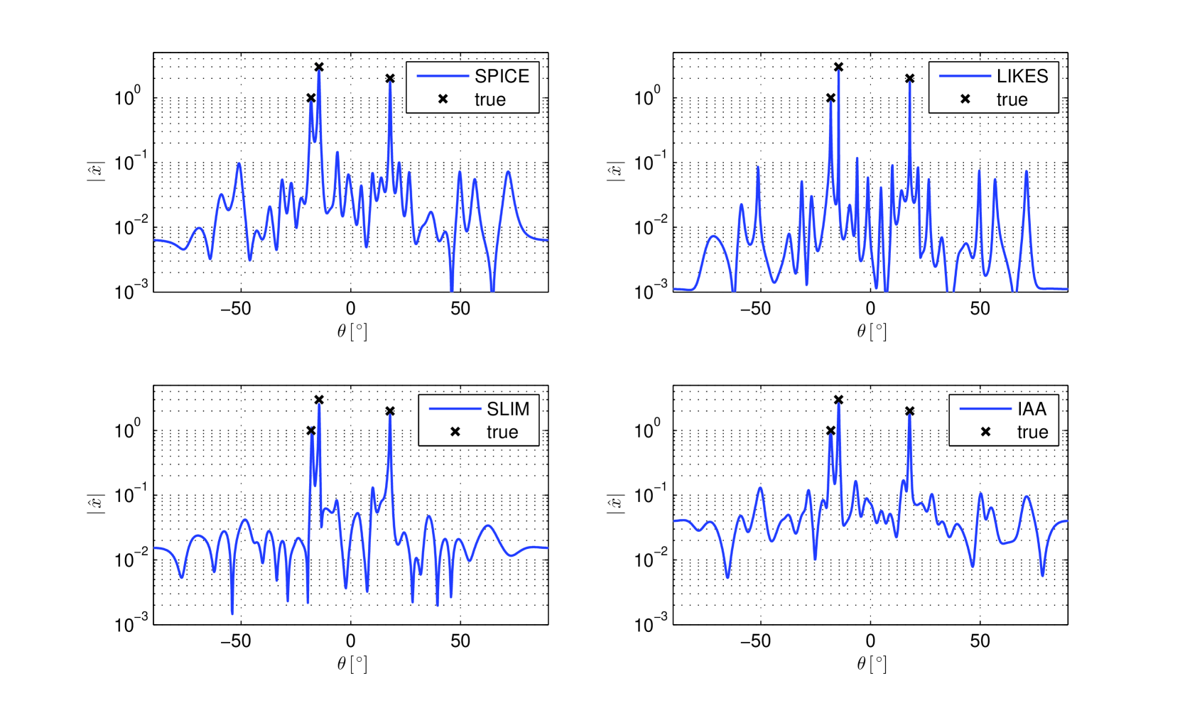
Figure 7 illustrates the ability of the four algorithms to locate the sources and estimate their amplitudes in a randomly selected realization. The estimates $\hat{x}_{k}$ are computed using the Capon formula (4) which in the present case is less biased towards zero than (3). Note that Likes produces sharper spectral estimates than the other algorithms.

Figure 7: Estimates $|\hat{x}_{k}|$ in a randomly selected realization. $N=35$ sensors and $\text{SNR}=20$ dB.

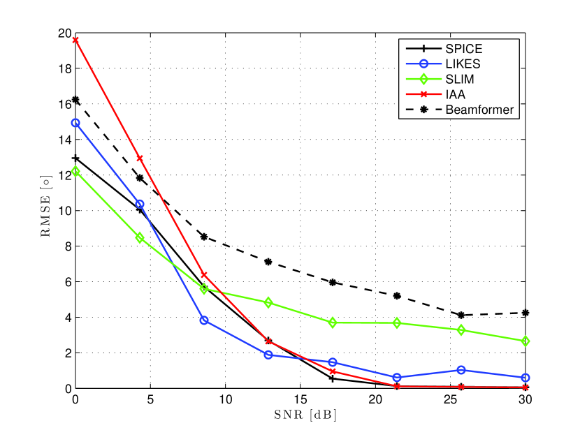
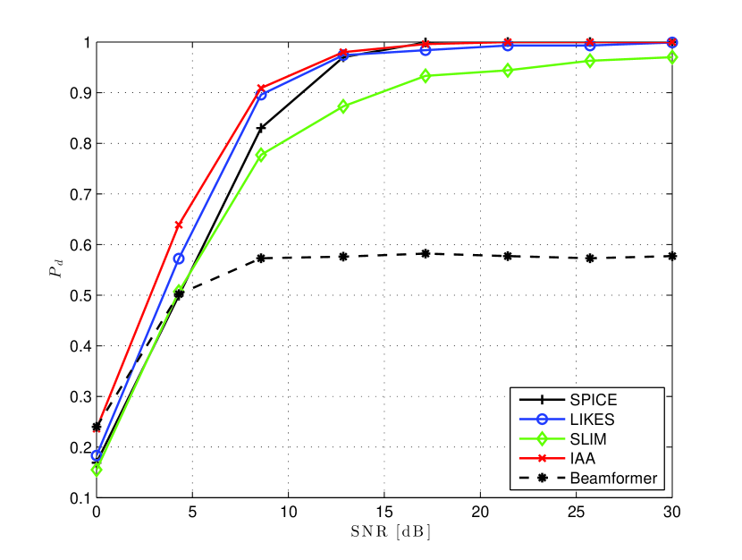
Next, we quantify the accuracy of the DOA estimates $\{\hat{\theta}_{k}\}$ obtained from the locations of the three peaks of $\{\hat{p}_{k}\}^{M}_{k=1}$. In Figure 8 we plot the root MSE per source, $\text{RMSE}\triangleq\sqrt{\frac{1}{K}\operatorname{E}[\|\boldsymbol{\theta}-\hat{\boldsymbol{\theta}}\|^{2}_{2}]}$, where $\boldsymbol{\theta}$ and $\hat{\boldsymbol{\theta}}$ denote the vectors of ordered DOAs and estimates, respectively. For reference, we have also included the standard-beamformer performance. As SNR increases above 10 dB the errors of Spice, Likes and Iaa fall well below the RMSE of the beamformer. Figure 9 shows the probability of detecting the $K$ sources within $\Delta\theta$ degrees from the true DOA, $P_{d}\triangleq\Pr\{|\theta_{i}-\hat{\theta}_{i}|<\Delta\theta,\forall i\}$. Here we set $\Delta\theta$ to half of the distance between the two closely-spaced DOAs, i.e., $\Delta\theta=1.8^{\circ}$. For this metric, Iaa turns out to perform at least slightly better than the other algorithms which all locate the peaks substantially better than the beamformer. For a further analysis of the resolution limit of sparse methods, see [36, 37].

Figure 8: Root mean square error of DOA estimates, per source, versus SNR. $N=35$ sensors.

Figure 9: Probability of detection $P_{d}$ versus SNR for steering-vector regressors, $N=35$ sensors.

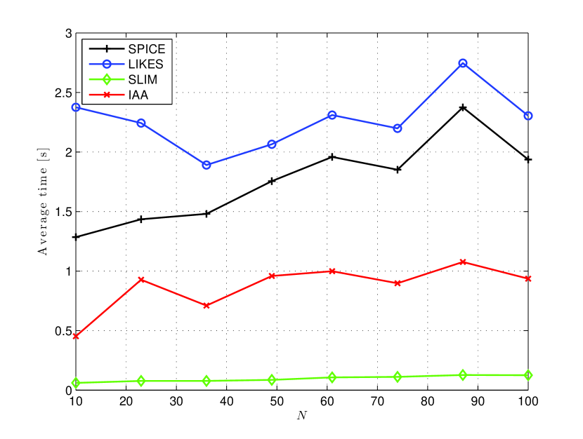
Figure 10 illustrates the average computation time versus $N$, and the order of the algorithms is the same as in Figure 6. Recall that Slim is set to terminate after 5 iterations.

Figure 10: Average computation time versus $N$ for steering-vector regressors, $\text{SNR}=20$ dB.

VII Conclusions

In this article we have presented a framework for sparse parameter estimation based on the Spice fitting criterion and a gradient optimization approach. This framework was shown to have several appealing features:

• It unifies four hyperparameter-free methods, namely Spice, Likes, Slim and Iaa, the latter three methods being instances of Spice with adaptive weights.

• It enables further insights into the above four algorithms, including the analysis of their convergence properties and statistical performance. In particular, we showed how the weights used by these methods determine the sparsity of their corresponding estimates.

• Finally, it makes it possible to derive new versions of the algorithms by considering different step-lengths in the gradient approach.

We also investigated the covariance model upon which the Spice criterion is based, and:

• Provided identifiability conditions for this model.

• Showed that depending on whether the noise powers are modeled nonuniformly or uniformly, the Spice method coincides with the $\ell_{1}$-penalized Lad or the square-root Lasso problems. This fact also established a connection between the latter two methods.

The four hyperparameter-free methods were evaluated in two different inference problems with IID and steering-vector regressors, respectively. The results indicated that:

• The a-version algorithms appear to be better than the b-versions in terms of convergence and statistical performance.

• In problems with IID regressors both Spice and Likes perform similarly and they exhibit a graceful degradation as the number of samples decreases. For a sufficient number of samples, such that $M+N<N^{2}$, the ‘quasi-sparse’ Iaa method, however, was found to provide smaller parameter estimates for the true zero coefficients.

• In the steering-vector regressor case the peaks of the amplitude spectrum using the Capon formula were less biased towards zero than when using the LMMSE formula. Likes was computationally more demanding than the rest, but produced a sparser amplitude spectrum. For locating spectral peaks, however, Iaa was found to perform slightly better than the rest.

Appendix A The multisnapshot case

The Spice criterion (7) extends to the multisnapshot scenario as follows:

$$\begin{split}\|\boldsymbol{R}^{-1/2}(\bar{\boldsymbol{R}}-\boldsymbol{R})\|^{2}_{F}&=\text{tr}\{(\bar{\boldsymbol{R}}-\boldsymbol{R})\boldsymbol{R}^{-1}(\bar{\boldsymbol{R}}-\boldsymbol{R})\}\\ &=\text{tr}\{\bar{\boldsymbol{R}}\boldsymbol{R}^{-1}\bar{\boldsymbol{R}}\}+\text{tr}\{\boldsymbol{R}\}+\text{const.},\end{split}$$ (43)

where $\bar{\boldsymbol{R}}\triangleq\frac{1}{T}\sum^{T}_{t=1}\boldsymbol{y}_{t}\boldsymbol{y}^{*}_{t}$ and $T$ is the number of snapshots (possibly $T<N$). The derivative of (43) w.r.t. $p_{k}$ is equal to

$$-\text{tr}\left\{\bar{\boldsymbol{R}}\boldsymbol{R}^{-1}\frac{\partial\boldsymbol{R}}{\partial p_{k}}\boldsymbol{R}^{-1}\bar{\boldsymbol{R}}\right\}+w_{k}=-\|\boldsymbol{a}^{*}_{k}\boldsymbol{R}^{-1}\bar{\boldsymbol{R}}\|^{2}_{2}+w_{k}.$$

Then the Spice algorithms (24) and (26) become

$$\hat{p}^{i+1}_{k}=\hat{p}^{i}_{k}\|\boldsymbol{a}^{*}_{k}\widehat{\boldsymbol{R}}^{-1}_{i}\bar{\boldsymbol{R}}\|_{2}/w^{1/2}_{k}\quad(\text{{Spice}}_{\text{a}})$$ (44)

and, respectively,

$$\hat{p}^{i+1}_{k}=\hat{p}^{i}_{k}\|\boldsymbol{a}^{*}_{k}\hat{\boldsymbol{R}}^{-1}_{i}\bar{\boldsymbol{R}}\|^{2}_{2}/w_{k}\quad(\text{{Spice}}_{\text{b}}).$$ (45)

When the number of snapshots $T\geq N$ one may use a modified cost function, viz. $\|\boldsymbol{R}^{-1/2}(\bar{\boldsymbol{R}}-\boldsymbol{R})\bar{\boldsymbol{R}}^{-1/2}\|^{2}_{F}$, cf. [15].

Appendix B Lemma proofs

Lemma 1

The inquality in (6) follows if we can show that $\widehat{\boldsymbol{P}}^{-1}\succeq\boldsymbol{A}^{*}\widehat{\boldsymbol{R}}^{-1}\boldsymbol{A}$ or, equivalently, $\boldsymbol{I}_{M}-\widehat{\boldsymbol{P}}^{1/2}\boldsymbol{A}^{*}(\boldsymbol{A}\widehat{\boldsymbol{P}}\boldsymbol{A}^{*})^{-1}\boldsymbol{A}\widehat{\boldsymbol{P}}^{1/2}\succeq\boldsymbol{0}$; however this is obviously true since the left hand side is the orthogonal projection matrix onto the null space of $\boldsymbol{A}\widehat{\boldsymbol{P}}^{1/2}$.

Lemma 2

We have that

$$\begin{split}cf(\bar{\boldsymbol{p}})\bigr{|}_{\bar{\boldsymbol{p}}=c\boldsymbol{p}}&=c\boldsymbol{y}^{*}(\boldsymbol{A}c\boldsymbol{P}\boldsymbol{A}^{*})^{-1}\boldsymbol{y}+c\sum^{M+N}_{k=1}w_{k}cp_{k}\\ &=\boldsymbol{y}^{*}\boldsymbol{R}^{-1}\boldsymbol{y}+c^{2}\sum^{M+N}_{k=1}w_{k}p_{k}\\ &=g(\boldsymbol{p})\end{split}$$

and thus

$$cf(c\hat{\boldsymbol{p}})=g(\hat{\boldsymbol{p}})\leq g(\boldsymbol{p})=cf(c\boldsymbol{p}),\>\forall\{p_{k}\geq 0\}$$

which implies:

$$f(\hat{\bar{\boldsymbol{p}}})\leq f({\bar{\boldsymbol{p}}}),\forall\{\bar{p}_{k}\geq 0\},$$

and this concludes the proof.

Lemma 3

A simple calculation yields:

$$\begin{split}&(\boldsymbol{y}-\boldsymbol{B}\boldsymbol{x})^{*}\boldsymbol{S}^{-1}(\boldsymbol{y}-\boldsymbol{B}\boldsymbol{x})\\ &=\boldsymbol{y}^{*}\boldsymbol{S}^{-1}\boldsymbol{y}-\boldsymbol{y}^{*}\boldsymbol{S}^{-1}\boldsymbol{B}\boldsymbol{x}-\boldsymbol{x}^{*}\boldsymbol{B}^{*}\boldsymbol{S}^{-1}\boldsymbol{y}+\boldsymbol{x}^{*}\boldsymbol{B}^{*}\boldsymbol{S}^{-1}\boldsymbol{B}\boldsymbol{x}\end{split}$$

Therefore the criterion in (11) can be re-written as:

$$\boldsymbol{x}^{*}(\boldsymbol{B}^{*}\boldsymbol{S}^{-1}\boldsymbol{B}+\boldsymbol{\Pi}^{-1})\boldsymbol{x}-\boldsymbol{x}^{*}\boldsymbol{B}^{*}\boldsymbol{S}^{-1}\boldsymbol{y}-\boldsymbol{y}^{*}\boldsymbol{S}^{-1}\boldsymbol{B}\boldsymbol{x}+\text{constant},$$

which yields the minimizer

$$\hat{\boldsymbol{x}}=(\boldsymbol{B}^{*}\boldsymbol{S}^{-1}\boldsymbol{B}+\boldsymbol{\Pi}^{-1})^{-1}\boldsymbol{B}^{*}\boldsymbol{S}^{-1}\boldsymbol{y}.$$ (46)

Next, note that

$$\begin{split}(\boldsymbol{B}^{*}\boldsymbol{S}^{-1}\boldsymbol{B}+\boldsymbol{\Pi}^{-1})\boldsymbol{\Pi}\boldsymbol{B}^{*}&=\boldsymbol{B}^{*}\boldsymbol{S}^{-1}\boldsymbol{B}\boldsymbol{\Pi}\boldsymbol{B}^{*}+\boldsymbol{B}^{*}\\ &=\boldsymbol{B}^{*}\boldsymbol{S}^{-1}(\boldsymbol{B}\boldsymbol{\Pi}\boldsymbol{B}^{*}+\boldsymbol{S})\end{split}$$

or equivalently,

$$(\boldsymbol{B}^{*}\boldsymbol{S}^{-1}\boldsymbol{B}+\boldsymbol{\Pi}^{-1})^{-1}\boldsymbol{B}^{*}\boldsymbol{S}^{-1}=\boldsymbol{\Pi}\boldsymbol{B}^{*}(\boldsymbol{B}\boldsymbol{\Pi}\boldsymbol{B}^{*}+\boldsymbol{S})^{-1},$$

which means that (46) can be re-written as in (12).

It remains to evaluate the criterion at $\hat{\boldsymbol{x}}$. Because

$$\begin{split}\boldsymbol{y}-\boldsymbol{B}\hat{\boldsymbol{x}}&=(\boldsymbol{I}_{M}-\boldsymbol{B}\boldsymbol{\Pi}\boldsymbol{B}^{*}\boldsymbol{R}^{-1})\boldsymbol{y}\\ &=(\boldsymbol{R}-\boldsymbol{B}\boldsymbol{\Pi}\boldsymbol{B}^{*})\boldsymbol{R}^{-1}\boldsymbol{y}\\ &=\boldsymbol{S}\boldsymbol{R}^{-1}\boldsymbol{y}\end{split}$$

we have

$$\begin{split}&(\boldsymbol{y}-\boldsymbol{B}\hat{\boldsymbol{x}})^{*}\boldsymbol{S}^{-1}(\boldsymbol{y}-\boldsymbol{B}\hat{\boldsymbol{x}})+\hat{\boldsymbol{x}}^{*}\boldsymbol{\Pi}^{-1}\hat{\boldsymbol{x}}\\ &=\boldsymbol{y}^{*}\boldsymbol{R}^{-1}\boldsymbol{S}\boldsymbol{R}^{-1}\boldsymbol{y}+\boldsymbol{y}^{*}\boldsymbol{R}^{-1}\boldsymbol{B}\boldsymbol{\Pi}\boldsymbol{B}^{*}\boldsymbol{R}^{-1}\boldsymbol{y}\\ &=\boldsymbol{y}^{*}\boldsymbol{R}^{-1}\boldsymbol{y}\end{split}$$

which concludes the proof.

Appendix C Spice for identical noise powers

In this case the covariance model becomes:

$$\boldsymbol{R}=\boldsymbol{B}\boldsymbol{\Pi}\boldsymbol{B}^{*}+\sigma^{2}\boldsymbol{I}_{N}$$ (47)

and (11) becomes

$$\min_{\boldsymbol{x}}\|\boldsymbol{y}-\boldsymbol{B}\boldsymbol{x}\|^{2}_{2}/\sigma^{2}+\sum^{M}_{k=1}|x_{k}|^{2}/p_{k}=\boldsymbol{y}^{*}\boldsymbol{R}^{-1}\boldsymbol{y}.$$

It follows that the minimizers $\{p_{k}\}$ of the Spice criterion can also be obtained by minimizing the function:

$$\|\boldsymbol{y}-\boldsymbol{B}\boldsymbol{x}\|^{2}_{2}/\sigma^{2}+\sum^{M}_{k=1}|x_{k}|^{2}/p_{k}+\sum^{M}_{k=1}w_{k}p_{k}+\underbrace{\left(\sum^{M+N}_{k=M+1}w_{k}\right)}_{w^{2}}\sigma^{2}.$$ (48)

Minimization of (48) w.r.t. $\sigma^{2}$ and $\{p_{k}\}$ gives:

$$\begin{split}\sigma^{2}&=\|\boldsymbol{y}-\boldsymbol{B}\boldsymbol{x}\|_{2}/w\\ p_{k}&=|x_{k}|/\sqrt{w_{k}},\;k=1,\dots,M.\end{split}$$ (49)

Inserting (49) in (48) yields (to within a multiplicative factor):

$$w\|\boldsymbol{y}-\boldsymbol{B}\boldsymbol{x}\|_{2}+\|\text{diag}(\sqrt{w_{1}},\dots,\sqrt{w_{M}})\boldsymbol{x}\|_{1}$$

which is the criterion of the square-root Lasso (with weights for the $\ell_{1}$-norm of $\boldsymbol{x}$). The above proof is more direct than the one in [26, 27].

Appendix D Cyclic minimization interpretation

The gradient approach in Section IV is simple and quite flexible; unlike the cyclic minimization approach in [14, 15, 16], the gradient approach produced not only the original algorithms but also different versions of them. However, the gradient approach cannot be used to conclude the monotonic decrease property used in the convergence analysis in Section V. Indeed, while the function

$$f(\boldsymbol{p})=\boldsymbol{y}^{*}\boldsymbol{R}^{-1}\boldsymbol{y}+\sum^{M+N}_{k=1}w_{k}p_{k}\quad(w_{k}\text{ given})$$

is convex, the gradient-based algorithms might overshoot the minimum, and hence they are not guaranteed to monotonically decrease this function. To prove such a property we need the cyclic minimization framework.

Let

$$g(\boldsymbol{\beta},\boldsymbol{p})=\sum^{M+N}_{k=1}\left(\frac{|\beta_{k}|^{2}}{p_{k}}+w_{k}p_{k}\right)$$ (50)

(the augmented function used by this framework). As shown in [14, 15, 16]

$$\min_{\boldsymbol{\beta}}g(\boldsymbol{\beta},\boldsymbol{p})=\boldsymbol{y}^{*}\boldsymbol{R}^{-1}\boldsymbol{y}+\sum^{M+N}_{k=1}w_{k}p_{k}\quad(\text{s.t. }\boldsymbol{A}\boldsymbol{\beta}=\boldsymbol{y})$$ (51)

and the minimum is attained at

$$\hat{\beta}_{k}=p_{k}\boldsymbol{a}^{*}_{k}\boldsymbol{R}^{-1}\boldsymbol{y}.$$ (52)

To show this result, let

$$\boldsymbol{\beta}=\begin{bmatrix}\boldsymbol{x}\\ \boldsymbol{y}-\boldsymbol{B}\boldsymbol{x}\end{bmatrix}$$

which satisfies the constraint in (51); then clearly the result is equivalent to Lemma 3.

It follows from (51) that to get $\boldsymbol{p}$ that minimizes $f(\boldsymbol{p})$ we can cyclically minimize $g(\boldsymbol{\beta},\boldsymbol{p})$ w.r.t. $\boldsymbol{\beta}$ and $\boldsymbol{p}$. For given $\boldsymbol{p}$, the minimizing $\boldsymbol{\beta}$ is given by (52). For a given $\boldsymbol{\beta}$, the minimization of $g(\boldsymbol{\beta},\boldsymbol{p})$ w.r.t. $\boldsymbol{p}$ yields

$$\hat{\boldsymbol{p}}_{k}=|\beta_{k}|/w^{1/2}_{k}.$$ (53)

Iteratively, this means (combining (52) and (53) into one equation):

$$\hat{p}^{i+1}_{k}=\hat{p}^{i}_{k}|\boldsymbol{a}^{*}_{k}\boldsymbol{R}^{-1}_{i}\boldsymbol{y}|/w^{1/2}_{k}$$ (54)

which is (24). Therefore, for (24) the monotonic decreasing property of $f(\boldsymbol{p})$ is guaranteed:

$$f(\hat{\boldsymbol{p}}^{i})=g(\hat{\boldsymbol{\beta}}^{i},\hat{\boldsymbol{p}}^{i})\geq g(\hat{\boldsymbol{\beta}}^{i},\hat{\boldsymbol{p}}^{i+1})\geq g(\hat{\boldsymbol{\beta}}^{i+1},\hat{\boldsymbol{p}}^{i+1})\geq f(\hat{\boldsymbol{p}}^{i+1}).$$ (55)

But does this property hold for (26) as well? For (26), i.e.,

$$\hat{p}^{i+1}_{k}=\hat{p}^{i}_{k}|\boldsymbol{a}^{*}_{k}\boldsymbol{R}^{-1}_{i}\boldsymbol{y}|^{2}/w_{k}$$

we have that:

$$\begin{split}\frac{|\hat{\beta}^{i}_{k}|^{2}}{\hat{p}^{i+1}_{k}}+w_{k}\hat{p}^{i+1}_{k}&=\frac{(\hat{p}^{i}_{k})^{2}|\boldsymbol{a}^{*}_{k}\widehat{\boldsymbol{R}}^{-1}_{i}\boldsymbol{y}|^{2}}{\hat{p}^{i}_{k}|\boldsymbol{a}^{*}_{k}\widehat{\boldsymbol{R}}^{-1}_{i}\boldsymbol{y}|^{2}}w_{k}+w_{k}\frac{\hat{p}^{i}_{k}|\boldsymbol{a}^{*}_{k}\widehat{\boldsymbol{R}}^{-1}_{i}\boldsymbol{y}|^{2}}{w_{k}}\\ &=w_{k}\hat{p}^{i}_{k}+\frac{|\hat{\beta}^{i}_{k}|}{\hat{p}^{i}_{k}}.\end{split}$$

Hence

$$g(\hat{\boldsymbol{\beta}}^{i},\hat{\boldsymbol{p}}^{i})=g(\hat{\boldsymbol{\beta}}^{i},\hat{\boldsymbol{p}}^{i+1})$$

and the monotonic decrease property holds for (26) too (owing to the second inequality in (55)).

References

• [1] T. Hastie, R. Tibshirani, and J. Friedman, The Elements of Statistical Learning: Data Mining, Inference, and Prediction, Second Edition. Springer series in statistics, Springer, 2009.
• [2] E. Candes and M. Wakin, “An introduction to compressive sampling,” IEEE Signal Processing Magazine, vol. 25, no. 2, pp. 21–30, 2008.
• [3] M. Elad, Sparse and Redundant Representations: From Theory to Applications in Signal and Image Processing. Springer, 2010.
• [4] D. Malioutov, M. Cetin, and A. Willsky, “A sparse signal reconstruction perspective for source localization with sensor arrays,” IEEE Trans. Signal Processing, vol. 53, no. 8, pp. 3010–3022, 2005.
• [5] S. Bourguignon, H. Carfantan, and J. Idier, “A sparsity-based method for the estimation of spectral lines from irregularly sampled data,” IEEE J. Selected Topics in Signal Processing, vol. 1, no. 4, pp. 575–585, 2007.
• [6] M. Lustig, D. Donoho, J. Santos, and J. Pauly, “Compressed sensing MRI,” IEEE Signal Processing Magazine, vol. 25, no. 2, pp. 72–82, 2008.
• [7] R. Tibshirani, “Regression shrinkage and selection via the lasso,” J. Royal Statistical Society. Series B (Methodological), vol. 58, no. 1, pp. 267–288, 1996.
• [8] V. Roth, “The generalized LASSO,” IEEE Trans. Neural Networks, vol. 15, no. 1, pp. 16–28, 2004.
• [9] S. Chen, D. Donoho, and M. Saunders, “Atomic decomposition by basis pursuit,” SIAM Review, vol. 43, no. 1, pp. 129–159, 2001.
• [10] J. Tropp, “Just relax: convex programming methods for identifying sparse signals in noise,” IEEE Trans. Information Theory, vol. 52, no. 3, pp. 1030–1051, 2006.
• [11] J.-J. Fuchs, “On sparse representations in arbitrary redundant bases,” IEEE Trans. Information Theory, vol. 50, no. 6, pp. 1341–1344, 2004.
• [12] B. Efron, T. Hastie, I. Johnstone, and R. Tibshirani, “Least angle regression,” Annals of Statistics, vol. 32, no. 2, pp. 407–499, 2004.
• [13] A. Maleki and D. Donoho, “Optimally tuned iterative reconstruction algorithms for compressed sensing,” IEEE J. Selected Topics in Signal Processing, vol. 4, no. 2, pp. 330–341, 2010.
• [14] P. Stoica, P. Babu, and J. Li, “New method of sparse parameter estimation in separable models and its use for spectral analysis of irregularly sampled data,” IEEE Trans. Signal Processing, vol. 59, no. 1, pp. 35–47, 2011.
• [15] P. Stoica, P. Babu, and J. Li, “SPICE: A sparse covariance-based estimation method for array processing,” IEEE Trans. Signal Processing, vol. 59, no. 2, pp. 629–638, 2011.
• [16] P. Stoica and P. Babu, “SPICE and LIKES: Two hyperparameter-free methods for sparse-parameter estimation,” Signal Processing, vol. 92, no. 7, pp. 1580–1590, 2012.
• [17] X. Tan, W. Roberts, J. Li, and P. Stoica, “Sparse learning via iterative minimization with application to MIMO radar imaging,” IEEE Trans. Signal Processing, vol. 59, no. 3, pp. 1088–1101, 2011.
• [18] T. Yardibi, J. Li, P. Stoica, M. Xue, and A. Baggeroer, “Source localization and sensing: A nonparametric iterative adaptive approach based on weighted least squares,” IEEE Trans. Aerospace and Electronic Systems, vol. 46, no. 1, pp. 425–443, 2010.
• [19] L. Wang, “The penalized LAD estimator for high dimensional linear regression,” J. Multivariate Analysis, vol. 120, pp. 135–151, 2013.
• [20] A. Belloni, V. Chernozhukov, and L. Wang, “Square-root LASSO: pivotal recovery of sparse signals via conic programming,” Biometrika, vol. 98, no. 4, pp. 791–806, 2011.
• [21] S. Kay, Fundamentals of Statistical Signal Processing: Estimation Theory. No. v. 1, Prentice-Hall PTR, 1998.
• [22] P. Stoica and R. Moses, Spectral Analysis of Signals. Prentice Hall, 2005.
• [23] S. Boyd and L. Vandenberghe, Convex Optimization. Cambridge University Press, 2004.
• [24] I. Gorodnitsky and B. Rao, “Sparse signal reconstruction from limited data using FOCUSS: a re-weighted minimum norm algorithm,” IEEE Trans. Signal Processing, vol. 45, no. 3, pp. 600–616, 1997.
• [25] M. Tipping, “Sparse Bayesian learning and the relevance vector machine,” Journal of Machine Learning Research, vol. 1, pp. 211–244, 2001.
• [26] P. Babu and P. Stoica, “Connection between SPICE and square-root LASSO for sparse parameter estimation,” Signal Processing, vol. 95, pp. 10–14, 2014.
• [27] C. Rojas, D. Katselis, and H. Hjalmarsson, “A note on the SPICE method,” IEEE Trans. Signal Processing, vol. 61, no. 18, pp. 4545–4551, 2013.
• [28] N. Sidiropoulos, R. Bro, and G. Giannakis, “Parallel factor analysis in sensor array processing,” IEEE Trans. Signal Processing, vol. 48, no. 8, pp. 2377–2388, 2000.
• [29] T. Jiang, N. Sidiropoulos, and J. ten Berge, “Almost-sure identifiability of multidimensional harmonic retrieval,” IEEE Trans. Signal Processing, vol. 49, no. 9, pp. 1849–1859, 2001.
• [30] B. Ottersten, P. Stoica, and R. Roy, “Covariance matching estimation techniques for array signal processing applications,” Digital Signal Processing, vol. 8, no. 3, pp. 185–210, 1998.
• [31] E. Candès, M. Wakin, and S. Boyd, “Enhancing sparsity by reweighted l1 minimization,” J. Fourier Analysis and Applications, vol. 14, no. 5-6, pp. 877–905, 2008.
• [32] P. Stoica and Y. Selen, “Cyclic minimizers, majorization techniques, and the expectation-maximization algorithm: a refresher,” IEEE Signal Processing Magazine, vol. 21, no. 1, pp. 112–114, 2004.
• [33] W. I. Zangwill, Nonlinear Programming: a Unified Approach. Prentice-Hall Englewood Cliffs, NJ, 1969.
• [34] W. Roberts, P. Stoica, J. Li, T. Yardibi, and F. Sadjadi, “Iterative adaptive approaches to MIMO radar imaging,” IEEE J. Selected Topics in Signal Processing, vol. 4, no. 1, pp. 5–20, 2010.
• [35] C. Kelley, Iterative Methods for Linear and Nonlinear Equations. Frontiers in Applied Mathematics, Society for Industrial and Applied Mathematics, 1995.
• [36] E. J. Candès, J. Romberg, and T. Tao, “Robust uncertainty principles: Exact signal reconstruction from highly incomplete frequency information,” IEEE Trans. Information Theory, vol. 52, no. 2, pp. 489–509, 2006.
• [37] S. Fortunati, R. Grasso, G. R., and M. Greco, “Single snapshot DOA estimation using compressed sensing,” in Proc. IEEE Int. Conf. Acoustics, Speech and Signal Processing (ICASSP), pp. 2316–2320, May 2014.