Cooee bitumen II: Stability of linear asphaltene nanoaggregates

Abstract

Asphaltene and smaller aromatic molecules tend to form linear nanoaggregates in bitumen. Over the years bitumen undergoes chemical aging and during this process, the size of the nanoaggregate increases. This increase is associated with an increase in viscosity and brittleness of the bitumen, eventually leading to road deterioration. This paper focuses on understanding the mechanisms behind nanoaggregate size and stability. We used molecular dynamics simulations to quantify the probability of having a nanoaggregate of a given size in the stationary regime. To model this complicated behavior, we chose first to consider the simple case where only asphaltene molecules are counted in a nanoaggregate. We used a master equation approach and a related statistical mechanics model. The linear asphaltene nanoaggregates behave as a rigid linear chain. The most complicated case where all aromatic molecules are counted in a nanoaggregate is then discussed. The linear aggregates where all aromatic molecules are counted seem to behave as a flexible linear chain.

Corresponding author: C. A. Lemarchand, E-mail: clairel@ruc.dk

I Introduction

One of the main industrial applications of bitumen is as a binder in asphalt pavement [ec140, ]. Bitumen links together mineral aggregates and filler particles to form a cohesive asphalt on the road surface. Over the years, a chemical reaction takes place in bitumen increasing the number of heavy aromatic molecules [ec140, ; shrp368, ; herrington, ; lu, ; petersen74, ]. This process is called chemical aging. The aromatic molecules in bitumen, especially the asphaltene molecules, tend to align to form nanoaggregates. The aging reaction leads also to an increase in the nanoaggregate size [ec140, ; mullins2012, ; aging, ] correlated with an unwanted increase in bitumen viscosity and brittleness [shrp368, ; herrington, ; lu, ; ec140, ; petersen74, ]. The change in bitumen mechanical properties, which go from ”liquid-like” to more ”solid-like” during chemical aging finally results in cracks in the pavement and road deterioration. To prevent or reverse the effects of chemical aging, a first step is to gather more knowledge about the nanoaggregate structure and stability in bitumen.

Much progress has been made over the last 50 years in the experimental and numerical literature to determine the structure of the nanoaggregates and the conditions under which they are formed. One can cite in particular the design of the Yen-Mullins model [yen, , mullins2012, ] describing the nanoaggregate structure, the determination of the critical nanoaggregate concentration in different solvents [andreatta, , goual, ], the evaluation of the average size and polydispersity of a nanoaggregate [eyssautier2011, ] on the experimental side. On the numerical side, different stable conformations of nanoaggregates were identified depending on the asphaltene structure using molecular mechanical calculations [murgich1996, ] and molecular dynamics (MD) simulations [pacheco2004, ]. MD simulations were also used to determine the molecular orientation inside the nanoaggregates [zhang2007, ], and the effects of solvent and presence of other molecules on the nanoaggregate structure [headen2011, ]. However, analytical models for the thermodynamics stability and dynamics of the nanoaggregates in relation to their structure are still quite rare, to the notable exception of Ref. [aguilera2006, ]. The purpose of this paper is precisely to suggest simple and generic models, which can reproduce MD results on the nanoaggregate stability.

We present molecular dynamics results concerning the nanoaggregate size in the stationary regime. In bitumen, nanoaggregates are composed of asphaltene molecules, the most heavy and aromatic fraction in bitumen, but also of lighter aromatic molecules like resin and resinous oil [aging, ]. We give results on the probability of having a nanoaggregate containing a given number of aromatic molecules and the probability of having a nanoaggregate containing a given number of asphaltene molecules. The two probabilities are shown to differ qualitatively. We first model the simpler case, where only asphaltene molecules are counted. The focus in this case is to establish a mechanism for the nanoaggregation of asphaltene molecules. From this aggregation mechanism, a master equation and a statistical mechanics model are derived and provide a simple theoretical framework for interpreting the simulation results on nanoaggregate stability. The results of the master equation approach are also compared to the aggregation dynamics observed in the MD simulations. Then, the more complicated case where all aromatic molecules are counted is discussed in terms of statistical mechanics arguments.

The MD simulations carried out in this work are based on the four-component united-atom-unit model developed in Ref. [us, ] in the framework of the COOEE project [cooee, ]. The model is shown to reproduce a generic bitumen reasonably well [us, ]. The simulations were performed on Graphic-Processor-Units (GPU) using the Roskilde University Molecular Dynamics (RUMD.org) package [rumd, ].

The paper is organized as follows. In Sec. II, we provide simulation details, give a definition of a linear nanoaggregate, and present the MD results about the probability of having a nanoaggregate of a given size. Section III is devoted to model the results on the stability of linear aggregates where only asphaltene molecules are counted with a master equation approach. In Sec. IV, a related statistical mechanics model is described and shown to reproduce the MD results on asphaltene nanoaggregate stability. The more complicated case where all aromatic molecules are counted in a nanoaggregate is also discussed in Sec. IV in terms of statistical mechanics arguments. Sec. V includes a comparison of our results to existing experimental and numerical results and discuss the limit of our model. Finally, Sec. VI contains a summary and a conclusion.

II Molecular dynamics results

Before presenting the molecular dynamics (MD) results on nanoaggregate stability, we mention a few details about the simulations and define precisely a nanoaggregate.

II.1 Simulation details

As mentioned in the introduction, the simulation method and molecular potentials are described in details in Ref. [us, ]. Only information necessary to understand the study on nanoaggregate stability carried out in the present paper is given here.

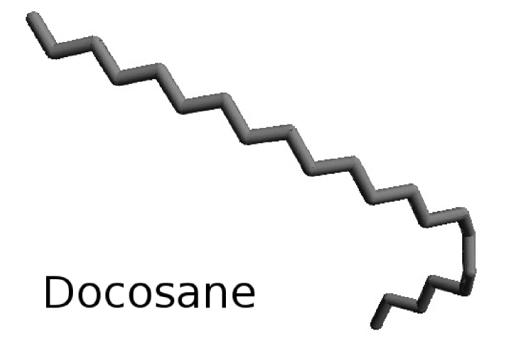
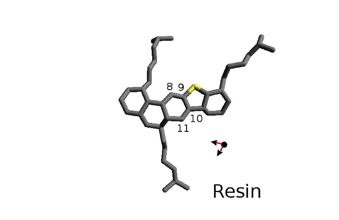
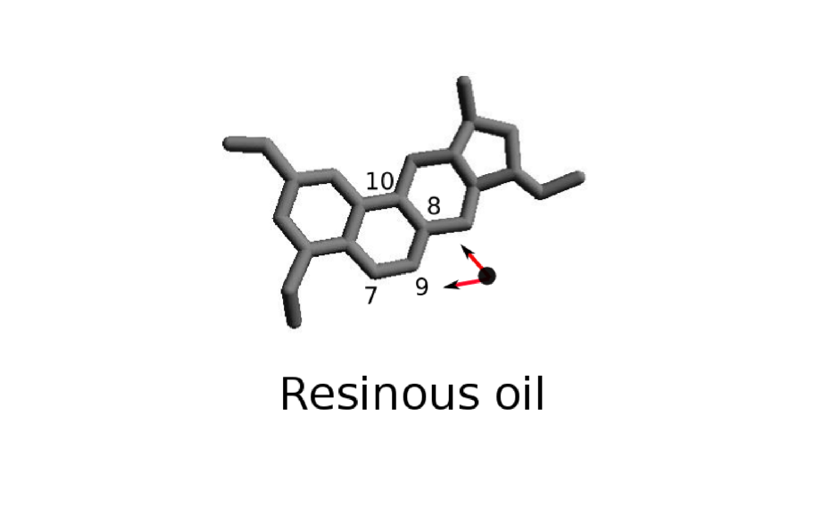
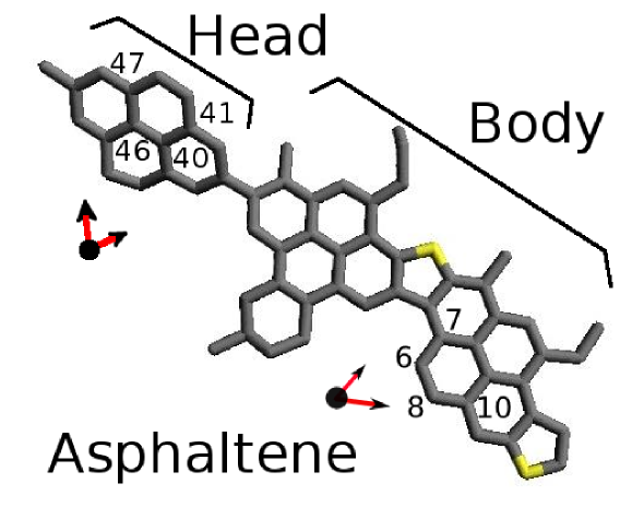
The simulated system contains four types of molecule, chosen to resemble the SARA classification [SARA, ]: a Saturated hydrocarbon, a resinous oil molecule, which is denoted Aromatic in the SARA scheme, a Resin molecule and an Asphaltene molecule. The molecular structures chosen are shown in Fig. 1. The main system studied in this paper contains $410$ saturated hydrocarbons, $50$ resinous oil molecules, $50$ resin molecules and $50$ asphaltene molecules, which corresponds to $15570$ united atom units. The methyl (CH₃), methylene (CH₂), and methine (CH) groups are represented by the same united atom unit of molar mass 13.3 g$\cdot$mol^-1 and the sulfur atoms are represented by a united atom unit with a different molar mass 32 g$\cdot$mol^-1. The potential between the united atom units contains four terms: an intermolecular potential, corresponding to a Lennard-Jones potential with parameters $\sigma=3.75$ Å and $\epsilon/k_{B}=75.4$ K, where $k_{B}$ is the Boltzmann constant and three terms for the intramolecular potential. These three terms describe the bond length between two connected particles, the angle between three consecutive particles, and the dihedral angle between four consecutive particles. The parametrization of the intramolecular potential is described in details in Refs [us, ]. The simulations are performed in the canonical ensemble (NVT) at a constant temperature $T=452$ K and a constant density. The density $\rho=0.964$ kg$\cdot$L^-1 is chosen to obtain an average pressure around the atmospheric pressure. A Nosé-Hoover thermostat is used. The time step is $\Delta t=0.86$ fs and the duration of the simulations is $T=360$ ns. Eight independent simulations are performed at the same state point. The molecular dynamics package RUMD [rumd, ] is used to perform the calculation.

Figure 1: (Color online) Structure of the four molecules in the ”COOEE bitumen” model. Grey edges represent the carbon groups $CH_{3}$, $CH_{2}$ and $CH$ and yellow edges represent sulfur atoms. The ”head” and ”body” of the asphaltene molecule are shown. Numbers and arrows indicate bond-vectors used to quantify the nanoaggregate structure. Reprinted with permission from C. A. Lemarchand, T. B. Schroder, J. C. Dyre, and J. S. Hansen, J. Chem. Phys. 139, 124506 (2013). Copyright 2013 American Institute of Physics.

II.2 Definition of a nanoaggregate

It was shown in a previous work [aging, ] that the asphaltene, resin, and resinous oil molecules tend to align with respect to each other. They align at a distance of around $4.0$ Å, close to the minimum of the Lennard-Jones potential between the molecules. The Lennard-Jones potential used in the MD simulations mimics the $\pi$-stacking interaction observed between aromatic molecules experimentally. The alignment of aromatic molecules in bitumen is the basis of the nanoaggregate formation.

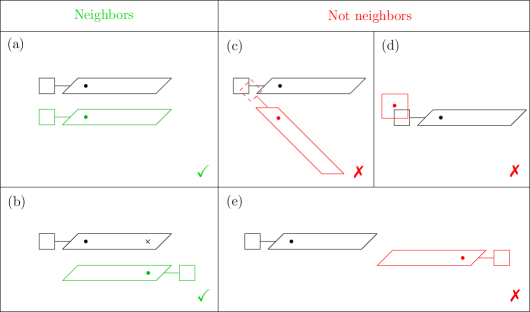
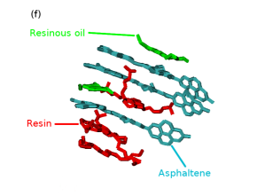
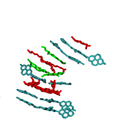
The definition of a nanoaggregate is described in detail in Ref. [aging, ]. It is based on the following rule: two aromatic molecules are nearest neighbors in the same nanoaggregate if they are ”well-aligned” and ”close enough”. A nanoaggregate is composed of all molecules connected by this rule. Moreover, the asphaltene molecule chosen in this model has two parts, a flat head and a flat body which can rotate with respect to each other. For this reason, aromatic molecules can align in the direction of an asphaltene body or in the direction of an asphaltene head, thus creating branched nanoaggregates. These branches can link together purely linear nanoaggregates. We believe this is one mechanism explaining the formation of clusters of nanoaggregates, also observed experimentally [mullins2012, ]. In this paper, we focus on purely linear nanoaggregates. It means that any aromatic molecules linked to an asphaltene head will not be considered as part of this asphaltene nanoaggregate. We define a linear aggregate as composed of asphaltene bodies, resin and resinous oil molecules, and not asphaltene heads because heads are the smallest parts and probably lead to the smallest interaction energy. Figure 2 shows conformations of two molecules corresponding to limiting cases of the nanoaggregate definition used in this paper. Figures 2(a) and (b) show two conformations of two asphaltene molecules where these molecules are considered as nearest neighbors. Conversely, Figs 2(c) to (e) show three conformations where the two molecules are not considered as nearest neighbors. A picture of a linear nanoaggregate obtained from the MD simulations is shown in Fig. 2(f). Note that this nanoaggregate is not typical as a resin and a resinous oil molecule are aligned on the same side of an asphaltene body.

Figure 2: (Color online) (a) to (e) Scheme of limiting cases illustrating whether a molecule is or is not the nearest neighbor of the first molecule. The first molecule is an asphaltene molecule and is black. The second molecule is green if it is the neighbor of the first one and red otherwise. (a) Head-to-head conformation. (b) Head-to-tail conformation. (c) Non-aligned molecules. (d) Molecule aligned to the head of the asphaltene molecule. (e) Molecules far from each other and aligned. Modified with permission from C. A. Lemarchand, T. B. Schroder, J. C. Dyre, and J. S. Hansen, J. Chem. Phys. 139, 124506 (2013). Copyright 2013 American Institute of Physics. (f) Snapshot of a linear nanoaggregate, obtained in molecular dynamics. Asphaltene molecules are in blue, resin molecules in red and resinous oil molecules in green.

II.3 Probability of having a nanoaggregate of a given size

Sections II.1 and II.2 gave necessary information about the simulations and the definition of linear nanoaggregates. The results of the molecular dynamics simulations concerning the nanoaggregate size and stability can now be presented.

There are different possibilities to quantify the size of a linear nanoaggregate. For example, it can be quantified as the total number of aromatic molecules or as the number of asphaltene molecules which it contains. The first definition makes use of the fact that nanoaggregates are not only composed of asphaltene molecules, but also of smaller aromatic molecules. The second definition accounts for the fact that asphaltene molecules are the largest aromatic molecules and probably the most important in the nanoaggregate stability. This is why experimentalists often define the nanoaggregate size as the latter [mullins2012, ].

The molecular dynamics simulations enable us to study the consequences of both definitions on the nanoaggregate stability. We quantify the stability as the probability of having a nanoaggregate of a given size in the stationary regime. The probability $P_{\text{mol}}(n)$ of having a nanoaggregate containing $n$ aromatic molecules is defined as:

$$P_{\text{mol}}(n)=\frac{N_{n,\text{mol}}}{N_{t}},$$ (1)

where $N_{n,\text{mol}}$ is the number of linear aggregates containing $n$ aromatic molecules and $N_{t}$ is the total number of linear aggregates. In a similar way, the probability $P_{X}(n)$ of having a nanoaggregate with $n$ molecules of type $X$ is defined as

$$P_{X}(n)=\frac{N_{n,X}}{N_{t,X}},$$ (2)

where $N_{n,X}$ is the number of linear aggregates containing $n$ molecules of type $X$ and $N_{t,X}$ is the total number of linear aggregates containing at least one molecule of type $X$. The type $X$ can be $A$ for asphaltene, $R$ for resin, $RO$ for resinous oil or $RRO$ for resin and resinous oil. The probabilities $P_{A}(n)$ and $P_{RRO}(n)$ are plotted in Fig. 3 (b) and (c), respectively. The probabilities $P_{R}(n)$ and $P_{RO}(n)$ are plotted in Fig. 3 (d). Two main points can be noticed in Fig. 3. The probability $P_{\text{mol}}$ of having a nanoaggregate containing $n$ aromatic molecules seems to have two slopes in a log-lin scale, i. e. can be described by a biexponential. On the contrary, when only asphaltene molecules are counted, the probability $P_{A}$ has only one slope, i. e. can be characterized as a simple exponential. For the probability $P_{RRO}$ of having a nanoaggregate containing $n$ resin or resinous oil molecules, the biexponential shape seems to be prevailing. It is the same for the probability $P_{R}$ of having a nanoaggregate containing $n$ resin molecules. For the probability $P_{RO}$ of having a nanoaggregate containing $n$ resinous oil molecules, the monoexponential shape seems to be recovered. The transition between the two slopes is not sharp for the probability $P_{R}$. To highlight the existence of the two slopes in this case in Fig. 3 (d), a dashed line was drawn in continuation of the line corresponding to the first slope. It departs further and further away from the second slope.

Figure 3: (Color online) (a) Probability $P_{\text{mol}}(n)$ of having a nanoaggregate containing $n$ aromatic molecules versus $n$. (b) Probability $P_{A}(n)$ of having a nanoaggregate containing $n$ asphaltene molecules versus $n$. (c) Probability $P_{RRO}(n)$ of having a nanoaggregate containing $n$ resin or resinous oil molecules versus $n$. (d) Probability $P_{R}(n)$ of having a nanoaggregate containing $n$ resin molecules versus $n$ and probability $P_{RO}$ of having a nanoaggregate containing $n$ resinous oil molecules versus $n$. In every case the straight lines (orange or green) are guides to the eye. They highlight the monoexponential behavior in the subfigures (b) and (d), when resinous oil molecules are counted, and the biexponential behavior in the subfigures (a), (c), and (d), when resin molecules are counted. The error bars correspond to the standard deviation estimated from eight independent simulations.

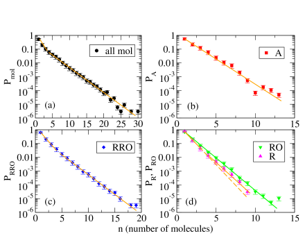
The rest of the paper is devoted to understand the molecular dynamics results presented in Fig. 3. More specifically, the paper is aimed at unraveling some of the dynamical and thermodynamical origins lying behind the monoexponential and biexponential behaviors. A dynamical approach will first be proposed for the monoexponential behavior.

III Dynamical approach

In Fig. 3 (b), the probability of having a nanoaggregate containing $n$ asphaltene molecules was shown to be monoexponential. The aim of this section is to establish a simple aggregation mechanism reproducing this behavior. The mechanism will be used to derive a master equation which provides a dynamical framework for understanding the monoexponential behavior.

A simple mechanism which can be written in the asphaltene aggregation problem is

$$A_{n}+A_{1}\rightleftharpoons A_{n+1},\quad n=1,2,...$$ (3)

where $A_{n}$ denotes an aggregate containing $n$ asphaltene molecules. The assumptions lying behind this mechanism are the following: only one asphaltene molecule at a time can attach to or detach from an existing aggregate, the medium is homogeneous and the aggregation dynamics is not limited by diffusion. The same mechanism was already suggested in Ref. [aguilera2006, ] to model asphaltene aggregation from a thermodynamical point of view, but the possibility to obtain a master equation from this mechanism and consequently to model the dynamics of asphaltene aggregation was left aside.

To obtain a master equation linked to this aggregation reaction, we make supplementary assumptions: the reaction rate constants do not depend on the size $n$ of the aggregate and the attachment rate does not depend on the probability of having free asphaltene molecules in the medium. Under these assumptions, the master equation linked to the aggregation reaction Eq. (3) can be written as:

$$\frac{dP_{A}(1,t|n_{0})}{dt} =\mu P_{A}(2,t|n_{0})-(\lambda+\mu)P_{A}(1,t|n_{0})+\mu-\lambda,$$ (4)

$$\frac{dP_{A}(n,t|n_{0})}{dt} =\lambda P_{A}(n-1,t|n_{0})+\mu P_{A}(n+1,t|n_{0})-(\lambda+\mu)P_{A}(n,t|n_{0}),\quad\text{for}\quad n=2,3,...$$ (5)

where $\lambda$ is the attachment rate constant, $\mu$ the detachment rate constant and $P_{A}(n,t|n_{0})$ the probability of having an aggregate containing $n$ asphaltene molecules at time $t$, given that its initial size was $n_{0}$. The probability denoted $P_{A}(n)$ in Sec. II.3 corresponds to the stationary state to Eqs. (4) and (5) and depends neither on time $t$ nor on the initial condition $n_{0}$. The master equation Eq. (5) was solved analytically in the 1950’s [morse55, ,schwarz75, ] for different boundary conditions. This master equation and its generalized version in which the rate constants depend on the aggregate size $n$ have also been extensively used to model different stochastic processes such as alcohol clusters [sillrenMasterEq, , thesisPer, ], biological adhesion clusters [erdmann, ] or aggregation in freeway traffic [mahnke, ], to cite only a few.

The expression of this master equation deserves some further clarification in connection to the specific aggregation reaction used. Following the law of chemical kinetics, the attachment rate linked to the aggregation mechanism (3) should be $\lambda P_{A}(n-1,t|n_{0})P_{A}(1,t|n_{0})$, because the probability of having a collision between two small spherical molecules is usually proportional to the product of their concentrations. We can give empirical reasons explaining why it is not proportional to the probability $P_{A}(1,t|n_{0})$ of having a free asphaltene molecule here. We assume that the attachment rate is not due to the collision between two small spherical molecules, but limited by the steric hindrance around the aggregate and the orientation of the free asphaltene molecule $A_{1}$. The attachment reaction is successful if the free asphaltene molecule is well oriented and placed at a reactive end of the aggregate. The number of free asphaltene molecules is higher than the number of any aggregate of a given size at any time in our MD simulations (not shown). As the number of free asphaltene molecules is high enough, there is always a free asphaltene molecule nearby an aggregate but it is not always well-oriented and prevent other molecules from approaching due to the density of the system. Thus, the attachment rate is independent of the free asphaltene concentration and the attachment rate constant $\lambda$ is averaged over possible orientations. The boundary condition Eq. (4) needs also some explanation. It corresponds to the fact that the system is closed. In other words, the total number of asphaltene molecules is kept constant. As the free asphaltene molecules are involved in each aggregation reaction (3), the derivative with respect to time of the probability $P(1,t|n_{0})$ to have a free asphaltene molecule depends on infinitely many terms. It leads to

$$\frac{dP_{A}(1,t|n_{0})}{dt}=2\mu P_{A}(2,t|n_{0})-2\lambda P_{A}(1,t|n_{0})+\sum\limits_{n=3}^{\infty}\mu P_{A}(n,t|n_{0})-\sum\limits_{n=2}^{\infty}\lambda P_{A}(n,t|n_{0}).$$ (6)

These series are then simplified using the fact that at every time $t$: $\Sigma_{n=1}P_{A}(n,t|n_{0})=1$, to give the boundary condition Eq. (4).

To test the validity of this master equation for the present problem, two different quantities are evaluated : the stationary probability of having a nanoaggregate of a given size, as shown in Sec. II.3 and the aggregation dynamics, quantified as the time evolution of the fraction of aggregated asphaltene molecules.

III.1 Stationary regime

The stationary distribution of the master equation Eq. (5) with the boundary condition Eq. (4) is easy to derive. In the stationary state, the probability of having a nanoaggregate containing $n$ asphaltene molecules depends neither on time nor on the initial size of a nanoaggregate. For this reason, the stationary probability will be denoted $P_{A}(n)$. It satisfies the following equation:

$$(\lambda+\mu)P_{A}(1)=\mu P_{A}(2)+\mu-\lambda,$$ (7)

$$\lambda P_{A}(n-1)+\mu P_{A}(n+1)-(\lambda+\mu)P_{A}(n)=0,\quad\text{for}\quad n=2,3,...$$ (8)

The solution of this equation is a geometrical law [morse55, , schwarz75, ]. By induction and using the fact that $\Sigma_{n=1}^{\infty}P_{A}(n)=1$, one can show that the solution of this equation is:

$$P_{A}(n)=p^{n-1}(1-p),\quad\text{where}\quad p=\frac{\lambda}{\mu}.$$ (9)

In a log-lin scale, the stationary probability predicted by the master equation approach is a straight line of the form :

$$\ln(P_{A}(n))=\ln(p)n+\ln\Bigl{(}\frac{1-p}{p}\Bigr{)}.$$ (10)

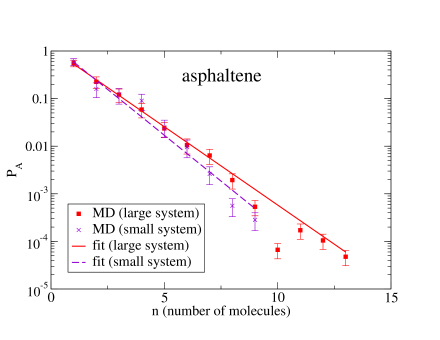
It is a monoexponential distribution, as observed in Fig. 3 (b), obtained in MD. The exponential distribution can be used to fit the molecular dynamics data, as shown in Fig. 4. The value of the dynamical parameter $p$ is, in this case, $p=0.44$. The master equation framework provides a dynamical interpretation of the parameter $p$ as the ratio between the attachment and detachment rate constants.

Figure 4 also shows the probability of having a nanoaggregate containing $n$ asphaltene molecules obtained in MD simulations for two different system sizes and the corresponding exponential fits. The results for a system containing $50$ asphaltene molecules and for a system containing $5$ times less molecules agree surprisingly well, giving the values $p=0.44$ and $p=0.41$ respectively. It shows that, while finite size effects are present, they are not very important when it comes to the number of asphaltene molecules in a nanoaggregate. More specifically, the relative probability of small nanoaggregates is accurately described even in the small system. The probability of having larger nanoaggregates is not so well described in the small system, as expected, but does not affect much the value of the parameter $p$ since these nanoaggregates are rare even in the large system. It is important to note, however, that physical properties due to large nanoaggregates or to nanoaggregates filling up the box in one direction, such as residual stresses, could be affected by finite size effects.

Figure 4: (Color online) Probability of having a nanoaggregate containing $n$ asphaltene molecules versus $n$. Data for a large system, containing $50$ asphaltene molecules, $50$ resin molecules, $50$ resinous molecules and $410$ docosane molecules and for a system $5$ times smaller are shown. The results for the large system were already shown in Fig. 3 (b). The red solid line is a fit of Eq. (9) to the data of the large system, with $p=0.44$. The purple dashed line is a fit of Eq. (9) to the data of the small system, with $p=0.41$.

III.2 Aggregation dynamics

As shown above, the stationary state predicted by the master equation agrees with the MD results on the probability of having a nanoaggregate containing $n$ asphaltene molecules. If the master equation Eq. (5) correctly describes the aggregation process, it should also reproduce the aggregation dynamics. Checking this fact is the purpose of this section.

To compare the prediction of the master equation approach and the molecular dynamics results, we quantified the aggregation dynamics in the following way. We used the fraction $f_{a}$ of aggregated asphaltene molecules versus time. The fraction $f_{a}$ of aggregated asphaltene molecules is defined as the ratio of the number of asphaltene molecules in all aggregates containing at least two asphaltene molecules and the total number of asphaltene molecules in the system. The fraction $f_{a}$ verifies:

$$f_{a}=1-f_{1},$$ (11)

where $f_{1}$ is the fraction of free asphaltene molecules. The fraction of free asphaltene molecules is defined as

$$f_{1}=\frac{M_{1,A}}{M_{t,A}},$$ (12)

where $M_{1,A}$ is the number of asphaltene molecules in aggregate containing one asphaltene molecule and $M_{t,A}$ is the total number of asphaltene molecules in the system. The fraction $f_{1}$ can be expressed in terms of the probability $P(1,t|1)$ of having an asphaltene aggregate of size $1$ at time $t$ and of the average size of an asphaltene aggregate $\langle n\rangle_{1}(t)$, given that all aggregates had size 1 initially. Indeed, we know that:

$$P_{A}(1,t|1)=\frac{N_{1,A}}{N_{t,A}},$$ (13)

where $N_{1,A}$ is the number of aggregates containing one asphaltene molecule and $N_{t,A}$ is the total number of aggregates containing at least one asphaltene molecule, as in Eq. 2. We also know that:

$$\langle n\rangle_{1}(t)=\frac{M_{t,A}}{N_{t,A}},$$ (14)

where $M_{t,A}$ is again the total number of asphaltene molecules and $N_{t,A}$ is the total number of aggregates containing at least one asphaltene molecule. It is easy to show that $N_{1,A}=1\times M_{1,A}$ and finally that

$$f_{1}=\frac{P_{A}(1,t|1)}{\langle n\rangle_{1}(t)}.$$ (15)

To obtain the dynamics predicted by the master equation Eq. (5) with the specific boundary condition Eq. (4), a numerical implementation of the scheme was carried out. In the numerical implementation the time step $\Delta t$ is a hundred times smaller than the inverse of the detachment rate constant $1/\mu$. An aggregate can attach to a single molecule with the probability $\lambda\Delta t$ and release a single molecule with the probability $\mu\Delta t$. An aggregate of size $1$ can attach to a molecule but cannot release one. The total number of molecules is kept constant in the numerical implementation of the master equation. The total number of molecules is chosen to be $5000$ to reduce the statistical noise. Initially, in the numerical implementation of the master equation, all the aggregates are of size $1$.

The fraction $f_{1}$ of free asphaltene molecules can be obtained through this numerical implementation. It depends a priori on the two rate constants $\lambda$ and $\mu$. However, the ratio $p=\lambda/\mu$ is known from the stationary state result. It leaves us with one dynamical parameter, say $\lambda$, to fit. The initial state in the molecular dynamics simulations is not as well defined as in the master equation approach. To reach the desired density, a first MD simulation where the system is compressed is performed. During the compression period, the asphaltene molecules begin to aggregate, but the data cannot be recorded. The data are recorded just after the compression period, in a state where small asphaltene aggregates are already formed. The fraction of free asphaltene molecules in that state is $f_{1i}=0.36$. It is a second fitting parameter. The curve predicted by the numerical implementation of the master equation was shifted in time so that time $t=0$ corresponds to $f_{1i}=0.36$ as in the MD simulations. Figure 5 shows the fraction of aggregated asphaltene molecules versus time in the molecular dynamics simulations and in the master equation approach. Both results agree well, indicating that the master equation approach correctly describe the aggregation process of asphaltene molecules. The value of the dynamical parameter $\lambda$ is found to be $\lambda=4.4\cdot 10^{7}$ s^-1.

It is worth mentioning that the inverse rate constant $1/\lambda=2.3\cdot 10^{-8}$ s is much larger than the upper limit $\tau=5.3\cdot 10^{-10}$ s, needed for an asphaltene molecule to diffuse of a distance equals to the average distance $d=1.34$ nm between the centers of mass of $150$ aromatic molecules in a homogeneous system of volume $362$ nm³ minus the intermolecular distance $d_{\text{avg}}=4$ Å in an aggregate. This characteristic time is evaluated using the diffusion coefficient of a single asphaltene molecule in the docosane solvent: $D=2.8\cdot 10^{-10}$ m².s^-1 and the formula $\tau=(d-d_{\text{avg}})^{2}/(6D)$ for three-dimensional diffusion. This time is an upper limit because only the distance between centers of mass is considered, whereas molecules are extended in space and can be close to each other even if the distance between their centers of mass is larger than $d_{\text{avg}}$. We can conclude from that fact that the nanoaggregation process is not limited by diffusion.

In Fig. 5, there seems to be a discrepancy between the master equation approach and the MD results at long times. This could indicate the existence of another aggregation process, taking place at a longer time scale. Checking carefully the existence of this second process requires further investigation.

Figure 5: Time evolution of the fraction of aggregated asphaltene molecules $f_{a}$ in molecular dynamics simulations and in the master equation approach.

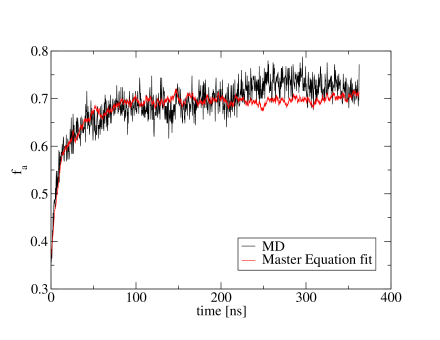
The master equation approach related to the aggregation reaction Eq. (3) is able to reproduce both the stationary behavior and the dynamics of the asphaltene aggregation process at intermediate time scales. It indicates that the assumptions made to derive the master equation Eq. (5) are relevant. The master equation approach gives a dynamical framework to interpret the monoexponential distribution observed in MD. Even if the same master equation has already been used in the general field of clustering processes [sillrenMasterEq, ; erdmann, ; mahnke, ], it is the first time, to our knowledge, that it is applied to asphaltene aggregation in molecular dynamics simulations.

IV Statistical mechanics approach

Section III provided a dynamical interpretation of the monoexponential behavior of the probability of having a nanoaggregate containing $n$ asphaltene molecules based on a master equation description on a simple aggregation reaction. The aim of the present section is to describe a statistical mechanics model based on the same aggregation scheme and consistent with the monoexponential behavior. In this section, we will also look into possible thermodynamical interpretations of the biexponential behavior, obtained when all aromatic molecules are counted.

IV.1 Statistical mechanics model

To formulate a simple statistical mechanics model linked to the aggregation reaction Eq. (3), some assumptions are needed. We make the following common assumptions:

1. The nanoaggregates are linear.

2. The system is homogeneous and isotropic on average and the nanoaggregates are rigid.

3. The aggregation process occurs at a characteristic time much larger than the equilibration of the pressure, temperature and solvent molecules.

4. The system is dilute enough to consider no interaction between the nanoaggregates except through the aggregation reaction. In other words, the solution of nanoaggregates of different sizes in a solvent is ideal.

5. The free energy of a nanoaggregate depends linearly on its size.

The idea of considering a mixture of free molecules and dimers as an ideal mixture with an aggregation reaction occurring at a larger time scale dates back to the beginning of the 20${}^{\text{th}}$ century [dolezalek1908, ; dolezalek1910, ] as is nicely explained in the recent review [gubbins, ]. The set of assumptions was then completed to include the case of linear aggregates of any size and widely used to describe rodlike micelles [cates1991, ], linear polymer chains [wittmer98, ; wittmer2000, ], and discotic liquid crystals [hurt, ]. We propose in this section our own version of the derivation applied to the case of linear asphaltene aggregates and obtain an analytical formula for the probability of having an aggregate of a given size. The analogy between linear assembly in discotic liquid crystals and asphaltene aggregates was also made in Ref [aguilera2006, ], which derives very similar equations to the ones presented in this section, but do not present a successful comparison with their coarse-grained simulations of asphaltene-resin nanoaggregates at high density.

The assumption of having an ideal mixture can be relaxed to take into account more complicated interactions between the aggregates such as excluded volume interactions [doi, ; vanderSchoot, ], the gain in entropy when the chain breaks [wittmer98, ] and interactions due to the flexibility of the aggregates[khokhlov, ; kuriabova, ; demichele, ], to cite only a few. For the sake of simplicity, these interactions are neglected in the case of linear asphaltene aggregates. The validity of the assumptions made in this section will be discussed in Sec. IV.2.

Concurrently to these approaches expressing the probability of having an aggregate of a given size, another theory of aggregation based on statistical thermodynamics was developed by Wertheim [wertheim, ; gubbins, ]. This theory considers molecules of a reference liquid, typically a Lennard-Jones fluid, with a finite number of binding sites. The potential modeling the interaction between the binding sites is designed to take into account steric hindrance. The theory then counts the number of molecules with no bond on a given binding site instead of the number of aggregates of a given size. It is a clever way to count physically meaningful graphs. The outcome of the theory is an expression for the equilibrium pressure and the concentration of free molecules versus the composition of the system. These predictions were successfully checked numerically for strongly associating fluid [johnson, ]. However, this theory does not provide an expression for the probability of having an aggregate of a given size. For this reason, it is not considered in further details in this section but is mentioned for the sake of completeness.

In the framework of the common assumptions stated above, the free energy of the system can be written as [Diu, ]:

$$F=\sum\limits_{n}k_{B}T\Bigl{(}N_{n,A}(\ln(N_{n,A})-1)-N_{n,A}\ln(V)\Bigr{)}+N_{n,A}F_{e}^{(n)},$$ (16)

where $N_{n,A}$ is the number of nanoaggregates containing $n$ asphaltene molecules, $V$ the volume of the system, $F_{e}^{(n)}$ the effective free energy of an aggregate, $k_{B}$ the Boltzmann constant and $T$ the temperature. The first term in Eq. (16) corresponds to the free energy of an ideal mixture of ideal gas and the second term corresponds to the energy of the aggregates. The effective free energy $F_{e}^{(n)}$ is to be understood as the energy of an asphaltene aggregate when the degrees of freedom due to solvent molecules have been integrated out.

The expression Eq. (16) for the free energy of the system holds for each value of the number $N_{n,A}$ of aggregates of a given size, because a state of local equilibrium acting on entropy, pressure and solvent molecules is assumed for each step along the aggregation reactions. The total equilibrium of the system depends now only on the equilibrium of the aggregation reactions (3). The condition for chemical equilibrium of each aggregation reaction $A_{n}+A_{1}\rightleftharpoons A_{n+1}$ is

$$\mu_{n+1}-\mu_{n}-\mu_{1}=0,\quad\text{for }n=1,2,...$$ (17)

where $\mu_{n}$ is the chemical potential of an asphaltene aggregate of size $n$. Using the definition of the chemical potential $\mu_{n}=\partial F/\partial N_{n,A}$, we can obtain after some calculations the well-known mass action law:

$$\frac{N_{n+1,A}}{N_{n,A}N_{1,A}}=\frac{K_{n}(T)}{V},\quad\text{for}\quad n=1,2,...$$ (18)

where $K_{n}(T)$ is the equilibrium constant of the reaction $A_{n}+A_{1}\rightleftharpoons A_{n+1}$. The equilibrium constant is given by:

$$K_{n}(T)=\exp\Bigl{(}-\frac{F_{e}^{(n+1)}-F_{e}^{(n)}-F_{e}^{(1)}}{k_{B}T}\Bigr{)}.$$ (19)

We now make use of assumption 5, stating that the free energy of a nanoaggregate depends linearly on its size. This assumption amounts to write the effective free energy $F_{e}^{(n)}$ as:

$$F_{e}^{(n)}=nF_{0}+(n-1)F_{e},$$ (20)

where $F_{0}$ is the free energy of a single asphaltene molecule and $F_{e}$ is the effective free energy between two asphaltene molecules. Using this form in the expression of the equilibrium constant Eq. (19) gives:

$$K(T)=\exp\Bigl{(}-\frac{F_{e}}{k_{B}T}\Bigr{)}.$$ (21)

Thus, the equilibrium constant does not depend on the size $n$ of the considered nanoaggregate under the set of assumptions considered. By induction, it is now easy to show from Eq. (18) that

$$N_{n,A}=N_{1,A}^{n}\Bigl{(}\frac{K(T)}{V}\Bigr{)}^{n-1}.$$ (22)

To compare the model to the simulations results it is more useful to obtain the probability $P_{A}(n)$ of having a nanoaggregate of size $n$, which is defined in Eq.2

$$P_{A}(n)=\frac{N_{n,A}}{N_{t,A}},$$ (23)

where $N_{t,A}=\sum_{n}N_{n,A}$ is the total number of asphaltene nanoaggregates. To express $P_{A}(n)$, we make use of the conservation of the total number $M_{t,A}$ of asphaltene molecules:

$$M_{t,A}=\sum\limits_{n}nN_{n,A}.$$ (24)

Having this in mind, one can show (see Appendix A) that

$$P_{A}(n)=p^{n-1}(1-p)$$ (25)

where

$$p=\frac{x+1-\sqrt{2x+1}}{x},$$ (26)

and

$$x=\frac{2M_{t,A}}{V}\exp\Bigl{(}-\frac{F_{e}}{k_{B}T}\Bigr{)}.$$ (27)

We have now recovered the exponential distribution observed in the MD simulations and Fig. 3 (b). The MD simulations provide a value of the parameter $p$ characterizing the exponential distribution: $p=0.44$. According to the thermodynamical interpretation Eq. (26), it leads to the value

$$F_{e}=-4.0\text{ }k_{B}T.$$ (28)

The simple statistical mechanics model provides an interpretation for the parameter $p$ in terms of an effective free energy $F_{e}$ between two asphaltene molecules. Within the assumptions of this simple model, the effective free energy is the interaction energy between two asphaltene molecules when the degrees of freedom related to solvent molecules are integrated out.

The physical meaning of free energy $F_{e}$ depends on its definition in the framework of the assumptions made here, but also on the validity of these assumptions. This will be discussed in the next section.

IV.2 Physical meaning of the effective free energy and validity of the assumptions

The validity of each assumption and its consequences on the physical meaning of the free energy $F_{e}$ will now be listed.

1. Linear dependence of $F_{e}^{(n)}$ on the size $n$ of the nanoaggregate.

   It is very easy to check that the potential energy, and not the free energy, of a nanoaggregate in vacuum depends linearly on its size. The potential energy of a linear nanoaggregate of size $n$ is plotted versus $n$ for nanoaggregates in vacuum in Fig. 6. The origin of the energy is set arbitrarily to zero in this figure. The nanoaggregate used to plot this figure is a linear nanoaggregate containing five asphaltene molecules found in one simulation. To find the potential energy of an aggregate of size $n\leq 5$, only the first $n$ asphaltene molecules in the aggregate were considered in vacuum. This figure clearly shows that the potential energy of a nanoaggregate in vacuum is linear and the slope $U_{\text{vacuum}}$ corresponding to the interaction energy between two asphaltene molecules is equal to

   $$U_{\text{vacuum}}=-87\text{ }k_{B}T.$$ (29)

   In practical terms, it means that when an asphaltene molecule is added to a nanoaggregate of size $n$, this asphaltene molecule interacts with the energy $-87$ $k_{B}T$ with the molecule at the end of the nanoaggregate but do not interact with the other ones, which are further away.

   

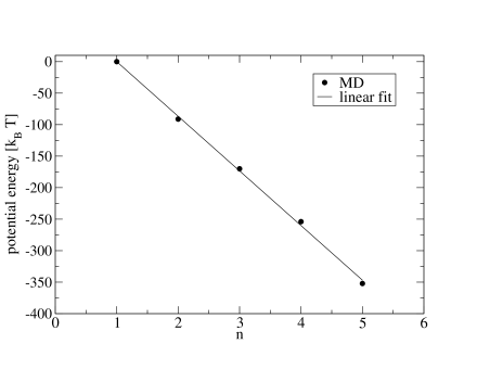
   Figure 6: Potential energy of a linear asphaltene nanoaggregate in vacuum versus the number $n$ of asphaltene molecules which it contains.

   The fact that the potential energy of a nanoaggregate in vacuum depends linearly on its size is a good indication that it might also be the case for the effective free energy $F_{e}^{(n)}$ of a nanoaggregate in a solvent. In that case, the effective free energy $F_{e}$ corresponding to the slope of $F_{e}^{(n)}$ versus the size $n$ of the nanoaggregate is well defined.

   We remind the reader that the potential energy of a nanoaggregate in vacuum and the effective free energy $F_{e}^{(n)}$ are not identical and the slopes $F_{e}$ and $U_{\text{vacuum}}$ are indeed quite different. Within the framework of the statistical model presented in Sec. IV.1, the two causes of this difference are: the interaction between the asphaltene molecules and the solvent and the entropic effects due to the effective integration of the degrees of freedom of the solvent. To quantify the effective free energy $F_{e}$ properly, a possibility is to set up umbrella sampling simulations controlling the distance between the center of mass of two asphaltene molecules in a bath of docosane molecules at the same temperature and pressure as the one used in the MD simulations. The free energy of this system can be derived in terms of the distance between the two asphaltene molecules. The effective free energy $F_{e}$ would then be the difference between the free energy of such a system when the two asphaltene molecules are far away and the free energy of the system when the two asphaltene molecules are aligned and close. Implementing umbrella sampling simulations is beyond the scope of this paper. Moreover, the free energy $F_{e}$ found with this method might be slightly different from the value $F_{e}=-4.0$ $k_{B}T$, found using the statistical mechanics model of Sec. IV.1, because of the other assumptions made to derive this model.

2. Asphaltene nanoaggregates.

   To derive the statistical mechanics model in Sec. IV.1, we only considered the aggregation of asphaltene molecules, whereas resin and resinous oil molecules are also part of the nanoaggregates. The degrees of freedom related to the position of resin and resinous oil molecules should be integrated in an effective way to obtain the free energy $F_{e}$, just as it was done for the degrees of freedom related to the solvent. The fact that the monoexponential behavior is valid for the probability of having a nanoaggregate containing $n$ asphaltene molecules means that this effective integration can be done.

3. Linear nanoaggregates.

   The nanoaggregates considered in the simulations are only some linear portions of bigger branched nanoaggregates. The existence of the branches could also produce some degrees of freedom to be integrated to obtain the effective free energy $F_{e}$.

4. Dilute limit.

   The assumption stating that the solution of nanoaggregates is ideal neglects the interaction between the nanoaggregates. Some of these interactions, for example between the nanoaggregates $A_{n}$, $A_{n+1}$ and $A_{1}$, are later taken into account through the aggregation reactions (3) corresponding to the asphaltene aggregation. But in the MD simulations, the asphaltene molecules interact in a more complicated way. They cannot for example be too close to each other, due to short range repulsion. This could be taken into account through excluded volume interactions. It is known [vanderSchoot, , kuriabova, ], that taking into account excluded volume interactions preserves the monoexponential behavior. Consequently, excluded volume interactions might play a role in the value of the effective free energy $F_{e}$.

5. Time scale of the aggregation reactions.

   To derive the statistical mechanics model, we assumed that the aggregation reactions occurred on a time scale much larger than the time scale associated with the equilibrium of pressure, entropy, and solvent molecules for a given number of each nanoaggregate. It is very difficult to predict the effect of the relaxation of this fundamental assumption. One way to check the assumption, however, is to compare once again the characteristic time of the aggregation reaction $1/\lambda=2.3\cdot 10^{-8}$ s and the upper limit $\tau=5.3\cdot 10^{-10}$ s for the diffusion of an asphaltene molecule. A factor $20$ exists between the two characteristic times which should be enough to ensure the validity of the assumption.

6. Rigidity of the nanoaggregates and isotropy of the system.

   The assumptions of rigid nanoaggregates and isotropic system can be considered together, because if they are both relaxed, they lead to a new term in the free energy of the system [lu2004, ; lu2006, ; kuriabova, ]. This term depends on a persistence length $l_{p}$ and reads as [khokhlov, ,kuriabova, ]

   $$F_{\text{flexible}}=-V\frac{2L}{3l_{p}}\sum\limits_{n}\int\frac{d\Omega_{\mathbf{u}}}{4\pi}[\rho_{n}(\mathbf{u})]^{1/2}\nabla[\rho_{n}(\mathbf{u})]^{-1/2},$$ (30)

   where

   $$\rho_{n}(\mathbf{u})=\frac{nN_{n}}{V}$$ (31)

   is the number density of asphaltene molecules part of a nanoaggregate of size $n$ oriented in the direction $\mathbf{u}$ with respect to some reference direction and $\Omega_{\mathbf{u}}$ is the corresponding solid angle. This term is helpful to describe the nematic phase of liquid crystals, where long range order is seen. The addition of this term in the free energy expression leads to a biexponential behavior [lu2004, ; lu2006, ; kuriabova, ], which is not observed for the probability of having a linear nanoaggregates with $n$ asphaltene molecules. Consequently, the assumption of rigid nanoaggregates and isotropic system probably holds, at least in an effective way, for the probability of having a linear nanoaggregate with $n$ asphaltene molecules and does not participate in the value of the effective free energy $F_{e}$. The addition of this flexible term to the free energy is potentially of interest to explain the biexponential behavior of the probability of having a nanoaggregate containing $n$ aromatic molecules.

To summarize, one can say that the statistical mechanics model developed in Sec. IV.1 provides a thermodynamical interpretation of the monoexponential behavior based on the effective free energy between two asphaltene molecules. This effective free energy should be understood as the interaction energy between two asphaltene molecules when all the degrees of freedom related to solvent molecules, resin and resinous oil molecules and branched nanoaggregates have been integrated out.

IV.3 Biexponential behavior

The picture emerging from the study of the probability of having a linear nanoaggregate containing $n$ asphaltene molecules is that asphaltene bodies interact with an effective energy through the aggregation reaction (3). This leads to a monoexponential behavior. We know that the probability of having a linear nanoaggregate with $n$ aromatic molecules has a different behavior. It is biexponential as shown in Fig. 3 (a). This section is devoted to identifying possible statistical mechanics explanations for this different behavior.

IV.3.1 Role of resin and resinous oil molecules

The first explanation that comes to mind is that when all molecules are counted, different interaction energies are involved. Each interaction energy taken separately would lead to a specific monoexponential behavior and the combinations of several interaction energies could lead to a bi- or multiexponential behavior.

To test this idea, we set up one-dimensional lattice Monte-Carlo simulations. A linear lattice of $N$ sites is created. Each site can contain one asphaltene molecule, one resin molecule, one resinous oil molecule or nothing. One site cannot contain two molecules. The total numbers of asphaltene molecules, resin molecules, and resinous oil molecules are constant. A Monte-Carlo move consists in exchanging the content of two sites providing that the content is different. This condition makes the molecules indiscernible. The system is initialised with the largest possible aggregate where all asphaltene molecules are next to each other, then comes resin molecules and then resinous oil molecules. Ten million ($10^{7}$) Monte-Carlo moves are realised using the Metropolis algorithm. The algorithm converges quite quickly despite its elementary implementation. The potential energy of a nanoaggregate is calculated in the following way: when two asphaltene molecules are next to each other the interaction $u_{A}$ between two asphaltene molecules is added, when a resinous oil molecule is next to an asphaltene molecule or another resinous oil molecule the interaction energy $u_{RO}$ is added, finally when a resin molecule is next to any other molecule the interaction energy $u_{R}$ is added. As two molecules cannot be on the same site, effective excluded volume interactions are created. The assumptions underlying the establishment of the one-dimensional lattice Monte-Carlo simulations are similar to the ones made in Sec. IV.1 except for excluded volume interactions:

1. The nanoaggregates can only be linear because the system is one-dimensional.

2. The nanoaggregates are rigid. The system is one dimensional, so isotropy is not a criterion.

3. The only energies involved are those related to the aggregation process. All potential energies related to interaction with and within solvent molecules are averaged out. No kinetic energy is involved.

4. The system is not dilute and excluded volume interactions are taken into account.

5. The energy of a pure asphaltene nanoaggregate depends linearly on its size.

One of the main advantages of lattice Monte-Carlo simulations compared to the analytical approach is to take into account resin and resinous oil molecules and not only asphaltene molecules. We checked that in the dilute limit, when only asphaltene molecules are present in the Monte-Carlo simulations, the same monoexponential behavior with the same value for the parameter $p$ as the one predicted by the analytical approach is recovered.

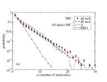
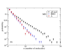
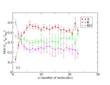
In the lattice Monte-Carlo simulations, it is possible to obtain a biexponential behavior for the probability of having $n$ molecules in a nanoaggregate as can be seen in Fig. 7a. The biexponential behavior is characterized by the presence of two straight lines with different slopes in a log-lin scale. The biexponential behavior occurs in the lattice Monte-Carlo simulations when the interaction energies $u_{A}$ between asphaltene molecules on the one hand and $u_{RO}$ and $u_{R}$ with resin and resinous oil molecules on the other hand are substantially different. For example, the choices $u_{A}=-5$ $k_{B}T$, $u_{RO}=-2.7$ $k_{B}T$ and $u_{R}=-2.3$ $k_{B}T$ at the same temperature and same volume as the MD simulations give a biexponential behavior very close to the one obtained in MD in Fig. 3 (a). It is shown in Fig. 7 (a). However, the biexponential behavior does not have the same causes as in the MD simulations. In the Monte-Carlo simulations, the biexponential behavior is due to the fact that pure resin or resinous oil nanoaggregates and pure asphaltene nanoaggregates are formed. There are very few mixed nanoaggregates. Thus, the first slope in the biexponential behavior is due to resin and resinous oil nanoaggregates and the second slope is due to asphaltene nanoaggregates. One consequence of this fact is that the probability of having a nanoaggregate with $n$ resin or resinous oil molecules has a monoexponential behavior with a slope very close to the first slope of the biexponential behavior. In the same way, the probability of having a nanoaggregate with $n$ asphaltene molecules has a monoexponential behavior with a slope very close to the second slope of the biexponential behavior. This can be seen in Fig. 7(a). On the contrary, in the MD simulations, the two slopes of the biexponential behavior do not correspond to two different slopes in two different monoexponential behaviors. This can be seen in Fig. 7(b). The existence of mixed nanoaggregates can be checked directly in the MD simulations. Fig. 7(c) displays the ratios $r_{A}$, $r_{R}$, and $r_{RO}$ of asphaltene, resin, and resinous oil molecules respectively versus the size of the aggregate. For a given molecule type $M$, the ratio $r_{M}$ is defined as:

$$r_{M}=\frac{n_{M}}{n},$$ (32)

where $n_{M}$ is the number of molecules of type $M$ in the aggregate and $n$ the total number of molecules in the aggregate. Fig. 7(c) shows that there is indeed a change in the nanoaggregate composition with their size. The ratio of asphaltene molecules increases versus the size of the aggregates until it reaches an approximately constant value for aggregates of size $n\geq 6$. At the same time, the ratio of resin molecules decreases versus the size of the aggregates and reaches an approximately constant value for aggregates of size $n\geq 6$, while the ratio of resinous oil molecules is roughly constant. However, for any size the nanoaggregates contain all molecule types.

We can conclude that, the biexponential behavior in MD is probably not only due to the difference in effective interaction energies involved.

Figure 7: (Color online) (a) Probability of having a nanoaggregate containing $n$ aromatic molecules obtained in molecular dynamics and in the one-dimensional lattice Monte-Carlo simulations. The probabilities of having a nanoaggregate containing $n$ asphaltene molecules and $n$ resin or resinous oil molecules obtained in Monte-Carlo simulations are also shown to see the difference between the two slopes. (b) Probabilities of having a nanoaggregate containing $n$ molecules obtained in molecular dynamics, to be compared with the results of Monte-Carlo simulations shown in (a). (c) Ratios $r_{A}$, $r_{R}$, and $r_{RO}$ of asphaltene, resin, and resinous oil molecules respectively versus the total number $n$ of molecules in the aggregate. The error bars correspond to standard deviation over eight independent simulations. The largest aggregate size considered here is $23$ because all the aggregates from size $1$ to $23$ appear at least once in all simulations. Some aggregates of higher size appear only in some simulations.

IV.3.2 Flexible nanoaggregates

Another possible explanation of the biexponential behavior obtained for the probability of having a nanoaggregate containing $n$ aromatic molecules, is that it derives from the nanoaggregate flexibility.

As mentioned in Sec. IV.2, if the aggregates are flexible and the system is not isotropic, an extra term in the free energy of the system should be considered (see Eq. (30)). This leads to a biexponential behavior. The existence of the biexponential behavior can be explained qualitatively in this way: bent nanoaggregates, less stable than straight ones, tend to be smaller and are responsible for the first slope of the biexponential behavior; on the contrary straight nanoaggregates are larger and give rise to the second slope [kuriabova, ].

This additional term is of course well-suited to explain the biexponential behavior observed for the probability of having a nanoaggregate with $n$ aromatic molecules. However, we are not convinced that it is the main reason explaining the biexponential behavior, but there are indications that it might play a role. First, some nanoaggregates are bent. A picture of a bent nanoaggregate can be seen in Fig. 8(a). To quantify the variation of the rigidity of an aggregate with the distance inside this aggregate, we computed the orientation correlation function $\langle\mathbf{n}_{i}\cdot\mathbf{n}_{i+m}\rangle$, where $\mathbf{n}_{i}$ is the unit vector normal to the molecule $i$ in a given linear aggregate, $i+m$ stands for the $m^{\text{th}}$ neighbor of molecule $i$ in the same linear aggregate, and $\langle\cdot\rangle$ corresponds to the average over different nanoaggregates and over time. Fig. 9 shows the variation of the orientation correlation function $\langle\mathbf{n}_{i}\cdot\mathbf{n}_{i+m}\rangle$ with $m$. The error bars corresponding to the standard deviation over eight independent simulations are very large for this plot and are not shown for the sake of visibility. Considering the large errors, only a qualitative discussion on the average trend is possible. We can see that there is, on average, an initial decrease of the orientation correlation with the number of neighbors. This trend shows that nanoaggregates are not perfectly rigid. For larger distances and consequently larger nanoaggregates, the orientation correlation seems to plateau around the value $0.9$. This last trend matches the qualitative picture of small aggregates being more bent than larger aggregates. The change in the nanoaggregate composition observed in Fig. 7(c) could explain the change in the nanoaggregate rigidity with the nanoaggregate size: aggregates containing many asphaltene molecules tend to be longer and more rigid.

Second, the system is not strictly isotropic. The isotropy was quantified using the nematic order parameter $S$ [kuriabova, ]. To define the nematic order parameter, the following order tensor needs to be defined for each nanoaggregate:

$$Q_{\alpha\beta}=\frac{1}{n}\sum\limits_{i=1}^{n}\Bigl{(}\frac{3}{2}n_{i,\alpha}n_{i,\beta}-\frac{1}{2}\delta_{\alpha\beta}\Bigr{)},$$ (33)

where $n$ is the number of molecules in the considered linear nanoaggregate, $\alpha$ and $\beta$ Cartesian coordinates, $i$ the index of a molecule inside the aggregate, $\mathbf{n}_{i}$ the unit vector normal to molecule $i$, and $\delta_{\alpha\beta}$ the Kronecker delta. The nematic order parameter $S$ is the largest eigenvalue of the order tensor $\mathbf{Q}$ averaged over different nanoaggregates and time. The nematic order tensor is equal to $1$ in a system where all aggregates are perfectly aligned and to $0$ in a perfectly isotropic system. In the MD simulations, the nematic order parameter is equal to

$$S=0.12\pm 0.01$$ (34)

where the error is the standard deviation corresponding to eight independent simulations. The value of the nematic order parameter indicates a system closed to being isotropic but not quite. It can be due to the fact that some linear nanoaggregates are branches of bigger aggregates. They can be connected through asphaltene heads and the angle between an asphaltene head and an asphaltene body is fixed by the dihedral potential and does not vary this much from one asphaltene molecule to another [aging, ]. It can also be due to steric hindrance: long nanoaggregates cannot interpenetrate each other and consequently tend to align. The facts that nanoaggregates are flexible and that the system is not perfectly isotropic are consequently a plausible explanation for the biexponential behavior of the probability of having a nanoaggregate containing a given number of aromatic molecules.

Figure 8: (Color online) Picture of a bent nanoaggregate, obtained in molecular dynamics. The color code is the same as in Fig. 2.

Figure 9: Variation of the orientation correlation function $\langle\mathbf{n}_{i}\cdot\mathbf{n}_{i+m}\rangle$ with $m$ for linear nanoaggregates. $\mathbf{n}_{i}$ is the unit vector normal to the molecule $i$ in a given linear aggregate, $i+m$ stands for the $m^{\text{th}}$ neighbor of molecule $i$ in the same linear aggregate, and $\langle\cdot\rangle$ corresponds to the average over different nanoaggregates and over time.

The fact that the nanoaggregates are not strictly rigid and that the system is not strictly isotropic was also valid when we looked at the probability of having a nanoaggregate containing $n$ asphaltene molecules. However, the fact that this probability has a monoexponential behavior means that the additional term Eq. (30) can be neglected in this case. It could be because the effective persistence length is longer when only asphaltene molecules are considered.

V Discussion

Our bitumen model is quite simplified compared to a real bitumen. In this section, we will compare our results to other MD results and to experimental results. We will also discuss the new idea that such a simplified model can bring to the field of asphaltene nanoaggregation and the specific aspects of asphaltene nanoaggregation which are neglected in this simplified model.

Our model relies on the fact that the $\pi$-stacking interaction is the origin of the nanoaggregate formation. In our MD simulations, the $\pi$-stacking is modeled through the Lennard-Jones potential. Recent molecular dynamics simulations of asphaltene molecules in toluene [jian, ] reported that the $\pi$-stacking interaction is indeed the most important one to explain the nanoaggregate formation, which justifies our model.

In our MD simulations, the average number of asphaltene molecules in a linear nanoaggregate is given by the exponential distribution. We can compare the average and standard deviation predicted by the exponential distribution to experimental results. To do that, we considered a renormalized distribution of the nanoaggregate size, where the aggregate of size $1$ are left out. In other words, free asphaltene molecules are not considered here as a nanoaggregate. The corresponding probability reads:

$$P^{\prime}_{A}(n)=p^{n-2}(1-p),\quad n\geq 2.$$ (35)

In this case, the average number of asphaltene molecules in linear nanoaggregates is

$$\langle n\rangle_{A}=\frac{2-p}{1-p}=2.8.$$ (36)

The average number of aromatic molecules in linear aggregates can be computed directly from the MD results and is $\langle n\rangle_{\text{mol}}=3.8$. These results are in agreement with the general consensus that nanoaggregates contain less than $10$ molecules [mullins2011, ].

Our simulation also offers a precise quantification of the polydispersity of the nanoaggregate size. The standard deviation of the distribution given in Eq. (35) is:

$$\sigma_{A}=\frac{\sqrt{p}}{(1-p)}=1.2$$ (37)

Again, the standard deviation on the number of aromatic molecules in linear nanoaggregates can be computed from the MD results and is $\sigma_{\text{mol}}=2.3$. These results are compatible with previous MD results reporting for example that: for asphaltene nanoaggregates in toluene, the number of asphaltene molecules in the largest aggregate varies from 2 to 18 depending on the asphaltene structure [jian, ]; for asphaltene nanoaggregates in vacuum, the number of asphaltene molecules in any aggregate varies from 1 to 5 and the precise distribution depends both on temperature and the asphaltene structure [pacheco2003, ]. On the experimental side, recent laser-based mass spectrometry experiments [wu2014, ] were able to obtain not only the average size of a nanoaggregate but also the polydispersity. The aggregation numbers are found to range roughly from $3$ to $6$ or from $6$ to $8$ depending on the bitumen chemical composition. It is also compatible with our results.

Moreover, our simulations bring the idea, already suggested in Ref. [aguilera2006, ] without a successful match to simulation results at high density, that the simple monoexponential distribution is a typical distribution of the number of asphaltene molecules in linear aggregates. This distribution is consequently a good basis to model more complicated cases. One of these more complicated cases is considered here: when all aromatic molecules are counted in the nanoaggregates the probability of having a nanoaggregate of a given size becomes biexponential. The biexponential distribution can be seen as a modification of the exponential distribution when the flexibity of the aggregates and the anisotropy of the system are taken into account.

Many more specific aspects relevant for bitumen science can be considered and are not treated here. For example, the effect of having branched nanoaggregates on the distribution of the nanoaggregate size could be addressed. Furthermore, it seems that the presence of long aliphatic chains in the asphaltene molecules modifies the typical structure of a nanoaggregate [murgich1996, ] enhancing T-shaped geometry ($\pi$-$\sigma$ interaction) and offset $\pi$-stacked geometry ($\sigma$-$\sigma$ interaction) compared to $\pi$-$\pi$ geometry [pacheco2004, ]. It would be very interesting to consider the effect of adding asphaltene and resin molecules with long aliphatic chains in our simulations on the shape of the nanoaggregate size distribution compared to the simple exponential distribution.

VI Summary

In conclusion, we have shown that the aggregation reactions (3) give a good description of the stability of linear asphaltene nanoaggregates as observed in molecular dynamics (MD) simulations. From these aggregation reactions, we derived a master equation able to reproduce the monoexponential behavior of the stationary probability of having a nanoaggregate containing a given number of asphaltene molecules in MD. The parameter of the monoexponential behavior is interpreted as the ratio between the attachment and detachment rate constants of a single asphaltene molecule to a nanoaggregate. The master equation approach is also able to reproduce the aggregation dynamics. From the same aggregation reactions, we also derived a statistical mechanics model giving a thermodynamics interpretation of the monoexponential behavior. The main parameter is then the effective free energy between two asphaltene molecules, when the degrees of freedom corresponding to solvent molecules, resin, and resinous oil molecules and branched nanoaggregates are integrated out. Finally, a possible thermodynamic explanation for the biexponential behavior, observed for the stationary probability of having a nanoaggregate of $n$ aromatic molecules in MD, is the flexibility of these nanoaggregates.

To continue this work on bitumen nanoaggregate two directions are possible and equally interesting. A first direction is to consider a simpler system without resin and resinous oil and even without any possibility of branching. Then, the integration of the degrees of freedom related to the solvent molecules could be done and the effective energy could be evaluated in an independent way. This direction would lead to a quantitative understanding of the effective free energy between two asphaltene molecules.

The second and opposite direction is to add more molecule types to resemble a real bitumen. For example asphaltene molecules without a head and with long alkyl chains could be added and the consequences of this addition on the probability of having a nanoaggregate of a given size investigated. Interesting MD simulations have been performed recently using many molecules types [li2014, ] and could serve as an inspiration. Another interesting route is to quantify the evolution of the nanoaggregate size distribution with the composition of the bitumen mixture.

Appendix A Expression of the parameter $p$ according to the statistical thermodynamics model

The probability $P_{A}(n)$ of having a nanoaggregate with $n$ asphaltene molecules is defined as:

$$P_{A}(n)=\frac{N_{n,A}}{N_{t,A}},$$ (38)

where $N_{n,A}$ is the number of aggregates with $n$ asphaltene molecules and $N_{t,A}=\sum_{n}N_{n,A}$ the total number of asphaltene nanoaggregates. According to Eq. (22),

$$N_{n,A}=N_{1,A}^{n}\Bigl{(}\frac{K(T)}{V}\Bigr{)}^{n-1},$$ (39)

so that one can express the total number of asphaltene nanoaggregates:

$$N_{t,A} =\sum\limits_{n=1}^{\infty}N_{1,A}^{n}\Bigl{(}\frac{K(T)}{V}\Bigr{)}^{n-1},$$ (40)

$$=N_{1,A}\sum\limits_{n=1}^{\infty}\Bigl{(}\frac{N_{1,A}K(T)}{V}\Bigr{)}^{n-1},$$ (41)

$$=\frac{N_{1,A}}{1-\frac{N_{1,A}K(T)}{V}}.$$ (42)

To obtain the last expression Eq. (42), we assume that the number of asphaltene molecules is very large, so that the sum goes to infinity and that the ratio $N_{1,A}K(T)/V$ is smaller than 1, i. e. the volume $V$ is big enough for the aggregates to develop given the total number of asphaltene molecules and the equilibrium constant. Inserting the expression Eq. (42) of the total number of asphaltene aggregates back into Eq. (38) gives:

$$P_{A}(n)=\Bigl{(}\frac{N_{1,A}K(T)}{V}\Bigr{)}^{n-1}\Bigl{(}1-\frac{N_{1,A}K(T)}{V}\Bigr{)}.$$ (43)

It is a geometrical law of the form $P_{A}(n)=p^{n-1}(1-p)$ and the parameter $p$ can be identified as:

$$p=\frac{N_{1,A}K(T)}{V}.$$ (44)

An expression for $N_{1,A}$, the number of asphaltene aggregates of size $1$, is given by the conservation law: $M_{t,A}=\sum\limits_{n}nN_{n,A}$, where $M_{t,A}$ is the total number of asphaltene molecules. It leads to:

$$M_{t,A} =N_{1,A}\sum\limits_{n=1}^{\infty}n\Bigl{(}\frac{N_{1,A}K(T)}{V}\Bigr{)}^{n-1},$$ (45)

$$M_{t,A} =\frac{N_{1,A}}{\Bigl{(}1-\frac{N_{1,A}K(T)}{V}\Bigr{)}^{2}},$$ (46)

$$0 =N_{1,A}^{2}M_{t,A}\Bigl{(}\frac{K(T)}{V}\Bigr{)}^{2}-N_{1,A}\Bigl{(}2M_{t,A}\frac{K(T)}{V}+1\Bigr{)}+M_{t,A}.$$ (47)

The last expression Eq. (47) is a quadratic equation, whose solutions are:

$$N_{1,A}^{-} =\frac{x+1-\sqrt{2x+1}}{x\times K(T)/V}$$ (48)

$$\text{and}\quad N_{1,A}^{+} =\frac{x+1+\sqrt{2x+1}}{x\times K(T)/V},$$ (49)

where

$$x=2M_{t,A}\frac{K(T)}{V}.$$ (50)

The solution $N_{1,A}^{-}$ is the physical one, because in the limit where there is no interaction between the asphaltene molecules and even a large repulsion, all molecules should be in aggregates of size $1$. In mathematical terms, it gives:

$$\lim_{K\rightarrow 0}N_{1,A}=M_{t,A}.$$ (51)

Only $N_{1,A}^{-}$ satisfies this last equation. It leads finally to:

$$p =\frac{N_{1,A}K(T)}{V},$$ (52)

$$p =\frac{x+1-\sqrt{2x+1}}{x},$$

which is the same result as Eq. (26). Another useful expression is the one giving the equilibrium constant $K(T)$ in terms of the parameter $p$:

$$K(T)=\frac{V}{2M_{t,A}}\frac{p+1}{(p-1)^{2}}.$$ (53)

Finally, it is noteworthy that the minimization of the free energy of the system as given in Eq. (16) subject to the conservation condition Eq. (24) leads to the same result. The minimization can be done using a Lagrange multiplier to guarantee the conservation of the total number of asphaltene molecules. In this calculation, the free energy $F_{e}^{(n)}$ of an aggregate should be expressed right away as $F_{e}^{(n)}=nF_{0}+(n-1)F_{e}$, where the arbitrary origin of the energy $F_{0}$ should be equal to $F_{0}=-F_{e}$. In this case, $F_{e}$ represents the energetic penalty of having a free end.

References

- (1) J. C. Petersen, Transportation Research Circular E-C140, Transportation Research Board (2009).
- (2) J. F. Branthaver, J. C. Petersen, R. E. Robertson, J. J. Duvall, S. S. Kim, P. M. Harnsberger, T. Mill, E. K. Ensley, F. A. Barbour, and J. F. Schabron, Tech. Rep. SHRP-A-368, Strategic Highway Research Program (1993).
- (3) P. R. Herrington, Petrol. Sci. Technol. 16, 743 (1998).
- (4) X. Lu and U. Isacsson, Construction and Building Materials 16, 15 (2002).
- (5) J. C. Petersen, F. A. Barbour, and S. M. Dorrence, Proc. Association of Asphalt Paving Technologists 43, 162 (1974).
- (6) T. F. Yen, J. G. Erdman, and S. S. Pollack, Anal. Chem. 33, 1587 (1961).
- (7) O. C. Mullins, H. Sabbah, J. Eyssautier, A. E. Pomerantz, L. Barré, A. B. Andrews, Y. Ruiz-Morales, F. Mostowfi, R. McFarlane, L. Goual, R. Lepkowicz, T. Cooper, J. Orbulescu, R. M. Leblanc, J. Edwards, and R. N. Zare, Energy & Fuels 26, 3986 (2012).
- (8) C. A. Lemarchand, T. B. Schrøder, J. C. Dyre, and J. S. Hansen, J. Chem. Phys. 139, 124506 (2013).
- (9) G. Andreatta, N. Bostrom, and O. C. Mullins, Langmuir 21, 2728 (2005).
- (10) L. Goual, M. Sedghi, H. Zeng, F. Mostowfi, R. McFarlane, and O. C. Mullins, Fuel 90, 2480 (2011).
- (11) J. Eyssautier, P. Levitz, D. Espinat, J. Jestin, J. Gummel, I. Grillo, and L. Barré, J. Phys. Chem. B 115, 6827 (2011).
- (12) J. Murgich, J. Rodríguez M., and Y. Aray, Energy & Fuels 10, 68 (1996).
- (13) J. H. Pacheco-Sánchez, I. P. Zaragoza, and J. M. Martínez-Magadán, Energy & Fuels 17, 1346 (2003).
- (14) L. Zhang and M. L. Greenfield, Energy & Fuels 21, 1712 (2007).
- (15) T. F. Headen and E. S. Boek, Energy & Fuels 25, 503 (2011).
- (16) B. Aguilera-Mercado, C. Herdes, J. Murgich, and E. A. Müller, Energy & Fuels 20, 327 (2006).
- (17) J. S Hansen, C. A. Lemarchand, E. Nielsen, J. C. Dyre, and T. Schrøder, J. Chem. Phys. 138, 094508 (2013).
- (18) CO2 emission reduction by exploitation of rolling resistance modelling of pavements, http://www.cooee-co2.dk/.
- (19) N. Bailey, L. Bøhling, J: S. Hansen, T. Ingebrigsten, H. Larsen, C. A. Lemarchand, U. R. Pedersen, T. Schrøder, and A. A. Veldhorst http://rumd.org.
- (20) ASTM. 1995, Annual Book of Standards (American Society for Testing and Materials, Philadelphia, 1995); method D-2007.
- (21) P. M. Morse, Oper. Res. 3, 255 (1955) http://dx.doi.org/10.1287/opre.3.3.255.
- (22) M. Schwarz, Jr and D. Poland, J. Chem. Phys. 63, 557 (1975).
- (23) P. Sillrén. J. Bielecki, J. Mattsson, L. Börjesson, and A. Matic, J. Chem. Phys. 136, 094514 (2012).
- (24) Per Sillrén, Trees, Queues and Alcohols”, Ph.D. thesis (Chalmers University of Technology, 2013).
- (25) T. Erdmann and U. S. Schwarz, Phys. Rev. Lett. 92, 108102 (2004).
- (26) R. Mahnke and N. Pieret, Phys. Rev. E 56, 2666 (1997).
- (27) F. Dolezalek, Z. Phys. Chem. 64, 727 (1908).
- (28) F. Dolezalek, Z. Phys. Chem. 71, 191 (1910).
- (29) K. E. Gubbins, Mol. Phys. 111, 3666 (2013).
- (30) M. E. Cates, C. M. Marques, and J.-P. Bouchaud, J. Chem. Phys. 94, 8529 (1991).
- (31) J. P. Wittmer, A. Milchev, and M. E. Cates, J. Chem. Phys. 109, 834 (1998).
- (32) J. P. Wittmer, P. van der Schoot, A. Milchev, and J. L. Barrat, J. Chem. Phys. 113, 6992 (2000).
- (33) R. H. Hurt and Y. Hu, Carbon 37, 281 (1999).
- (34) M. Doi and S. F. Edwards, The theory of polymer dynamics (Clarendon, Oxford, 1986).
- (35) P. van der Schoot and M. E. Cates, Langmuir 10, 670 (1994).
- (36) A. R. Khokhlov and A. N. Semenov, Phys. A 112, 605 (1982).
- (37) T. Kuriabova, M. D. Betterton, and M. A. Glaser, J. Mater. Chem. 20, 10366 (2010).
- (38) C. De Michele, T. Bellini, and F. Sciortino, Macromolecules 45, 1090 (2012).
- (39) M. S. Wertheim, J. Stat. Phys. 35, 19 (1984); ibid. 35, 35 (1984); ibid. 42, 459 (1986); ibid. 42, 477 (1986).
- (40) J. K. Johnson and K. E. Gubbins, Mol. Phys. 77, 1033 (1992).
- (41) B. Diu, C. Guthmann, D. Lederer, and B. Roulet, Éléments de physique statistique (Hermann, Paris, 1989).
- (42) X. Lü and J. T. Kindt, J. Chem. Phys. 120, 10328 (2004).
- (43) X. Lü and J. T. Kindt, J. Chem. Phys. 125, 054909 (2006).
- (44) I. A. Wiehe and K. S. Liang, Fluid Phase Equil. 117, 201 (1996).
- (45) O. C. Mullins, Annu. Rev. Anal. Chem. 4, 393 (2011).
- (46) C. Jian, T. Tang, and S. Bhattacharjee, Energy & Fuels 28, 3604 (2014).
- (47) Q. Wu, A. E. Pomerantz, O. C. Mullins, and R. N. Zare, Energy & Fuels 28, 475 (2014).
- (48) J. H. Pacheco-Sánchez, F. Álvarez-Ramírez, and J. M. Martínez-Magadán, Energy & Fuels 18, 1676 (2004).
- (49) D. D. Li and M. L. Greenfield, Fuel 115, 347 (2014).