On the one dimensional Euclidean matching problem: exact solutions, correlation functions and universality
Abstract
We discuss the equivalence relation between the Euclidean bipartite matching problem on the line and on the circumference and the Brownian bridge process on the same domains. The equivalence allows us to compute the correlation function and the optimal cost of the original combinatoric problem in the thermodynamic limit; moreover, we solve also the minimax problem on the line and on the circumference. The properties of the average cost and correlation functions are discussed.
I Introduction
Let us consider a bipartite complete graph with vertex set and edge set , , whose vertex set can be partitioned in two disjoint subsets of the same cardinality, , , , . Let us also introduce a weight function , . In the weighted bipartite matching problem, we are interested in the permutation of elements such that a certain cost function
| (1) |
is minimized. The most common form adopted in the literature for the function is simply : in this case, the assignment problem can be solved in polynomial time using the Khun–Munkres algorithm (Kuhn, 1955; Munkres, 1957) that, in the Edmonds and Karp’s version (Edmonds and Karp, 1972), has running time.
As a variation of the problem, sometimes random weights are considered: in this case the average properties of the solution are of great interest. In the hypothesis of independently and identically distributed weights, the problem was studied using arguments borrowed both from probability theory (Aldous, 2001) and from the theory of disordered systems (Mézard and Parisi, 1985). Finally, if the vertices of the graph are associated to points randomly generated in the hypercube in dimensions and is a function of the Euclidean distance between the vertex and the vertex, the problem is called Euclidean bipartite matching problem (Mézard and Parisi, 1988; Boniolo et al., 2014; Caracciolo et al., 2014).
In the present paper we will consider the so-called grid-Poisson matching problem in one dimension both with open boundary conditions (obc) and with periodic boundary conditions (pbc). The set of vertices is associated to a set of fixed points on the interval and in particular , , whilst the set of vertices is associated to a set of points, , randomly generated in the interval, such that . We will suppose the -vertices indexed in such a way that . Finally, we will consider the following cost functional
| (2) |
in which the function is defined as below:
| (3) |
where is the Heaviside function. In the following,
| (4) |
and
| (5) |
We will show that, for the cost functional (2), a solution of the problem can be obtained in the continuum limit, , not only for (as already shown in Ref. (Boniolo et al., 2014)) but also in the limit using well known properties of the Brownian bridge process. In fact, in the limit ,
| (6) |
i.e., the problem reduces to the minimax grid-Poisson matching problem in one dimension. The problem was studied by Leighton and Shor (1989) for and Shor and Yukich (1991) for . The minimax problem is related to a lot of different computational problems and the evaluation of the scaling of its cost gives directly useful informations on the computational cost of other algorithms (for a discussion of the related problems in see for example Ref. (Leighton and Shor, 1989)).
II Optimal cost and correlation function on the interval
The solution of the grid–Poisson matching problem in one dimension for obc is easily found by simple arguments (Boniolo et al., 2014) for and cost functional (2): in this case, in fact, the optimal matching is always ordered, i.e. , in the hypothesis above that . Note that, due to the monotony of the function , the optimal solution for the cost is also optimal for the cost . The probability density distribution for the position of the -th -point is:
| (7) |
where we used the short-hand notation . In the limit, a non trivial result is obtained introducing the variable
| (8) |
expressing the rescaled (signed) distance between a -point in and its corresponding -point in the optimal matching. We finally obtain a distribution for the variable depending on the position on the interval :
| (9) |
The distribution (9) is the one of a Brownian bridge on the interval , a continuous time stochastic process defined as
| (10) |
where is a Wiener process. The joint distribution of the process can be derived similarly (see Appendix). In particular, the covariance matrix for the -points joint distribution has the form, for (see eq. (71)),
| (11) |
where we introduced the function
| (12) |
Averaging over the positions and fixing the distance , we have
| (13) |
The Euclidean matching problem on the interval with open boundary conditions and cost functional (2) is therefore related to the Brownian bridge in the limit. By using this correspondence, the correlation function is computed as
| (14) |
where the average is intended on the position , whilst we denoted by the average over different realisations of the problem. This theoretical prediction was confirmed numerically. Introducing the normalised variable
| (15) |
Boniolo et al. (2014) computed also the correlation function for this quantity, finding
| (16) |
Both formulas were confirmed numerically. Note that all the results above holds in the case of open boundary conditions.
Let us now compute the average cost of the matching. From eq. (9) we obtained that
| (17) |


Moreover, the optimal cost in the limit can be written as
| (18) |
Although the previous expression is difficult to evaluate exactly for finite (see for example Ref. (Shepp, 1982) for additional information about the distribution of ), the calculation can be easily performed in the relevant limit , being
| (19) |
The distribution of the supremum of the absolute value of the Brownian bridge is the well known Kolmogorov distribution (Dudley, 2002)
| (20) |
and therefore
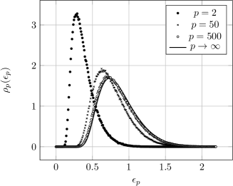
| (21) |
In figure 3 we plotted for different values of : observe that approaches the Kolmogorov distribution in the large limit.
Finally, observe also that the variance of
| (22) |
increases with and that
| (23) |
From a numerical point of view, this means that a computation of requires a larger amount of iterations as increases and fluctuations around the mean value become extremely large in the limit. On the other hand, fluctuations of the optimal cost around its mean value for remain finite
| (24) |
This fact allows to perform a precise computation of for large .
III Optimal cost and correlation function on the circumference
Let us now consider the case of periodic boundary conditions. As discussed in Ref. (Boniolo et al., 2014), the solution for both the cost and the cost , with , is again ordered; however, in this case the mapping is for a certain . In the continuum limit, the solution is a generalised Brownian bridge, , , for a certain constant depending on . The constant can be found by optimality condition on the cost functional (2):
| (25) |
The previous equation can be solved only for and . For , ; therefore, and
| (26) |
For , and therefore the optimality condition becomes
| (27) |
Indeed, we have that
| (28) |
from which the eq. (27) is derived. We have therefore, for ,
| (29) |
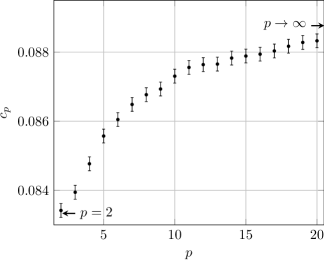


The correlation function can be directly found using the known joint distributions for the Brownian bridge and its sup, eq. (73), and for the sup and inf of a Brownian bridge, eq. (72). After some calculations we obtain
| (30) |
where . The value is very close to the value obtained for , . In figure 5 we plot the values of as function of . Note, finally, that due to the fact that we have imposed pbc, holds in all the previous formulas.
Let us now introduce the normalised transport field
| (31) |
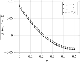
The correlation function can be computed from the covariance matrix observing that the process is still Gaussian. The correlation function is found in the form
| (32) |
where for and .
The optimal cost in the limit can be evaluated as the average spread of the Brownian bridge. Denoting
| (33) |
the distribution of the spread is given by (Dudley, 2002)
| (34) |
where
| (35) |
is the third Jacobi theta function. From eq. (34) the distribution of the optimal cost in the limit is easily derived. Moreover,
| (36) |
with corresponding variance
| (37) |
IV General solution: a continuum approach
In the present section we will justify and generalise the previous results looking at a continuum version of the problem, the so called Monge–Kantorovič problem.
Let us consider the interval , and let us suppose also that two different measures are given on , i.e., the uniform (Lebesgue) measure
| (38) |
and a non uniform measure with measure density ,
| (39) |
We ask for the optimal map such that the following transport condition is satisfied
| (40) |
and minimises the following functional
| (41) |
It can be proved (Villani, 2008) that for eq. (40) can be rewritten as a change-of-variable formula:
| (42) |
We will restrict therefore to the case . Imposing pbc, that is , the solution of (42) determines the optimal map up to a constant as
| (43) |
In the previous equation we have introduced
| (44) |
Note that . The value of must be determined requiring that the functional (41) is minimum: we have that
| (45) |
If instead obc are considered, then and the solution is obtained explicitly .
Let us now suppose that and that the measure is obtained as a limit measure of a random atomic measure of the form
| (46) |
where is a set of points uniformly randomly distributed in . The previous measure can be written as
| (47) |
where we have introduced
| (48) |
Observe now that is a sum of independent identically distributed random variables. From the central limit theorem, we have that is normally distributed as
| (49) |
Remarkably the previous distribution does not depend on . Moreover, the and are independent random variables for , being Gaussian distributed and , where the average is intended over the possible values . In eq. (47) the Karhunen–Loève expansion for the Brownian bridge (Barczy and Iglói, 2010) on the interval appears:
| (50) |
It follows that can be written for large , up to irrelevant additive constants, as
| (51) |
and therefore we cannot associate a density measure to it, due to the fact that is not differentiable.
However the solution of the matching problem in the continuum can be still obtained directly from eq. (39); considering pbc, then
| (52) |
Denoting by
| (53) |
it follows that
| (54) |
where is a constant depending on and . Adopting the notation
| (55) |
for two positive real functions and depending on , note that
| (56) |
for some positive constant depending on . Indeed, in the discrete case, from the fact that the solution must be ordered, in the large limit it can be easily seen that
| (57) |
where is the cost functional (41) in which the measure (46) is adopted. Therefore, . Moreover, note also that . For , eq. (45) becomes
| (58) |
where the first integral is intended in the Stratonovič sense. The result is in agreement with the one presented in Section III. If we consider the transport cost functional
| (59) |
the matching problem has the same solution obtained for the cost (41) for all finite values of , , due to the fact that the function is monotone. However, for the functional cost (59), in the limit, we can reproduce the computations of Section III, obtaining
| (60) |
If obc are considered, then and we have simply, ,
| (61) |
It can be easily seen that
| (62) |
where .
V Conclusions
In the present work we solved the Euclidean bipartite matching problem on the interval , using the cost functional (2) in the continuum limit, , for , both with open boundary conditions and with periodic boundary conditions. The solution is based on the exact correspondence between the optimal map and a Brownian bridge process on the same interval. Moreover, we computed the correlation function for the optimal map and we observed that in all considered cases it has the form
| (63) |
for some constant depending on the adopted boundary conditions and on the value for the optimal cost. Note that if we consider the problem of a matching of random -points to lattice -points on the interval , for the correlation function assumes the form
| (64) |
where is the signed distance between and its corresponding inverse image under the action of the optimal map. It follows that for the correlation function has a divergent part, , depending through on the specific details of the problem (e.g., the boundary conditions adopted or the value of ), a universal finite part and a (universal) finite size correction . We obtained also numerical evidences of the validity of eq. (64) for different values of both with obc and with pbc: an exact derivation of for obc and for and for pbc was presented. This fact suggests that all Euclidean matching problems in one dimension with strictly convex cost functionals belong to the same universality class and that the specific details of the model determine only the value of the constant in the divergent contribution . Similarly, on the interval eq. (32) becomes
| (65) |
in which the universal part is given by the constant and finite size corrections scale as up to a scaling factor depending on .
VI Acknowledgements
The authors are grateful to Luigi Ambrosio, from Scuola Normale Superiore in Pisa, and Andrea Sportiello, from Université Paris 13, for useful and stimulating discussions.
Appendix A Joint distribution for the solution of the problem with open boundary conditions
In the present section we derive the joint distribution of the matching map for the solution of the Euclidean bipartite matching problem on the line. In the hypothesis that , , let us consider -points , , and evaluate the following quantity:
| (66) |
where , , , and
| (67) |
Note that the previous equation has the form of a multinomial distribution. Introducing the rescaled variable , in the large limit we obtain a multivariate Gaussian distribution in the variable , , , whose covariance matrix is given by the degenerate matrix
| (68) |
Note that : the constraint reduces the rank of the matrix from to (we have indeed independent variables). In this case, no density distribution exists in the -dimensional space of variables , due to the fact that an additional constraint, , holds, and therefore the distribution is singular. We need to restrict therefore to the subspace of variables . The distribution is still a multivariate Gaussian but with covariance matrix with . The covariance matrix is positive definite and non singular on this subspace, being and
| (69) |
The joint distribution is therefore
| (70) |
The previous distribution is exactly the joint distribution for the Brownian bridge process, proving the equivalence of the processes in the large limit. In particular, the two point joint distribution for the Brownian bridge is given by eq. (70) for :
| (71) |
where is assumed.
Appendix B Probability distributions for the Brownian bridge
In the present section we briefly present, without proofs, some fundamental probability results on the Brownian bridge process and on some noteworthy probability distributions related to it. As explained before, the distribution for the sup of the absolute value of a Brownian bridge is given by the well known Kolmogorov distribution, eq. (20). Using the reflection principle and Bayes’ theorems, it can be also proved that (Beghin and Orsingher, 1999; Dudley, 2002)
| (72) |
For and , it can be easily obtained that
| (73) |
The computation of (36) can be easily performed using the distribution of the sup of the Brownian bridge
| (74) |
References
- Kuhn (1955) H. W. Kuhn, Naval research logistics quarterly 2, 83 (1955).
- Munkres (1957) J. Munkres, Journal of the Society for Industrial and Applied Mathematics 5, pp. 32 (1957), ISSN 03684245.
- Edmonds and Karp (1972) J. Edmonds and R. M. Karp, Journal of the ACM 19, 248 (1972).
- Aldous (2001) D. J. Aldous, Random Structures and Algorithms pp. 381–418 (2001).
- Mézard and Parisi (1985) M. Mézard and G. Parisi, Journal de Physique Lettres 46, 771 (1985).
- Mézard and Parisi (1988) M. Mézard and G. Parisi, Journal de Physique 49, 2019 (1988).
- Boniolo et al. (2014) E. Boniolo, S. Caracciolo, and A. Sportiello, arXiv (2014), eprint arXiv:1403.1836v1.
- Caracciolo et al. (2014) S. Caracciolo, C. Lucibello, G. Parisi, and G. Sicuro, Physical Review E (2014), to appear.
- Leighton and Shor (1989) T. Leighton and P. W. Shor, Combinatorica 9, 161 (1989).
- Shor and Yukich (1991) P. W. Shor and J. E. Yukich, The Annals of Probability 19, 1338 (1991).
- Shepp (1982) L. A. Shepp, The Annals of Probability 10, 234 (1982).
- Dudley (2002) R. Dudley, Real Analysis and Probability, Cambridge Studies in Advanced Mathematics (Cambridge University Press, 2002).
- Villani (2008) C. Villani, Optimal Transport: Old and New, Grundlehren der mathematischen Wissenschaften (Springer, 2008), ISBN 9783540710509.
- Barczy and Iglói (2010) M. Barczy and E. Iglói, Central European Journal of Mathematics 9, 65 (2010).
- Beghin and Orsingher (1999) L. Beghin and E. Orsingher, Lithuanian Mathematical Journal 39, 157 (1999).