Asymptotic Laplacian-Energy-Like Invariant of Lattices

Abstract

Let $\mu_{1}\geq\mu_{2}\geq\cdots\geq\mu_{n}$ denote the Laplacian eigenvalues of $G$ with $n$ vertices. The Laplacian-energy-like invariant, denoted by $LEL(G)=\sum_{i=1}^{n-1}\sqrt{\mu_{i}}$, is a novel topological index. In this paper, we show that the Laplacian-energy-like per vertex of various lattices is independent of the toroidal, cylindrical, and free boundary conditions. Simultaneously, the explicit asymptotic values of the Laplacian-energy-like in these lattices are obtained. Moreover, our approach implies that in general the Laplacian-energy-like per vertex of other lattices is independent of the boundary conditions.

Keywords: Lattice;     Laplacian-energy-like invariant;    Laplacian spectrum

1 Introduction

Throughout this paper we concerned with finite undirected connected simple graphs. Let $G$ be a graph with vertices labelled $1,2,\dots,n$. The adjacency matrix $A(G)$ of $G$ is an $n\times n$ matrix with the $(i,j)$-entry equal to 1 if vertices $i$ and $j$ are adjacent and 0 otherwise. Supposed $D(G)=diag(d_{1}(G),d_{2}(G),\ldots,d_{n}(G))$ be the degree diagonal matrix of $G$, where $d_{i}(G)$ is the degree of the vertex $i$, $i=1,2,\ldots,n$. Let $L(G)=D(G)-A(G)$ is called the Laplacian matrix of $G$. Then, the eigenvalues of $A(G)$ and $L(G)$ are called eigenvalues and Laplacian eigenvalues of $G$, denoted by $\lambda_{1},\lambda_{2},\dots,\lambda_{n}$ and $\mu_{1},\mu_{2},\dots,\mu_{n}$, respectively. The underlying graph theoretical definitions and notations follow [5].

Gutman has defined the energy of a graph $G$ with $n$ vertices [2], denoted by $E(G)$, as

$$E(G)=\sum_{i=1}^{n}|\lambda_{i}|.$$

Let $G$ be a graph of order $n$ with Laplacian spectrum $\mu_{1}\geq\mu_{2}\geq\cdots\geq\mu_{n}.$ The Laplacian-energy-like invariant of G, LEL for short, is defined as

$$LEL(G)=\sum_{i=1}^{n-1}\sqrt{\mu_{i}}.$$

The concept of $LEL(G)$ was introduced by J. Liu and B. Liu ([11], 2008), where it was shown that it has similar features as graph energy.

Gutman et al. pointed out in [4] that $LEL(G)$ is more similar to $E(G)$ than to $LE(G)$. The Laplacian-energy-like invariant describes well the properties which are accounted by the majority of molecular descriptors: motor octane number, entropy, molar volume, molar refraction, particularly the acentric factor AF parameter, but also more difficult properties like boiling point, melting point and partition coefficient Log P. [9, 13]. D. Stevanovi$\acute{c}$ et al. [13] have proved that $LEL(G)$ has the properties as good as the Randi$\acute{c}$ $\chi$ index and better than the Wiener index which is a distance based index. Besides, it is well defined mathematically and shows interesting relationships in particular classes of graphs, these recommending $LEL(G)$ as a noval and powerful topological index.

The index has attracted extensive attention due to its wide applications in physics, chemistry, graph theory, etc. [3, 12, 17]. Details on its theory can be found in the survey on the Laplacian-energy-like invariant [9], the recent papers [15, 16], and the references cited therein. Due to its structure, lattices are of special interest, especially the chemical and physical indices of some lattices were studied extensively, see for instance [10, 18, 25].

One of reasons we investigated $LEL(G)$ of lattices is that some physical and chemical indices of lattices have been presented in [10, 25, 26], however, there is seldom results on $LEL(G)$ of lattices. Another reason is, there are a great deal of analogies between the properties of $E(G)$ and $LEL(G)$, asymptotic energy of lattices has investigated in chemical physics[1, 23], it is natural for us to consider asymptotic $LEL(G)$ of various lattices.

The energy $E(G)$ of toroidal lattices have been studied in [1], the Kirchhoff index of some toroidal lattices has also investigated in [10], a very elementary and natural question is that if $G$ are lattices, how about $LEL(G)$? It is an interesting problem to study the Laplacian-energy-like of some lattices with various boundary condition. Motivated by results above, we consider the problem of computation of the $LEL(G)$ of some lattices in this article.

The rest of the paper is organized as follows. In Section 2, we propose the asymptotic Laplacian-energy-like of square lattices and give the related explanations. We provide a detailed derivation of the asymptotic Laplacian-energy-like change due to edge deletion in Section 3. The asymptotic Laplacian-energy-like of hexagonal, triangular, and $3^{3}4^{2}$ lattices with three boundary conditions are investigated in Section 4. We present concluding remarks and conclude the paper in Section 5.

2 Asymptotic Laplacian-energy-like of square lattices

Given graphs $G$ and $H$ with vertex sets $U$ and $V$, the cartesian product $G\Box H$ of graphs $G$ and $H$ is a graph such that the vertex set of $G\Box H$ is the cartesian product $U\Box V$; and any two vertices $(u,u^{\prime})$ and $(v,v^{\prime})$ are adjacent in $G\Box H$ if and only if either $u=v$ and $u^{\prime}$ is adjacent with $v^{\prime}$ in $H$, or $u^{\prime}=v^{\prime}$ and $u$ is adjacent with $v$ in $G$ [5].

Let $P_{m}\Box P_{n}$, $P_{m}\Box C_{n}$, and $C_{m}\Box C_{n}$, denote the square lattices with free, cylindrical and toroidal boundary conditions, respectively, where $P_{n}$ and $C_{n}$ denote the path and the cycle with $n$ vertices. Obviously, $P_{m}\Box P_{n}$ is a sequence of spanning subgraphs of the sequence $P_{m}\Box C_{n}$ of finite graphs, and $P_{m}\Box C_{n}$ is a sequence of spanning subgraphs of the sequence $C_{m}\Box C_{n}$ of finite graphs. Particularly,

$$\lim_{m,n\to\infty}\frac{\left|\{v\in V(P_{m}\Box P_{n}):~{}d_{P_{m}\Box P_{n}}(v)=d_{C_{m}\Box C_{n}}(v)\}\right|}{\mid V(C_{m}\Box C_{n})\mid}$$

$$=\lim_{m,n\to\infty}\frac{\left|\{v\in V(P_{m}\Box C_{n}):~{}d_{P_{m}\Box C_{n}}(v)=d_{C_{m}\Box C_{n}}(v)\}\right|}{\mid V(C_{m}\Box C_{n})\mid}=1,$$

that is, almost all vertices of $C_{m}\Box C_{n}$ and $P_{m}\Box C_{n}$ (resp. $C_{m}\Box C_{n}$ and $P_{m}\Box P_{n}$) have the same degrees. Let $G_{1},G_{2}$ be graphs with adjacency matrices $A_{1},$ $A_{2}$, degree matrices $D_{1},$ $D_{2}$ and Laplacan matrices $L_{1},$ $L_{2},$ respectively. Then $L_{1}=D_{1}-A_{1},L_{2}=D_{2}-A_{2}.$ If $\mu_{i}(G_{1}),\mu_{j}(G_{2})$ are Laplacian eigenvalues of $G_{1},G_{2}$, then the Laplacian eigenvalues of $G_{1}\Box G_{2}$ are all possible sums $\mu_{i}(G_{1})+\mu_{j}(G_{2})$, as noted in [14]. On the other hand, it is well known that the Laplacian eigenvalues of a path $P_{m}$ and a cycle $C_{m}$ are $2-2cos\frac{i\pi}{n}(i=0,1,\dots,n-1)$ and $2-2cos\frac{2\pi j}{n}(j=0,1,\dots,m-1)$ [14], respectively. Consequently, the Laplacian eigenvalues of $P_{m}\Box P_{n}$ (resp. $P_{m}\Box C_{n}$ and $C_{m}\Box C_{n}$) are $4-2cos\frac{i\pi}{m}-2cos\frac{j\pi}{n},i=0,1,\dots,n-1;j=0,1,\dots,m-1$ (resp. $4-2cos\frac{i\pi}{m}-2cos\frac{2j\pi}{n},i=0,1,\dots,n-1;j=0,1,\dots,m-1$ and $4-2cos\frac{2i\pi}{m}-2cos\frac{2j\pi}{n},i=0,1,\dots,n-1;j=0,1,\dots,m-1$).

Therefore, the Laplacian-energy-like per vertex of $P_{m}\Box P_{n}$, $P_{m}\Box C_{n}$, and $C_{m}\Box C_{n}$ are defined as

$$1.\ \lim_{m\to\infty}\lim_{n\to\infty}\frac{LEL\Big{(}P_{m}\Box P_{n}\Big{)}}{\mid V(P_{m}\Box P_{n})\mid}=\lim_{m\to\infty}\lim_{n\to\infty}\frac{1}{mn}\sum_{i=0}^{m-1}\sum_{j=0}^{n-1}\sqrt{4-2cos\frac{i\pi}{m}-2cos\frac{j\pi}{n}}$$

$$=\int_{0}^{1}\int_{0}^{1}\sqrt{4-2cos\pi x-2cos\pi y}\ ~{}dxdy=\frac{1}{\pi^{2}}\int_{0}^{\pi}\int_{0}^{\pi}\sqrt{4-2cosx-2cosy}\ ~{}dxdy\approx 1.9162.$$

$$2.\ \lim_{m\to\infty}\lim_{n\to\infty}\frac{LEL\Big{(}P_{m}\Box C_{n}\Big{)}}{\mid V(P_{m}\Box C_{n})\mid}=\lim_{m\to\infty}\lim_{n\to\infty}\frac{1}{mn}\sum_{i=0}^{m-1}\sum_{j=0}^{n-1}\sqrt{4-2cos\frac{i\pi}{m}-2cos\frac{2j\pi}{n}}$$

$$=\int_{0}^{1}\int_{0}^{1}\sqrt{4-2cos\pi x-2cos2\pi y}\ ~{}dxdy=\frac{1}{2\pi^{2}}\int_{0}^{\pi}\int_{0}^{2\pi}\sqrt{4-2cosx-2cosy}\ ~{}dxdy\approx 1.9162.$$

$$3.\ \lim_{m\to\infty}\lim_{n\to\infty}\frac{LEL\Big{(}C_{m}\Box C_{n}\Big{)}}{\mid V(C_{m}\Box C_{n})\mid}=\lim_{m\to\infty}\lim_{n\to\infty}\frac{1}{mn}\sum_{i=0}^{m-1}\sum_{j=0}^{n-1}\sqrt{4-2cos\frac{2i\pi}{m}-2cos\frac{2j\pi}{n}}$$

$$=\int_{0}^{1}\int_{0}^{1}\sqrt{4-2cos2\pi x-2cos2\pi y}\ ~{}dxdy=\frac{1}{4\pi^{2}}\int_{0}^{2\pi}\int_{0}^{2\pi}\sqrt{4-2cosx-2cosy}\ ~{}dxdy\approx 1.9162.$$

The numerical integration value in last line is calculated with software MATLAB calculation.

Remark 2.1 By using computer software MATLAB, we can easily get that the above numerical integration values, which imply that $P_{m}\Box P_{n}$, $P_{m}\Box C_{n}$ and $C_{m}\Box C_{n}$ have the same asymptotic Laplacian-energy-like $LEL(P_{m}\Box P_{n})=LEL(P_{m}\Box C_{n})=LEL(C_{m}\Box C_{n})\approx 1.9162mn$ as $m,n$ approach infinity.

Remark 2.2 The asymptotic Laplacian-energy-like $LEL(G)$ of square lattices is independent on the three boundary conditions, i.e., the free, cylindrical and toroidal boundary conditions.

The phenomenon above is not accidental, the related explanations are proposed in next section. Our method implies that in general the Laplacian-energy-like per vertex of lattices is independent of the boundary conditions.

3 Graph asymptotic Laplacian-energy-like change due to edge deletion

We propose a detailed derivation of the asymptotic Laplacian-energy-like change due to edge deletion, in our proof, some techniques in [1] are referred to. Recall some results which will be used in our discussion. The authors [11] verified the following theorem.

Theorem 3.1

([11]) Let $G$ be a graph on $n$ vertices with $m$ edges, then

$$\sqrt{2m}\leq LEL(G)\leq\sqrt{2}m.$$

The first equality is attained if and only if $G\cong\overline{K_{n}}$ or $K_{2}\cup(n-2)K_{1},$ and the second equality is attained if and only if $G\cong rK_{2}\cup(n-2r)K_{1}$, where $0\leq r\leq\lfloor\frac{n}{2}\rfloor.$

According to Theorem 3.1, one can easily get that

Lemma 3.2

Let $G$ be a graph on $n$ vertices with $m$ edges, then

$$LEL(G)\leq\sqrt{2}m<2m.$$

The authors [6, 7] investigated how the energy of a graph changes when edges are removed, and obtained the following consequence.

Lemma 3.3

([6, 7]) Let $H$ be an induced subgraph of a graph $G.$ Then

$$E(G)-E(H)\leq E(G-E(H))\leq E(G)+E(H).$$

In addition, the authors [1] obtained that

$$\mid E(G)-E(H)\mid\leq E(G-E(H))\leq E(G)+E(H).$$

With a similar method, one can prove the following result.

Lemma 3.4

Let $H$ be a subgraph of a graph $G.$ Then

$$\mid LEL(G)-LEL(H)\mid\leq LEL(G-E(H))\leq LEL(G)+LEL(H).$$

Consider two graphs $G$ and $H$ $(V(G)\cap V(H)$ may be disjoint), denoted by

$$\Delta(G,H)=\mid E(G)\mid+\mid E(H)\mid-2\mid E(G)\cap E(H)\mid,$$

i.e., $\Delta(G,H)$ equals the number of edges of symmetric difference of $E(G)$ and $E(H)$.

Theorem 3.5

Let $\{G_{n}\}$ and $\{H_{n}\}$ be two sequences of graphs such that

$$\lim_{n\to\infty}\frac{\Delta(G_{n},H_{n})}{LEL(G_{n})}=0.$$

Then

$$\lim_{n\to\infty}\frac{LEL(H_{n})}{LEL(G_{n})}=1.$$

Proof. Let $F_{n}$ be the subgraph of $G_{n}$ or $H_{n}$ induced by $E(G)\cap E(H).$ Note that

$$\left|\frac{LEL(H_{n})}{LEL(G_{n})}-1\right| =\left|\frac{LEL(H_{n})-LEL(G_{n})}{LEL(G_{n})}\right|=\left|\frac{LEL(H_{n})-LEL(F_{n})+LEL(F_{n})-LEL(G_{n})}{LEL(G_{n})}\right|$$

$$\leq\left|\frac{LEL(G_{n})-LEL(F_{n})}{LEL(G_{n})}\right|+\left|\frac{LEL(H_{n})-LEL(F_{n})}{LEL(G_{n})}\right|.$$

By Lemma 3.2 and Lemma 3.4,

$$\mid LEL(G_{n})-LEL(F_{n})\mid\leq LEL(G_{n}-E(F_{n}))\leq 2\left|E(G_{n})\right|-2\left|E(F_{n})\right|,$$

$$\mid LEL(H_{n})-LEL(F_{n})\mid\leq LEL(H_{n}-E(F_{n}))\leq 2\left|E(H_{n})\right|-2\left|E(F_{n})\right|.$$

Consequently,

$$\left|\frac{LEL(H_{n})}{LEL(G_{n})}-1\right|\leq\frac{2\Big{(}\mid E(G_{n})\mid+\mid E(H_{n})\mid-2\mid E(F_{n})\mid\Big{)}}{LEL(G_{n})}=\frac{2\Delta(G_{n},H_{n})}{LEL(G_{n})},$$

implying the theorem holds. $\blacksquare$

Based on Theorem 3.5, one can straightforwardly arrive to that

Theorem 3.6

Let $\{G_{n}\}$ be a sequence of finite simple graphs with bounded average degree such that

$$\lim_{n\to\infty}\left|V(G_{n})\right|=\infty,\lim_{n\to\infty}\frac{LEL(G_{n})}{\left|V(G_{n})\right|}=h\neq 0.$$

Let $\{H_{n}\}$ be a sequence of spanning subgraphs of $\{G_{n}\}$ such that

$$\lim_{n\to\infty}\frac{\left|v\in V(H_{n}):d_{H_{n}(v)}=d_{G_{n}(v)}\right|}{\left|V(G_{n})\right|}=1,$$

then

$$\lim_{n\to\infty}\frac{LEL(H_{n})}{\left|V(G_{n})\right|}=h.$$

That is, $G_{n}$ and $H_{n}$ have the same asymptotic Laplacian-energy-like.

A direct sequence of Theorem 3.6 is that $P_{n}\square P_{n}$,$P_{n}\square C_{n}$, and $C_{n}\square C_{n}$ have the same asymptotic Laplacian-energy-like which is shown in the introduction. More generally, by Theorem 3.6, we have

Remark 3.7 Let $G_{i}=P_{n}$ or $G_{i}=C_{n}$, $i=1,2,\dots,k,$ and $k$ be a constant. If $n$ is sufficiently large, then the asymptotic Laplacian-energy-like of the $n$-dimensional lattices

$$LEL(G_{1}\square G_{2}\square\dots\square G_{k})\approx\frac{n^{k}}{\pi^{k}}\int_{0}^{\pi}\int_{0}^{\pi}\dots\int_{0}^{\pi}\sqrt{\sum_{i=1}^{k}\Big{(}2-2cosx_{i}\Big{)}}~{}dx_{1}~{}dx_{2}\dots dx_{k}.$$

Remark 3.8  Theorem 3.6 provides a very effective approach to handle the asymptotic Laplacian-energy-like of a graph with bounded average degree.

We will use the approach above to deal with the asymptotic Laplacian-energy-like of some lattices in the next subsections.

4 Asymptotic Laplacian-energy-like of some lattices

4.1 The hexagonal lattice

Our notation for the hexagonal lattices follows [1, 24]. The hexagonal lattices with toroidal, cylindrical and free boundary conditions, denoted by $H^{t}(m,n)$, $H^{c}(m,n)$, and $H^{f}(m,n)$ are illustrated in Figure 1, respectively, where $(a_{1},b_{1}),(a_{2},b_{2}),\dots,(a_{m+1},b_{m+1}),(a_{1},c_{1}^{*}),(c_{1},c_{2}^{*}),(c_{2},c_{3}^{*}),\dots,(c_{n-1},c_{n}^{*}),\\ (c_{n},b_{m+1})$ are edges in $H^{t}(m,n)$, and $(a_{1},b_{1}),(a_{2},b_{2}),\dots,(a_{m+1},b_{m+1})$ are edges in $H^{c}(m,n)$(see Figure 1(b)). If we delete edges $(a_{1},b_{1}),(a_{2},b_{2}),\dots,(a_{m+1},b_{m+1})$ from $H^{c}(m,n)$, then the hexagonal lattice, denoted by $H^{f}(m,n)$, with free boundary condition is obtained (see Figure 1(c)).

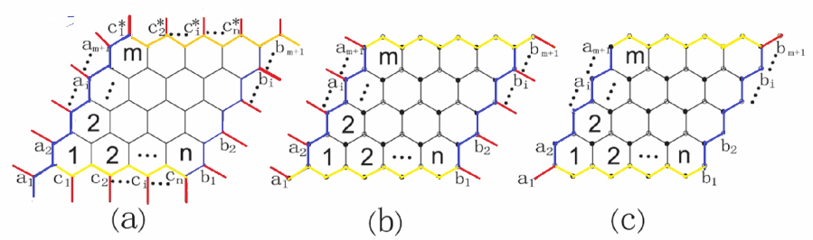
Figure 1: (a) The hexagonal lattice $H^{t}(m,n)$ with toroidal boundary condition; (b) the hexagonal lattice $H^{c}(m,n)$ with cylindrical boundary condition; (c) the hexagonal lattice $H^{f}(m,n)$ with free boundary condition.

A recent approach to compute the Laplacian eigenvalues of $H^{t}(m,n)$ can be found in [3, 18, 19]. Using Equation (6.2.2) in [24], the Laplacian matrix $L(H^{t}(m,n))$ of $H^{t}(m,n)$ is similar to the block diagonal matrix whose diagonal blocks are

$$B_{ij}=\left(\begin{array}[]{cc}3&-1-\omega_{n+1}^{-i}-\omega_{m+1}^{j}\\ -1-\omega_{n+1}^{i}-\omega_{m+1}^{-j}&3\\ \end{array}\right)$$

where $\omega_{s}=cos\frac{2\pi}{s}+isin\frac{2\pi}{s},i=0,1,\dots,m;j=0,1,\dots,n.$ Hence the Laplacian eigenvalues of $H^{t}(m,n)$ are

$$3\pm\sqrt{3+2cos\frac{2\pi i}{m+1}+2cos\frac{2\pi j}{n+1}+2cos\Big{(}\frac{2\pi i}{m+1}+\frac{2\pi j}{n+1}\Big{)}},\ \ i=0,1,\dots,m;j=0,1,\dots,n.$$

By the definition of the Laplacian-energy-like, it is not difficult to prove the following result:

Theorem 4.1

For the hexagonal lattices $H^{t}(m,n),H^{c}(m,n)$ and $H^{f}(m,n)$ with toroidal, cylindrical, and free boundary conditions. Then

$$1.~{}~{}\lim_{m\to\infty}\lim_{n\to\infty}\frac{LEL\Big{(}H^{t}(m,n)\Big{)}}{2(m+1)(n+1)}=\lim_{m\to\infty}\lim_{n\to\infty}\frac{LEL\Big{(}H^{c}(m,n)\Big{)}}{2(m+1)(n+1)}=\lim_{m\to\infty}\lim_{n\to\infty}\frac{LEL\Big{(}H^{f}(m,n)\Big{)}}{2(m+1)(n+1)}\approx 1.6437.$$

$2.~{}LEL\Big{(}H^{t}(m,n)\Big{)}=LEL\Big{(}H^{c}(m,n)\Big{)}=LEL\Big{(}H^{f}(m,n)\Big{)}\approx 3.2714(m+1)(n+1).$

Proof. By definitions of $H^{t}(m,n),H^{c}(m,n)$ and $H^{f}(m,n)$, it is obvious that $H^{c}(m,n)$ and $H^{f}(m,n)$ are spanning subgraphs of $H^{t}(m,n)$. Furthermore, the degree of almost all vertices of $H^{t}(m,n),H^{c}(m,n)$ and $H^{f}(m,n)$ are 3. Hence, by Theorem 3.6, one can obtian that

$$\lim_{m\to\infty}\lim_{n\to\infty}\frac{LEL\Big{(}H^{t}(m,n)\Big{)}}{2(m+1)(n+1)}=\lim_{m\to\infty}\lim_{n\to\infty}\frac{LEL\Big{(}H^{c}(m,n)\Big{)}}{2(m+1)(n+1)}=\lim_{m\to\infty}\lim_{n\to\infty}\frac{LEL\Big{(}H^{f}(m,n)\Big{)}}{2(m+1)(n+1)}.$$

It suffices to prove that

$$\lim_{m\to\infty}\lim_{n\to\infty}\frac{LEL\Big{(}H^{t}(m,n)\Big{)}}{2(m+1)(n+1)}$$

$$= \lim_{m\to\infty}\lim_{n\to\infty}\frac{1}{2(m+1)(n+1)}\sum_{i=0}^{m}\sum_{j=0}^{n}\sqrt{3+\sqrt{3+2cos\alpha_{i}+2cos\beta_{j}+2cos(\alpha_{i}+\beta_{j})}}$$

$$+\lim_{m\to\infty}\lim_{n\to\infty}\frac{1}{2(m+1)(n+1)}\sum_{i=0}^{m}\sum_{j=0}^{n}\sqrt{3-\sqrt{3+2cos\alpha_{i}+2cos\beta_{j}+2cos(\alpha_{i}+\beta_{j})}}$$

$$= \frac{1}{2}\int_{0}^{1}\int_{0}^{1}\sqrt{3+\sqrt{3+2cos2\pi x+2cos2\pi y+2cos2\pi(x+y)}}\ ~{}dxdy$$

$$+\frac{1}{2}\int_{0}^{1}\int_{0}^{1}\sqrt{3-\sqrt{3+2cos2\pi x+2cos2\pi y+2cos2\pi(x+y)}}\ ~{}dxdy$$

$$= \frac{1}{8\pi^{2}}\int_{0}^{2\pi}\int_{0}^{2\pi}\sqrt{3+\sqrt{3+2cosx+2cosy+2cos(x+y)}}\ ~{}dxdy$$

$$+\frac{1}{8\pi^{2}}\int_{0}^{2\pi}\int_{0}^{2\pi}\sqrt{3-\sqrt{3+2cosx+2cosy+2cos(x+y)}}\ ~{}dxdy$$

$$\approx 1.6437.$$

The above numerical integration value implies that the hexagonal lattices $H^{t}(m,n),H^{c}(m,n)$ and $H^{f}(m,n)$ with toroidal, cylindrical, and free boundary conditions have the same asymptotic Laplacian-energy-like, i.e., $LEL\Big{(}H^{t}(m,n)\Big{)}=LEL\Big{(}H^{c}(m,n)\Big{)}=LEL\Big{(}H^{f}(m,n)\Big{)}\approx 3.2714(m+1)(n+1)$ as $m,n$ tends to infinity. $\blacksquare$

4.2 The 3.12.12 lattice

Our notation for the 3.12.12 lattices follows [12, 25]. The 3.12.12 lattice with toroidal boundary condition, denoted by $J^{t}(m,n)$, is the graph illustrated in Figure 2(a).

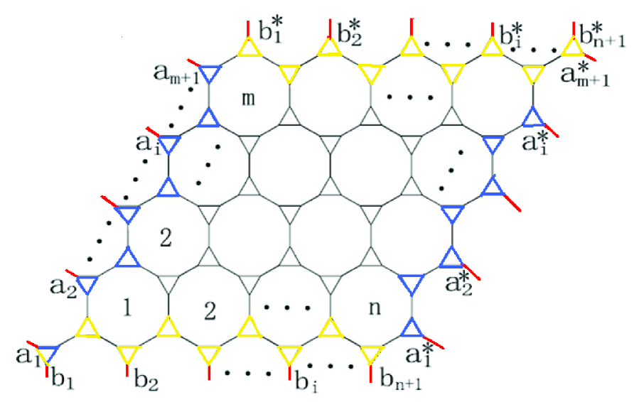
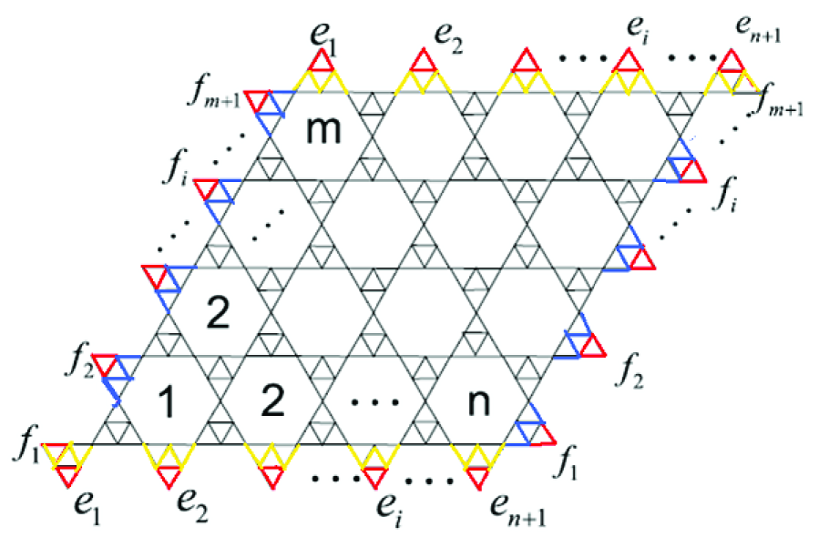
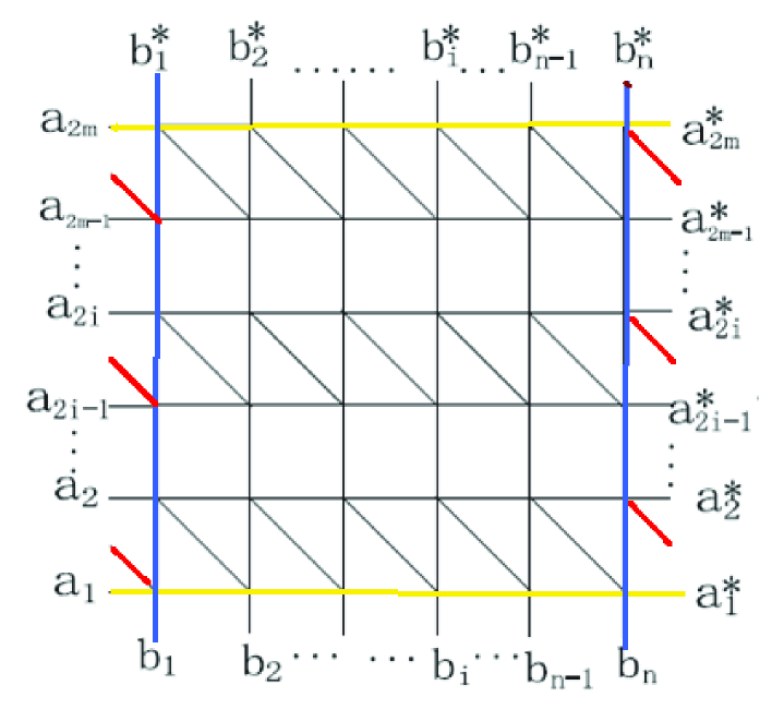
Figure 2: (a) The 3-12-12 lattice with toroidal boundary condition; (b) The triangular kagom$\acute{e}$ lattice with toroidal boundary condition; (c) the $3^{3}.4^{2}$ lattice with toroidal boundary condition.

Recently, the adjacency spectrum of 3.12.12 lattice has been proposed in [12].

Theorem 4.2

[12] Let $J^{t}(m,n)$ be the 3.12.12 lattice with toroidal boundary condition. Then the adjacency spectrum is

$$Spec_{A}(J^{t}(m,n)) = \textbf{\{}\underbrace{-2,-2,\dots,-2}_{(m+1)(n+1)},\underbrace{0,0,\dots,0}_{(m+1)(n+1)}\textbf{\}}$$

$$\bigcup\left\{\frac{1\pm\sqrt{13\pm 4\sqrt{3+2cos\alpha_{i}+2cos\beta_{j}+2cos\Big{(}\alpha_{i}+\beta_{j}\Big{)}}}}{2}:0\leq i\leq m,0\leq j\leq n\right\},$$

where $\alpha_{i}=\frac{2\pi i}{m+1},\beta_{j}=\frac{2\pi j}{n+1},i=0,1,\dots,m;j=0,1,\dots,n.$

The following result has been obtained in [22], which is an important relationship between $Spec_{A}(G)$ and $Spec_{L}(G)$. Suppose that $G$ is an $r$-regular graph with $n$ vertices and $Spec_{A}(G)=\{\lambda_{1},\lambda_{2},\dots,\lambda_{n}\}.$ Then

$$Spec_{L}(G)=\Big{\{}r-\lambda_{1},r-\lambda_{2},\dots,r-\lambda_{n}\Big{\}}.$$

Note that $J^{t}(m,n)$ is the line graph of the subdivision of $H^{t}(m,n)$ which is a $3$-regular graph with $2(m+1)(n+1)$ vertices and $J^{t}(m,n)$ has $6(m+1)(n+1)$ vertices. Hence, we arrive to that

Theorem 4.3

Let $J^{t}(m,n)$ be the 3.12.12 lattice with toroidal boundary condition. Then the Laplacian spectrum is

$$Spec_{L}(J^{t}(m,n)) = \textbf{\{}\underbrace{5,5,\dots,5}_{(m+1)(n+1)},\underbrace{3,3,\dots,3}_{(m+1)(n+1)}\textbf{\}}$$

$$\bigcup\left\{\frac{5\pm\sqrt{13\pm 4\sqrt{3+2cos\alpha_{i}+2cos\beta_{j}+2cos\Big{(}\alpha_{i}+\beta_{j}\Big{)}}}}{2}:0\leq i\leq m,0\leq j\leq n\right\},$$

where $\alpha_{i}=\frac{2\pi i}{m+1},\beta_{j}=\frac{2\pi j}{n+1},i=0,1,\dots,m;j=0,1,\dots,n.$

By the definition of the Laplacian-energy-like $LEL(G)$, one can easily arrive to the following theorem.

Theorem 4.4

For $J^{t}(m,n),J^{c}(m,n)$ and $J^{f}(m,n)$ with toroidal, cylindrical, and free boundary conditions. Then

$$1.~{}~{}\lim_{m\to\infty}\lim_{n\to\infty}\frac{LEL\Big{(}J^{t}(m,n)\Big{)}}{6(m+1)(n+1)}=\lim_{m\to\infty}\lim_{n\to\infty}\frac{LEL\Big{(}J^{c}(m,n)\Big{)}}{6(m+1)(n+1)}=\lim_{m\to\infty}\lim_{n\to\infty}\frac{LEL\Big{(}J^{f}(m,n)\Big{)}}{6(m+1)(n+1)}\approx 1.3375.$$

$2.~{}~{}LEL\Big{(}J^{t}(m,n)\Big{)}=LEL\Big{(}J^{c}(m,n)\Big{)}=LEL\Big{(}J^{f}(m,n)\Big{)}\approx 8.0250(m+1)(n+1).$

Proof. By definitions of $H^{t}(m,n),H^{c}(m,n)$ and $H^{f}(m,n)$, one can know that $H^{c}(m,n)$ and $H^{f}(m,n)$ are spanning subgraphs of $H^{t}(m,n)$. Furthermore, the degree of almost all vertices of $H^{t}(m,n),H^{c}(m,n)$ and $H^{f}(m,n)$ are 3. Therefore, by Theorem 3.6 it is not difficult to arrive to that

$$\lim_{m\to\infty}\lim_{n\to\infty}\frac{LEL\Big{(}J^{t}(m,n)\Big{)}}{6(m+1)(n+1)}=\lim_{m\to\infty}\lim_{n\to\infty}\frac{LEL\Big{(}J^{c}(m,n)\Big{)}}{6(m+1)(n+1)}=\lim_{m\to\infty}\lim_{n\to\infty}\frac{LEL\Big{(}J^{f}(m,n)\Big{)}}{6(m+1)(n+1)}.$$

It suffices to prove that

$$\lim_{m\to\infty}\lim_{n\to\infty}\frac{LEL\Big{(}J^{t}(m,n)\Big{)}}{6(m+1)(n+1)}$$

$$= \lim_{m\to\infty}\lim_{n\to\infty}\frac{1}{12(m+1)(n+1)}\sum_{i=0}^{m}\sum_{j=0}^{n}\sqrt{5-\sqrt{13-4\sqrt{3+2cos\alpha_{i}+2cos\beta_{j}+2cos\Big{(}\alpha_{i}+\beta_{j}\Big{)}}}}$$

$$+\lim_{m\to\infty}\lim_{n\to\infty}\frac{1}{12(m+1)(n+1)}\sum_{i=0}^{m}\sum_{j=0}^{n}\sqrt{5-\sqrt{13+4\sqrt{3+2cos\alpha_{i}+2cos\beta_{j}+2cos\Big{(}\alpha_{i}+\beta_{j}\Big{)}}}}$$

$$+\lim_{m\to\infty}\lim_{n\to\infty}\frac{1}{12(m+1)(n+1)}\sum_{i=0}^{m}\sum_{j=0}^{n}\sqrt{5+\sqrt{13-4\sqrt{3+2cos\alpha_{i}+2cos\beta_{j}+2cos\Big{(}\alpha_{i}+\beta_{j}\Big{)}}}}$$

$$+\lim_{m\to\infty}\lim_{n\to\infty}\frac{1}{12(m+1)(n+1)}\sum_{i=0}^{m}\sum_{j=0}^{n}\sqrt{5+\sqrt{13+4\sqrt{3+2cos\alpha_{i}+2cos\beta_{j}+2cos\Big{(}\alpha_{i}+\beta_{j}\Big{)}}}}$$

$$+\frac{\sqrt{3}+\sqrt{5}}{6}$$

$$= \frac{1}{12}\int_{0}^{1}\int_{0}^{1}\sqrt{5-\sqrt{13-4\sqrt{3+2cos2\pi x+2cos2\pi y+2cos2\pi\Big{(}x+y\Big{)}}}}~{}dxdy$$

$$+\frac{1}{12}\int_{0}^{1}\int_{0}^{1}\sqrt{5-\sqrt{13+4\sqrt{3+2cos2\pi x+2cos2\pi y+2cos2\pi\Big{(}x+y\Big{)}}}}~{}dxdy$$

$$+\frac{1}{12}\int_{0}^{1}\int_{0}^{1}\sqrt{5+\sqrt{13-4\sqrt{3+2cos2\pi x+2cos2\pi y+2cos2\pi\Big{(}x+y\Big{)}}}}~{}dxdy$$

$$+\frac{1}{12}\int_{0}^{1}\int_{0}^{1}\sqrt{5+\sqrt{13+4\sqrt{3+2cos2\pi x+2cos2\pi y+2cos2\pi\Big{(}x+y\Big{)}}}}~{}dxdy+\frac{\sqrt{3}+\sqrt{5}}{6}$$

$$\approx 1.3375.$$

The above numerical integration value implies that $J^{t}(m,n),J^{c}(m,n)$ and $J^{f}(m,n)$ have the same asymptotic Laplacian-energy-like, i.e., $LEL\Big{(}J^{t}(m,n)\Big{)}=LEL\Big{(}J^{c}(m,n)\Big{)}=LEL\Big{(}J^{f}(m,n)\Big{)}\\ \approx 8.0250(m+1)(n+1)$ as $m,n$ tends to infinity. $\blacksquare$

4.3 The triangular kagom$\acute{e}$ lattice

The triangular kagom$\acute{e}$ lattice with toroidal boundary condition, denoted by $TKL^{t}(m,n)$, is depicted in Figure 2(b). Ising spins and XXZ/Ising spins on the $TKL^{t}(m,n)$ have been studied in [20, 21]. In order to obtain the Laplacian-energy-like of the The triangular kagom$\acute{e}$ lattice, we recall the spectrum and the Laplacian spectrum of $TKL^{t}(m,n)$.

Theorem 4.5

[12] Let $\alpha_{i}=\frac{2\pi i}{m+1},\beta_{j}=\frac{2\pi j}{n+1},i=0,1,\dots,m;j=0,1,\dots,n.$ Then the spectrum and the Laplacian spectrum of $TKL^{t}(m,n)$ are

$$Spec_{A}(TKL^{t}(m,n)) = \textbf{\{}\underbrace{-2,-2,\dots,-2}_{3(m+1)(n+1)},\underbrace{-1,-1,\dots,-1}_{(m+1)(n+1)},\underbrace{1,1,\dots,1}_{(m+1)(n+1)}\textbf{\}}$$

$$\bigcup\left\{\frac{3\pm\sqrt{13\pm 4\sqrt{3+2cos\alpha_{i}+2cos\beta_{j}+2cos\Big{(}\alpha_{i}+\beta_{j}\Big{)}}}}{2}:0\leq i\leq m,0\leq j\leq n\right\},$$

and

$$Spec_{L}(TKL^{t}(m,n)) = \textbf{\{}\underbrace{6,6,\dots,6}_{3(m+1)(n+1)},\underbrace{3,3,\dots,3}_{(m+1)(n+1)},\underbrace{5,5,\dots,5}_{(m+1)(n+1)}\textbf{\}}$$

$$\bigcup\left\{\frac{5\pm\sqrt{13\pm 4\sqrt{3+2cos\alpha_{i}+2cos\beta_{j}+2cos\Big{(}\alpha_{i}+\beta_{j}\Big{)}}}}{2}:0\leq i\leq m,0\leq j\leq n\right\}.$$

Note that the triangular $kagom\acute{e}$ lattice is the line graph of the $3.12.12$ lattice and $TKL^{t}(m,n)$ is a $4$-regular graph with $9(m+1)(n+1)$ vertices.

Consequently, we can easily get the following Theorem.

Theorem 4.6

For $TKL^{t}(m,n),TKL^{c}(m,n)$ and $TKL^{f}(m,n)$ with toroidal, cylindrical, and free boundary conditions. Then

$$1.\lim_{m\to\infty}\lim_{n\to\infty}\frac{LEL(TKL^{t}(m,n))}{9(m+1)(n+1)}=\lim_{m\to\infty}\lim_{n\to\infty}\frac{LEL(TKL^{c}(m,n))}{9(m+1)(n+1)}=\lim_{m\to\infty}\lim_{n\to\infty}\frac{LEL(TKL^{f}(m,n))}{9(m+1)(n+1)}\approx 1.7082.$$

$2.~{}LEL\Big{(}TKL^{t}(m,n)\Big{)}=LEL\Big{(}TKL^{c}(m,n)\Big{)}=LEL\Big{(}TKL^{f}(m,n)\Big{)}\approx 15.3738(m+1)(n+1).$

Proof. By definitions of $TKL^{t}(m,n),TKL^{c}(m,n)$ and $TKL^{f}(m,n)$, one can know that $TKL^{c}(m,n)$ and $TKL^{f}(m,n)$ are spanning subgraphs of $TKL^{t}(m,n)$. Furthermore, the degree of almost all vertices of $TKL^{t}(m,n),TKL^{c}(m,n)$ and $TKL^{f}(m,n)$ are 4. Therefore, by Theorem 3.6 it is not difficult to arrive to that

$$\lim_{m\to\infty}\lim_{n\to\infty}\frac{LEL\Big{(}TKL^{t}(m,n)\Big{)}}{9(m+1)(n+1)}=\lim_{m\to\infty}\lim_{n\to\infty}\frac{LEL\Big{(}TKL^{c}(m,n)\Big{)}}{9(m+1)(n+1)}=\lim_{m\to\infty}\lim_{n\to\infty}\frac{LEL\Big{(}TKL^{f}(m,n)\Big{)}}{9(m+1)(n+1)}.$$

It suffices to prove that

$$\lim_{m\to\infty}\lim_{n\to\infty}\frac{LEL\Big{(}TKL^{t}(m,n)\Big{)}}{9(m+1)(n+1)}$$

$$= \lim_{m\to\infty}\lim_{n\to\infty}\frac{1}{18(m+1)(n+1)}\sum_{i=0}^{m}\sum_{j=0}^{n}\sqrt{5-\sqrt{13-4\sqrt{3+2cos\alpha_{i}+2cos\beta_{j}+2cos\Big{(}\alpha_{i}+\beta_{j}\Big{)}}}}$$

$$+\lim_{m\to\infty}\lim_{n\to\infty}\frac{1}{18(m+1)(n+1)}\sum_{i=0}^{m}\sum_{j=0}^{n}\sqrt{5-\sqrt{13+4\sqrt{3+2cos\alpha_{i}+2cos\beta_{j}+2cos\Big{(}\alpha_{i}+\beta_{j}\Big{)}}}}$$

$$+\lim_{m\to\infty}\lim_{n\to\infty}\frac{1}{18(m+1)(n+1)}\sum_{i=0}^{m}\sum_{j=0}^{n}\sqrt{5+\sqrt{13-4\sqrt{3+2cos\alpha_{i}+2cos\beta_{j}+2cos\Big{(}\alpha_{i}+\beta_{j}\Big{)}}}}$$

$$+\lim_{m\to\infty}\lim_{n\to\infty}\frac{1}{18(m+1)(n+1)}\sum_{i=0}^{m}\sum_{j=0}^{n}\sqrt{5+\sqrt{13+4\sqrt{3+2cos\alpha_{i}+2cos\beta_{j}+2cos\Big{(}\alpha_{i}+\beta_{j}\Big{)}}}}$$

$$+\frac{\sqrt{3}+\sqrt{5}}{9}+\frac{\sqrt{6}}{3}$$

$$= \frac{1}{18}\int_{0}^{1}\int_{0}^{1}\sqrt{5-\sqrt{13-4\sqrt{3+2cos2\pi x+2cos2\pi y+2cos2\pi\Big{(}x+y\Big{)}}}}~{}dxdy$$

$$+\frac{1}{18}\int_{0}^{1}\int_{0}^{1}\sqrt{5-\sqrt{13+4\sqrt{3+2cos2\pi x+2cos2\pi y+2cos2\pi\Big{(}x+y\Big{)}}}}~{}dxdy$$

$$+\frac{1}{18}\int_{0}^{1}\int_{0}^{1}\sqrt{5+\sqrt{13-4\sqrt{3+2cos2\pi x+2cos2\pi y+2cos2\pi\Big{(}x+y\Big{)}}}}~{}dxdy$$

$$+\frac{1}{18}\int_{0}^{1}\int_{0}^{1}\sqrt{5+\sqrt{13+4\sqrt{3+2cos2\pi x+2cos2\pi y+2cos2\pi\Big{(}x+y\Big{)}}}}~{}dxdy+\frac{\sqrt{3}+\sqrt{5}}{9}+\frac{\sqrt{6}}{3}$$

$$\approx 1.7082.$$

The above numerical integration value implies that $TKL^{t}(m,n)$, $TKL^{c}(m,n)$ and $TKL^{f}(m,n)$ have the same asymptotic Laplacian-energy-like, i.e., $LEL\Big{(}TKL^{t}(m,n)\Big{)}=LEL\Big{(}TKL^{c}(m,n)\Big{)}\\ =LEL\Big{(}TKL^{f}(m,n)\Big{)}\approx 15.3738(m+1)(n+1)$ as $m,n$ tends to infinity. $\blacksquare$

4.4 The $3^{3}.4^{2}$ lattice

The $3^{3}.4^{2}$ lattice with toroidal boundary condition, denoted by $M^{t}(n,2m)$, can be constructed by starting with a $2m\times n$ square lattice and adding a diagonal edge connecting the vertices, i.e., the upper left to the lower right corners of each square in every other row as shown in Figure 2(c), where $a_{1}=b_{1},a_{2m}=b_{1}^{*},a_{1}^{*}=b_{n},a_{2m}^{*}=b_{n}^{*},$ and $(a_{1},a_{1}^{*}),(a_{2},a_{2}^{*}),\dots,(a_{2m},a_{2m}^{*}),(b_{1},b_{1}^{*}),(b_{2},b_{2}^{*}),\dots,(b_{n},b_{n}^{*}),\\ (a_{1},a_{2}^{*}),(a_{3},a_{4}^{*}),$ $\dots,(a_{2m-2},a_{2m}^{*})$ are edges in $M^{t}(n,2m)$.

Let $A(C_{2m})$ be the adjacency matrix of cycle $C_{2m}$, using the result in [1],the adjacency matrix $A(M^{t}(n,2m))$ of $M^{t}(n,2m)$ has the following form by a suitable labelling of vertices of $M^{t}(n,2m)$:

$$A\Big{(}M^{t}(n,2m)\Big{)}=\left(\begin{array}[]{cccccc}A(C_{2m})&I_{2m}+F_{2m}&0&\dots&0&I_{2m}+F_{2m}^{T}\\ I_{2m}+F_{2m}^{T}&A(C_{2m})&I_{2m}+F_{2m}&\dots&0&0\\ 0&I_{2m}+F_{2m}^{T}&A(C_{2m})&\dots&0&0\\ \vdots&\vdots&\ddots&\ddots&\ddots&\vdots\\ 0&0&0&\dots&A(C_{2m})&I_{2m}+F_{2m}\\ I_{2m}+F_{2m}&0&0&\dots&I_{2m}+F_{2m}^{T}&A(C_{2m})\\ \end{array}\right)_{n\times n}$$

Notice that $M^{t}(n,2m)$ is an $r$-regular graph. Let $L(M^{t}(n,2m))$ be the Laplacian matrix of $M^{t}(n,2m)$, it is not difficult to obtain that $L(M^{t}(n,2m))$ is similar to the block diagonal matrix whose diagonal blocks are

$$L_{ij}=\left(\begin{array}[]{cc}5-\omega_{n}^{i}-\omega_{n}^{-i}&-1-\omega_{n}^{-i}-\omega_{m}^{j}\\ -1-\omega_{n}^{i}-\omega_{m}^{-j}&5-\omega_{n}^{i}-\omega_{n}^{-i}\\ \end{array}\right)$$

where $\omega_{s}=cos\frac{2\pi}{s}+isin\frac{2\pi}{s},i=0,1,\dots,m-1;j=0,1,\dots,n-1.$

Hence the Laplacian eigenvalues of $M^{t}(n,2m)$ are:

$$5-2cos\frac{2\pi i}{n}\pm\sqrt{3+2cos\frac{2\pi i}{m}+2cos\frac{2\pi j}{n}+2cos\Big{(}\frac{2\pi i}{m}+\frac{2\pi j}{n}\Big{)}},\ \ i=0,1,\dots,m-1;j=0,1,\dots,n-1.$$

Similarly, it is not hard to derive the following theorem.

Theorem 4.7

For the $M^{t}(n,2m),M^{c}(n,2m)$ and $M^{f}(n,2m)$ with toroidal, cylindrical, and free boundary conditions. Then

$$1.~{}\lim_{m\to\infty}\lim_{n\to\infty}\frac{LEL\Big{(}M^{t}(n,2m)\Big{)}}{2mn}=\lim_{m\to\infty}\lim_{n\to\infty}\frac{LEL\Big{(}M^{c}(n,2m)\Big{)}}{2mn}=\lim_{m\to\infty}\lim_{n\to\infty}\frac{LEL\Big{(}M^{f}(n,2m)\Big{)}}{2mn}\approx 2.1525.$$

$2.~{}LEL\Big{(}M^{t}(n,2m)\Big{)}=LEL\Big{(}M^{c}(n,2m)\Big{)}=LEL\Big{(}M^{f}(n,2m)\Big{)}\approx 4.3050mn.$

Proof. By the definition of the Laplacian-energy-like, we can easily get that

$$LEL\Big{(}M^{t}(n,2m)\Big{)} = \sum_{i=0}^{m-1}\sum_{j=0}^{n-1}\sqrt{5-2cos\frac{2\pi i}{m}-\sqrt{3+2cos\frac{2\pi i}{m}+2cos\frac{2\pi j}{n}+2cos(\frac{2\pi i}{m}+\frac{2\pi j}{n})}}$$

$$+\sum_{i=0}^{m-1}\sum_{j=0}^{n-1}\sqrt{5-2cos\frac{2\pi i}{m}+\sqrt{3+2cos\frac{2\pi i}{m}+2cos\frac{2\pi j}{n}+2cos(\frac{2\pi i}{m}+\frac{2\pi j}{n})}}.$$

As an analogue to preceding proof, based on Theorem 3.6, one can get that

$$\lim_{m\to\infty}\lim_{n\to\infty}\frac{LEL\Big{(}M^{t}(n,2m)\Big{)}}{2mn}=\lim_{m\to\infty}\lim_{n\to\infty}\frac{LEL\Big{(}M^{c}(n,2m)\Big{)}}{2mn}=\lim_{m\to\infty}\lim_{n\to\infty}\frac{LEL\Big{(}M^{f}(n,2m)\Big{)}}{2mn}.$$

It suffices to prove that

$$\lim_{m\to\infty}\lim_{n\to\infty}\frac{LEL\Big{(}M^{t}(n,2m)\Big{)}}{2mn}$$

$$= \lim_{m\to\infty}\lim_{n\to\infty}\frac{1}{2mn}\sum_{i=0}^{m-1}\sum_{j=0}^{n-1}\sqrt{5-2cos\frac{2\pi i}{n}-\sqrt{3+2cos\frac{2\pi i}{m}+2cos\frac{2\pi j}{n}+2cos\Big{(}\frac{2\pi i}{m}+\frac{2\pi j}{n}\Big{)}}}$$

$$+\lim_{m\to\infty}\lim_{n\to\infty}\frac{1}{2mn}\sum_{i=0}^{m-1}\sum_{j=0}^{n-1}\sqrt{5-2cos\frac{2\pi i}{n}+\sqrt{3+2cos\frac{2\pi i}{m}+2cos\frac{2\pi j}{n}+2cos\Big{(}\frac{2\pi i}{m}+\frac{2\pi j}{n}\Big{)}}}$$

$$= \frac{1}{2}\int_{0}^{1}\int_{0}^{1}\sqrt{5-2cos2\pi x-\sqrt{3+2cos2\pi x+2cos2\pi y+2cos2\pi(x+y)}}\ ~{}dxdy$$

$$+\frac{1}{2}\int_{0}^{1}\int_{0}^{1}\sqrt{5-2cos2\pi x+\sqrt{3+2cos2\pi x+2cos2\pi y+2cos2\pi(x+y)}}\ ~{}dxdy$$

$$\approx 2.1525.$$

The above numerical integration value implies that $M^{t}(n,2m)$, $M^{c}(n,2m)$ and $M^{f}(n,2m)$ have the same asymptotic Laplacian-energy-like, i.e., $LEL\Big{(}M^{t}(n,2m)\Big{)}=LEL\Big{(}M^{c}(n,2m)\Big{)}=LEL\Big{(}M^{f}(n,2m)\Big{)}\\ \approx 4.3050mn$ as $m,n$ tends to infinity. Summing up, we complete the proof. $\blacksquare$

Remark 4.8 In the Figure 2 each kind of graphs of three kinds of boundary conditions of graphs have the same the asymptotic Laplacian-energy as $m,n$ tends to infinity.

5 Concluding remarks

The calculations of some topological indexes in terms of various lattices have attracted the attention of many physicists as well as mathematicians. In this paper, we have deduced the explicit formulae expressing the Laplacian-energy-like of some lattices with toroidal, cylindrical, and free boundary conditions, the explicit asymptotic values of Laplacian-energy-like in these lattices are obtained via the applications of analysis approach with the help of calculational software.

Let $\{G_{n}\}$ be a sequence of finite simple graphs with bounded average degree, it is difficult to calculate its asymptotic Laplacian-energy-like directly, however, we can find a sequence of graphs $H_{n}$ with bounded average degree, which satisfies $\left|V(G_{n})\right|$ and $\left|V(H_{n})\right|$ and almost all vertices of $G_{n}$ and $H_{n}$ have the same degrees. If we can formulate the asymptotic Laplacian-energy-like of $H_{n}$ immediately, then by Theorem 3.6, $G_{n}$ and $H_{n}$ have the same asymptotic Laplacian-energy-like. Therefore, Theorem 3.6 provides a very effective approach to handle the asymptotic Laplacian-energy-like of a graph with bounded average degree. For instance, dealing with the problem of the asymptotic Laplacian-energy-like of the hexagonal lattice with the free boundary is not an easy work but we deduced it in a simple approach.

We can convert some harder problems to easy ones and simultaneously obtain many results by utilizing the approach. Moreover, we showed that the Laplacian-energy-like per vertex of the many types of lattices is independent of the three boundary conditions. It is no difficulty to see that the conclusion is true in general. Actually, the approach can be used widely to formulate the other topological indexes of various lattices.

Acknowledgments

The work of J. B. Liu is partly supported by the Natural Science Foundation of Anhui Province of China under Grant No.KJ2013B105; The work of X. F. Pan is partly supported by the National Science Foundation of China under Grant Nos.10901001, 11171097, and 11371028.

References

- [1] W. Yan, Z. Zhang, Asymptotic energy of lattices, Phys. A 388 (2009) 1463-1471.
- [2] I. Gutman, The energy of a graph, Ber. Math. Statist. Sekt. Forschungsz. Graz 103 (1978) 1-22.
- [3] I. Gutman, B. Mohar, The quasi-Weiner and the Kirchhoff indices coincide, J. Chem. Inf. Comput. Sci. 36 (1996) 982-985.
- [4] I. Gutman, B. Zhou, B. Furtula, The Laplacian-energy like invariant is an energy like invariant, MATCH Commun. Math. Comput. Chem. 64 (2010) 85-96.
- [5] G. Chartrand, P. Zhang, Introduction to Graph Theory, McGraw-Hill, Kalamazoo, MI. 2004.
- [6] J. Day, W. So, Singular value inequality and graph energy change, Electronic Journal of Linear Algebra, 16 (2007) 291-299.
- [7] J. Day, W. So, Graph energy change due to edge deletion, Linear Algebra and its Applications, 428 (2008) 2070-2078.
- [8] J. Liu, B. Liu, A Laplacian-energy-like invariant of a graph, MATCH Commun. Math. Comput. Chem. 59 (2008) 397-419.
- [9] B. Liu, Y. Huang, Z. You, A survey on the Laplacian-energy-like invariant, MATCH Commun. Math. Comput. Chem. 66 (2011) 713-730.
- [10] L. Ye, On the Kirchhoff index of some toroidal lattices, Linear and Multilinear Algebra, 59 (2011) 645-650.
- [11] J. Liu, B. Liu, A Laplacian-energy-like invariant of a graph, MATCH Commun. Math. Comput. Chem. 59 (2008) 397-419.
- [12] X. Y. Liu, W. G Yan, The triangular kagom lattices revisited, Phys. A 392 (2013) 5615-5621.
- [13] D. Stevanovi, A. Ili, C. Onisor, M. Diudea, LEL-a newly designed molecular descriptor, Acta Chim. Slov. 56 (2009) 410-417.
- [14] D. Cvetkovi, New theorems for signless Laplacians eigenvalues, Bull. Acad. Serbe Sci. Arts, Cl. Sci. Math. Natur., Sci. Math. 137 (2008), 131-146.
- [15] K. C. Das, I. Gutman, A. S. Cevik, B. Zhou, On Laplacian energy, MATCH Commun. Math. Comput. Chem. 70 (2013) 689-696.
- [16] K. C. Das, K. Xu, I. Gutman, Comparison between Kirchhoff index and the Laplacian-energy-like invariant, Linear Algebra Appl. 436 (2012) 3661-3671.
- [17] B. Mohar, The Laplacian spectrum of graphs, in: Y. Alavi, G. Chartrand, O. R. Oellermann, A. J. Schwenk (Eds.), Graph Theory, Combinatorics, and Applications, Wiley, New York, (1991) 871-898.
- [18] M. DeVos, L. Goddyn, B. Mohar, R. Samal, Cayley sum graphs and eigenvalues of (3, 6)-fullerenes, J. Comb. Theory, B 99 (2009) 358-369.
- [19] P.E. John, H. Sachs, Spectra of toroidal graphs, Discrete Math. 309 (2009) 2663-2681.
- [20] D. X. Yao, Y. L. Loh, E.W. Carlson, XXZ and Ising spins on the triangular kagom lattice, Phys. Rev. B 78 (2008) 24428-24438.
- [21] J. Strea, L. nov M. Jaur, Exact solution of the geometrically frustrated spin Ising-Heisenberg model on the triangulated kagom (trianglesin- triangles) lattice, Phys. Rev. B 78 (2008) 024427.
- [22] N. L. Biggs, Algebraic Graph Theory, second ed., Cambridge University Press, Cambridge, 1993.
- [23] W. Yan, Y. N. Yeh, F. Zhang, The asymptotic behavior of some indices of iterated line graphs of regular graphs, Discrete Appl. Math. 160 (2012) 1232-1239.
- [24] R. Shrock, F. Y. Wu, Spanning trees on graphs and lattices in dimensions, J. Phys. A 33(2000) 3881.
- [25] Z. Zhang, Some physical and chemical indices of clique-inserted lattices, Journal of Statistical Mechanics: Theory and Experiment, 10 (2013): P10004.
- [26] J. B. Liu, X. F. Pan, J. Cao, F. F. Hu, A note on some physical and chemical indices of clique-inserted lattices, Journal of Statistical Mechanics: Theory and Experiment, in press.