Thompson Sampling for Learning Parameterized Markov Decision Processes

Abstract

We consider reinforcement learning in parameterized Markov Decision Processes (MDPs), where the parameterization may induce correlation across transition probabilities or rewards. Consequently, observing a particular state transition might yield useful information about other, unobserved, parts of the MDP. We present a version of Thompson sampling for parameterized reinforcement learning problems, and derive a frequentist regret bound for priors over general parameter spaces. The result shows that the number of instants where suboptimal actions are chosen scales logarithmically with time, with high probability. It holds for prior distributions that put significant probability near the true model, without any additional, specific closed-form structure such as conjugate or product-form priors. The constant factor in the logarithmic scaling encodes the information complexity of learning the MDP in terms of the Kullback-Leibler geometry of the parameter space.

1 Introduction

Reinforcement Learning (RL) is concerned with studying how an agent learns by repeated interaction with its environment. The goal of the agent is to act optimally to maximize some notion of performance, typically its net reward, in an environment modeled by a Markov Decision Process (MDP) comprising states, actions and state transition probabilities.

The difficulty of reinforcement learning stems primarily from the learner’s uncertainty in knowing the environment. When the environment is perfectly known, finding optimal behavior essentially becomes a dynamic programming or planning task. Without this knowledge, the learner faces a conflict between the need to explore the environment to discover its structure (e.g., reward/state transition behavior), and the need to exploit accumulated information. The trade-off is compounded by the fact that the agent’s current action influences future information. Thus, one has to strike the right balance between exploration and exploitation in order to learn efficiently.

Several modern reinforcement learning algorithms, such as UCRL2 (Jaksch et al., 2010), REGAL (Bartlett and Tewari, 2009) and R-max (Brafman and Tennenholtz, 2003), learn MDPs using the well-known “optimism under uncertainty” principle. The underlying strategy is to maintain high-probability confidence intervals for each state-action transition probability distribution and reward, shrinking the confidence interval corresponding to the current state transition/reward at each instant. Thus, observing a particular state transition/reward is assumed to provide information for only that state and action.

However, one often encounters learning problems in complex environments, often with some form of lower-dimensional structure. Parameterized MDPs, in which the entire structure of the MDP is determined by a parameter with only a few degrees of freedom, are a typical example. With such MDPs, observing a state transition at an instant can be informative about other, unobserved transitions. As a motivating example, consider the problem of learning to control a queue, where the state represents the occupancy of the queue at each instant (#packets), and the action is either FAST or SLOW denoting the (known) rate of service that can be provided. The state transitions are governed by (a) the type of service (FAST/SLOW) chosen by the agent, together with (b) the arrival rate of packets to the queue, and the cost at each step is a sum of a (known) cost for the type of service and a holding cost per queued packet. Suppose that packets arrive to the system with a fixed, unknown rate $\lambda$ that alone parameterizes the underlying MDP. Then, every state transition is informative about $\lambda$, and only a few transitions are necessary to pinpoint $\lambda$ accurately and learn the MDP fully. A more general example is a system with several queues having potentially state-dependent arrival rates of a parametric form, e.g., $\lambda(s)=f(\theta,s)$ for $\theta,s\in\mathbb{R}^{d}$.

A conceptually simple approach to learn MDPs with complex, parametric structure is posterior or Thompson sampling (Thompson, 1933), in which the learner starts by imposing a fictitious “prior” probability distribution over the uncertain parameters (thus, over all possible MDPs). A parameter is then sampled from this prior, the optimal behavior for that particular parameter is computed and the action prescribed by the behavior for the current state is taken. After the resulting reward/state transition is observed, the prior is updated using Bayes’ rule, and the process repeats.

1.1 Contributions

The main contribution of this work is to present and analyze Thompson Sampling for MDPs (TSMDP) – an algorithm for undiscounted, online, non-episodic reinforcement learning in general, parameterized MDPs. The algorithm operates in cycles demarcated by visits to a reference state, samples from the posterior once every cycle and applies the optimal policy for the sample throughout the cycle. Our primary result is a structural, problem-dependent regret bound for TSMDP that holds for sufficiently general parameter spaces and initial priors. The result shows that for priors that put sufficiently large probability mass in neighborhoods of the underlying parameter, with high probability the TSMDP algorithm follows the optimal policy for all but a logarithmic (in the time horizon) number of time instants. To our knowledge, these are the first logarithmic gap-dependent bounds for Thompson sampling in the MDP setting, without using any specific/closed form prior structure. Furthermore, using a novel sample-path based concentration analysis, we provide an explicit bound for the constant factor in this logarithmic scaling which admits interpretation as a measure of the “information complexity” of the RL problem. The constant factor arises as the solution to an optimization problem involving the Kullback-Leibler geometry of the parameter space, and encodes in a natural fashion the interdependencies among elements of the MDP induced by the parametric structure. This results in significantly improved regret scaling in settings when the state/policy space is potentially large but where the space of uncertain parameters is relatively much smaller (Section 4.3), and represents an advantage over decoupled algorithms like UCRL2 which ignore the possibility of generalization across states, and explore each state transition in isolation.

We also implement and evaluate the numerical performance of the TSMDP algorithm for a queue MDP with unknown, state-dependent, parameterized arrival rates, which appears to be significantly better than the generic UCRL2 strategy.

The analysis of a distribution-based algorithm like Thompson sampling poses difficulties of a flavor unlike than those encountered in the analysis of algorithms using point estimates and confidence regions (Jaksch et al., 2010; Bartlett and Tewari, 2009). In the latter class of algorithms, the focus is on (a) theoretically constructing tight confidence sets within which the algorithm uses the most optimistic parameter, and (b) tracking how the size of these confidence sets diminishes with time. In contrast, Thompson sampling, by design, is completely divorced from analytically tailored confidence intervals or point estimates. Understanding its performance is often complicated by the exercise of tracking the (posterior) distribution, driven by heterogeneous and history-dependent observations, concentrates with time.

The problem of quantifying how the prior in Thompson sampling evolves in a general parameter space, with potentially complex structure or coupling between elements, where the posterior may not even be expressible in a convenient closed-form manner, poses unique challenges that we address here. Almost all existing analyses of Thompson sampling for the multi-armed bandit (a degenerate special case of MDPs), rely heavily on specific properties of the problem, especially independence across actions’ rewards, and/or specific structure of the prior such as belonging to a closed-form conjugate prior family (Agrawal and Goyal, 2012; Kaufmann et al., 2012; Korda et al., 2013; Agrawal and Goyal, 2013), or finitely supported priors (Gopalan et al., 2014).

Additional technical complications arise when generalizing from the bandit case – where the environment is stateless and IID – to state-based reinforcement learning in MDPs, in which state evolution is coupled across time and evolves as a function of decisions made. This makes tracking the evolution of the posterior and the algorithm’s decisions especially challenging.

There is relatively little work on the rigorous performance analysis of Thompson sampling schemes for reinforcement learning. To the best of our knowledge, the only known regret analyses of Thompson sampling for reinforcement learning are those of Osband et al. (2013) and Osband and Roy (2014) which study the (purely) Bayesian setting, in which nature draws the true MDP episodically from a prior which is also completely known to the algorithm. The former work establishes Bayesian regret bounds for Thompson sampling in the canonical parameterization setup (i.e., each state-action pair having independent transition/reward parameters) whereas the latter considers the same for parameterized MDPs as we do here. Our interest, however, is in the continuous (non-episodic) learning setting, and more importantly in the frequentist of regret performance, where the “prior” plays the role of merely a parameter used by the algorithm operating in an unknown, fixed environment. We are also interested in problem (or “gap”) dependent $O\left(\log T\right)$ regret bounds depending on the explicit structure of the MDP parameterization.

In this work, we overcome these hurdles to derive the first regret-type bounds for TSMDP at the level of a general parameter space and prior. First, we directly consider the posterior density in its general form of a normalized, exponentiated, empirical Kullback-Leibler divergence. This is reminiscent of approaches towards posterior consistency in the statistics literature (Shen and Wasserman, 2001; Ghosal et al., 2000), but we go beyond it in the sense of accounting for partial information from adaptively gathered samples. We then develop self-normalized, maximal concentration inequalities (de la Peña et al., 2007) for sums of sub-exponential random variables to Markov chain cycles, which may be of independent interest in the analysis of MDP-based algorithms. These permit us to show sample-path based bounds on the concentration of the posterior distribution, and help bound the number of cycles in which suboptimal policies are played – a measure of regret.

2 Preliminaries

Let $\Theta$ be a space of parameters, where each $\theta\in\Theta$ parameterizes an MDP $m_{\theta}:=(\mathcal{S},\mathcal{A},r,p_{\theta})$. Here, $\mathcal{S}$ and $\mathcal{A}$ represent finite state and action spaces, $r:\mathcal{S}\times\mathcal{A}\to\mathbb{R}$ is the reward function and $p_{\theta}:\mathcal{S}\times\mathcal{A}\times\mathcal{S}\to[0,1]$ is the probability transition kernel of the MDP (i.e., $p_{\theta}(s_{1},a,s_{2})$ is the probability of the next state being $s_{2}$ when the current state is $s_{1}$ and action $a$ is played). We assume that the learner is presented with an MDP $m_{\theta^{\star}}$ where $\theta^{\star}\in\Theta$ is initially unknown. In the canonical parameterization, the parameter $\theta$ factors into separate components for each state and action (Dearden et al., 1999).

We restrict ourselves to the case where the reward function $r$ is completely known, with the only uncertainty being in the transition kernel of the unknown MDP. The extension to problems with unknown rewards is well-known from here (Bartlett and Tewari, 2009; Tewari and Bartlett, 2008).

A (stationary) policy or control $c$ is a prescription to (deterministically) play an action at every state of the MDP, i.e., $c:\mathcal{S}\to\mathcal{A}$. Let $\mathcal{C}$ denote the set of all stationary policies over $(\mathcal{S},\mathcal{A})$, which are the “reference policies” to compete with. Each policy $c\in\mathcal{C}$, together with an MDP $m_{\theta}$, induces the discrete-time stochastic process $\left(S^{\theta,c}_{t},A^{\theta,c}_{t},R^{\theta,c}_{t}\right)_{t=0}^{\infty}\equiv(S_{t},A_{t},R_{t})_{t=0}^{\infty}$, with $S^{\theta,c}_{t}$, $A^{\theta,c}_{t}$ and $R^{\theta,c}_{t}$ denoting the state, action taken and reward obtained respectively at time $t$. In particular, the sequence of visited states $\left(S^{\theta,c}_{t}\right)_{t=0}^{\infty}$ becomes a discrete time Markov chain.

Input: Model space $\Theta$, action space $\mathcal{A}$, reward function $r:\mathcal{S}\times\mathcal{A}\to\mathbb{R}$, transition kernels $\{p_{\theta}:\theta\in\Theta\}$, start state $s_{0}\in\mathcal{S}$.

Output: Action $A_{t}\in\mathcal{A}$ at each time $t\in\mathbb{Z}^{+}$.

Parameters: Probability distribution $\pi$ over $\Theta$, Sequence of stopping times $t_{0}:=0<t_{1}<t_{2}<\ldots$

Initialize: $\pi_{0}\leftarrow\pi$, $t\leftarrow 0$, $S_{0}=s_{0}$, $R_{0}=0$.

for $k=1,2,3,\ldots$

1. (Start of epoch $k$) Sample $\theta_{k}\in\Theta$ according to the probability distribution $\pi_{t_{k}}$.

2. Set $C_{k}\leftarrow c^{\mathsf{OPT}}(\theta_{k})\equiv\arg\max_{c\in\mathcal{C}}\lim_{u\to\infty}\frac{H_{u,\theta_{k},c}}{u}$.

3. repeat

   1. Play action $A_{t+1}\leftarrow C_{k}(S_{t})$.

   2. Observe $S_{t+1}$, $R_{t+1}\equiv r(S_{t},A_{t+1})$.

   3. Update (Bayes Rule): Set the probability distribution $\pi_{t+1}$ over $\Theta$ to satisfy

      $$\forall\theta\quad\pi_{t+1}(d\theta)\propto p_{\theta}(S_{t},A_{t+1},S_{t+1})\;\pi_{t}(d\theta).$$ (1)

   4. $t\leftarrow t+1$.

   until $t=t_{k}$ (End of epoch $k$).

end for

Algorithm 1 Thompson Sampling for Markov Decision Processes (TSMDP)

For each policy $c$, MDP $m_{\theta}$ and time horizon $t\in\{0,1,2,\ldots\}$, we define the $t$-step value function $H_{t,\theta,c}:\mathcal{S}\to\mathcal{R}$ over initial states to be $H_{t,\theta,c}(s):=\mathbb{E}_{\theta,c}\left[\sum_{i=0}^{t}R^{\theta,c}_{i}\;\big{|}\;S_{0}=s\right]$, with the subscripts $\theta,c$ indicating the stochasticity induced by $c$ in the MDP $m_{\theta}$. Denote by $c^{\mathsf{OPT}}(\theta):=\arg\max_{c\in\mathcal{C}}\lim_{t\to\infty}\frac{H_{t,\theta,c}}{t}$ the policy with the best long-term average reward in $\mathcal{C}$ (ties are assumed to be broken in a fixed fashion). Correspondingly, let $\mu^{\mathsf{OPT}}(\theta):=\max_{c\in\mathcal{C}}\lim_{t\to\infty}\frac{H_{t,\theta,c}}{t}$ be the best attainable long-term average reward for $\theta$. We will overload notation and use $c^{\star}\equiv c^{\mathsf{OPT}}(\theta^{\star})$ and $\mu^{\star}\equiv\mu^{\mathsf{OPT}}(\theta^{\star})$.

In general, $a(i)$ denotes the $i$th coordinate of the vector $a$, and $a\cdot b$ is taken to mean the standard inner product $\sum_{i}a(i)b(i)$ of vectors $a$ and $b$. Here, $\mathbb{KL}\left({\mu}\;||\;{\nu}\right)$ denotes the standard Kullback-Leibler divergence $\sum_{y\in\mathcal{Y}}\mu(y)\log\frac{\mu(y)}{\nu(y)}$ between probability distributions $\mu$ and $\nu$ on a common finite alphabet $\mathcal{Y}$. The notation $\mathbbm{1}\{A\}$ is employed to denote the indicator random variable corresponding to event $A$.

The TSMDP Algorithm. TSMDP (Algorithm 1) operates in contiguous intervals of time called epochs, induced in turn by an increasing sequence of stopping times $t_{0},t_{1},\ldots$ We will analyze the version that uses the return times to the start state $s_{0}$ as epoch markers, i.e., $t_{k}:=\min\{t>t_{k-1}:S_{t}=s_{0}\}$, $k\geq 1$. The algorithm maintains a “prior” probability distribution (denoted by $\pi_{t}$ at time $t$) over the parameter space $\Theta$, from which it samples a parameterized MDP at the beginning of each epoch. It then uses an average-reward optimal policy w.r.t. $\mathcal{C}$ for the sampled MDP throughout the epoch , and updates the prior to a “posterior” distribution via Bayes’ rule (1), effectively at the end of each epoch.

3 Assumptions Required for the Main Result

We describe in this section our main result for the TSMDP algorithm (Algorithm 1), driven by the intuition presented in Section 5. We begin by stating and explaining the assumptions needed for our results to hold.

Assumption 1 (Recurrence).

The start state $s_{0}$ is recurrent for the true MDP $m_{\theta^{\star}}$ under each policy $c^{\mathsf{OPT}}(\theta)\in\mathcal{C}$ for $\theta$ in the support of $\pi$.

Assumption 1 is satisfied, for instance, if $m_{\theta^{\star}}$ is an ergodic Markov chain under every stationary policy – a condition commonly used in prior work on MDP learning (Tewari and Bartlett, 2008; Burnetas and Katehakis, 1997). Define $\bar{\tau}_{c}$ to be the expected recurrence time to state $s_{0}$, starting from $s_{0}$, when policy $c$ is used in the true MDP $m_{\theta^{\star}}$.

Assumption 2 (Bounded Log-likelihood ratios).

Log-likelihood ratios are upper-bounded by a constant $\Gamma<\infty$: $\forall\theta\in\Theta\;\forall(s_{1},s_{2},a)\in\mathcal{S}\times\mathcal{S}\times\mathcal{A}:\pi(\theta)>0\Rightarrow\left|\log\frac{p_{\theta^{\star}}(s_{1},a,s_{2})}{p_{\theta}(s_{1},a,s_{2})}\right|\leq\Gamma$.

Assumption 2 is primarily technical, and helps control the convergence of sample KL divergences in $\Theta$ to (expected) true KL divergences, and is commonly employed in the statistics literature, e.g., (Shen and Wasserman, 2001).

Assumption 3 (Unique average-reward-optimal policy).

For the true MDP $m_{\theta^{\star}}$, $c^{\star}\equiv c^{\mathsf{OPT}}(\theta^{\star})$ is the unique average-reward optimal policy: $c\neq c^{\star}\Rightarrow\lim_{t\to\infty}\frac{H_{t,\theta^{\star},c}}{t}<\lim_{t\to\infty}\frac{H_{t,\theta^{\star},c^{\star}}}{t}$.

The uniqueness assumption is made merely for ease of exposition; our results continue to hold with suitable redefinition otherwise.

The remaining assumptions (4 and 5) concern the behavior of the prior and the posterior distribution under “near-ideal” trajectories of the MDP. In order to introduce them, we will need to make a few definitions. Let $\pi^{(c)}_{s_{1}}$ (resp. $\pi^{(c)}_{s_{1},s_{2}}$) be the stationary probability of state $s_{1}$ (resp. joint probability of $s_{1}$ immediately followed by $s_{2}$) when the policy $c$ is applied to the true MDP $m_{\theta^{\star}}$; correspondingly, let $\bar{\tau}_{c}:=1/\pi^{(c)}_{s_{1}}$ be the expected first return time to state $s_{0}$.We denote by $D_{c}(\theta^{\star}||\theta)$ the important marginal Kullback-Leibler divergence for $\theta$ under $c$:

$$D_{c}(\theta^{\star}||\theta) :=\sum_{s_{1}\in\mathcal{S}}\pi^{(c)}_{s_{1}}\sum_{s_{2}\in\mathcal{S}}p_{\theta^{\star}}(s_{1},c(s_{1}),s_{2})\log\frac{p_{\theta^{\star}}(s_{1},c(s_{1}),s_{2})}{p_{\theta}(s_{1},c(s_{1}),s_{2})}$$

$$=\sum_{s_{1}\in\mathcal{S}}\pi^{(c)}_{s_{1}}\;\mathbb{KL}\left({p_{\theta^{\star}}(s_{1},c(s_{1}),\cdot)}\;||\;{p_{\theta}(s_{1},c(s_{1}),\cdot)}\right).$$

The marginal KL divergence $D_{c}(\theta^{\star}||\theta)$ is a convex combination of the KL divergences between the transition probability kernels of $m_{\theta^{\star}}$ and $m_{\theta}$, with the weights of the convex combination being the appropriate invariant probabilities induced by policy $c$ under $m_{\theta^{\star}}$. If $D_{c}(\theta^{\star}||\theta)$ is positive, then the MDPs $m_{\theta}$ and $m_{\theta^{\star}}$ can be “resolved apart” using samples from the policy $c$. Denote $D(\theta^{\star}||\theta):=(D_{c}(\theta^{\star}||\theta))_{c\in\mathcal{C}}$, i.e., the vector of $D_{c}(\theta^{\star}||\theta)$ values across all policies, with the convention that the final coordinate is associated with the optimal policy $c^{\star}$.

For each policy $c$, define $S_{c}:=\{\theta\in\Theta:c^{\mathsf{OPT}}(\theta)=c\}$ to be the decision region corresponding to $c$, i.e., the set of parameters/MDPs for which the average-reward optimal policy is $c$. Fixing $\epsilon^{\prime}\geq 0$, let $S_{c}^{\prime}\equiv S_{c}^{\prime}(\epsilon^{\prime}):=\{\theta\in S_{c}:D_{c^{\star}}(\theta^{\star}||\theta)\leq\epsilon^{\prime}\}$. In other words, $S_{c}^{\prime}$ comprises all the parameters (resp. MDPs) with average reward-optimal policy $c$ that “appear similar” to $\theta^{\star}$ (resp. $m_{\theta^{\star}}$) under the true optimal policy $c^{\star}$. Correspondingly, put $S_{c}^{\prime\prime}\equiv S_{c}^{\prime\prime}(\epsilon^{\prime}):=S_{c}\setminus S_{c}^{\prime}$ as the remaining set of parameters (resp. MDPs) in the decision region $S_{c}$ that are separated by at least $\epsilon^{\prime}$ w.r.t. $D_{c^{\star}}$.

Let us use $e(t)$ to denote the epoch to which time instant $t$ belongs, i.e., $e(t):=k$ if $t\in\{t_{k-1}+1,t_{k-1}+2,\ldots,t_{k}\}$. Let $N_{c}(k):=\sum_{l=1}^{k}\mathbbm{1}\{\theta_{l}\in S_{c}\}$ be the number of epochs, up to and including epoch $k$, in which the policy applied by the algorithm was $c$. Let $J_{(s_{1},s_{2})}(k,c)$ denote the total number of time instants that the state transition $s_{1}\to s_{2}$ occurred in the first $k$ epochs when policy $c$ was used, i.e., $J_{(s_{1},s_{2})}(k,c):=\sum_{t=1}^{\infty}\mathbbm{1}\{C_{e(t)}=c,(S_{t},S_{t+1})=(s_{1},s_{2}),N_{c}(e(t))\leq k\}$.

The next assumption controls the posterior probability of playing the true optimal policy $c^{\star}$ during any epoch, preventing it from falling arbitrarily close to $0$. Note that at the beginning of epoch $k$ (time instant $t_{k}$), the posterior measure $\pi_{t_{k}}(\mathcal{M})$ of any legal subset $\mathcal{M}\subseteq\Theta$ can be expressed solely as a function of the sample state pair counts $J_{(\cdot,\cdot)}(\cdot,\cdot)$ as

$$\pi_{t_{k}}(\mathcal{M}) =\frac{\int_{\mathcal{M}}W_{t_{k}}(\theta)\pi(d\theta)}{\int_{\Theta}W_{t}(\theta)\pi(d\theta)},\quad W_{t_{k}}(\theta):=\exp\sum_{c,s_{1},s_{2}}J_{(s_{1},s_{2})}\left(N_{c}(k),c\right)\log\frac{p_{\theta}(s_{1},c(s_{1}),s_{2})}{p_{\theta^{\star}}(s_{1},c(s_{1}),s_{2})},$$

where $W_{t_{k}}(\theta)$ represents the posterior density or weight at time $t_{k}$. The assumption requires that the posterior probability of the decision region of $c^{\star}$ is uniformly bounded away from $0$ whenever the empirical state pair frequencies $\frac{J_{(s_{1},s_{2})}\left(N_{c}(k),c\right)}{N_{c}(k)}$ are “near” their corresponding expected values $\bar{\tau}_{c}\;\pi^{(c)}_{(s_{1},s_{2})}(\theta^{\star},c)$.

Assumption 4 (Posterior probability of the optimal policy under “near-ideal” trajectories).

For any scalars $e_{1},e_{2}\geq 0$, there exists $p^{\star}\equiv p^{\star}(e_{1},e_{2})>0$ such that

$$\pi_{t_{k}}(S_{c^{\star}})\geq p^{\star}\quad\mbox{whenever ``near-ideal" state pair frequencies have been observed:}$$

$$\left|\frac{J_{(s_{1},s_{2})}(k_{c},c)}{k_{c}}-\bar{\tau}_{c}\;\pi^{(c)}_{(s_{1},s_{2})}\right|\leq\sqrt{\frac{e_{1}\log\left({e_{2}\log k_{c}}\right)}{k_{c}}}\quad\forall s_{1},s_{2}\in\mathcal{S},k_{c}\geq 1,c\in\mathcal{C},k=\sum_{c\in\mathcal{C}}k_{c}.$$

The final assumption we make is a “grain of truth” condition on the prior, requiring it to put sufficient probability on/around the true parameter $\theta^{\star}\in\Theta$. Specifically, we require that prior probability mass in weighted marginal KL-neighborhoods of $\theta^{\star}$ to not decay too fast as a function of the total weighting. This form of local prior property is analogous to the Kullback-Leibler condition (Barron, 1998; Choi and Ramamoorthi, 2008; Ghosal et al., 1999) used to establish consistency of Bayesian procedures, and in fact can be thought of as an extension of the standard condition to the partial observations setting of this paper.

Assumption 5 (Prior mass on KL-neighborhoods of $\theta^{\star}$).

(A) There exist $a_{1}>0,a_{2}\geq 0$ such that $\pi\left(\left\{\theta\in\Theta:\sum_{c\in\mathcal{C}}k_{c}\bar{\tau}_{c}D_{c}(\theta^{\star}||\theta)\leq 1\right\}\right)\geq a_{1}k^{-a_{2}}$, for all choices of nonnegative integers $k_{c}$, and $k=\sum_{c\in\mathcal{C}}k_{c}$.

(B) There exist $a_{3}>0,a_{4}>0$ such that $\pi\left(\left\{\theta\in\Theta:\sum_{c\in\mathcal{C}}k_{c}\bar{\tau}_{c}D_{c}(\theta^{\star}||\theta)\leq 1\right\}\right)\geq a_{3}k^{-a_{4}}$, for all choices of nonnegative integers $k_{c}$, $k=\sum_{c\in\mathcal{C}}k_{c}$, that satisfy $k_{c^{\star}}\geq k-3\log^{2}(k)$.

The key factor that will be shown to influence the regret scaling with time is the quantity $a_{4}$ above, which bounds the (polynomial) decay rate of the prior mass around essentially the marginal KL neighborhood of $\theta^{\star}$ corresponding to always playing the policy $c^{\star}$.

We show later how these assumptions are satisfied in finite parameter spaces (Section 4.1) , and in continuous parameter spaces (Section 4.2). In particular, in finite parameter spaces, the assumptions can be shown to be satisfied with $a_{2}=a_{4}=0$ while for smooth (continuous) priors, the typical square-root rate of $1/2$ per independent parameter dimension holds, i.e., $a_{4}\leq\frac{1}{2}\#\mbox{(indpt. parameter dimensions)}$ holds.

4 Main Result

We are now in a position to state the main, top-level result of this paper.

Theorem 1 (Regret-type bound for TSMDP).

Suppose Assumptions 1 through 5 hold. Let $\epsilon,\delta\in(0,1)$, and let $c^{\star}$ be the unique optimal stationary policy for the true MDP $m_{\theta^{\star}}$. For the TSMDP algorithm, there exists $T_{0}\equiv T_{0}(\epsilon)>0$ such that with probability at least $1-\delta$, it holds for all $T\geq T_{0}$ that

$$\sum_{t=1}^{T}\mathbbm{1}\{A_{t}\neq c^{\star}(S_{t})\}\leq\mathsf{B}+\mathsf{C}\log T,$$ (2)

where $\mathsf{B}=\mathsf{B}(\delta,m_{\theta^{\star}},\pi)$ is a problem- and prior-dependent quantity independent of $T$, and $\mathsf{C}$ is the value of the optimization problem

$$\max \left|\left|x_{|\mathcal{C}|-1}\right|\right|_{1}$$ (3)

s.t. $$x_{l}\in\mathbb{R}_{+}^{|\mathcal{C}|},\quad\forall l=1,2,\ldots,|\mathcal{C}|-1,$$

$$x_{l}(|\mathcal{C}|)=0,\quad\forall l=1,2,\ldots,|\mathcal{C}|-1,$$

$$x_{i}\geq x_{j},\quad\forall 1\leq j\leq i\leq|\mathcal{C}|-1,$$

$$x_{i}(l)=x_{l}(l),\quad\forall i\geq l,l=1,2,\ldots,|\mathcal{C}|-1,$$

$$\sigma:\{1,2,\ldots,|\mathcal{C}|-1\}\to\mathcal{C}\setminus\{c^{\star}\}\;\mbox{\emph{injective}},$$

$$\min_{\theta\in S_{\sigma(l)}^{\prime}}\quad x_{l}\cdot D(\theta^{\star}||\theta)=(1+a_{4})\left(\frac{1+\epsilon}{1-\epsilon}\right),\quad\forall 1\leq l\leq|\mathcal{C}|-1.$$

Discussion. Theorem 1 gives a high-probability, logarithmic-in-$T$ bound on the quantity
$\sum_{t=1}^{T}\mathbbm{1}\{A_{t}\neq c^{\star}(S_{t})\}$, the number of time instants in $1,2,\ldots,T$ when a suboptimal choice of action (w.r.t. $c^{\star}$) is made. This can be interpreted as a natural regret-minimization property of the algorithm. The optimization problem (3) and the bound (2) can be interpreted as a multi-dimensional “game” in the space of (epoch) play counts of policies $c\in\mathcal{C}$, with the following “rules”: (1) Start growing the non-negative $|\mathcal{C}|$-dimensional vector $z$ of epoch play counts of all policies, with initial value $(0,0,\ldots,0)$ (the $|\mathcal{C}|$-th coordinate of $z$ represents the number of plays of the optimal policy $c^{\star}$, which is irrelevant as far as regret is concerned, and is thus pegged to $0$ throughout), (2) Wait until the first time that some suboptimal policy $c\neq c^{\star}$ is “eliminated”, in the sense $z\cdot D(\theta^{\star}||\theta)\approx\log T$ $\forall\theta\in S_{c}^{\prime}$, (3) Record $\sigma(1)=c$, $z_{1}=z$, (4) Impose the constraint that no further growth is allowed to occur in $z$ along dimension $c$ in the future, and (5) Repeat growing the play count vector $z$ until the time all suboptimal policies $c\neq c^{\star}$ are eliminated, and aim to maximize the final $||z||_{1}$ when this occurs. An overview of how this optimization naturally arises as a regret bound for Thompson sampling is provided in Section 5.

We also have the following square-root scaling for the usual notion of regret for MDPs (Jaksch et al., 2010):

Theorem 2 (Regret bound for TSMDP).

Under the hypotheses of Theorem 1, with $0<\delta\leq 1$, for the TSMDP algorithm, there exists $T_{1}>0$ such that with probability at least $1-2\delta$, for all $T\geq T_{1}$, $T\mu^{\star}-\sum_{t=1}^{T}r(S_{t},A_{t})=O\left(\sqrt{\frac{T}{\bar{\tau}_{c^{\star}}}\log\left(\frac{\log T}{\delta}\right)}\right)$.

This can be compared with the probability-at-least $(1-\delta)$ regret bound of $O\left(\mathcal{D}|\mathcal{S}|\sqrt{|\mathcal{A}|T\log\left(\frac{T}{\delta}\right)}\right)$ for UCRL2 (Jaksch et al., 2010, Theorem 4), with $\mathcal{D}$ being the diameter of the true MDP.

The following sections show how the conclusions of Theorem 1 are applicable to various MDPs and illustrate the behavior of the scaling constant $\mathsf{C}$, showing that significant gains are obtained in the presence of correlated parameters.

4.1 Application: Discrete Parameter Spaces

We show here how the conclusion of Theorem 1 holds in a setting where there the true MDP is known to be one among finitely many candidate models (MDPs).

Assumption 6 (Finitely many parameters, “Grain of truth” prior).

The prior probability distribution $\pi$ is supported on finitely many parameters: $|\Theta|<\infty$. Moreover, $\pi(\{\theta^{\star}\})>0$.

Theorem 3 (Regret-type bound for TSMDP, Finite parameter setting).

Suppose Assumptions 1, 2, 3 and 6 hold. Then, with $\epsilon^{\prime}=0$, (a) Assumption 4 holds, and (b) Assumption 5 holds with $a_{2}=0$ and $a_{4}=0$. Consequently, the conclusion of Theorem 1 holds, namely: Let $\epsilon,\delta\in(0,1)$, and let $c^{\star}$ be the unique optimal stationary policy for the true MDP $m_{\theta^{\star}}$. For the TSMDP algorithm, there exists $T_{0}\equiv T_{0}(\epsilon)>0$ such that with probability at least $1-\delta$, it holds for all $T\geq T_{0}$ that $\sum_{t=1}^{T}\mathbbm{1}\{A_{t}\neq c^{\star}(S_{t})\}\leq\mathsf{B}+\mathsf{C}\log T$, where $\mathsf{B}=\mathsf{B}(\delta,m_{\theta^{\star}},\pi)$ is a problem- and prior-dependent quantity independent of $T$, and $\mathsf{C}$ is the value of the optimization problem (3) with $a_{4}=0$.

4.2 Application: Continuous Parameter Spaces

To illustrate the generality of our result, we apply our main result (Theorem 1) to obtain a regret bound for Thompson Sampling with a continuous prior, i.e., $\Theta\in\mathbb{R}^{p}$, and $\pi$ a probability density on $\mathbb{R}^{p}$. For ease of exposition, let us consider a $2$-state, $2$-action MDP: $\mathcal{S}=\{1,2\}$, $\mathcal{A}=\{1,2\}$ (the theory can be applied in general to finite-state, finite-action MDPs). The (known) reward in state $s_{i}$ is $r_{i}$, $i\in\{1,2\}$, irrespective of the action played, i.e., $r(i,a)=r_{i}$, $\forall i\in\{1,2\},a\in\mathcal{A}$, with $r_{1}<r_{2}$. All the uncertainty is in the transition kernel of the MDP, parameterized by the canonical parameters $\left(p(1,a,2),p(2,a,1)\right)_{a=1,2}$. Hence, we take the parameter space to be $\Theta=[0,1]^{4}$, with the identification $\theta=\left(\theta^{(1)}_{12},\theta^{(1)}_{21},\theta^{(2)}_{12},\theta^{(2)}_{21}\right)\in\Theta$ and $\theta^{(i)}_{jl}=p_{\theta}(j,i,l)$ $\forall i,j,l$. It follows that the optimal policy for a parameter $\theta$ is one that maximizes the probability of staying at state $2$:

$$c^{\mathsf{OPT}}(\theta)\equiv\left(c(1),c(2)\right)=({j_{1}},{j_{2}}),\quad j_{1}=\arg\max_{i}\theta^{(i)}_{12},\quad j_{2}=\arg\min_{i}\theta^{(i)}_{21}.$$

Imagine that the TSMDP algorithm is run with initial/recurrence state $1$ and prior $\pi$ as the uniform density on the sub-cube $[\upsilon,1-\upsilon]^{4}$, $0<\upsilon<1/2$ on the MDP $m_{\theta^{\star}}$, $\theta^{\star}\in\Theta$. Also, without loss of generality, let $\upsilon<\theta^{\star(2)}_{12}<\theta^{\star(1)}_{12}<1-\upsilon,\quad\upsilon<\theta^{\star(1)}_{21}<\theta^{\star(2)}_{21}<1-\upsilon$, implying that $c^{\star}\equiv c^{\mathsf{OPT}}(\theta^{\star})=(1,1)$, i.e., the optimal policy is to always play action $1$. It can be checked that under this setup, Assumptions 1, 2 and 3 hold. The following result establishes the validity of Assumptions 4 and 5 in this continuous prior setting.

Theorem 4 (Regret-type bound for TSMDP, Continuous parameter/prior setting).

In the above MDP, with $\epsilon^{\prime}>0$ small enough, (a) Assumption 4 holds, and (b) Assumption 5 holds with $a_{2}=2$ and $a_{4}=1$. Consequently, the conclusion of Theorem 1 holds.

4.3 Dependence of the Regret Scaling on MDP and Parameter Structure

We derive the following consequence of Theorem 1, useful in its own right, that explicitly guarantees an improvement in regret directly based on the Kullback-Leibler resolvability of parameters in the parameter space – a measure of the coupling across policies in the MDP.

Theorem 5 (Explicit Regret Improvement due to shared Marginal KL-Divergences).

Suppose that $\Delta>0$ and the integer $L\in\mathbb{Z}^{+}$ are such that

$$\forall c\neq c^{\star},\theta\in S_{c}^{\prime}\;|\{\hat{c}\in\mathcal{C}:\hat{c}\neq c^{\star},D_{\hat{c}}(\theta^{\star}||\theta)\geq\Delta\}|\geq L,$$

i.e., at least $L$ coordinates of $D(\theta^{\star}||\theta)$ are at least $\Delta$. Then, the multiplicative scaling factor $\mathsf{C}$ in (2) satisfies $\mathsf{C}\leq\left(\frac{|\mathcal{C}|-L}{\tilde{\Delta}}\right)\frac{2(1+a_{4})(1+\epsilon)}{1-\epsilon}$,where $\tilde{\Delta}:=\min\left\{\Delta,\min_{c\neq c^{\star},\theta\in S_{c}^{\prime}}D_{c}(\theta^{\star}||\theta)\right\}$.

The result assures a non-trivial additive reduction of $\Omega\left(\frac{L}{\Delta}\log T\right)$ from the naive decoupled regret, whenever any suboptimal model in $\Theta$ can be resolved apart from $\theta^{\star}$ by at least $L$ actions in the sense of marginal KL-divergences of their observations.

Although the net number of decision vectors $x_{l}$ in (3) is nearly $|\mathcal{C}|=O(|\mathcal{A}|^{\mathcal{S}})$, the scale of $\mathsf{C}$ can be significantly less than the number of policies $|\mathcal{C}|$ owing to the fact that the posterior probability of several parameters is driven down simultaneously via the marginal K-L divergence terms $D(\theta^{\star}||\theta)$. Put differently, using a standard bandit algorithm (e.g., UCB) naively with each arm being a stationary policy will perform much worse with a scaling like $|\mathcal{C}|\log(T)$. We show (Appendix E) an example of an MDP in which the number of states can be arbitrarily large but which has only one uncertain scalar parameter, for which Thompson sampling achieves a much better regret scaling than its frequentist counterparts like UCRL2 (Jaksch et al., 2010) which are forced to explore all possible state transitions in isolation.

5 Sketch of Proof and Techniques used to show Theorem 1

At the outset, TSMDP is a randomized algorithm, whose decision is based on a random sample from the parameter space $\Theta$. The essence of Thompson sampling performance lies in understanding how the posterior distribution evolves as time progresses.

Let us assume, for ease of exposition, that we have finitely many parameters, $|\Theta|<\infty$. Writing out the expression for the posterior density at time $t$ using Bayes’ rule, we have, $\forall\theta\in\Theta$,

$$\pi_{t+1}(d\theta)\propto p_{\theta}(S_{t},A_{t+1},S_{t+1})\pi_{t}(d\theta)=\exp\left(-\sum_{i=0}^{t-1}\log\frac{p_{\theta^{\star}}(S_{t},A_{t+1},S_{t+1})}{p_{\theta}(S_{t},A_{t+1},S_{t+1})}\right)\pi_{0}(d\theta).$$

The sum in the exponent above can be rearranged into

$$\sum_{c\in\mathcal{C}}V_{c}(t)\sum_{s_{1}\in\mathcal{S}}\frac{V_{s_{1},c}(t)}{V_{c}(t)}\sum_{s_{2}\in\mathcal{S}}\frac{1}{V_{s_{1},c}(t)}\sum_{i=0}^{t-1}\mathbbm{1}\{\left(S_{i+1},S_{i}\right)=\left(s_{2},s_{1}\right),C_{e(i)}=c\}\log\frac{p_{\theta^{\star}}(s_{1},c(s_{1}),s_{2})}{p_{\theta}(s_{1},c(s_{1}),s_{2})},$$

in which, $V_{c}(t):=\sum_{i=0}^{t-1}\mathbbm{1}\{C_{e(i)}=c\}$, and $V_{s_{1},c}(t):=\sum_{i=0}^{t-1}\mathbbm{1}\{C_{e(i)}=c,S_{i}=s_{1}\}$.The above sum is an empirical quantity depending on the (random) sample path $S_{0},A_{1},S_{1},A_{2},\ldots$ To gain a clear understanding of the posterior evolution, let us replace the empirical terms in the above sum by their “ergodic averages” (i.e., expected value under the respective invariant distribution) under the respective policies. In other words, for each $c\in\mathcal{C}$ and $s_{1}\in\mathcal{S}$, let us approximate $\frac{V_{s_{1},c}(t)}{V_{c}(t)}\approx\pi^{(c)}_{s_{1}}$, the stationary probability of state $s_{1}$ when the policy $c$ is applied to the true MDP $m_{\theta^{\star}}$. In the same way, we approximate $\frac{\sum_{i=0}^{t-1}\mathbbm{1}\{S_{i+1}=s_{2},S_{i}=s_{1},\hat{C}_{i}=c\}}{V_{s_{1},c}(t)}\approx p_{\theta^{\star}}(s_{1},c(s_{1}),s_{2})$.With these “typical” estimates, our approximation to the posterior density simply becomes

$$\pi_{t+1}(d\theta)\mathrel{\vbox{ \offinterlineskip\halign{\hfil$#$\cr\propto\cr\kern 2.0pt\cr\sim\cr\kern-2.0pt\cr}}}e^{-\sum_{c\in\mathcal{C}}V_{c}(t)D_{c}(\theta^{\star}||\theta)}\;\pi_{0}(d\theta),$$ (4)

Expression (4) is the result of effectively eliminating one of the two sources of randomness in the dynamics of the TSMDP algorithm – the variability of the environment, i.e., state transitions. The other source of randomness arises due to the algorithm’s sampling behavior from the posterior distribution. We use approximation (4) to extract two basic insights that determine the posterior shrinkage and regret performance of TSMDP even for general parameter spaces: For a total time horizon of $T$ steps, we claim Property 1. The true model always has “high” posterior mass. Assuming $\pi_{0}(\{\theta^{\star}\})>0$ (the discrete “grain of truth” property), observe that (4) implies $\pi_{t}(\{\theta^{\star}\})\geq\frac{\int_{\theta^{\star}}e^{-\sum_{c\in\mathcal{C}}V_{c}(t)D_{c}(\theta^{\star}||\theta)}\pi_{0}(d\theta)}{\int_{\Theta}e^{0}\pi(d\theta)}=\pi_{0}(\{\theta^{\star}\})>0$ at all times $t$. Thus, roughly, the true parameter $\theta^{\star}$ is sampled by TSMDP with a frequency at least $\pi_{0}(\theta^{\star})>0$ during the entire horizon, i.e., $V_{c^{\star}}(t)\geq t\pi_{0}(\theta^{\star})$ $\forall t$.

We also have Property 2. Suboptimal models are sampled only as long as their posterior probability is above $\frac{1}{T}$. The total number of times a parameter with posterior mass less than $\frac{1}{T}$ can be picked in Thompson sampling is at most $\frac{1}{T}\times T=O(1)$, which is irrelevant as far as the scaling of the regret with $T$ is concerned.

With these two insights, we can now estimate the net number of times bad parameters may be chosen. To this end, partition the parameter space $\Theta$ into the optimal decision regions $\{S_{c}\}_{c\in\mathcal{C}}$, setting $S_{c}^{\prime}:=\{\theta\in S_{c}:D_{c^{\star}}(\theta^{\star}||\theta)=0\}$ and $S_{c}^{\prime\prime}:=S_{c}\setminus S_{c}^{\prime}$. Now, for each $c\neq c^{\star}$ and $\theta\in S_{c}^{\prime\prime}$, $D_{c^{\star}}(\theta)$ is positive; thus, since $\Theta$ is finite, $\exists\xi>0$ such that $D_{c^{\star}}(\theta)>\xi$ uniformly across all such $\theta$. But this in turn implies, using Property 1 and (4), that the posterior probability of $\theta$ decays exponentially with time $t$: $\pi_{t+1}(d\theta)\leq\frac{\pi_{0}(\theta)}{\pi_{0}(\theta^{\star})}e^{-t\pi_{0}(\theta^{\star})\xi}$. Hence, such parameters $\theta\in S_{c}^{\prime\prime}$, $c\neq c^{\star}$ are sampled at most a constant number of times in any time horizon with high probability and do not contribute to the overall regret scaling.

The interesting and non-trivial contribution to the regret comes from the amount that parameters from $S_{c}^{\prime}$, $c\neq c^{\star}$ are sampled. To see this, let us follow the vector of play counts of policies, i.e., $\left(V_{c}(t)\right)_{c\neq c^{\star}}$ as it starts growing from the all-zeros vector at $t=0$, increasing by $1$ in some coordinate at each time step $t$. By Property 2 above, once $\sum_{c\in\mathcal{C}}V_{c}(t)D_{c}(\theta^{\star}||\theta)\approx\log T$ is reached, sampling from $S_{c}^{\prime}$ effectively ceases. Thus, considering the “worst-case” path that $\left(V_{c}(t)\right)_{c}$ can follow to delay this condition for the longest time across all $c\neq c^{\star}$, we arrive (approximately) at the optimization problem (3) stated in Theorem 1.

Though the argument above was based on rather coarse approximations to empirical, path-based quantities, the underlying intuition holds true and is made rigorous (Appendix A) to show that this is indeed the right scaling of the regret. This involves several technical tools tailored for the analysis of Thompson sampling in MDPs, including (a) the development of self-normalized concentration inequalities for sub-exponential IID random variables (epoch-related quantities), and (b) control of the posterior probability using properties of the prior in Kullback-Leibler neighborhoods of the true parameter, using techniques analogous to those used to establish frequentist consistency of Bayesian procedures (Ghosal et al., 2000; Choi and Ramamoorthi, 2008).

6 Numerical Evaluation

MDP and Parameter Structure: Along the lines of the motivating example in the Introduction, we model a single-buffer, discrete time queueing system with a maximum occupancy of $50$ packets/customers. The state of the MDP is simply the number of packets in the queue at any given time, i.e., $\mathcal{S}=\{0,1,2,\ldots 50\}$. At any given time, one of $2$ actions – Action $1$ (SLOW service) and Action $2$ (FAST service) may be chosen, i.e., $\mathcal{A}=\{1,2\}$. Applying SLOW (resp. FAST) service results in serving one packet from the queue with probability $0.3$ (resp. $0.8$) if it is not empty, i.e., the service model is Bernoulli($\mu_{i}$) where $\mu_{i}$ is the packet processing probability under service type $i=1,2$. Actions $1$ and $2$ incur a per-instant cost of $0$ and $25$ units respectively. In addition to this cost, there is a holding cost of $1$ per packet in the queue at all times. The system gains a reward of $200$ units whenever a packet is served from the queue.

The arrival rate to the queueing system – the probability with which a new packet enters the buffer – is modeled as being state-dependent. Most importantly, the function $\lambda:\mathcal{S}\to[0,1]$ mapping a state to its corresponding packet arrival rate is parameterized using a standard Normal distribution ( make this clearer, avoid confusion with Normal probability distn.) as follows: $\lambda(s)=\kappa e^{-\frac{(s-\bar{\mu})^{2}}{2\bar{\sigma}^{2}}}$. Here, $\bar{\mu}$ and $\bar{\sigma}$ represent the $2$-dimensional (mean,standard deviation) parameter for the arrival rate curve, and $\kappa$ is chosen to be a constant that makes $\max_{s\in\mathcal{S}}\lambda(s)=0.95$ (to ensure valid Bernoulli packet arrival distributions). For the true, unknown MDP, we set $\theta^{\star}\equiv(\bar{\mu},\bar{\sigma})=(0.6,0.3)\times|\mathcal{S}|$ ( clarify Cartesian prod). Figure 1 depicts (a) the optimal policy $c^{\star}$ over $\mathcal{S}$, (b) the stationary distribution under the optimal policy and (c) the (parameterized) mean arrival rate curve over $\mathcal{S}$.

Simulation Results: We simulate both TSMDP and the UCRL2 algorithm (Jaksch et al (Jaksch et al., 2010)) for the parameterized queueing MDP above. For UCRL2, we run the algorithm both with (a) fixed confidence intervals $\delta\in\{0.01,0.1,0.5\}$ and (b) $\delta=1/T$ (horizon-dependent confidence intervals). We initialize TSMDP with a uniform prior for the normalized parameter $\frac{1}{|\mathcal{S}|}(\bar{\mu},\bar{\sigma})$ on the discretized space $\{0.05,0.10,0.15,\ldots,0.95\}\times\{0.2,0.4,0.6,\ldots,2.0\}$.

Figure 2 shows the results of running the TSMDP and UCRL2 algorithms for various time horizons $T=10$ up to $T=1,000,000$ time steps, and across $1,000$ sample runs. We report both the average regret (w.r.t. a best per-step average reward of $96.4088$) and the $20\%-80\%$ percentile of the regret across the runs. Thompson sampling is seen to significantly outperform UCRL2 as the horizon length increases. This advantage is presumably due to the fact that TSMDP is capable of exploiting the parameterized structure of $\lambda$ better than UCRL2, which updates each confidence interval only when the associated state is visited.

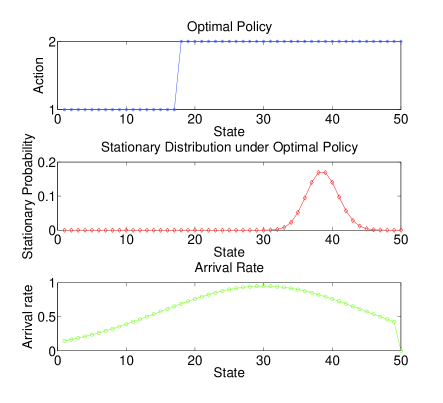
Figure 1: The true MDP for the queueing system simulation. (a) The optimal policy $c^{\star}$ selecting an action ($1,2$) for each state in $0,1,2,\ldots,50$. The optimal average reward is $96.4088$ units. (b) Stationary probability distribution for the optimal policy. (c) Parameterized (by a Gaussian curve), state-dependent, average arrival rate profile.

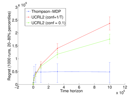
Figure 2: Regret for TSMDP and UCRL2 (Jaksch et al., 2010), across 1000 runs, for the single-queue parameterized MDP. Both mean regret and $[20,80]\%$-percentiles are shown.

7 Related Work

A line of recent work (Agrawal and Goyal, 2012; Kaufmann et al., 2012; Korda et al., 2013; Agrawal and Goyal, 2013; Gopalan et al., 2014) has demonstrated that the Thompson sampling enjoys near-optimal regret guarantees for multi-armed bandits – a widely studied subclass of reinforcement learning problems.

The work of Osband et al (Osband et al., 2013), perhaps the most relevant to us, studies the Bayesian regret of Thompson sampling for MDPs. In this setting, the true MDP is assumed to have been drawn from the same prior used by the algorithm; consequently, the Bayesian regret becomes the standard frequentist regret averaged across the entire parameter space w.r.t. the prior. While this is useful, it is arguably weaker than the standard frequentist notion of regret in that it is an averaged notion of standard regret (w.r.t. the specific prior), and moreover is not indicative of how the structure of the MDP exactly influences regret performance. Moreover, the learning model considered in their work is episodic with fixed-length episodes and resets, as opposed to the non-episodic learning setting treated in this work, where we are able to show the first known structural (“gap-dependent”) regret bounds for Thompson sampling in fixed but unknown parameterized MDPs.

Prior to this, Ortega and Braun (2010) investigate the consistency performance of posterior-sampling based control rules, again in the fully Bayesian setting where nature’s prior is known.

Several deterministic algorithms relying on the “optimism under uncertainty” philosophy have been proposed for RL in the frequentist setup considered here (Brafman and Tennenholtz, 2003; Jaksch et al., 2010; Bartlett and Tewari, 2009). These algorithms work by maintaining confidence intervals for each transition probability and reward, computing the most optimistic MDP satisfying all confidence intervals and adaptively shrinking the confidence intervals each time the relevant state transition occurs. This strategy is potentially inefficient in parameterized MDPs where, potentially, observing a particular state transition can give information about other parts of the MDP as well.

The parameterized MDP setting we consider in this work has been previously studied by other authors. Dyagilev et al (Dyagilev et al., 2008) investigate learning parameterized MDPs for finite parameter spaces in the discounted setting (we consider the average-reward setting), and demonstrate sample-complexity results under the Probably-Approximately-Correct (PAC) learning model, which is different from the notion of regret.

The certainty equivalence approach to learning MDPs (Kumar and Varaiya, 1986) – building the most plausible model given available data and using the optimal policy for it – is perhaps natural, but it suffers from a serious lack of adequate exploration necessary to achieve low regret (Kaelbling et al., 1996).

A noteworthy related work is the seminal paper of Agrawal et al (Agrawal et al., 1989) that gives fundamental lower bounds on the asymptotic regret scaling for general, parameterized reinforcement learning problems. The bound is also tight, in the sense that for finite parameter spaces, the authors show a learning algorithm that achieves the bound. Even though our analytical results also hold for the setting of a finite parameter space, the strategy in (Agrawal et al., 1989) relies crucially on the finiteness assumption. This is in sharp contrast to Thompson sampling which can be defined for any kind of parameter space. In fact, Thompson sampling has previously been shown to enjoy favorable regret guarantees with continuous priors in linear bandit problems (Agrawal and Goyal, 2013).

8 Conclusion and Future Work

We have proposed the TSMDP algorithm in this paper for solving parameterized RL problems, and have derived regret-style bounds for the algorithm under significantly general initial priors. This supports the increasing evidence for the success of Thompson sampling and pseudo-Bayesian methods for reinforcement learning/bandit problems.

Moving forward, it would be useful to extend the performance results for Thompson sampling to continuous parameter spaces, as well as understand what happens when feedback can be delayed. Specific applications to reinforcement learning problems with additional structure would also prove insightful. In particular, studying the regret of Thompson Sampling for MDPs with linear function approximation (Melo et al., 2008) would be of interest – in this setting, the parameterization of the MDP is in terms of linear weights corresponding to a known basis of state-action value functions, and one could develop a variant of Thompson sampling which uses information from sample paths to update its posterior over the space of weights.

Supplementary Material (Appendices and References)

Thompson Sampling for Learning Parameterized Markov Decision Processes

Appendix A Proof of Theorem 1

A.1 Expressing the “posterior” distribution

At time $t$, the “posterior distribution” $\pi_{t}$ that TSMDP uses can be expressed by iterating Bayes’ rule (1):

$$\forall\mathcal{M}\subseteq\Theta\quad\pi_{t}(\mathcal{M}) =\frac{W_{t}(\mathcal{M})}{W_{t}(\Theta)}=\frac{\int_{\mathcal{M}}W_{t}(\theta)\pi(d\theta)}{\int_{\Theta}W_{t}(\theta)\pi(d\theta)},$$

with the posterior density or weight $W_{t}(\theta)$ simply being the likelihood ratio of the entire observed history up to $t$ under the MDPs $m_{\theta}$ and $m_{\theta^{\star}}$, i.e.,

$$W_{t}(\theta):=\prod_{i=0}^{t-1}\frac{p_{\theta}(S_{i},A_{i+1},S_{i+1})}{p_{\theta^{\star}}(S_{i},A_{i+1},S_{i+1})}$$

$$=\exp\left(\sum_{c\in\mathcal{C}}\sum_{i=0}^{t-1}\mathbbm{1}\{C_{e(i)}=c\}\log\frac{p_{\theta}(S_{i},A_{i+1},S_{i+1})}{p_{\theta^{\star}}(S_{i},A_{i+1},S_{i+1})}\right)$$

$$=\exp\left(\sum_{c\in\mathcal{C}}\sum_{(s_{1},s_{2})\in\mathcal{S}^{2}}\sum_{i=0}^{t-1}\mathbbm{1}\left\{C_{e(i)}=c,(S_{i},S_{i+1})=(s_{1},s_{2})\right\}\log\frac{p_{\theta}(s_{1},c(s_{1}),s_{2})}{p_{\theta^{\star}}(s_{1},c(s_{1}),s_{2})}\right)$$

$$=\exp\left(-\sum_{c\in\mathcal{C}}V_{c}(t)\sum_{(s_{1},s_{2})\in\mathcal{S}^{2}}\sum_{i=0}^{t-1}\frac{\mathbbm{1}\left\{C_{e(i)}=c,(S_{i},S_{i+1})=(s_{1},s_{2})\right\}}{V_{c}(t)}\log\frac{p_{\theta^{\star}}(s_{1},c(s_{1}),s_{2})}{p_{\theta}(s_{1},c(s_{1}),s_{2})}\right),$$ (5)

where $V_{c}(t):=\sum_{i=0}^{t-1}\mathbbm{1}\left\{C_{e(i)}=c\right\}$ is the total number of time instants up to $t$ for which the epoch policy $c$ was used.

We will find it convenient in the sequel to introduce the following decomposition of the number of epochs up to epoch $k$ for which $c$ was chosen to be the epoch policy:

$$N_{c}(k):=\sum_{l=1}^{k}\mathbbm{1}\{\theta_{l}\in S_{c}\}=N_{c}^{\prime}(k)+N_{c}^{\prime\prime}(k),$$ (6)

$$N_{c}^{\prime}(k):=\sum_{l=1}^{k}\mathbbm{1}\{\theta_{l}\in S_{c}^{\prime}\},N_{c}^{\prime\prime}(k):=\sum_{l=1}^{k}\mathbbm{1}\{\theta_{l}\in S_{c}^{\prime\prime}\}.$$

A.2 An alternative probability space

In order to analyze the dynamics of the TSMDP algorithm, it is useful to work in an equivalent probability space defined as follows. Define a $\infty\times|\mathcal{C}|$ random matrix $Q$ with elements in $\mathcal{S}\times\mathcal{A}\times\mathbb{R}$. The rows of $Q$ are indexed by sampling indices $l=1,2,\ldots$, and the columns by policies in $\mathcal{C}$. For each $c\in\mathcal{C}$, independently generate the $c$-th column of $Q$ by applying the stationary policy $c$ to the MDP $m_{\theta^{\star}}$, starting from initial state $s_{0}$, and noting down the resulting $(state,action,reward)$ sequence, i.e., $Q(l,c)\equiv(Q_{1}(l,c),Q_{2}(l,c),Q_{3}(l,c)):=({S}^{\theta^{\star},c}_{l},{A}^{\theta^{\star},c}_{l},{R}^{\theta^{\star},c}_{l})$. For the $c$-th column of $Q$, we let $\tilde{\tau}_{0,c}:=0$, and $\tilde{\tau}_{k,c}:=\min\{l\geq\tilde{\tau}_{k-1,c}:Q_{1}(l,c)=s_{0}\}$ $\forall k\geq 1$. In words, $\tilde{\tau}_{k,c}$ is the $k$-th successive “virtual time” at which the MDP $m_{\theta^{\star}}$ under policy $c$ returns to the start state $s_{0}$. We thus have that the expected first return time to $s_{0}$, defined earlier in Section 3, satisfies $\bar{\tau}_{c}=\tilde{\mathbb{E}}[\tilde{\tau}_{1,c}]$.

Given the matrix $Q$, we can alternatively simulate the TSMDP algorithm operating in the MDP $m_{\theta^{\star}}$ as follows. At each round $t\geq 1$ with the epoch index $e(t)=k$, if the epoch policy in effect is $C_{k}=c$, then the action $A_{t}=Q_{2}(\tilde{\tau}_{N_{c}(k),c}+t-t_{k},c)$ is played, with the next state (resp. reward) being $S_{t}=Q_{1}(\tilde{\tau}_{N_{c}(k),c}+t-t_{k},c)$ (resp. $R_{t}=Q_{3}(\tilde{\tau}_{N_{c}(k),c}+t-t_{k},c)$).

Let $\tilde{\mathbb{P}}$ denote the probability measure for the alternative probability space described above. The following equivalence lemma records the fact that the distributions of the $(state,action,reward)$ sample path seen by the TSMDP algorithm under the original probability measure $\mathbb{P}$ and under in the alternative measure $\tilde{\mathbb{P}}$ are both identical.

Lemma 1 (Equivalence of probability spaces).

For each $(state,action,reward)$ sequence
$\{(s_{t},a_{t},r_{t})\}_{t=1}^{T}$, we have, under the TSMDP algorithm,

$$\tilde{\mathbb{P}}\left[\forall 1\leq t\leq T\;(S_{t},A_{t},R_{t})=(s_{t},a_{t},r_{t})\right]=\mathbb{P}\left[{\forall 1\leq t\leq T\;(S_{t},A_{t},R_{t})=(s_{t},a_{t},r_{t})}\right].$$

Henceforth, we will work in the alternative space with measure $\tilde{\mathbb{P}}$ but will dispense with the tilde for ease of notation.

We now develop some useful concentration estimates for the random sample path matrix $Q$. Define the following empirical estimates:

• $U_{(s_{1},s_{2})}(j,c):=\frac{1}{j}\sum_{l=1}^{j}\mathbbm{1}\left\{Q_{1}(l-1,c)=s_{1},Q_{1}(l,c)=s_{2}\right\}$, $s_{1},s_{2}\in\mathcal{S}$, $j\geq 1$, denote the empirical mean number of state transitions $s_{1}\rightarrow s_{2}$ down column $c$ of $Q$ (or the pairwise empirical frequency),

• $U(j,c):=\left(U_{(s_{1},s_{2})}(j,c)\right)_{s_{1},s_{2}\in\mathcal{S}}$ denote the empirical state transition vector for policy $c$,

• $U_{s_{1}}(j,c):=\sum_{s_{2}\in\mathcal{S}}U_{(s_{1},s_{2})}(j,c)$, $s_{1}\in\mathcal{S}$, $j\geq 1$, be the marginal empirical frequency, and

• $U_{s_{2}|s_{1}}(j,c):=\frac{U_{(s_{1},s_{2})}(j,c)}{U_{s_{1}}(j,c)}$, $s_{1}\in\mathcal{S}$, $s_{2}\in\mathcal{S}$, $j\geq 1$, be the conditional empirical frequency (whenever $U_{s_{1}}(j,c)>0$; defined to be $0$ otherwise)

in $j$ virtual time steps. With this alternative view of the TSMDP execution, equation (5) for the posterior probability density $W_{t}$ at time $t$ becomes

$$-\log W_{t}(\theta)=\sum_{c\in\mathcal{C}}V_{c}(t)\sum_{(s_{1},s_{2})\in\mathcal{S}^{2}}U_{(s_{1},s_{2})}\left(V_{c}(t),c\right)\log\frac{p_{\theta^{\star}}(s_{1},c(s_{1}),s_{2})}{p_{\theta}(s_{1},c(s_{1}),s_{2})}.$$ (7)

The following key self-normalized uniform bound controls the large deviation behavior of the empirical means $U_{(s_{1},s_{2})}(j,c)$ and the return times $\tilde{\tau}_{k,c}$. It may be interpreted as a finite-sample version of the Law of the Iterated Logarithm (LIL).

Proposition 1 (Uniform concentration for empirical means).

Fix $\delta\in[0,1]$. Then, there exist constants $d_{1}\geq 0$, $d_{2}\geq 0$ such that the following estimates hold with probability at least $1-\delta$ for all $k\geq 1$, $c\in\mathcal{C}$, $s_{1},s_{2}\in\mathcal{S}$:

$$\left|\tilde{\tau}_{k,c}-k\bar{\tau}_{c}\right|\leq\sqrt{kd_{1}\log\left(\frac{|\mathcal{C}||\mathcal{S}|^{2}d_{2}\log k}{\delta}\right)},$$ (8)

$$\left|\tilde{\tau}_{k,c}\cdot U_{(s_{1},s_{2})}(\tilde{\tau}_{k,c},c)-k\bar{\tau}_{c}\cdot{\pi^{(c)}_{(s_{1},s_{2})}}\right|\leq\sqrt{kd_{1}\log\left(\frac{|\mathcal{C}||\mathcal{S}|^{2}d_{2}\log k}{\delta}\right)},$$ (9)

$$\left|\tilde{\tau}_{k,c}\cdot U_{s_{1}}(\tilde{\tau}_{k,c},c)-k\bar{\tau}_{c}\cdot{\pi^{(c)}_{s_{1}}}\right|\leq\sqrt{kd_{1}\log\left(\frac{|\mathcal{C}||\mathcal{S}|^{2}d_{2}\log k}{\delta}\right)}.$$ (10)

Proof.

By the Markov property, it follows that the (non-negative) random variables $\tilde{\tau}_{1,c}$, $(\tilde{\tau}_{2,c}-\tilde{\tau}_{1,c})$, $(\tilde{\tau}_{3,c}-\tilde{\tau}_{2,c})$, $\ldots$, $(\tilde{\tau}_{k,c}-\tilde{\tau}_{k-1,c})$ are IID. From standard arguments for finite-state, irreducible Markov chains Lee et al. (2013, Lemma 7), we have that the recurrence times to $s_{0}$ have exponential tails:

$$\forall v\geq 0\quad\mathbb{P}\left[{\tilde{\tau}_{1,c}>v}\right]\leq 2\cdot 2^{-\left(\frac{v}{2\bar{\tau}_{\max}}\right)},$$ (11)

where $\bar{\tau}_{\max}$ is the maximum expected hitting time, over states in the same communicating class as $s_{0}$, to $s_{0}$. We also have $\mathbb{E}\left[{\tilde{\tau}_{1,c}}\right]=\bar{\tau}_{c}$.

On the other hand, using the definition of $U_{(s_{1},s_{2})}(\tilde{\tau}_{k,c},c)$, we can write

$$\tilde{\tau}_{k,c}\cdot U_{(s_{1},s_{2})}(\tilde{\tau}_{k,c},c)=\sum_{j=1}^{k}B_{c,s_{1},s_{2}}(\tilde{\tau}_{j-1,c}+1,\tilde{\tau}_{j,c}),$$

where the partial sums

$$B_{c,s_{1},s_{2}}(\tilde{\tau}_{j-1,c}+1,\tilde{\tau}_{j,c}):=\sum_{l=\tilde{\tau}_{j-1,c}+1}^{\tilde{\tau}_{j,c}}\mathbbm{1}\left\{Q_{1}(l-1)=s_{1},Q_{1}(l)=s_{2}\right\},\quad j=1,2,\ldots,k$$

are again non-negative IID random variables due to the Markov property, and are bounded by the corresponding cycle lengths $(\tilde{\tau}_{j,c}-\tilde{\tau}_{j-1,c})$. Thus, $B_{c,s_{1},s_{2}}(1,\tilde{\tau}_{1,c})$ also satisfies the exponential tail inequality (11) satisfied by $\tilde{\tau}_{1,c}$, with mean $\mathbb{E}\left[{B_{c,s_{1},s_{2}}(1,\tilde{\tau}_{1,c})}\right]=\frac{\pi^{(c)}_{(s_{1},s_{2})}}{\pi_{s_{0}}(\theta^{\star},c)}=\bar{\tau}_{c}\cdot{\pi^{(c)}_{(s_{1},s_{2})}}$.

The conclusions of the proposition now follow by (a) appealing to the maximal concentration inequality of Lemma 2, and (b) taking a union bound over all $c\in\mathcal{C}$, $s_{1},s_{2}\in\mathcal{S}$ with the least possible uniform upper bounds on the constants $\eta_{1}$ and $\eta_{2}$ guaranteed by Lemma 2. ∎

Lemma 2 below gives a concentration bound for the entire sample path of the empirical mean of an IID process, and may be viewed as a finite-sample analog of the asymptotic Law of the Iterated Logarithm (LIL).

Lemma 2 (A maximal concentration inequality for random walks with sub-exponential increments).

Let $X_{1},X_{2},\ldots$ be a sequence of IID random variables such that $\mathbb{P}\left[{|X_{1}|>v}\right]\leq\alpha_{1}e^{-\alpha_{2}v}$ for some $\alpha_{1},\alpha_{2}>0$, and fix $\delta\in[0,1]$. Then, there exist constants $\eta_{1}\geq 0$, $\eta_{2}\geq 0$ such that the following event occurs with probability at least $1-\delta$:

$$\forall{k\geq 1}\;\left|\sum_{i=1}^{k}X_{i}-k\mathbb{E}\left[{X_{1}}\right]\right|\leq\sqrt{\eta_{1}k\log\left(\frac{\eta_{2}\log k}{\delta}\right)}.$$

Proof.

We begin by noticing that the exponential tail property implies finiteness of the moment generating function in a neighborhood of zero: for any $\lambda\in(0,\alpha_{2})$,

$$e^{\Lambda_{X_{1}}(\lambda)}:=\mathbb{E}\left[{e^{\lambda X_{1}}}\right] =\int_{0}^{\infty}\mathbb{P}\left[{e^{\lambda X_{1}}>y}\right]dy$$

$$\leq 1+\int_{1}^{\infty}\mathbb{P}\left[{e^{\lambda X_{1}}>y}\right]dy$$

$$\leq 1+\int_{1}^{\infty}\alpha_{1}y^{-\alpha_{2}/\lambda}dy<\infty.$$

This allows us to take a second-order Taylor series expansion of $\Lambda_{X_{1}}(\lambda)$ around $\lambda=0$, to get that $\exists\beta\in\mathbb{R}$ such that $\Lambda_{X_{1}}(\lambda)\leq\lambda\mathbb{E}\left[{X_{1}}\right]+\frac{\beta^{2}\lambda^{2}}{2}$ $\forall\lambda\in\left[-\frac{\alpha_{2}}{2},\frac{\alpha_{2}}{2}\right]$. As a consequence,

$$M_{t}:=\exp\left(\lambda\sum_{i=1}^{t}X_{i}-\lambda t\mathbb{E}\left[{X_{1}}\right]-\frac{t\beta^{2}\lambda^{2}}{2}\right),\quad t=0,1,2,\ldots$$

is a non-negative supermartingale for each $\lambda\in\left[-\frac{\alpha_{2}}{2},\frac{\alpha_{2}}{2}\right]$. Applying the method of mixtures technique for martingale suprema (de la Peña et al., 2007, Example 2.5) (due, in turn, to the pioneering work of Robbins and Siegmund (1970, Example 4)), we obtain the bound

$$\mathbb{P}\left[{\sum_{i=1}^{k}X_{i}-k\mathbb{E}\left[{X_{1}}\right]\geq g_{k}\quad\mbox{for some }k\geq 1}\right]\leq\delta,$$

with $g_{k}:=\sqrt{\gamma_{2}\beta^{2}k\log\left(\frac{\gamma_{1}\log(\beta^{2}k)}{\delta}\right)}$ for some constants $\gamma_{1}\geq 0$, $\gamma_{2}\geq 0$. This finishes one half of the proof for the “positive tail” $\sum_{i=1}^{k}X_{i}$ . The other half follows in an analogous fashion by considering the negated random variables $\{-X_{i}\}_{i}$. ∎

We henceforth consider as fixed the confidence parameter $\delta\in[0,1]$, and denote $\rho(x)\equiv\rho_{\delta}(x):=\sqrt{d_{1}\log\left(\frac{|\mathcal{C}||\mathcal{S}|^{2}d_{2}\log x}{\delta}\right)}$, $x\geq 1$. Note that $\rho(x)=O\left(\sqrt{\log\log(x)}\right)$ as a function of $x$.

Definition 1 (“Typical” trajectories).

Let

$$G:=\left\{\begin{array}[]{ll}&\left|\tilde{\tau}_{k,c}-k\bar{\tau}_{c}\right|\leq\rho(k)\sqrt{k},\\ \forall c\in\mathcal{C}\;\forall s_{1},s_{2}\in\mathcal{S}\;\forall k\geq 1:&\left|\tilde{\tau}_{k,c}U_{(s_{1},s_{2})}(\tilde{\tau}_{k,c},c)-k\bar{\tau}_{c}{\pi^{(c)}_{(s_{1},s_{2})}}\right|\leq\rho(k)\sqrt{k},\\ &\left|\tilde{\tau}_{k,c}U_{s_{1}}(\tilde{\tau}_{k,c},c)-k\bar{\tau}_{c}{\pi^{(c)}_{s_{1}}}\right|\leq\rho(k)\sqrt{k}\end{array}\right\}$$

be the event that the random matrix $Q$ from Section A.2 satisfies (8) and (9) (“near-ideal” sample paths).

We thus have, by our previous estimates, that

$$\mathbb{P}\left[{G}\right]\geq 1-\delta.$$ (12)

The crux of the proof of Theorem 1 is in controlling regret of two kinds.

1. Regret due to sampling parameters from $S_{c}^{\prime\prime}$, $c\neq c^{\star}$: We will show that the true parameter $\theta^{\star}$ is sampled at least a constant fraction (bounded away from $0$) of times in $0,1,\ldots,T$. This implies that parameters in $S_{c}^{\prime\prime}$ are sampled at most a constant number of times.

2. Regret due to sampling parameters from $S_{c}^{\prime},c\neq c^{\star}$: We will establish that the number of times that parameters from $S_{c}^{\prime}$ are sampled is the claimed logarithmic bound in Theorem 1.

A.3 Regret due to sampling from $S_{c}^{\prime\prime}$

In this section, our goal is to show

Proposition 2 ($O(1)$ samples from $S_{c}^{\prime\prime}$ whp.).

There exists $\alpha<\infty$ such that

$$\mathbb{P}\left[{\exists c\neq c^{\star}\;\sum_{k=1}^{\infty}\mathbbm{1}\{\theta_{k}\in S_{c}^{\prime\prime}\}>\frac{\alpha|\mathcal{C}|}{\delta}\;\big{|}\;G}\right]\leq\delta.$$

Let $J_{(s_{1},s_{2})}(k_{c},c)$ denote the number of instants that the state transition $s_{1}\to s_{2}$ occurs in $k_{c}$ successive epoch uses of policy $c$.

Lemma 3.

Under the event $G$, for each $\theta\in\Theta$ satisfying $\pi(\theta)>0$, each $c\in\mathcal{C}$ and $k\geq 1$,

1. The following lower bound holds on the negative log-density.

   $$-\log W_{t_{k}}(\theta)\geq N_{c}(k)\bar{\tau}_{c}\cdot D_{c}(\theta^{\star}||\theta)-\Gamma|\mathcal{S}|^{2}\rho(N_{c}(k))\sqrt{N_{c}(k)}.$$

2. The following upper bound holds on the negative log-density.

   $$-\log W_{t_{k}}(\theta)\leq N_{c}(k)\bar{\tau}_{c}\cdot D_{c}(\theta^{\star}||\theta)+\Gamma|\mathcal{S}|^{2}\rho(N_{c}(k))\sqrt{N_{c}(k)}.$$

Proof.

Since $t_{k}$ is an epoch boundary, $V_{c}(t_{k})=\tilde{\tau}_{k^{\prime}_{c},c}$ for $k^{\prime}_{c}:=N_{c}(k)$. Using (7), we can write

$$-\log W_{t_{k}}(\theta) =V_{c}(t_{k})\sum_{(s_{1},s_{2})\in\mathcal{S}^{2}}U_{(s_{1},s_{2})}\left(V_{c}(t_{k}),c\right)\log\frac{p_{\theta^{\star}}(s_{1},c(s_{1}),s_{2})}{p_{\theta}(s_{1},c(s_{1}),s_{2})}$$

$$=\sum_{(s_{1},s_{2})\in\mathcal{S}^{2}}\tilde{\tau}_{k^{\prime}_{c},c}\cdot U_{(s_{1},s_{2})}\left(\tilde{\tau}_{k^{\prime}_{c},c},c\right)\log\frac{p_{\theta^{\star}}(s_{1},c(s_{1}),s_{2})}{p_{\theta}(s_{1},c(s_{1}),s_{2})}$$

$$=\sum_{(s_{1},s_{2})\in\mathcal{S}^{2}}\left[\tilde{\tau}_{k^{\prime}_{c},c}\cdot U_{(s_{1},s_{2})}\left(\tilde{\tau}_{k^{\prime}_{c},c},c\right)-k^{\prime}_{c}\bar{\tau}_{c}\cdot{\pi^{(c)}_{(s_{1},s_{2})}}\right]\log\frac{p_{\theta^{\star}}(s_{1},c(s_{1}),s_{2})}{p_{\theta}(s_{1},c(s_{1}),s_{2})}$$

$$\quad\quad\quad\quad+\sum_{(s_{1},s_{2})\in\mathcal{S}^{2}}k^{\prime}_{c}\bar{\tau}_{c}\cdot{\pi^{(c)}_{(s_{1},s_{2})}}\log\frac{p_{\theta^{\star}}(s_{1},c(s_{1}),s_{2})}{p_{\theta}(s_{1},c(s_{1}),s_{2})}$$

$$\geq-\sum_{(s_{1},s_{2})\in\mathcal{S}^{2}}\rho(k^{\prime}_{c})\sqrt{k^{\prime}_{c}}\cdot\left|\log\frac{p_{\theta^{\star}}(s_{1},c(s_{1}),s_{2})}{p_{\theta}(s_{1},c(s_{1}),s_{2})}\right|$$

$$\quad\quad\quad\quad+k^{\prime}_{c}\bar{\tau}_{c}\sum_{s_{1}\in\mathcal{S}}\pi^{(c)}_{s_{1}}\sum_{s_{2}\in\mathcal{S}}\frac{\pi^{(c)}_{(s_{1},s_{2})}}{\pi^{(c)}_{s_{1}}}\log\frac{p_{\theta^{\star}}(s_{1},c(s_{1}),s_{2})}{p_{\theta}(s_{1},c(s_{1}),s_{2})}$$

$$\geq k^{\prime}_{c}\bar{\tau}_{c}\cdot D_{c}(\theta^{\star}||\theta)-\Gamma|\mathcal{S}|^{2}\rho(k^{\prime}_{c})\sqrt{k^{\prime}_{c}},$$ (13)

where the final line is by the definition of event $G$ and by using Assumption 2. This proves the first assertion of the lemma. The second assertion follows in a similar fashion. ∎

Lemma 4 (Bounded ratio of Log-likelihood and KL-divergence).

Denote, for policy $c\in\mathcal{C}$ and parameter $\theta\in\Theta$,

$$L_{c}(\theta):=\sum_{(s_{1},s_{2})\in\mathcal{S}^{2}}\left|\log\frac{p_{\theta^{\star}}(s_{1},c(s_{1}),s_{2})}{p_{\theta}(s_{1},c(s_{1}),s_{2})}\right|.$$

There exists a universal constant $g$ such that

$$\sup_{\begin{subarray}{c}\theta\in\Theta,c\in\mathcal{C}\\ D_{c}(\theta^{\star}||\theta)>0\end{subarray}}\frac{L_{c}(\theta)}{\sqrt{D_{c}(\theta^{\star}||\theta)}}\leq g<\infty.$$

Proof.

By Assumption 2, $L_{c}(\theta)\leq\Gamma|\mathcal{S}|^{2}$, so it only suffices to bound from above the ratio $L_{c}(\theta)/D_{c}(\theta^{\star}||\theta)$ for $\theta\to\theta^{\star}$. In this case, it is not hard to see that for $\theta=\theta^{\star}+\delta^{\prime}$ for $|\delta^{\prime}|$ small enough, $L_{c}(\theta)=O(\delta^{\prime})$ while $D_{c}(\theta^{\star}||\theta)=O({\delta^{\prime}}^{2})$. Hence, the ratio $L_{c}(\theta)/D_{c}(\theta^{\star}||\theta)$ is bounded above by a universal constant, which completes the proof of the lemma. ∎

Let $\Theta_{1}:=\{\theta\in\Theta:\sum_{c\in\mathcal{C}}N_{c}(k)\bar{\tau}_{c}D_{c}(\theta^{\star}||\theta)\leq 1\}$. By Assumption 5A, $\pi(\Theta_{1})\geq a_{1}k^{-a_{2}}$.

By the penultimate inequality in the derivation of Lemma 3, we have that under the event $G$, for any $\theta\in\Theta_{1}$,

$$-\log W_{t_{k}}(\theta) \leq\sum_{c\in\mathcal{C}}N_{c}(k)\bar{\tau}_{c}D_{c}(\theta^{\star}||\theta)+\sum_{c\in\mathcal{C}}\rho(N_{c}(k))\sqrt{N_{c}(k)}L_{c}(\theta)$$

$$\leq 1+\sum_{c\in\mathcal{C}}\rho(N_{c}(k))\sqrt{N_{c}(k)}L_{c}(\theta)\quad\mbox{(since $\theta\in\Theta_{1}$)}$$

$$\leq 1+\sqrt{\sum_{c\in\mathcal{C}}N_{c}(k)\bar{\tau}_{c}D_{c}(\theta^{\star}||\theta)}\sqrt{\sum_{c\in\mathcal{C}}\frac{\rho^{2}(N_{c}(k))}{\bar{\tau}_{c}}\cdot\frac{L_{c}^{2}(\theta)}{D_{c}(\theta^{\star}||\theta)}}\quad\mbox{(Cauchy-Schwarz inequality)}$$

$$\leq 1+\rho(k)\sqrt{\sum_{c\in\mathcal{C}}\frac{L_{c}^{2}(\theta)}{D_{c}(\theta^{\star}||\theta)}}\quad\mbox{(since $\bar{\tau}_{c}\geq 1$ $\forall c\in\mathcal{C}$)}$$

$$\leq 1+\rho(k)g\sqrt{|\mathcal{C}|},$$

where $g$ is the constant guaranteed by Lemma 4. Thus, under $G$,

$$\int_{\Theta}W_{t_{k}}(\theta^{\prime})\pi(d\theta^{\prime}) \geq\int_{\Theta_{1}}W_{t_{k}}(\theta^{\prime})\pi(d\theta^{\prime})$$

$$\geq\int_{\Theta_{1}}e^{-1-\rho(k)g\sqrt{|\mathcal{C}|}}\;\pi(d\theta^{\prime})$$

$$=e^{-1-\rho(k)g\sqrt{|\mathcal{C}|}}\;\pi(\Theta_{1})$$

$$\geq e^{-1-\rho(k)g\sqrt{|\mathcal{C}|}}a_{1}k^{-a_{2}}\geq a_{1}^{\prime}k^{-a_{2}^{\prime}}$$ (14)

for some suitable constants $a_{1}^{\prime},a_{2}^{\prime}$.

We proceed to bound from above the posterior probability of $S_{c}^{\prime\prime}$, $c\neq c^{\star}$ under the event $G$. To this end, write

$$\frac{W_{t_{k}}(\theta)}{\int_{\Theta}W_{t_{k}}(\theta^{\prime})\pi(d\theta^{\prime})}\leq\frac{W_{t_{k}}(\theta)}{a_{1}^{\prime}k^{-a_{2}^{\prime}}}$$

$$=\frac{1}{a_{1}^{\prime}k^{-a_{2}^{\prime}}}\exp\left[-\sum_{c\in\mathcal{C}}V_{c}(t_{k})\sum_{s_{1},s_{2}}U_{(s_{1},s_{2})}\left(V_{c}(t_{k}),c\right)\log\frac{p_{\theta^{\star}}(s_{1},c(s_{1}),s_{2})}{p_{\theta}(s_{1},c(s_{1}),s_{2})}\right]$$

$$\leq\frac{1}{a_{1}^{\prime}k^{-a_{2}^{\prime}}}\exp\left[-N_{c^{\star}}(k)\bar{\tau}_{{c^{\star}}}\cdot D_{c^{\star}}(\theta^{\star}||\theta)+\Gamma|\mathcal{S}|^{2}\rho(N_{c^{\star}}(k))\sqrt{N_{c^{\star}}(k)}\right],$$

where, from Section 3, $N_{c^{\star}}(k)$ is the number of epochs up until epoch $k$ (i.e., until time instant $t_{k}$) in which the optimal policy $c^{\star}$ is chosen. The first inequality is by (14). The second inequality results by applying the conclusion of Lemma 3 to all policies $c\neq c^{\star}$. Using the uniform lower bound $D_{c^{\star}}(\theta^{\star}||\theta)\geq\epsilon^{\prime}$ $\forall\theta\in S_{c}^{\prime\prime}$ and integrating the above inequality over $\theta\in S_{c}^{\prime\prime}$ gives the bound

$$\pi_{t_{k}}(S_{c}^{\prime\prime})\leq\nu_{k}\exp\left[-\epsilon^{\prime}N_{c^{\star}}(k)\bar{\tau}_{{c^{\star}}}+\Gamma|\mathcal{S}|^{2}\rho(N_{c^{\star}}(k))\sqrt{N_{c^{\star}}(k)}\right],$$

with $\nu_{k}:=\frac{1}{a_{1}^{\prime}k^{-a_{2}^{\prime}}}$. The key property of the above estimate is that it decays exponentially with $N_{c^{\star}}(k)$. (Intuitively, since $\theta^{\star}$ is sampled with frequency at least $p^{\star}$, we expect that $N_{c^{\star}}(k)\approx kp^{\star}$, and thus the estimate is also exponential in $k$.)

Proof of Proposition 2.

We begin by estimating the moment generating function of $N_{c^{\star}}(k)$. Let $\mathcal{F}_{t}$ denote the $\sigma$-algebra generated by the history of the algorithm up to time $t$ and state $S_{t}$, i.e., the $\sigma$-algebra generated by the random variables

$$\left\{(S_{0},A_{0},R_{0}),\ldots,(S_{t-1},A_{t-1},R_{t-1}),S_{t}\right\}.$$

We have

$$\mathbb{E}\left[{e^{-\epsilon^{\prime}N_{c^{\star}}(k)}\;\big{|}\;G}\right] =\mathbb{E}\left[{\mathbb{E}\left[{e^{-\epsilon^{\prime}N_{c^{\star}}(k)}\;\big{|}\;\mathcal{F}_{t_{k-1}},G}\right]\;\big{|}\;G}\right]$$

$$=\mathbb{E}\left[{e^{-\epsilon^{\prime}N_{c^{\star}}(k-1)}\mathbb{E}\left[{e^{-\epsilon^{\prime}\mathbbm{1}\{C_{k}=c^{\star}\}}\;\big{|}\;\mathcal{F}_{t_{k}},G}\right]\;\big{|}\;G}\right]$$

$$\leq\mathbb{E}\left[{e^{-\epsilon^{\prime}N_{c^{\star}}(k-1)}\mathbb{E}\left[{e^{-\epsilon^{\prime}\mathbbm{1}\{\theta_{t_{k}}\in S_{c^{\star}}\}}\;\big{|}\;\mathcal{F}_{t_{k}},G}\right]\;\big{|}\;G}\right]$$

$$\leq\mathbb{E}\left[{e^{-\epsilon^{\prime}N_{c^{\star}}(k-1)}\left(p^{\star}e^{-\epsilon^{\prime}}+1-p^{\star}\right)\;\big{|}\;G}\right]$$

$$=\left(p^{\star}e^{-\epsilon^{\prime}}+1-p^{\star}\right)\mathbb{E}\left[{e^{-\epsilon^{\prime}N_{c^{\star}}(k-1)}\;\big{|}\;G}\right],$$

where, in the penultimate step, we have used the fact that the probability of sampling $\theta^{\star}$ under $G$ is at least $p^{\star}$ at all epoch boundaries (Assumption 4). Iterating the estimate further gives

$$\mathbb{E}\left[{e^{-\epsilon^{\prime}N_{c^{\star}}(k)}\;\big{|}\;G}\right]\leq\left(p^{\star}e^{-\epsilon^{\prime}}+1-p^{\star}\right)^{k}.$$

Using this with the conditional version of Markov’s inequality, we have, for $c\neq c^{\star}$ and $\chi>0$,

$$\mathbb{P}\left[{\sum_{k=1}^{\infty}\mathbbm{1}\{\theta_{k}\in S_{c}^{\prime\prime}\}>\chi\;\big{|}\;G}\right]\leq\chi^{-1}\mathbb{E}\left[{\sum_{k=1}^{\infty}\mathbbm{1}\{\theta_{k}\in S_{c}^{\prime\prime}\}>\chi\;\big{|}\;G}\right]$$

$$=\chi^{-1}\sum_{k=1}^{\infty}\mathbb{E}\left[{\mathbbm{1}\{\theta_{k}\in S_{c}^{\prime\prime}\}>\chi\;\big{|}\;G}\right]$$

$$\leq\chi^{-1}\sum_{k=1}^{\infty}\left(1\wedge\mathbb{E}\left[{\nu_{k}e^{-\epsilon^{\prime}N_{c^{\star}}(k)\bar{\tau}_{{c^{\star}}}+\Gamma|\mathcal{S}|^{2}\rho(N_{c^{\star}}(k))\sqrt{N_{c^{\star}}(k)}}\;\big{|}\;G}\right]\right)$$

$$\leq\chi^{-1}\sum_{k=1}^{\infty}\left(1\wedge\mathbb{E}\left[{\nu_{k}e^{-\epsilon^{\prime}N_{c^{\star}}(k)\bar{\tau}_{{c^{\star}}}+\Gamma|\mathcal{S}|^{2}\rho(k)\sqrt{k}}\;\big{|}\;G}\right]\right)$$

$$\leq\chi^{-1}\sum_{k=1}^{\infty}\left(1\wedge\nu_{k}\left(p^{\star}e^{-\epsilon^{\prime}}+1-p^{\star}\right)^{k}e^{\Gamma|\mathcal{S}|^{2}\rho(k)\sqrt{k}}\right).$$

Note that since $p^{\star}$ and $\epsilon^{\prime}$ are positive, $p^{\star}e^{-\epsilon^{\prime}}+1-p^{\star}<1$. Moreover, since both $\rho(k)\sqrt{k}=o(k)$ and $\log\nu_{k}=o(k)$, the sum above is dominated by a convergent geometric series after finitely many $k$, and is thus a finite quantity $\alpha<\infty$. Taking a union bound over all $c\neq c^{\star}$ completes the proof of Proposition 2. ∎

A.4 Regret due to sampling from $S_{c}^{\prime}$

We now turn to bounding the number of times that parameters from $S_{c}^{\prime}$ with $c\neq c^{\star}$ are sampled by the TSMDP algorithm.

We begin with the following key lemma, which helps to give a more refined estimate of the posterior weight exponent compared to Lemma 3.

Lemma 5.

Fix $\epsilon\in(0,1)$. By Assumption 1 and Lemma 4, it holds under the event $G$ that for each $\theta\in\Theta$, $c\in\mathcal{C}$ and $T\geq n\geq 1$,

$$V_{c}(t_{k})\sum_{(s_{1},s_{2})\in\mathcal{S}^{2}} U_{(s_{1},s_{2})}\left(V_{c}(t_{k}),c\right)\log\frac{p_{\theta^{\star}}(s_{1},c(s_{1}),s_{2})}{p_{\theta}(s_{1},c(s_{1}),s_{2})}$$

$$\geq(1-\epsilon)N_{c}(k)\bar{\tau}_{c}D_{c}(\theta^{\star}||\theta)-\frac{g^{2}d_{1}}{4\epsilon}\log\left(\frac{|\mathcal{C}||\mathcal{S}|^{2}d_{2}\log T}{\delta}\right).$$

The usefulness of the result stems from the fact that the left-hand term (which in fact helps to form the posterior log-density of $\theta$) can be approximated by a constant fraction of the marginal KL divergence $D_{c}(\theta^{\star}||\theta)$, with the approximation error being only $O\left(\frac{\log\log T}{\epsilon}\right)$.

Proof.

Denote $L_{c}(\theta):=\sum_{(s_{1},s_{2})\in\mathcal{S}^{2}}\left|\log\frac{p_{\theta^{\star}}(s_{1},c(s_{1}),s_{2})}{p_{\theta}(s_{1},c(s_{1}),s_{2})}\right|$. By the penultimate inequality in the derivation of Lemma 3, we have that under the event $G$,

$$V_{c}(t_{k})\sum_{(s_{1},s_{2})\in\mathcal{S}^{2}}U_{(s_{1},s_{2})}\left(V_{c}(t_{k}),c\right)\log\frac{p_{\theta^{\star}}(s_{1},c(s_{1}),s_{2})}{p_{\theta}(s_{1},c(s_{1}),s_{2})}$$

$$\geq k^{\prime}_{c}\bar{\tau}_{c}\cdot D_{c}(\theta^{\star}||\theta)-\rho(k^{\prime}_{c})\sqrt{k^{\prime}_{c}}\sum_{(s_{1},s_{2})\in\mathcal{S}^{2}}\left|\log\frac{p_{\theta^{\star}}(s_{1},c(s_{1}),s_{2})}{p_{\theta}(s_{1},c(s_{1}),s_{2})}\right|,$$

where $k^{\prime}_{c}:=N_{c}(k)$. The right hand side of the inequality above is of the form $ax-b\rho(x)\sqrt{x}$ if we identify $x\equiv k^{\prime}_{c}\in[0,T]$, $a\equiv\bar{\tau}_{c}\cdot D_{c}(\theta^{\star}||\theta)$ and $b\equiv L_{c}(\theta)$. To prove the lemma, it is enough to find $\gamma$ such that $ax-b\rho(x)\sqrt{x}\geq(1-\epsilon)ax-\gamma$ for every choice of $\theta\in\Theta$ and $c\in\mathcal{C}$. This is equivalent to requiring that $\gamma\geq-\epsilon ax+b\rho(x)\sqrt{x}$. Consider now

$$\sup_{T\geq x\geq 0}\left[-\epsilon ax+b\rho(x)\sqrt{x}\right]\leq\sup_{T\geq x\geq 0}\left[-\epsilon ax+b\sqrt{d_{1}x\log\left(\frac{|\mathcal{C}||\mathcal{S}|^{2}d_{2}\log x}{\delta}\right)}\right]$$

$$\leq\sup_{T\geq x\geq 0}\left[-\epsilon ax+b\sqrt{d_{1}x\log\left(\frac{|\mathcal{C}||\mathcal{S}|^{2}d_{2}\log T}{\delta}\right)}\right]$$

$$\leq\sup_{x\in\mathbb{R}}\left[-\epsilon ax+b\sqrt{d_{1}x\log\left(\frac{|\mathcal{C}||\mathcal{S}|^{2}d_{2}\log T}{\delta}\right)}\right]$$

$$=\frac{b^{2}{d_{1}\log\left(\frac{|\mathcal{C}||\mathcal{S}|^{2}d_{2}\log T}{\delta}\right)}}{4\epsilon a},$$

where the final step simply finds the maximum of the quadratic function over $x$. The only quantities depending on $\theta$ in the right hand side above are $a$ and $b$, so maximizing over $\theta\in\Theta$ for which $a\equiv\bar{\tau}_{c}\cdot D_{c}(\theta^{\star}||\theta)>0$, we further obtain

$$\sup_{\begin{subarray}{c}\theta\in\Theta,c\in\mathcal{C}\\ D_{c}(\theta^{\star}||\theta)>0\end{subarray}}\sup_{T\geq x\geq 0}\left[-\epsilon ax+b\rho(x)\sqrt{x}\right]\leq\frac{d_{1}}{4\epsilon}\log\left(\frac{|\mathcal{C}||\mathcal{S}|^{2}d_{2}\log T}{\delta}\right)\sup_{\begin{subarray}{c}\theta\in\Theta,c\in\mathcal{C}\\ D_{c}(\theta^{\star}||\theta)>0\end{subarray}}\left(\frac{L_{c}^{2}(\theta)}{\bar{\tau}_{c}D_{c}(\theta^{\star}||\theta)}\right)$$

$$\leq\frac{g^{2}d_{1}}{4\epsilon}\log\left(\frac{|\mathcal{C}||\mathcal{S}|^{2}d_{2}\log T}{\delta}\right),$$

where we have used Assumption 1 and Lemma 4 in the final step. This proves the statement of the lemma. ∎

We will henceforth fix $\epsilon\in(0,1)$ as per Lemma 5. A consequence of Lemma 5 is the following bound, under the event $G$, on the posterior density for any parameter $\theta\in\Theta$ at the epoch boundary times $\{t_{k}\}$:

$$W_{t_{k}}(\theta)\mathbbm{1}_{G}\leq e^{-\sum_{c\in\mathcal{C}}\phi_{\theta,c}(N_{c}(k))}\leq e^{-\sum_{c\in\mathcal{C}}\phi_{\theta,c}(N_{c}^{\prime}(k))},$$ (15)

where for each $\theta$ and $c$, $\phi_{\theta,c}(x):=(1-\epsilon)x\bar{\tau}_{c}D_{c}(\theta^{\star}||\theta)-\frac{g^{2}d_{1}}{4\epsilon}\log\left(\frac{|\mathcal{C}||\mathcal{S}|^{2}d_{2}\log T}{\delta}\right):=(1-\epsilon)x\bar{\tau}_{c}D_{c}(\theta^{\star}||\theta)-\psi_{\epsilon,T}$, and with the $O\left(\frac{\log\log T}{\epsilon}\right)$ correction term $\psi_{\epsilon,T}$ thanks to Lemma 5.

We proceed to define the following sequence of non-decreasing stopping times (more precisely, stopping epochs), which we term “elimination times”, and their associated policies in $\mathcal{S}$.

Let ${\hat{\tau}}_{0}:=0$, $M^{\prime}_{0}:=(0,0,\ldots,0)\in\mathbb{R}^{|\mathcal{C}|}$, and $\mathcal{C}_{0}:=\emptyset$. For each $l=1,\ldots,|\mathcal{C}|-1$, set

$${\hat{\tau}}_{l}:= \min k\geq{\hat{\tau}}_{l-1}$$ (16)

s.t. $$\exists\mathbbm{c}_{l}\in\mathcal{C}\setminus\left(\mathcal{C}_{l-1}\cup\{c^{\star}\}\right)\quad\forall{\theta\in S_{\mathbbm{c}_{l}}^{\prime}}:$$

$$\sum_{m=1}^{l-1}M_{\mathbbm{c}_{m}}^{\prime}({\hat{\tau}}_{m})\bar{\tau}_{\mathbbm{c}_{m}}D_{\mathbbm{c}_{m}}(\theta)+\sum_{\begin{subarray}{c}c\notin\mathcal{C}_{l-1}\end{subarray}}N_{c}^{\prime}(k)\bar{\tau}_{c}D_{c}(\theta^{\star}||\theta)\geq(1+a_{4})\left(\frac{1+\epsilon}{1-\epsilon}\right)\log T,$$

$$\mathcal{C}_{l} :=\mathcal{C}_{l-1}\cup\{\mathbbm{c}_{l}\},$$ (17)

[Note that $a_{4}$ in (16) is the constant from Assumption 5(B).] and where the $|\mathcal{C}|$-dimensional non-negative vector $M^{\prime}(\hat{\tau}_{l})\equiv\left(M^{\prime}_{c}(\hat{\tau}_{l})\right)_{c\in\mathcal{C}}$ is defined as follows. For each $\mathbbm{c}_{m}$ such that $m\leq l-1$, define $M^{\prime}_{\mathbbm{c}_{m}}(\hat{\tau}_{l}):=M^{\prime}_{\mathbbm{c}_{m}}(\hat{\tau}_{m})$. Recall that $C_{\hat{\tau}_{l}}$ denotes the policy which was played at epoch $\hat{\tau}_{l}$, and which led to the stopping time $\hat{\tau}_{l}$ being reached by satisfying inequality (16). For each $c\neq\mathcal{C}_{l-1}$ and $c\neq C_{\hat{\tau}_{l}}$, let $M^{\prime}_{c}(\hat{\tau}_{l}):=N^{\prime}_{c}(\hat{\tau}_{l})$. Finally, for $c=C_{\hat{\tau}_{l}}$, put $M^{\prime}_{c}(\hat{\tau}_{l}):=x$, where $x$ is the unique real number in the interval $\left[N^{\prime}_{c}(\hat{\tau}_{l})-1,N^{\prime}_{c}(\hat{\tau}_{l})\right]$ that satisfies

$$\sum_{c\neq C_{\hat{\tau}_{l}}}M_{c}^{\prime}({\hat{\tau}}_{l})\bar{\tau}_{c}D_{c}(\theta)+x\cdot\bar{\tau}_{C_{\hat{\tau}_{l}}}D_{C_{\hat{\tau}_{l}}}(\theta)=(1+a_{4})\left(\frac{1+\epsilon}{1-\epsilon}\right)\log T.$$ (18)

Remark: The purpose of defining the vectors $M^{\prime}(\hat{\tau}_{l})$, $l=1,2,\ldots,|\mathcal{C}|-1$ is to essentially convert the inequality in (16) to the equality (18) by relaxing from integers $N^{\prime}$ to reals $M^{\prime}$. At the same time, we maintain the point-wise dominance $M^{\prime}(\hat{\tau}_{l})\leq N^{\prime}(\hat{\tau}_{l})$. We will require precisely these properties in the proof of Proposition 3.

In other words, for each $l$, $\mathcal{C}_{l}$ represents the set of the first $l$ “eliminated” suboptimal policies. ${\hat{\tau}}_{l}$ is the first time after ${\hat{\tau}}_{l-1}$, when some suboptimal policy (which is not already eliminated) gets eliminated by satisfying the inequality in (16). Essentially, the inequality checks whether the condition

$$\sum_{c}N_{c}^{\prime}(k)\bar{\tau}_{c}D_{c}(\theta^{\star}||\theta)\approx\log T$$

is satisfied for all particles $\theta\in S_{\mathbbm{c}_{l}}^{\prime}$ at epoch $k$, with two slight modifications – (a) the play count $N_{c}^{\prime}(k)$ is “frozen” to $N_{c}^{\prime}({\hat{\tau}}_{m})$ if action $c$ has been eliminated at an earlier time ${\hat{\tau}}_{m}\leq k$, and (b) paying a multiplicative penalty factor of $(1+a_{4})\left(\frac{1+\epsilon}{1-\epsilon}\right)$ on the right hand side.

Thus, ${\hat{\tau}}_{0}\leq{\hat{\tau}}_{1}\leq\ldots\leq{\hat{\tau}}_{|\mathcal{C}|-1}$, and $\mathcal{C}_{0}\subseteq\mathcal{C}_{1}\subseteq\ldots\subseteq\mathcal{C}_{|\mathcal{C}|-1}=\mathcal{C}\setminus\{c^{\star}\}$. For each policy $c\neq c^{\star}$, by our definitions above, there exists a unique ${\hat{\tau}}_{l}$ at which $c$ is eliminated at ${\hat{\tau}}_{l}$, i.e., $\mathbbm{c}_{l}=c$. Let the notation ${\hat{\tau}}(c):={\hat{\tau}}_{l}$ denote the elimination time for policy $c$.

Definition 2 (Minimum “resolvability” of suboptimal actions).

We define

$$\epsilon_{\min}:=\min_{c\in\mathcal{C},c\neq c^{\star}}\min_{\theta\in S_{c}^{\prime}}D_{c}(\theta^{\star}||\theta).$$

Observe that if $\epsilon_{\min}=0$, then the optimization problem (3) in the regret bound of Theorem 1 has value $\infty$. This is because if $D_{c}(\theta^{\star}||\theta)=0$ for some $\theta\in S_{c}^{\prime}$ with $c\neq c^{\star}$, then one can obtain arbitrarily large solutions to (3) simply by considering all vectors $x_{l}\in\mathbb{R}^{|\mathcal{C}|}_{+}$, $l=1,2,\ldots,|\mathcal{C}|-1$, to be of the form $(x,0,\ldots,0)$.

Thus, we proceed by assuming that the regions $S_{c}^{\prime}$ and $S_{c}^{\prime\prime}$, $c\in\mathcal{C}$ (induced by the parameter $\epsilon^{\prime}$) are such that the minimum resolvability parameter $\epsilon_{\min}$ is a positive quantity.

Lemma 6.

We have that

$$N_{\mathbbm{c}_{l}}^{\prime}(\hat{\tau}_{l})\leq\left\lceil\frac{(1+a_{4})(1+\epsilon)}{\epsilon_{\min}(1-\epsilon)}\log T\right\rceil+1$$

for each $l=1,2,\ldots,|\mathcal{C}|-1$.

Proof.

Assuming the contrary leads to equation (16) being contradicted. ∎

The following important lemma states that after a policy $c$ is eliminated, the TSMDP algorithm does not sample parameters from the region $S_{c}^{\prime}$ for too many epochs, with high probability.

Lemma 7 (At most $O(1)$ samples from $S_{c}^{\prime}$ after policy $c$ is eliminated).

For $\epsilon\in(0,1)$ and $T$ large enough so that $\mathcal{C}\left(1+\left\lceil\frac{(1+a_{4})(1+\epsilon)}{\epsilon_{\min}(1-\epsilon)}\log T\right\rceil\right)\leq\log^{2}(T)$, it holds that

$$\mathbb{P}\left[{\exists l\in\{1,2,\ldots,|\mathcal{C}|-1\}\;\sum_{k\geq{\hat{\tau}}_{l}+1}\mathbf{1}\{\theta_{k}\in S_{\mathbbm{c}_{l}}^{\prime}\}>\frac{|\mathcal{C}|}{\delta a_{3}}+o(1)\;\big{|}\;G}\right]\leq\delta.$$

Proof.

Whenever $k>{\hat{\tau}}_{l}$, we have that every $\theta\in S_{\mathbbm{c}_{l}}^{\prime}$ satisfies

$$W_{t_{k}}(\theta)\mathbbm{1}_{G} \leq\exp\left(-\sum_{c\in\mathcal{C}}\phi_{\theta,c}(N_{c}^{\prime}(k))\right)$$

$$=\exp\left(-\sum_{c\in\mathcal{C}}\left((1-\epsilon)N_{c}^{\prime}(k)\bar{\tau}_{c}D_{c}(\theta^{\star}||\theta)-\psi_{\epsilon,T}\right)\right)$$

$$=\exp\left(-(1-\epsilon)\sum_{c\in\mathcal{C}}N_{c}^{\prime}(k)\bar{\tau}_{c}D_{c}(\theta^{\star}||\theta)+\psi_{\epsilon,T}|\mathcal{C}|\right)$$

$$\leq\exp\left(-(1-\epsilon)\sum_{c\in\mathcal{C}_{l-1}}N_{c}^{\prime}\bar{\tau}_{c}({\hat{\tau}}(c))D_{c}(\theta)-(1-\epsilon)\sum_{\begin{subarray}{c}c\notin\mathcal{C}_{l-1}\end{subarray}}N_{c}^{\prime}(k)\bar{\tau}_{c}D_{c}(\theta^{\star}||\theta)+\psi_{\epsilon,T}|\mathcal{C}|\right)$$

$$\leq\exp\left(-(1-\epsilon)(1+a_{4})\left(\frac{1+\epsilon}{1-\epsilon}\right)\log T+\psi_{\epsilon,T}|\mathcal{C}|\right)=\frac{e^{\psi_{\epsilon,T}|\mathcal{C}|}}{T^{1+a_{4}}}\;e^{-\epsilon(1+a_{4})\log T}$$

$$\leq T^{-(1+a_{4})}.$$ (19)

The first inequality in the display above follows from (15). The second inequality is due to the fact that for any $m\leq l$, we have ${\hat{\tau}}_{m}\leq{\hat{\tau}}_{l}\leq k$, implying that $\forall c\in\mathcal{C}_{l-1}$, $N_{c}^{\prime}(k)\geq N_{c}^{\prime}({\hat{\tau}(c)})$. The third inequality follows from (16). The final inequality above holds for $T$ large enough such that

$$\epsilon(1+a_{4})\log T\geq\psi_{\epsilon,T}=\frac{g^{2}d_{1}}{4\epsilon}\log\left(\frac{|\mathcal{C}||\mathcal{S}|^{2}d_{2}\log T}{\delta}\right).$$

Now, define the nonnegative integer-valued random variable

$$K_{B}=\min\left\{k\geq 0:\sum_{c\neq c^{\star}}N_{c}(k)>3\log^{2}(T)\right\},$$

i.e., $K_{B}$ is the first epoch at which suboptimal policies have been chosen in at least $2\log^{2}(T)$ previous epochs. Let us estimate

$$\mathbb{E}\left[{\mathbbm{1}\{k>{\hat{\tau}}_{l}\}\mathbbm{1}\{\theta_{k}\in S_{\mathbbm{c}_{l}}^{\prime}\}\mathbbm{1}\{k<K_{B}\}\;\big{|}\;G}\right]$$

$$=\mathbb{E}\left[{\mathbb{E}\left[{\mathbbm{1}\{k>{\hat{\tau}}_{l}\}\mathbbm{1}\{\theta_{k}\in S_{\mathbbm{c}_{l}}^{\prime}\}\mathbbm{1}\{k<K_{B}\}\;\big{|}\;G,\mathcal{F}_{t_{k}}}\right]\;\big{|}\;G}\right]$$

$$=\mathbb{E}\left[{\mathbbm{1}\{k>{\hat{\tau}}_{l}\}\mathbbm{1}\{k<K_{B}\}\pi_{t_{k}}(S_{\mathbbm{c}_{l}}^{\prime})\;\big{|}\;G}\right]=\mathbb{E}\left[{\mathbbm{1}\{k>{\hat{\tau}}_{l}\}\mathbbm{1}\{k<K_{B}\}\frac{\int_{S_{\mathbbm{c}_{l}}^{\prime}}W_{t_{k}}(\theta)\pi(d\theta)}{\int_{\Theta}W_{t_{k}}(\theta)\pi(d\theta)}\;\big{|}\;G}\right]$$

$$\leq\mathbb{E}\left[{\mathbbm{1}\{k>{\hat{\tau}}_{l}\}\frac{\int_{S_{\mathbbm{c}_{l}}^{\prime}}W_{t_{k}}(\theta)\pi(d\theta)}{a_{3}T^{-a_{4}}}\;\big{|}\;G}\right]\quad\quad\mbox{(by Assumption \ref{ass:largedenominator}(B))}$$

$$\leq\frac{1}{a_{3}T^{1+a_{4}-a_{4}}}=\frac{1}{a_{3}T}\quad\quad\mbox{(by (\ref{eqn:wtbd4})).}$$ (20)

Together with the fact that the epoch index is at most $T$ for a time horizon of $T$ time steps, this implies that

$$\mathbb{E}\left[{\sum_{T\geq k\geq{\hat{\tau}}_{l}+1}\mathbbm{1}\{\theta_{k}\in S_{\mathbbm{c}_{l}}^{\prime}\}\mathbbm{1}\{k<K_{B}\}\;\big{|}\;G}\right]$$

$$\quad\quad\quad\quad\quad=\sum_{k=1}^{T}\mathbb{E}\left[{\mathbbm{1}\{k>{\hat{\tau}}_{l}\}\mathbbm{1}\{\theta_{k}\in S_{\mathbbm{c}_{l}}^{\prime}\}\mathbbm{1}\{k<K_{B}\}\;\big{|}\;G}\right]\leq T\cdot\frac{1}{a_{3}T}=\frac{1}{a_{3}}.$$ (21)

In a similar fashion, considering plays of all suboptimal policies $\mathcal{C}\setminus\{c^{\star}\}$ post their respective elimination times, we can write

$$\mathbb{E}\left[{\sum_{l=1}^{|\mathcal{C}|-1}\sum_{T\geq k\geq{\hat{\tau}}_{l}+1}\mathbbm{1}\{\theta_{k}\in S_{\mathbbm{c}_{l}}^{\prime}\}\mathbbm{1}\{k\geq K_{B}\}\;\big{|}\;G}\right]$$

$$=\mathbb{E}\left[{\sum_{l=1}^{|\mathcal{C}|-1}\sum_{k=1}^{T}\mathbbm{1}\{k>{\hat{\tau}}_{l}\}\mathbbm{1}\{\theta_{k}\in S_{\mathbbm{c}_{l}}^{\prime}\}\mathbbm{1}\{k\geq K_{B}\}\;\big{|}\;G}\right]\leq\mathbb{E}\left[{\sum_{k=1}^{T}\mathbbm{1}\{K_{B}<T\}\;\big{|}\;G}\right]$$

$$=T\mathbb{P}\left[{K_{B}<T\;\big{|}\;G}\right].$$ (22)

We have

$$\mathbb{P}\left[{K_{B}<T\;\big{|}\;G}\right]=\mathbb{P}\left[{\exists 1\leq k\leq T:\;\sum_{c\neq c^{\star}}N_{c}(k)>3\log^{2}(T)\;\big{|}\;G}\right]\quad\mbox{(by the defn. of $K_{B}$)}.$$

Continuing the calculation further, we can write

$$\mathbb{P}\left[{\exists 1\leq k\leq T:\;\sum_{c\neq c^{\star}}N_{c}(k)>3\log^{2}(T)\;\big{|}\;G}\right]$$

$$=\mathbb{P}\left[{\exists 1\leq k\leq T:\;k\leq K_{B},\sum_{c\neq c^{\star}}N_{c}^{\prime}(k)+\sum_{c\neq c^{\star}}N_{c}^{\prime\prime}(k)>3\log^{2}(T)\;\big{|}\;G}\right]$$

$$\leq\mathbb{P}\left[{\exists 1\leq k\leq T:k\leq K_{B},\sum_{c\neq c^{\star}}N_{c}^{\prime}(k)>2\log^{2}(T)\;\big{|}\;G}\right]+\mathbb{P}\left[{\sum_{c\neq c^{\star}}N_{c}^{\prime\prime}(T)>\log^{2}(T)\;\big{|}\;G}\right]$$

$$\leq\mathbb{P}\left[{\exists 1\leq k\leq T:k\leq K_{B},\sum_{c\neq c^{\star}}N_{c}^{\prime}(\hat{\tau}(c))+\sum_{c\neq c^{\star}}\left[N_{c}^{\prime}(k)-N_{c}^{\prime}(k\wedge\hat{\tau}(c))\right]>2\log^{2}(T)\;\big{|}\;G}\right]$$

$$\hskip 56.9055pt+\mathbb{P}\left[{\sum_{c\neq c^{\star}}N_{c}^{\prime\prime}(T)>\log^{2}(T)\;\big{|}\;G}\right]$$

$$\stackrel{{\scriptstyle(a)}}{{\leq}}\mathbb{P}\left[{\exists 1\leq k\leq T:k\leq K_{B},\sum_{c\neq c^{\star}}\left[N_{c}^{\prime}(k)-N_{c}^{\prime}(k\wedge\hat{\tau}(c))\right]>\log^{2}(T)\;\big{|}\;G}\right]$$

$$\hskip 56.9055pt+\mathbb{P}\left[{\sum_{c\neq c^{\star}}N_{c}^{\prime\prime}(T)>\log^{2}(T)\;\big{|}\;G}\right]$$

$$\leq\mathbb{P}\left[{\exists 1\leq k\leq T:k\leq K_{B},\sum_{c\neq c^{\star}}\sum_{j=\hat{\tau}(c)+1}^{k}\mathbbm{1}\{\theta_{j}\in S_{c}^{\prime}\}>\log^{2}(T)\;\big{|}\;G}\right]$$

$$\hskip 56.9055pt+\mathbb{P}\left[{\sum_{c\neq c^{\star}}N_{c}^{\prime\prime}(T)>\log^{2}(T)\;\big{|}\;G}\right]$$

$$\stackrel{{\scriptstyle(b)}}{{\leq}}\mathbb{P}\left[{\sum_{k=1}^{T}\mathcal{Q}_{k}>\log^{2}(T)}\right]+\mathbb{P}\left[{\sum_{c\neq c^{\star}}N_{c}^{\prime\prime}(T)>\log^{2}(T)\;\big{|}\;G}\right],$$ (23)

where $\{\mathcal{Q}_{k}\}$ are IID Bernoulli random variables with success probability $p_{\mathcal{Q}}:=\frac{|\mathcal{C}|}{a_{3}T}$. Inequality $(a)$ follows from the assertion of Lemma 6 and the hypothesis that $T$ is large enough to satisfy $\mathcal{C}\left(1+\left\lceil\frac{(1+a_{4})(1+\epsilon)}{\epsilon_{\min}(1-\epsilon)}\log T\right\rceil\right)\leq\log^{2}(T)$. Inequality (b) is thanks to the observation that (i) as long as $\hat{\tau}(c)<j\leq k\leq K_{B}$, the probability of sampling $\theta_{k}\in S_{c}^{\prime}$ for any $c\neq c^{\star}$, under $G$, is at most $\frac{1}{a_{3}T}$ by (20), and (ii) then using a standard stochastic dominance argument after coupling $\mathbbm{1}\{\theta_{j}\in S_{c}^{\prime}\}$ to the IID Bernoulli$\left(\frac{|\mathcal{C}|}{a_{3}T}\right)$ random variables $\{\mathcal{Q}_{k}\}$.

Estimating the first term in (23). We can now show that the first term in (23) is $o(1)$ using a version of Bernstein’s inequality (Boucheron et al., 2004): For zero-mean independent random variables $\mathcal{Z}_{1},\mathcal{Z}_{2},\ldots,\mathcal{Z}_{n}$ almost surely bounded above by $\mathcal{B}$, and $\Sigma^{2}:=\frac{1}{n}\sum_{i=1}^{n}\mathbb{E}\left[{\mathcal{Z}_{i}^{2}}\right]$,

$$\mathbb{P}\left[{\sum_{i=1}^{n}\mathcal{Z}_{i}\geq n\iota}\right]\leq\exp\left(-\frac{n\iota^{2}}{2\Sigma^{2}+2\mathcal{B}\iota/3}\right).$$

Applying this to our setting with Bernoulli random variables, $\mathcal{B}=2$ and $\Sigma^{2}=p_{\mathcal{Q}}(1-p_{\mathcal{Q}})$,

$$\mathbb{P}\left[{\sum_{k=1}^{T}\mathcal{Q}_{k}>\log^{2}(T)}\right]\leq\mathbb{P}\left[{\sum_{k=1}^{T}\mathcal{Q}_{k}-Tp_{\mathcal{Q}}>\log^{2}(T)}\right]$$

$$\leq\exp\left(-\frac{\log^{4}(T)/T}{2p_{\mathcal{Q}}(1-p_{\mathcal{Q}})+4\log^{2}(T)/3T}\right)\leq\exp\left(-\frac{\log^{4}(T)/T}{2|\mathcal{C}|/a_{3}T+4\log^{2}(T)/3T}\right)$$

$$=\exp\left(-\frac{\log^{4}(T)}{2|\mathcal{C}|/a_{3}+4\log^{2}(T)/3}\right)=\exp\left(-\frac{1}{2}\Omega(\log^{2}(T))\right),$$ (24)

provided $T$ is large enough so that $\log^{2}(T)\geq 3|\mathcal{C}|/a_{3}$.

Estimating the second term in (23). The second term in (23) be dealt with in a similar fashion – the probabilities $\mathbb{P}\left[{\mathbbm{1}\{\theta_{k}\in S_{c}^{\prime\prime}\}\;\big{|}\;G}\right]$, $k\geq 1,c\neq c^{\star}$, decay exponentially in $k$ as established in the proof of Proposition 2. Hence, an application of Bernstein’s inequality as above gives

$$\mathbb{P}\left[{\sum_{c\neq c^{\star}}N_{c}^{\prime\prime}(T)>\log^{2}(T)\;\big{|}\;G}\right]\leq\exp\left(-\frac{1}{2}\Omega(\log^{2}(T))\right)$$ (25)

for $T$ large enough.

Combining (22)-(25) yields

$$\mathbb{E}\left[{\sum_{l=1}^{|\mathcal{C}|-1}\sum_{T\geq k\geq{\hat{\tau}}_{l}+1}\mathbbm{1}\{\theta_{k}\in S_{\mathbbm{c}_{l}}^{\prime}\}\mathbbm{1}\{k\geq K_{B}\}\;\big{|}\;G}\right]=2T\exp(-\frac{1}{2}\Omega(\log^{2}(T)))=o(1).$$

This, together with (21) and a sum over all $c\neq c^{\star}$ (i.e., $l=1,\ldots,|\mathcal{C}|-1$), finally gives us

$$\mathbb{E}\left[{\sum_{l=1}^{|\mathcal{C}|-1}\sum_{T\geq k\geq{\hat{\tau}}_{l}+1}\mathbbm{1}\{\theta_{k}\in S_{\mathbbm{c}_{l}}^{\prime}\}\;\big{|}\;G}\right]\leq\frac{|\mathcal{C}|}{a_{3}}+o(1).$$

An application of Markov’s inequality completes the proof of the lemma. ∎

We can now finally bound the number of samples of suboptimal policies to get our regret bound, under the event

$$H:=G\;\bigcap \left\{\forall c\neq c^{\star}\;\sum_{k\geq 1}\mathbbm{1}\{\theta_{k}\in S_{c}^{\prime\prime}\}\leq\frac{\alpha|\mathcal{C}|}{\delta}\right\}$$

$$\bigcap\left\{\forall l\leq|\mathcal{C}|-1\;\sum_{k\geq{\hat{\tau}}_{l}+1}\mathbf{1}\{\theta_{k}\in S_{\mathbbm{c}_{l}}^{\prime}\}\leq\frac{|\mathcal{C}|}{\delta a_{1}}+o(1)\right\},$$

which, according to the conclusions of Proposition 1, Proposition 2 and Lemma 7, occurs with probability at least $1-3\delta$. The only step that now remains to prove Theorem 1 is-

Proposition 3 (Bounding the # of plays of suboptimal policies in $\mathcal{C}$).

Under $H$,

$$\sum_{t=1}^{T}\mathbbm{1}\{A_{t}\neq c^{\star}(S_{t})\}\leq\mathsf{C}\log T+O(\log T),$$

where $\mathsf{C}$ solves

$$\mathsf{C}:= \max \sum_{l=1}^{|\mathcal{C}|-1}x_{l}(l)$$ (26)

s.t. $$x_{l}\in\mathbb{R}_{+}^{|\mathcal{C}|},\quad\forall l=1,2,\ldots,|\mathcal{C}|-1,$$

$$x_{i}(l)=x_{l}(l),\quad\forall i\geq l,l=1,2,\ldots,|\mathcal{C}|-1,$$

$$x_{i}\geq x_{j},\quad\forall 1\leq j\leq i\leq|\mathcal{C}|-1,$$

$$\sigma:\{1,2,\ldots,|\mathcal{C}|-1\}\to\mathcal{C}\setminus\{c^{\star}\}\;\mbox{\emph{injective}},$$

$$\min_{\theta\in S_{\sigma(l)}^{\prime}}\quad x_{l}\cdot D(\theta^{\star}||\theta)=\frac{1+\epsilon}{1-\epsilon},\quad\forall l=1,2,\ldots,|\mathcal{C}|-1.$$

[Note: $a(i)$ denotes the $i$th coordinate of the vector $a$; $a\cdot b$ is the standard inner product of vectors $a$ and $b$.]

Proof.

Under the event $H$, we have

$$\sum_{t=1}^{T}\mathbbm{1}\{A_{t}\neq c^{\star}(S_{t})\}\leq\sum_{t=1}^{T}\sum_{c\in\mathcal{C}\setminus\{c^{\star}\}}\mathbbm{1}\{A_{t}=c(S_{t})\}$$

$$=\sum_{k=1}^{T}\sum_{t=t_{k-1}}^{t_{k}-1}\sum_{c\in\mathcal{C}\setminus\{c^{\star}\}}\mathbbm{1}\{C_{k}=c\}=\sum_{c\in\mathcal{C}\setminus\{c^{\star}\}}\tilde{\tau}_{N_{c}(T),c}$$

$$\leq\sum_{c\in\mathcal{C}\setminus\{c^{\star}\}}\left(N_{c}(T)\bar{\tau}_{c}+\rho(N_{c}(T))\sqrt{N_{c}(T)}\right)$$

$$\leq\sum_{c\in\mathcal{C}\setminus\{c^{\star}\}}N_{c}(T)\bar{\tau}_{c}+\sqrt{\sum_{c\in\mathcal{C}\setminus\{c^{\star}\}}\frac{\rho^{2}(N_{c}(T))}{\bar{\tau}_{c}}}\sqrt{\sum_{c\in\mathcal{C}\setminus\{c^{\star}\}}N_{c}(T)\bar{\tau}_{c}},$$ (27)

where the penultimate line is thanks to Proposition 1, and the final line is by applying the Cauchy-Schwarz inequality. Notice that the sum $\sum_{c\in\mathcal{C}\setminus\{c^{\star}\}}\frac{\rho^{2}(N_{c}(T))}{\bar{\tau}_{c}}$ is $O(\log\log T)$ by Proposition 1 (with $\delta$ fixed as usual). Hence, it is enough to show that the first sum $\sum_{c\in\mathcal{C}\setminus\{c^{\star}\}}N_{c}(T)\bar{\tau}_{c}$ is at most $\mathsf{C}\log T+O(1)$.

Using our decomposition (16) of the epoch boundaries into the stopping times or stopping epochs $\hat{\tau}_{l}$, $l=1,2,\ldots,|\mathcal{C}|-1$, we can write

$$\sum_{c\in\mathcal{C}\setminus\{c^{\star}\}}N_{c}(T)\bar{\tau}_{c} =\sum_{c\in\mathcal{C}\setminus\{c^{\star}\}}N_{c}^{\prime}(T)\bar{\tau}_{c}+\sum_{c\in\mathcal{C}\setminus\{c^{\star}\}}N_{c}^{\prime\prime}(T)\bar{\tau}_{c}$$

$$\leq\sum_{c\in\mathcal{C}\setminus\{c^{\star}\}}N_{c}^{\prime}(T)\bar{\tau}_{c}+\frac{\alpha|\mathcal{C}|^{2}}{\delta}$$

$$\leq\sum_{l=1}^{|\mathcal{C}|-1}N_{\mathbbm{c}_{l}}^{\prime}(T)\bar{\tau}_{\mathbbm{c}_{l}}+\frac{\alpha|\mathcal{C}|^{2}}{\delta}$$

$$=\sum_{l=1}^{|\mathcal{C}|-1}N_{\mathbbm{c}_{l}}^{\prime}(\hat{\tau}_{l})\bar{\tau}_{\mathbbm{c}_{l}}+\sum_{l=1}^{|\mathcal{C}|-1}\left(N_{\mathbbm{c}_{l}}^{\prime}(T)-N_{\mathbbm{c}_{l}}^{\prime}(\hat{\tau_{l}})\right)\bar{\tau}_{\mathbbm{c}_{l}}+\frac{\alpha|\mathcal{C}|^{2}}{\delta}$$

$$\leq\sum_{l=1}^{|\mathcal{C}|-1}N_{\mathbbm{c}_{l}}^{\prime}(\hat{\tau}_{l})\bar{\tau}_{\mathbbm{c}_{l}}+\frac{|\mathcal{C}|^{2}e^{\lambda|\mathcal{C}|}}{\delta a_{1}}+\frac{\alpha|\mathcal{C}|^{2}}{\delta}$$

$$\leq\sum_{l=1}^{|\mathcal{C}|-1}M_{\mathbbm{c}_{l}}^{\prime}(\hat{\tau}_{l})\bar{\tau}_{\mathbbm{c}_{l}}+\underbrace{\sum_{c\in\mathcal{C}}\bar{\tau}_{c}+\frac{|\mathcal{C}|^{2}e^{\lambda|\mathcal{C}|}}{\delta a_{1}}+\frac{\alpha|\mathcal{C}|^{2}}{\delta}}_{O(1)}.$$

With regard to (16), let us now take

$$\sigma(l)=\mathbbm{c}_{l},\quad 1\leq l\leq|\mathcal{C}|-1,$$

and

$$x_{l}(i)=\left\{\begin{array}[]{cc}\frac{M_{\sigma(i)}^{\prime}({\hat{\tau}}_{i})\bar{\tau}_{\sigma(i)}}{\log T},&{\hat{\tau}}_{i}\leq{\hat{\tau}}_{l},\\ &\\ \frac{M_{\sigma(i)}^{\prime}(\hat{\tau}_{l})\bar{\tau}_{\sigma(i)}}{\log T},&{\hat{\tau}}_{i}>{\hat{\tau}}_{l}.\end{array}\right.$$

From the construction (16), (17) and (18), it can be checked that the $\{x_{l}\}$ and $\sigma$ satisfy the constraints of the optimization problem (26). This completes the proof of the proposition. ∎

Appendix B Proof of Theorem 3

To prove Theorem 3, we show that Assumptions 4 and 5 hold as stated.

Showing Assumption 4. The following lemma shows that under small deviations of the empirical pair epoch counts $J$, we can bound the probability of sampling $\theta^{\star}$ from below.

Lemma 8 (Uniform lower bound on pair-empirical KL divergence).

Fix $\epsilon\in(0,1)$. There exists $\lambda<\infty$ such that for each $\theta\in\Theta,c\in\mathcal{C}$ and $k\geq 1$, it holds that

$$V_{c}(t_{k})\sum_{(s_{1},s_{2})\in\mathcal{S}^{2}}U_{(s_{1},s_{2})}\left(V_{c}(t_{k}),c\right)\log\frac{p_{\theta^{\star}}(s_{1},c(s_{1}),s_{2})}{p_{\theta}(s_{1},c(s_{1}),s_{2})}\geq-\lambda$$

whenever

$$\left|\frac{J_{(s_{1},s_{2})}(k_{c},c)}{k_{c}}-\bar{\tau}_{c}\;\pi^{(c)}_{(s_{1},s_{2})}\right|\leq\sqrt{\frac{e_{1}\log\left({e_{2}\log k_{c}}\right)}{k_{c}}}\quad\forall s_{1},s_{2}\in\mathcal{S},k_{c}\geq 1,c\in\mathcal{C},k=\sum_{c\in\mathcal{C}}k_{c}.$$

Proof.

Set $V_{c}(t_{k})=\tilde{\tau}_{k^{\prime}_{c},c}$ for some integer $k^{\prime}_{c}$. We can write

$$V_{c}(t_{k})\sum_{(s_{1},s_{2})\in\mathcal{S}^{2}}U_{(s_{1},s_{2})}\left(V_{c}(t_{k}),c\right)\log\frac{p_{\theta^{\star}}(s_{1},c(s_{1}),s_{2})}{p_{\theta}(s_{1},c(s_{1}),s_{2})}$$

$$=\sum_{(s_{1},s_{2})\in\mathcal{S}^{2}}\tilde{\tau}_{k^{\prime}_{c},c}\cdot U_{(s_{1},s_{2})}\left(\tilde{\tau}_{k^{\prime}_{c},c},c\right)\log\frac{p_{\theta^{\star}}(s_{1},c(s_{1}),s_{2})}{p_{\theta}(s_{1},c(s_{1}),s_{2})}$$

$$=\sum_{(s_{1},s_{2})\in\mathcal{S}^{2}}\left[\tilde{\tau}_{k^{\prime}_{c},c}\cdot U_{(s_{1},s_{2})}\left(\tilde{\tau}_{k^{\prime}_{c},c},c\right)-k^{\prime}_{c}\bar{\tau}_{c}\cdot{\pi^{(c)}_{(s_{1},s_{2})}}\right]\log\frac{p_{\theta^{\star}}(s_{1},c(s_{1}),s_{2})}{p_{\theta}(s_{1},c(s_{1}),s_{2})}$$

$$\quad\quad\quad\quad+\sum_{(s_{1},s_{2})\in\mathcal{S}^{2}}k^{\prime}_{c}\bar{\tau}_{c}\cdot{\pi^{(c)}_{(s_{1},s_{2})}}\log\frac{p_{\theta^{\star}}(s_{1},c(s_{1}),s_{2})}{p_{\theta}(s_{1},c(s_{1}),s_{2})}$$

$$\geq-\sum_{(s_{1},s_{2})\in\mathcal{S}^{2}}\rho_{e_{1},e_{2}}(k^{\prime}_{c})\sqrt{k^{\prime}_{c}}\cdot\left|\log\frac{p_{\theta^{\star}}(s_{1},c(s_{1}),s_{2})}{p_{\theta}(s_{1},c(s_{1}),s_{2})}\right|$$

$$\quad\quad\quad\quad+k^{\prime}_{c}\bar{\tau}_{c}\sum_{s_{1}\in\mathcal{S}}\pi^{(c)}_{s_{1}}\sum_{s_{2}\in\mathcal{S}}\frac{\pi^{(c)}_{(s_{1},s_{2})}}{\pi^{(c)}_{s_{1}}}\log\frac{p_{\theta^{\star}}(s_{1},c(s_{1}),s_{2})}{p_{\theta}(s_{1},c(s_{1}),s_{2})}$$

$$\geq k^{\prime}_{c}\bar{\tau}_{c}\cdot D_{c}(\theta)-\Gamma|\mathcal{S}|^{2}\rho_{e_{1},e_{2}}(k^{\prime}_{c})\sqrt{k^{\prime}_{c}},$$ (28)

where $\rho_{e_{1},e_{2}}(x):=\sqrt{{e_{1}\log\left({e_{2}\log x}\right)}}$. The first inequality above is obtained thanks to (9) of Proposition 1. For a fixed $\theta\neq\theta^{\star}$ and $c$, the expression in (28) tends to $\infty$ as $k^{\prime}_{c}\to\infty$. Denote the infimum of the expression over all $k^{\prime}_{c}\geq 1$ by $-\lambda_{\theta,c}$. The lemma now follows by setting $\lambda$ to be the largest $\lambda_{\theta,c}$ across the finitely many $\theta$ and $c$. ∎

Using the bound of Lemma 8 in the expression for the posterior density (7), we can bound the posterior probability of $\{\theta^{\star}\}\subseteq S_{c^{\star}}$ from below as:

$$\forall k\geq 1\;\pi_{t_{k}}(\theta^{\star})\geq\frac{\pi(\theta^{\star})}{\int_{\Theta}\exp(\lambda|\mathcal{C}|)\pi(d\theta)}=\pi(\theta^{\star})e^{-\lambda|\mathcal{C}|}\equiv p^{\star}>0.$$

Showing Assumption 5. Assumption 5 is naturally seen to hold here by observing that since $D(\theta^{\star}||\theta^{\star})=0\in\mathbb{R}^{|\mathcal{C}|}$,

$$\pi\left(\left\{\theta\in\Theta:\sum_{c\in\mathcal{C}}k_{c}\bar{\tau}_{c}D_{c}(\theta^{\star}||\theta)\leq 1\right\}\right)\geq\pi\left(\left\{\theta^{\star}\right\}\right)>0,$$

by Assumption 6 (grain of truth). Thus, Assumption 5 is seen to hold with $a_{2}=a_{4}=0$. This completes the proof of the theorem.

Appendix C Proof of Theorem 4

Showing Assumption 4. For $k_{c}$ epoch uses of policy $c$, and with $k=\sum_{c\in\mathcal{C}}k_{c}$, it is seen that the posterior density factors into a product of truncated Beta densities, each for the $4$ independent components $\theta^{(i)}_{jl}$ of the parameter $\theta$, and where the truncation is simply the restriction to the interval $[\upsilon,1-\upsilon]$ for each component.

Let us now assume that for $k_{c}$ epoch uses of policy $c$, the empirical state pair frequencies $J_{(s_{1},s_{2})}(k_{c},c)$, $s_{1},s_{2}\in\mathcal{S}$, $c\in\mathcal{C}$, are “close to” their respective expectations, i.e.,

$$\left|\frac{J_{(s_{1},s_{2})}(k_{c},c)}{k_{c}}-\bar{\tau}_{c}\;\pi^{(c)}_{(s_{1},s_{2})}\right|\leq\frac{\rho_{e_{1},e_{2}}(k_{c})}{\sqrt{k_{c}}}:=\sqrt{\frac{e_{1}\log\left({e_{2}\log k_{c}}\right)}{k_{c}}}\quad\forall s_{1},s_{2}\in\mathcal{S},k_{c}\geq 1,c\in\mathcal{C}.$$

This, in turn, can be used to show that the parameters $\alpha^{(i)}_{jl},\beta^{(i)}_{jl}$ of the (truncated) Beta posterior density for each component $\theta^{(i)}_{jl}$ satisfy inequalities of the form

$$\left|\frac{\alpha^{(i)}_{jl}}{\alpha^{(i)}_{jl}+\beta^{(i)}_{jl}}-\theta^{(i)}_{jl}\right|\leq\frac{\rho_{e^{\prime}_{1},e^{\prime}_{2}}(\alpha^{(i)}_{jl}+\beta^{(i)}_{jl})}{\sqrt{(\alpha^{(i)}_{jl}+\beta^{(i)}_{jl})}}$$

for some constants $e_{1}^{\prime},e_{2}^{\prime}>0$, for all $i,j,l\in\{1,2\},l\neq j$.

Since Assumption 3 is satisfied for $\theta^{\star}$, there must exist a closed $||\cdot||_{\infty}$ ball $\mathcal{N}$ around $\theta^{\star}$,

$$\mathcal{N}\equiv\prod_{i,j,l\in\{1,2\},l\neq j}\mathcal{N}^{(i)}_{jl},$$

such that $\mathcal{N}\subseteq S_{c^{\star}}$. We can bound from below the posterior probability of playing $c^{\star}$ as $\pi_{t_{k}}(S_{c^{\star}})\geq\pi_{t_{k}}(\mathcal{N})$, after which the following lemma establishes a lower bound on the latter quantity, and hence Assumption 4.

Lemma 9 (Concentration of Beta probability mass).

For each $m=1,2,\ldots$, let $\mu_{m}$ be a truncated Beta$(\alpha_{m},\beta_{m})$, $\alpha_{m}+\beta_{m}=m$, probability measure on $[\upsilon,1-\upsilon]$, $0<\upsilon<1/2$, i.e., a standard Beta$(\alpha_{m},\beta_{m})$ probability measure on $[0,1]$ restricted to $[\upsilon,1-\upsilon]$ and normalized. Let $I\in[\upsilon,1-\upsilon]$ be a sub-interval containing $\theta$ in its interior. If $\left|\frac{\alpha_{m}}{m}-\theta\right|=\frac{o(\log m)}{\sqrt{m}}$ for all $m$, then

$$\inf_{m\geq 1}\mu_{m}(I)>0.$$

Proof.

Let $q>0$ be such that the ($1$-dimensional) ball of radius $q$ around $\theta$, $\mbox{Ball}(\theta;q)$, is contained in $I$. Since $\left|\frac{\alpha_{m}}{m}-\theta\right|=\frac{o(\log m)}{\sqrt{m}}$ for all $m$, there exists $m_{0}\geq 1$ such that for every $m>m_{0}$, we have (a) $\frac{\alpha_{m}}{m}\in\mbox{Ball}(\theta;q/2)$ and (b) $\frac{1}{\sqrt{2(m+1)}}<\frac{q}{2}$. Since the mean of a Beta$(\alpha_{m},\beta_{m})$ distribution is $\frac{\alpha_{m}}{m}$ and its variance at most $\frac{1}{4(m+1)}$, Chebyshev’s inequality can be used to argue that for $m\geq m_{0}$, $\mu_{m}(I)\geq\mu_{m}(\mbox{Ball}(\theta;q))\geq 1/2$. The proof is complete by taking the minimum with the positive probabilities $\mu_{m}(I)$, $1\leq m\leq m_{0}$. ∎

Showing Assumption 5. Note that each marginal KL divergence, decouples additively across the independent parameters: for each $c\equiv(i,j)$,

$$\bar{\tau}_{c}D_{c}(\theta^{\star}||\theta) =\bar{\tau}_{c}\sum_{s_{1}\in\mathcal{S}}\pi^{(c)}_{s_{1}}\;\mathbb{KL}\left({p_{\theta^{\star}}(s_{1},c(s_{1}),\cdot)}\;||\;{p_{\theta}(s_{1},c(s_{1}),\cdot)}\right)$$

$$=\frac{\bar{\tau}_{c}\theta^{\star(j)}_{21}}{\theta^{\star(i)}_{12}+\theta^{\star(j)}_{21}}\;\mathbb{KL}\left({\theta^{\star(i)}_{12}}\;||\;{\theta^{(i)}_{12}}\right)+\frac{\bar{\tau}_{c}\theta^{\star(i)}_{12}}{\theta^{\star(i)}_{12}+\theta^{\star(j)}_{21}}\;\mathbb{KL}\left({\theta^{\star(j)}_{21}}\;||\;{\theta^{(j)}_{21}}\right)$$

$$\equiv\varphi_{c}(1)\;\mathbb{KL}\left({\theta^{\star(i)}_{12}}\;||\;{\theta^{(i)}_{12}}\right)+\varphi_{c}(2)\;\mathbb{KL}\left({\theta^{\star(j)}_{21}}\;||\;{\theta^{(j)}_{21}}\right),$$

with $\varphi_{c}(1):=\frac{\bar{\tau}_{c}\theta^{\star(j)}_{21}}{\theta^{\star(i)}_{12}+\theta^{\star(j)}_{21}}$, $\varphi_{c}(2):=\frac{\bar{\tau}_{c}\theta^{\star(i)}_{12}}{\theta^{\star(i)}_{12}+\theta^{\star(j)}_{21}}$. Also, since $\Theta=[\upsilon,1-\upsilon]^{4}$, it follows by a Taylor series expansion of the KL-divergence that there exists a constant $\varrho>0$ such that

$$\mathbb{KL}\left({\theta^{\star(i)}_{jl}}\;||\;{x}\right)\leq\varrho\left(\theta^{\star(i)}_{jl}-x\right)^{2}\quad\forall x\in[\upsilon,1-\upsilon],\forall i,j,l,l\neq j.$$

With this observation, weighted KL divergence neighborhoods of $\theta^{\star}$ are seen to contain appropriately scaled Euclidean neighborhoods of $\theta^{\star}$. To show Assumption 5(A), we compute

$$\pi\left(\left\{\theta\in\Theta:\sum_{c\in\mathcal{C}}k_{c}\bar{\tau}_{c}D_{c}(\theta^{\star}||\theta)\leq 1\right\}\right) \geq\pi\left(\left\{\theta\in\Theta:\sum_{l\neq j,i}\gamma^{(i)}_{jl}\left(\theta^{\star(i)}_{jl}-\theta^{(i)}_{jl}\right)^{2}\leq\frac{1}{\varrho\bar{\tau}_{\max}}\right\}\right),$$

where $\bar{\tau}_{\max}:=\max_{c}\bar{\tau}_{c}$, and $\sum_{l\neq j,i}\gamma^{(i)}_{jl}=2\sum_{c}k_{c}\equiv 2k$, since each policy $c$ is informative about exactly $2$ of the $4$ independent parameter components. Using this fact, we can continue the bound as follows.

$$\pi\left(\left\{\theta\in\Theta:\sum_{l\neq j,i}\gamma^{(i)}_{jl}\left(\theta^{\star(i)}_{jl}-\theta^{(i)}_{jl}\right)^{2}\leq\frac{1}{\varrho\bar{\tau}_{\max}}\right\}\right) \geq\pi\left(\left\{\theta\in\Theta:\sum_{l\neq j,i}\left(\theta^{\star(i)}_{jl}-\theta^{(i)}_{jl}\right)^{2}\leq\frac{1}{2k\varrho\bar{\tau}_{\max}}\right\}\right)$$

$$\geq a_{1}{k}^{-2}$$

using the well-known volume of a multidimensional Euclidean ball.

Assumption 5(B) results from a calculation similar to the above, but by considering the ellipsoid $\left\{\theta\in\Theta:\sum_{l\neq j,i}\gamma^{(i)}_{jl}\left(\theta^{\star(i)}_{jl}-\theta^{(i)}_{jl}\right)^{2}\leq\frac{1}{\varrho\bar{\tau}_{\max}}\right\}$ with a choice of weights $\gamma^{(1)}_{21}=\gamma^{(1)}_{21}\geq k-3\log^{2}(k)$ and $\gamma^{(2)}_{21}+\gamma^{(2)}_{21}\leq 6\log^{2}(k)$, in which case the volume of the ellipsoid is at least $a_{3}\sqrt{k}^{-2}=a_{3}k^{-1}$.

Appendix D Proof of Theorem 5

For each $c\neq c^{\star}$, let $\delta_{c}:=\min_{c\neq c^{\star},\theta\in S_{c}^{\prime}}D_{c}(\theta^{\star}||\theta)$. Consider a solution $\left((x_{l})_{l=1}^{|\mathcal{C}|-1},\sigma\right)$ to the optimization problem (3). Since

$$\min_{\theta\in S_{\sigma(l)}^{\prime}}\quad x_{l}\cdot D(\theta^{\star}||\theta)=(1+a_{4})\left(\frac{1+\epsilon}{1-\epsilon}\right)\quad\forall 1\leq l\leq|\mathcal{C}|-1,$$ (29)

we must have $x_{l}(l)=z^{\circ}(l)\leq\chi/\tilde{\Delta}$ with $\chi:=\frac{(1+a_{4})(1+\epsilon)}{1-\epsilon}$ $\forall l=1,\ldots,|\mathcal{C}|-1$.

Put $z^{\circ}:=x_{|\mathcal{C}|-1}$, $c^{\circ}:=\sigma(|\mathcal{C}|-1)$. We claim that $||z||_{1}\equiv\mathbf{1}\cdot z\leq\left(\frac{|\mathcal{A}|-L}{\tilde{\Delta}}\right)\chi$. If not, set $y^{\circ}:=\frac{\chi}{\tilde{\Delta}}\left(1,1,\ldots,1,0\right)\in\mathbb{R}^{|\mathcal{C}|}$, and $D^{\tilde{\Delta}}(\theta^{\star}||\theta):=\min\left(D(\theta^{\star}||\theta),\tilde{\Delta}\times\mathbf{1}\right)$. Let us estimate, for $\theta\in S_{c^{\circ}}^{\prime}$ that attains the minimum in (29) for $l=|\mathcal{C}|-1$,

$$(y^{\circ}-z^{\circ})\cdot D^{\tilde{\Delta}}(\theta^{\star}||\theta) =y^{\circ}\cdot D^{\tilde{\Delta}}(\theta^{\star}||\theta)-z^{\circ}\cdot D^{\tilde{\Delta}}(\theta^{\star}||\theta)$$

$$\geq\chi\cdot L\cdot\Delta\cdot\frac{1}{\Delta}-\chi=\chi(L-1).$$ (30)

But then,

$$(y^{\circ}-z^{\circ})\cdot\mathbf{1} =y^{\circ}\cdot\mathbf{1}-z^{\circ}\cdot\mathbf{1}$$

$$<\frac{\chi(|\mathcal{C}|-1)}{\tilde{\Delta}}-\frac{\chi(|\mathcal{C}|-L)}{\tilde{\Delta}}=\frac{\chi(L-1)}{\tilde{\Delta}}$$

$$\leq\frac{(y^{\circ}-z^{\circ})\cdot D^{\tilde{\Delta}}(\theta^{\star}||\theta)}{\tilde{\Delta}}\quad\quad\quad\mbox{by (\ref{eqn:ip1})}$$

$$\leq\frac{(y^{\circ}-z^{\circ})\cdot(\Delta\times\mathbf{1})}{\Delta}=(y^{\circ}-z^{\circ})\cdot\mathbf{1},$$

since $D^{\tilde{\Delta}}(\theta^{\star}||\theta)\preceq\Delta\times\mathbf{1}$ by definition, and $z^{\circ}\preceq y^{\circ}$ by hypothesis. This is a contradiction.

Appendix E Example: Single Parameter Queueing MDP with a Large Number of States (Section 4.3)

In this section, we show an MDP possessing a large number of states but only a small number of uncertain parameters, in which the regret scaling with time can be demonstrated to not depend at all on the number of states (and hence the number of possible stationary policies).

Consider learning to control a discrete time, two-server single queue MDP, parameterized by a single scalar parameter $\theta$. The state space is $\mathcal{S}:=\{0,1,2,...,M\}$, $M$ a positive integer, representing the occupancy of a size-at most-$M$ queue of customers. A customer arrives to the system independently each time with probability $\theta$, i.e., arrivals to the queue follow a Bernoulli($\theta$) probability distribution, where $\theta\in\Theta:=[\upsilon,1-\upsilon]$, $0<\upsilon\ll 1/2$, is the unknown parameter for the MDP. At each state, one of $2$ actions – Action $1$ (SLOW service) and Action $2$ (FAST service) may be chosen, i.e., $\mathcal{A}=\{1,2\}$. Applying SLOW (resp. FAST) service results in serving one packet from the queue with probability $\mu_{1}$ (resp. $\mu_{2}$) if it is not empty, i.e., the service model is Bernoulli($\mu_{i}$) where $\mu_{i}$ is the packet service probability under service type $i=1,2$. Actions $1$ and $2$ incur a per-instant cost of $c_{1}$ and $c_{2}$ units respectively. In addition to this cost, there is a holding cost of $c_{0}$ per packet in the queue at all times. The system gains a reward of $r$ units whenever a packet is served from the queue. Let us assume that $\mu_{1}$, $\mu_{2}$, $c_{0}$, $c_{1}$, $c_{2}$ and $r$ are known constants, with the only uncertainty being in $\theta\in\Theta$. Thus, the true MDP is represented by some $\theta^{\star}\in\Theta$ with a corresponding optimal policy $c^{\star}$ mapping each state to one of $\{\mu_{1},\mu_{2}\}$. The total number of policies is of order $2^{M}$, and the number of optimal policies $|\mathcal{C}|$ can potentially be of order $M$ (this occurs, for instance, if optimal policies are of threshold type w.r.t. the state space, and the threshold monotonically increases from $0$ to $M$ as $\theta$ ranges in $\Theta$ (Lin and Kumar, 1984)).

With regard to the TSMDP algorithm, let us assume that the start state (and thus the epoch demarcating state) is $s_{0}:=0$, and the prior a uniform probability distribution over $\Theta$.

Analysis. Let us estimate the marginal KL divergence $D_{c}(\theta^{\star}||\theta)$ for a candidate parameter $\theta\in\Theta$ and a stationary policy $c$. First, notice that at each state $0<s<M$,

$$\mathbb{KL}\left({p_{\theta^{\star}}(s,\mu_{i},\cdot)}\;||\;{p_{\theta^{\star}}(s,\mu_{i},\cdot)}\right)=\mathbb{KL}\left({[\mu_{i}\bar{\theta^{\star}};\mu_{i}\theta^{\star}+\bar{\mu_{i}}\bar{\theta^{\star}};\bar{\mu_{i}}\theta^{\star}]}\;||\;{[\mu_{i}\bar{\theta};\mu_{i}\theta+\bar{\mu_{i}}\bar{\theta};\bar{\mu_{i}}\theta]}\right),$$

where $\bar{x}$ denotes $1-x$. This can be bounded from below using Pinsker’s inequality to get

$$\mathbb{KL}\left({p_{\theta^{\star}}(s,\mu_{i},\cdot)}\;||\;{p_{\theta^{\star}}(s,\mu_{i},\cdot)}\right) \geq\frac{1}{2}\left|\left|[\mu_{i}\bar{\theta^{\star}};\mu_{i}\theta^{\star}+\bar{\mu_{i}}\bar{\theta^{\star}};\bar{\mu_{i}}\theta^{\star}]-[\mu_{i}\bar{\theta};\mu_{i}\theta+\bar{\mu_{i}}\bar{\theta};\bar{\mu_{i}}\theta]\right|\right|^{2}_{1}$$

$$=\frac{1}{2}(\theta^{\star}-\theta)^{2}(1+|2\mu_{i}-1|)^{2}\geq a_{1}(\theta^{\star}-\theta)^{2},$$

with $a_{1}:=\frac{1}{2}\min_{i=1,2}(1+|2\mu_{i}-1|)^{2}$. Similarly, for states $s\in\{0,M\}$,

$$\mathbb{KL}\left({p_{\theta^{\star}}(s,\mu_{i},\cdot)}\;||\;{p_{\theta^{\star}}(s,\mu_{i},\cdot)}\right) \geq a_{2}(\theta^{\star}-\theta)^{2}$$

for some positive constant $a_{2}$. Thus, we have $D_{c}(\theta^{\star}||\theta)\geq a(\theta^{\star}-\theta)^{2}$ for $a:=\min\{a_{1},a_{2}\}$, since $D_{c}(\theta^{\star}||\theta)$ by definition is a convex combination of individual KL divergence terms as above. In particular, it follows that for each suboptimal parameter $\theta$ (i.e., $\theta\in S_{c}$, $c\neq c^{\star}$), the vector $D(\theta^{\star}||\theta)$ of all $D_{c}(\theta^{\star}||\theta)$ values is such that each of its coordinates is at least $a(\theta^{\star}-\theta)^{2}$. Let $\theta_{b}:=\arg\min_{\theta\in S_{c},c\neq c^{\star}}|\theta^{\star}-\theta|$ be the closest suboptimal parameter to the true parameter $\theta^{\star}$. Under the non-degenerate case where the MDP parameterized by $\theta^{\star}$ possesses a unique optimal policy, we must have $\delta^{\star}:=(\theta_{b}-\theta^{\star})^{2}>0$.

Theorem 5 can now be applied, with $\Delta:=\delta^{\star}$ and $L:=|\mathcal{C}|-1$, to get that the scaling constant $\mathsf{C}$ satisfies $\mathsf{C}\leq\frac{(1+a_{4})(1+\epsilon)}{\delta^{\star}(1-\epsilon)}$.

Thus, if all the assumptions required for Theorem 1 are satisfied, then the regret scaling does not depending on the number of policies ($|\mathcal{C}|$). Using a naive bandit approach treating each policy as an arm of the bandit (and thus completely ignoring the structure of the MDP) would, in contrast, result in regret that scales at rate $\frac{|\mathcal{C}|}{\delta^{\star}}\log T$ – a huge blowup compared to the former. In summary,

• The number of states $|\mathcal{S}|$ (and thus the number of possible optimal policies of the order of $\Omega(|\mathcal{S}|)$) can potentially be very large, while the number of uncertain parameter dimensions can be relatively much smaller. One can consider running a “flat” bandit algorithm on all possible optimal policies (order $|\mathcal{C}|=\Omega(|\mathcal{S}|)$ or larger). This will yield the standard decoupled regret that is $O\left(\frac{|\mathcal{C}|}{\delta^{\star}}\log T\right)$. Furthermore, even an MDP-specific algorithm like UCRL2, in this setup, is unable to exploit the high amount of generalizability across states/actions, and exhibits a regret scaling of $O\left(\frac{\mathcal{D}^{2}|\mathcal{S}|^{2}|\mathcal{A}|\log(T)}{g}\right)$ (Jaksch et al., 2010, Theorem 4), where $\mathcal{D}$ is the MDP diameter and $g$ is the gap between the expected return of the best and second-best policies.

• Thompson Sampling for MDPs, with a prior on the uncertainty space of parameters, can yield regret that scales as $O\left(\frac{1}{\delta^{\star}}\log T\right)$ which is independent of $|\mathcal{C}|$. This represents a dramatic improvement in regret especially when $|\mathcal{S}|$ is large.

• Intuitively, the reason for the saving in regret is that with a prior over the structure of the MDP, every transition/recurrence cycle in the Thompson Sampling algorithm (and the resulting posterior update) gives non-trivial information in resolving suboptimal models from the true underlying model, This is completely ignored by a flat bandit algorithm across policies which is forced to explore all available arms (policies).

Appendix F Proof of Theorem 2

Lemma 10 (Concentration of the empirical reward process).

Let $\delta\in(0,1]$. Then, there exist positive $d_{3},d_{4}$ such that the following bound holds with probability at least $1-\delta$ over the choice of the matrix $Q$,

$$\forall k\geq 1\quad\sum_{l=1}^{\tilde{\tau}_{k,c^{\star}}}(\mu^{\star}-Q_{3}(l,c^{\star}))<\sqrt{d_{3}k\log\left(\frac{d_{4}\log k}{\delta}\right)}.$$ (31)

Proof.

The proof is along the same lines as that of Proposition 1. Break the sum on the left as $\sum_{l=1}^{\tilde{\tau}_{k,c^{\star}}}(\mu^{\star}-Q_{3}(l,c^{\star}))=\sum_{l^{\prime}=1}^{k}\hat{B}_{l^{\prime}}$, where the cycle-based random variables

$$\hat{B}_{l^{\prime}}:=\sum_{l=\tilde{\tau}_{l^{\prime}-1,c^{\star}}+1}^{\tilde{\tau}_{l^{\prime},c^{\star}}}(\mu^{\star}-Q_{3}(l,c^{\star})),\quad l^{\prime}=1,2,3,\ldots,$$

are IID owing to the Markov property. Also, by the renewal-reward theorem (Grimmett and Stirzaker, 1992) and Markov chain ergodicity, it follows that $\mathbb{E}\left[{\hat{B}_{1}}\right]=0$. Most importantly, $\hat{B}_{1}$ is stochastically dominated by $2r_{\max}\tilde{\tau}_{1,c^{\star}}$, and thus possesses an exponentially decaying tail (11). An application of Lemma 2 thus gives that for some $d_{3},d_{4}$, with probability at least $1-\delta$,

$$\forall k\geq 1\quad\sum_{l^{\prime}=1}^{k}\hat{B}_{l^{\prime}}\leq\sqrt{d_{3}k\log\left(\frac{d_{4}\log k}{\delta}\right)}.$$

This proves the lemma. ∎

We decompose the regret along the trajectory up to time $T$ as follows.

$$T\mu^{\star}-\sum_{t=1}^{T}r(S_{t},A_{t})=\sum_{k=1}^{e(T)}\sum_{t=t_{k-1}}^{t_{k}-1}\sum_{c\in\mathcal{C}}\mathbbm{1}\{C_{k}=c\}(r(S_{t},A_{t})-\mu^{\star})$$

$$=\sum_{k=1}^{e(T)}\sum_{t=t_{k-1}}^{t_{k}-1}\mathbbm{1}\{C_{k}=c^{\star}\}(\mu^{\star}-r(S_{t},A_{t}))+\sum_{k=1}^{e(T)}\sum_{t=t_{k-1}}^{t_{k}-1}\sum_{c\neq c^{\star}}\mathbbm{1}\{C_{k}=c\}(\mu^{\star}-r(S_{t},A_{t}))$$

$$\leq\sum_{k=1}^{e(T)}\sum_{t=t_{k-1}}^{t_{k}-1}\mathbbm{1}\{C_{k}=c^{\star}\}(\mu^{\star}-r(S_{t},A_{t}))+2r_{\max}\sum_{c\in\mathcal{C}\setminus\{c^{\star}\}}\tilde{\tau}_{N_{c}(T),c}$$

$$\leq\sum_{k=1}^{e(T)}\sum_{t=t_{k-1}}^{t_{k}-1}\mathbbm{1}\{C_{k}=c^{\star}\}(\mu^{\star}-r(S_{t},A_{t}))+2r_{\max}(\mathsf{B}+\mathsf{C}\log T)\quad\quad\mbox{(by Proposition \ref{prop:optim})}$$

$$=\sum_{l=1}^{\tilde{\tau}_{N_{c^{\star}}(T),c^{\star}}}(\mu^{\star}-Q_{3}(l,c^{\star}))+r_{\max}(\mathsf{B}+\mathsf{C}\log T).$$ (32)

The first step above uses the recurrence cycle structure of the TSMDP algorithm, $r_{\max}$ in the third step is defined to be the maximum reward for any state-action pair: $r_{\max}:=\max_{s\in\mathcal{S},a\in\mathcal{A}}r(s,a)$, and in the final step we use the coupling with the alternative probability space described in Section A.2.

Under the event $G$, we have the estimate

$$\forall k\quad\tilde{\tau}_{k,c^{\star}}\geq k\bar{\tau}_{c^{\star}}-\sqrt{kd_{1}\log\left(\frac{|\mathcal{C}||\mathcal{S}|^{2}d_{2}\log k}{\delta}\right)}$$

$$\Rightarrow\quad T\geq\tilde{\tau}_{N_{c^{\star}}(T),c^{\star}}\geq N_{c^{\star}}(T)\bar{\tau}_{c^{\star}}-\sqrt{N_{c^{\star}}(T)d_{1}\log\left(\frac{|\mathcal{C}||\mathcal{S}|^{2}d_{2}\log N_{c^{\star}}(T)}{\delta}\right)}.$$

The square-root correction term above is $o(N_{c^{\star}}(T))$, thus for any $\epsilon_{1}>0$, we have $N_{c^{\star}}(T)\leq\frac{(1+\epsilon_{1})T}{\bar{\tau}_{c^{\star}}}$ for $T$ large enough.

Let $G_{1}$ be the event, occurring with probability at least $1-\delta$, for which (31) is satisfied. Then, the event $G\cap G_{1}$ occurs with probability at least $1-2\delta$ by the union bound. Using the bound on $N_{c^{\star}}(T)$ from the preceding paragraph in (32) thus gives that for $T$ large enough, under the event $G\cap G_{1}$,

$$T\mu^{\star}-\sum_{t=1}^{T}r(S_{t},A_{t}) \leq\sqrt{\frac{d_{3}(1+\epsilon_{1})T}{\bar{\tau}_{c^{\star}}}\log\left(\frac{d_{4}\log\left(\frac{(1+\epsilon_{1})T}{\bar{\tau}_{c^{\star}}}\right)}{\delta}\right)}+r_{\max}\mathsf{B}+r_{\max}\mathsf{C}\log T$$

$$=O\left(\sqrt{\frac{T}{\bar{\tau}_{c^{\star}}}\log\left(\frac{\log T}{\delta}\right)}\right).$$

References

- Agrawal et al. (1989) R. Agrawal, D. Teneketzis, and V. Anantharam. Asymptotically efficient adaptive allocation schemes for controlled Markov chains: finite parameter space. IEEE Trans. Aut. Cont., 34(12):1249–1259, Dec 1989.
- Agrawal and Goyal (2012) Shipra Agrawal and Navin Goyal. Analysis of Thompson sampling for the multi-armed bandit problem. In COLT, volume 23 of Proc. JMLR, pages 39.1–39.26, 2012.
- Agrawal and Goyal (2013) Shipra Agrawal and Navin Goyal. Thompson Sampling for Contextual Bandits with Linear Payoffs. In Proc. ICML, 2013.
- Audibert and Bubeck (2010) Jean-Yves Audibert and Sébastien Bubeck. Regret bounds and minimax policies under partial monitoring. J. Mach. Learn. Res., 11:2785–2836, December 2010.
- Barron (1998) Andrew R. Barron. Information-theoretic characterization of Bayes Performance and the Choice of Priors in Parametric and Nonparametric Problems. Bayesian Statistics, 6:27–52, 1998.
- Bartlett and Tewari (2009) P.L. Bartlett and A. Tewari. REGAL: A regularization based algorithm for reinforcement learning in weakly communicating MDPs. In Proc. UAI, pages 35–42, 2009.
- Boucheron et al. (2004) Stéphane Boucheron, Gábor Lugosi, and Olivier Bousquet. Concentration inequalities. In Advanced Lectures in Machine Learning, pages 208–240. Springer, 2004.
- Brafman and Tennenholtz (2003) Ronen I. Brafman and Moshe Tennenholtz. R-max - a general polynomial time algorithm for near-optimal reinforcement learning. JMLR, 3:213–231, 2003.
- Burnetas and Katehakis (1997) Apostolos N. Burnetas and Michael N. Katehakis. Optimal adaptive policies for Markov decision processes. Math. Oper. Res., 22(1):pp. 222–255, 1997.
- Choi and Ramamoorthi (2008) Taeryon Choi and R. V. Ramamoorthi. Remarks on consistency of posterior distributions, volume 3 of Collections. Institute of Mathematical Statistics, 2008.
- de la Peña et al. (2007) Victor H. de la Peña, Michael J. Klass, and Tze Leung Lai. Pseudo-maximization and self-normalized processes. Probab. Surveys, 4:172–192, 2007.
- Dearden et al. (1999) Richard Dearden, Nir Friedman, and David Andre. Model based Bayesian exploration. In Proc. UAI, 1999.
- Dyagilev et al. (2008) Kirill Dyagilev, Shie Mannor, and Nahum Shimkin. Efficient reinforcement learning in parameterized models: Discrete parameter case. In Recent Advances in Reinforcement Learning, volume 5323 of LNCS, pages 41–54. 2008.
- Ghosal et al. (1999) S. Ghosal, J. K. Ghosh, and R. V. Ramamoorthi. Posterior consistency of Dirichlet mixtures in density estimation. Ann. Statist., 27(1):143–158, 03 1999.
- Ghosal et al. (2000) Subhashis Ghosal, Jayanta K. Ghosh, and Aad W. van der Vaart. Convergence rates of posterior distributions. Ann. Stat., 28(2):500–531, 04 2000.
- Gopalan et al. (2014) Aditya Gopalan, Shie Mannor, and Yishay Mansour. Thompson Sampling for Complex Online Problems. In Proc. ICML, 2014.
- Grimmett and Stirzaker (1992) Geoffrey Grimmett and David Stirzaker. Probability and Random Processes. Oxford University Press, 1992.
- Jaksch et al. (2010) Thomas Jaksch, Ronald Ortner, and Peter Auer. Near-optimal Regret Bounds for Reinforcement Learning. JMLR, 11:1563–1600, 2010.
- Kaelbling et al. (1996) L.P. Kaelbling, M.L. Littman, and Andrew Moore. Reinforcement learning: A survey. JAIR, 4:237–285, 1996.
- Kaufmann et al. (2012) Emilie Kaufmann, Nathaniel Korda, and Rémi Munos. Thompson Sampling: An Asymptotically Optimal Finite-time Analysis. In Proc. ALT, 2012.
- Koole (1995) Ger Koole. A simple proof of the optimality of a threshold policy in a two-server queueing system. Syst. Control Lett., 26(5):301–303, December 1995.
- Korda et al. (2013) Nathaniel Korda, Emilie Kaufmann, and Remi Munos. Thompson Sampling for 1-Dimensional Exponential Family Bandits. In Proc. NIPS, 2013.
- Kumar and Varaiya (1986) P.R. Kumar and P.P. Varaiya. Stochastic systems: estimation, identification, and adaptive control. Prentice Hall, 1986.
- Lee et al. (2013) Christina E Lee, Asuman Ozdaglar, and Devavrat Shah. Computing the Stationary Distribution Locally. In Proc. NIPS, pages 1376–1384. 2013.
- Levin et al. (2006) David A. Levin, Yuval Peres, and Elizabeth L. Wilmer. Markov Chains and Mixing Times. Amer. Math. Soc., 2006.
- Lin and Kumar (1984) Woei Lin and P.R. Kumar. Optimal control of a queueing system with two heterogeneous servers. Automatic Control, IEEE Transactions on, 29(8):696–703, Aug 1984.
- Melo et al. (2008) Francisco S Melo, Sean P Meyn, and M Isabel Ribeiro. An analysis of reinforcement learning with function approximation. In Proc. ICML, pages 664–671, 2008.
- Ortega and Braun (2010) P A Ortega and D A Braun. A Minimum Relative Entropy Principle for Learning and Acting. JAIR, 38:475–511, 2010.
- Osband and Roy (2014) Ian Osband and Benjamin V. Roy. Model-based Reinforcement Learning and the Eluder dimension. In Z. Ghahramani, M. Welling, C. Cortes, N.D. Lawrence, and K.Q. Weinberger, editors, Advances in Neural Information Processing Systems 27, pages 1466–1474. 2014.
- Osband et al. (2013) Ian Osband, Dan Russo, and Benjamin Van Roy. (More) Efficient Reinforcement Learning via Posterior Sampling. In Proc. NIPS, pages 3003–3011. 2013.
- Robbins and Siegmund (1970) Herbert Robbins and David Siegmund. Boundary crossing probabilities for the Wiener process and sample sums. Ann. Math. Statist., 41(5):1410–1429, 1970.
- Russo and Van Roy (2013) Dan Russo and Benjamin Van Roy. Eluder Dimension and the Sample Complexity of Optimistic Exploration. In Proc. NIPS, pages 2256–2264. 2013.
- Shen and Wasserman (2001) Xiaotong Shen and Larry Wasserman. Rates of convergence of posterior distributions. Ann. Stat., 29(3):687–714, 06 2001.
- Tewari and Bartlett (2008) Ambuj Tewari and Peter L. Bartlett. Optimistic linear programming gives logarithmic regret for irreducible MDPs. In Proc. NIPS, 2008.
- Thompson (1933) William R Thompson. On the likelihood that one unknown probability exceeds another in view of the evidence of two samples. Biometrika, 24(3–4):285–294, 1933.