Effects of doping and bias voltage on the screening in AAA-stacked trilayer graphene

Abstract

We calculate the static polarization of AAA-stacked trilayer graphene (TLG) and study its screening properties within the random phase approximation (RPA) in all undoped, doped and biased regimes. We find that the static polarization of undoped AAA-stacked TLG is a combination of the doped and undoped single-layer graphene static polarization. This leads to an enhancement of the dielectric background constant along a Thomas-Fermi screening with the Thomas-Fermi wave vector which is independent of carrier concentrations and a $1/r^{3}$ power law decay for the long-distance behavior of the screened coulomb potential. We show that effects of a bias voltage can be taken into account by a renormalization of the interlayer hopping energy to a new bias-voltage-dependent value, indicating screening properties of AAA-stacked TLG can be tuned electrically. We also find that screening properties of doped AAA-stacked TLG, when $\mu$ exceeds $\sqrt{2}\gamma$, are similar to that of doped SLG only depending on doping. While for $\mu<\sqrt{2}\gamma$, its screening properties are combination of SLG and AA-stacked bilayer graphene screening properties and they are determined by doping and the interlayer hopping energy.

¹Department of Physics, Islamic Azad University, Kermanshah Branch, Kermanshah, Iran

²Department of Physics, Razi University, Kermanshah, Iran

Keywords: A. AAA stacked trilayer graphene; D. Static polarization; D. Screening properties; D. Friedel oscillation.

1 Introduction

Single layer graphene (SLG), due to its linear low energy band structure, shows many unusual properties which have not been observed in the normal two dimensional electron gas (2DEG) [1, 2]. Furthermore, properties of multilayer graphene materials, as have been found in the recent researches, are dependent on their stacking order and the number of layers [3, 4, 5, 6, 7, 8, 9, 10, 11]. The most of these researchs have been devoted to the few-layer graphene materials with Bernal (ABA) and rhombohedral (ABC) stacking order. Recently a new stable stacking order of few-layer graphene (with AA stacking order) has been observed in experimental researches [12, 13]. In a few-layer graphene with AA stacking order, each sublattice in a top layer is located directly above the same one in the bottom layer. These materials, due to this staking order, have a special low energy band structure which is a composition of electron-doped, hole-doped and even undoped SLG-like band structures [13, 14]. For some properties, these SLG-like bands behave like decoupled bands leading to many attractive properties which are different form that of SLG and also not been observed in the other graphene-based materials [14, 15, 16, 17, 18, 19, 20].

One of the most attractive physical quantities of a system is the static polarization. Obtaining the static polarization is essential to study many fundamental properties, e.g., the screened coulomb interaction of charged impurities, the RKKY interaction between magnetic adatoms and Kohn anomaly in phonon dispersion. Recently several groups have studied the static polarization of SLG [21, 22, 23, 24, 25] and bilayer graphene (BLG) with both AB [26, 27, 28] and AA [29] stacking order and the other few-layer-graphene materials [7, 30, 31, 32, 33, 34]. These works showed that the static polarization and the screening effects in these materials not only are dependent on the number of layers and the stacking order but also have unusual futures not been observed so far. Motivated by these facts, we calculate the static polarization of AAA-stacked TLG and study its screening properties in this paper.

The rest of this paper is organized as follows. In the section II, first we introduce the tight-binding Hamiltonian describing the low energy quasiparticle excitation in AAA-stacked TLG. Then we obtain a relation for the dynamical polarization which can be solved analytically to obtain the static polarization. In the next section we present our results for the static dielectric function and the screened coulomb potential in several cases. First we study them in undoped AAA-stacked TLG. Then we discuss how one can apply a bias voltage to the system and consider effects of the bias voltage on the screening properties of AAA-stacked TLG. At the end of this section we investigate effects of doping. Finally, we end our paper by summary and conclusions at section IV.

2 Model Hamiltonian

In an AAA-stacked TLG lattice which is composed of three SLG, each sublattice in a top layer is located directly above the same one in the bottom layer. The unit cell of an AAA-stacked TLG consists of 6 inequivalent Carbon atoms, two atoms for every layer. Thus its Hamiltonian, in the nearest-neighbor tight-binding approximation, is given by

$$H=\sum_{\mathbf{q}}\hat{\Psi}^{{\dagger}}_{\mathbf{q}}\widehat{H}_{\mathbf{q}}\hat{\Psi}_{\mathbf{q}},$$ (1)

where

$$\widehat{H}_{\mathbf{q}}=\left(\begin{array}[]{cccccc}0&\phi^{\ast}(\mathbf{q})&\gamma&0&0&0\\ \phi(\mathbf{q})&0&0&\gamma&0&0\\ \gamma&0&0&\phi^{\ast}(\mathbf{q})&\gamma&0\\ 0&\gamma&\phi(\mathbf{q})&0&0&\gamma\\ 0&0&\gamma&0&0&\phi^{\ast}(\mathbf{q})\\ 0&0&0&\gamma&\phi(\mathbf{q})&0\\ \end{array}\right),$$ (8)

and $\hat{\Psi}^{{\dagger}}_{\mathbf{q}}=(a^{{\dagger}}_{1\mathbf{q}},b^{{\dagger}}_{1\mathbf{q}},a^{{\dagger}}_{2\mathbf{q}},b^{{\dagger}}_{2\mathbf{q}},a^{{\dagger}}_{3\mathbf{q}},b^{{\dagger}}_{3\mathbf{q}})$. Here $a^{{\dagger}}_{n\mathbf{q}}$ ($b^{{\dagger}}_{n\mathbf{q}}$) create an electron with momentum $\mathbf{q}$ at A(B) sublattice in nth-layer. $\gamma$ is the interlayer hopping energy and $\phi(\mathbf{q})=-t\sum_{i=1}^{{}^{3}}e^{i\mathbf{q}.\mathbf{d}_{i}}$ where $\mathbf{q}=(q_{x},q_{y})$ is two dimensional momentum and $\mathbf{d}_{1}=(a\sqrt{3}/2,a/2)$, $\mathbf{d}_{2}=(-a\sqrt{3}/2,a/2)$ and $\mathbf{d}_{3}=(0,-a)$ are vectors connect each Carbon atom to its in-plane nearest neighbors with $a$ being the shortest Carbon-Carbon distance. AAA-stacked TLG, similar to SLG, has a two dimensional hexagonal Brilloin zone and its low-energy excitations occur near Dirac points ($\mathbf{K}$ and $\mathbf{K}^{{}^{\prime}}$). To obtain the Hamiltonian dominating low-energy excitations, we must expand $\phi(\mathbf{q})(\phi^{\ast}(\mathbf{q}))$ around Dirac points for $|\mathbf{q}|\ll|\mathbf{K}|$ (where $\mathbf{q}=\mathbf{k}+\mathbf{K}$). By expanding them around $\mathbf{K}$ point, we have $\phi(\mathbf{q})=v_{F}k_{+}(\phi^{\ast}(\mathbf{q})=v_{F}k_{-})$ where $k_{\pm}=k_{x}\pm ik_{y}$ and $v_{F}=3ta/2$ is Fermi velocity. Now we apply the unitary transformation $\widehat{U}^{-1}\widehat{H}_{\mathbf{k}}\widehat{U}$, where

$$\widehat{U}=\left(\begin{array}[]{cccccc}\sqrt{2}&0&2&0&\sqrt{2}&0\\ 0&\sqrt{2}&0&2&0&\sqrt{2}\\ 2&0&0&0&-2&0\\ 0&2&0&0&0&-2\\ \sqrt{2}&0&-2&0&\sqrt{2}&0\\ 0&\sqrt{2}&0&-2&0&\sqrt{2}\\ \end{array}\right),$$ (15)

to rewrite the low-energy Hamiltonian in a block-diagonal form as

$$\widehat{H}_{\mathbf{k}}=\left(\begin{array}[]{cccccc}\sqrt{2}\gamma&v_{F}k_{-}&0&0&0&0\\ v_{F}k_{+}&\sqrt{2}\gamma&0&0&0&0\\ 0&0&0&v_{F}k_{-}&0&0\\ 0&0&v_{F}k_{+}&0&0&0\\ 0&0&0&0&-\sqrt{2}\gamma&v_{F}k_{-}\\ 0&0&0&0&v_{F}k_{+}&-\sqrt{2}\gamma\\ \end{array}\right),$$ (22)

and to obtain easily whose low-energy eigenvalues and eigenstates,

$$\varepsilon_{\mathbf{k}}^{0\lambda}=\lambda v_{F}|\mathbf{k}| \phi^{0\lambda}_{\mathbf{k}}=\frac{1}{\sqrt{2}}\left(\begin{array}[]{c}0\\ 0\\ 1\\ \lambda e^{-i\theta_{\mathbf{k}}}\\ 0\\ 0\\ \end{array}\right),$$ , (29)

$$\varepsilon_{\mathbf{k}}^{+\lambda}=+\sqrt{2}\gamma+\lambda v_{F}|\mathbf{k}| \phi^{+\lambda}_{\mathbf{k}}=\frac{1}{\sqrt{2}}\left(\begin{array}[]{c}1\\ \lambda e^{-i\theta_{\mathbf{k}}}\\ 0\\ 0\\ 0\\ 0\\ \end{array}\right),$$ , (36)

and

$$\varepsilon_{\mathbf{k}}^{-\lambda}=-\sqrt{2}\gamma+\lambda v_{F}|\mathbf{k}| \phi^{-\lambda}_{\mathbf{k}}=\frac{1}{\sqrt{2}}\left(\begin{array}[]{c}0\\ 0\\ 0\\ 0\\ 1\\ \lambda e^{-i\theta_{\mathbf{k}}}\\ \end{array}\right),$$ , (43)

where $\lambda=\pm$, $|\mathbf{k}|=\sqrt{k_{x}^{2}+k_{y}^{2}}$ and $\theta_{\mathbf{k}}=tan^{-1}(k_{y}/k_{x})$. The low energy density of states of AAA-stacked TLG is

$$D(E)=g\frac{|E-\sqrt{2}\gamma|+2|E|+|E+\sqrt{2}\gamma|}{8\pi v_{F}^{2}},$$ (44)

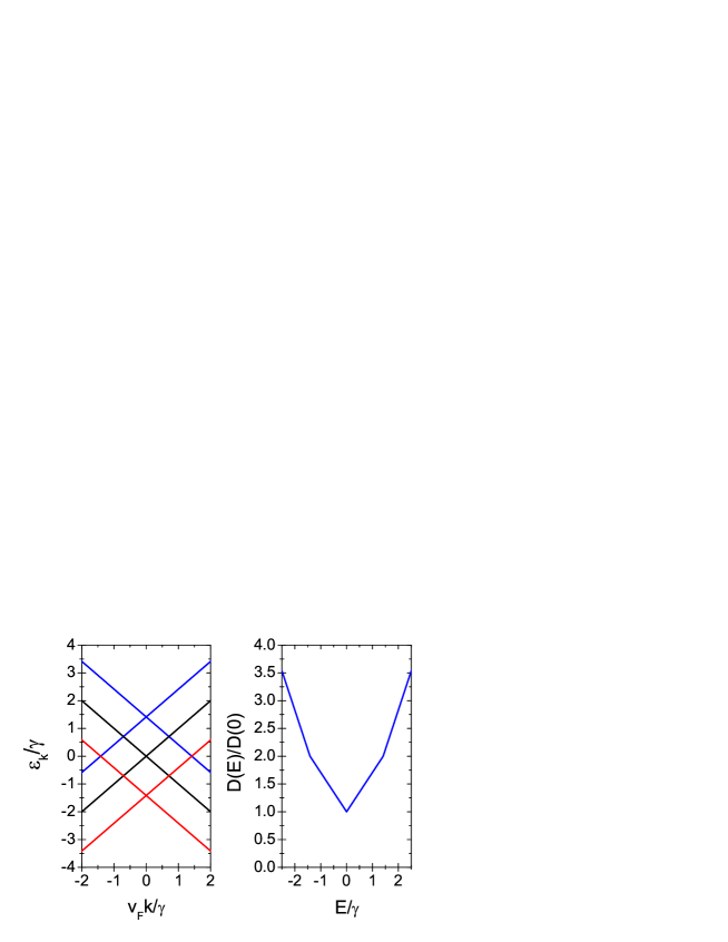
Figure 1: Left panel shows the low energy band structure of AAA-stacked TLG. Blue, black and red lines are correspond to different decoupled bands with band-indexes +, 0 and - respectively. Right panel shows the low energy density of states of AAA-stacked TLG normalized to its density of states at E=0, $D(0)=\sqrt{2}g\gamma/4\pi v_{F}^{2}$.

where multiple $g=4$ is due to spin and valley degeneracies. The low energy band structure and the density of states of AAA-stacked TLG have been shown in Fig. 1.

To consider screening properties of AAA-stacked TLG, we must calculate the static polarization. The total static polarization is the static limit of the total dynamic polarization, $\Pi(\mathbf{\mathbf{q}},\omega\rightarrow 0)$. The equivalent Matsubara function for the total dynamic polarization is given by

$$\Pi(\mathbf{q},i\omega_{n})=-\frac{1}{A}\int_{0}^{1/T}d\tau e^{i\omega_{n}\tau}\langle T_{\tau}\rho(\mathbf{q},\tau)\rho(-\mathbf{q},0)\rangle,$$ (45)

where $A$ is lattice area, $\omega_{n}$ are bosonic Matsubara frequencies and $T$ is the temperature. The retarded function for the static polarization is obtained from the Matsubara function by changing $i\omega_{n}$ to $\omega+i0^{+}$. By making use of the definition of the Green’s function, Eq. (45) becomes

$$\Pi(\mathbf{q},i\omega_{n})=-\frac{T}{A}\sum_{m\mathbf{k}}Tr[\hat{G}(\mathbf{k+q},i\nu_{m}+i\omega_{n})\hat{G}(\mathbf{k},i\nu_{m})].$$ (46)

We use the spectral function representation of the Matsubara Green’s function,

$$\hat{G}(\mathbf{k},i\omega_{n})=\int_{-\infty}^{+\infty}\frac{d\Omega}{2\pi}\frac{\hat{A}(\mathbf{k},\Omega)}{i\omega_{n}-\Omega},$$ (47)

and apply the Matsubara summation to obtain the following relation for the dynamic polarization

$$\Pi(\mathbf{q},i\omega_{n})=-\frac{g}{4A}[2\sum_{\mathbf{k},\lambda\lambda^{{}^{\prime}}}\frac{n_{\mathbf{k}}^{0\lambda}-n_{\mathbf{k+q}}^{0\lambda^{{}^{\prime}}}}{i\omega_{n}+\varepsilon_{\mathbf{k}}^{0\lambda}-\varepsilon_{\mathbf{k+q}}^{0\lambda^{{}^{\prime}}}}+\sum_{\mathbf{k},\lambda\lambda^{{}^{\prime}}s=\pm}\frac{n_{\mathbf{k}}^{s\lambda}-n_{\mathbf{k+q}}^{s\lambda^{{}^{\prime}}}}{i\omega_{n}+\varepsilon_{\mathbf{k}}^{s\lambda}-\varepsilon_{\mathbf{k+q}}^{s\lambda^{{}^{\prime}}}}]\times[1+\lambda\lambda^{{}^{\prime}}\cos\Delta\theta_{\mathbf{k}+\mathbf{q},\mathbf{k}}],$$ (48)

where $n_{\mathbf{k}}^{s\lambda}=1/(1+exp[(\varepsilon_{\mathbf{k}}^{s\lambda}-\mu)/T])$ is the Fermi-Dirac distribution function and $\Delta\theta_{\mathbf{k}+\mathbf{q},\mathbf{k}}=\theta_{\mathbf{k}+\mathbf{q}}-\theta_{\mathbf{k}}$.

One of the most attractive quantities, which can be calculated easily from the static polarization, is the screening of a charged impurity $Ze$. If the impurity is located at the center of the coordinate set, the intra-layer screened coulomb potential at distance $r$ from the impurity is $\phi(r)=\int qdq\phi(q)J_{0}(qr)/2\pi$, where $J_{0}(qr)$ is the Bessel function of the zeroth order and $\phi(q)$ is the Fourier transform of the screened coulomb potential. $\phi(q)$, at low energy excitations and within RPA, is given by $\phi(q)\approx 2\pi Ze^{2}/(\kappa q[1+(2\pi e^{2}/\kappa q)\Pi(q)])$ where $\Pi(q)$ is the total static polarization. In the next section we present our results for the static polarization and consider screening properties of AAA-stacked TLG.

3 Numerical Results

In this section, we consider screening properties of AAA-stacked TLG in several cases, in both undoped and doped cases and also in the presence of a bias voltage. In each case, first we calculate the static polarization. Then we study the Thomas-Fermi screening and the long-distance behavior of the screened coulomb potential. Our results are presented in the following subsections.

3.1 Undoped AAA-stacked TLG

In AAA-stacked TLG, similar to AA-stacked BLG and as Eq. (48) shows, only those transition contribute to the total static polarization that occur between bands with same s index. This is similar to what has been reported for the optical conductivity of AA-stacked BLG [17], where energy bands with different s index behave like decoupled bands. It is evident from Eq. (48) that the static polarization of AA-stacked TLG can be written as sum of four SLG-like terms for the static polarization, two terms with $\mu=0$ and two other terms with $\mu=\sqrt{2}\gamma$ and $\mu=-\sqrt{2}\gamma$ (all of them are weighted by $1/4$). Due to equality of later terms, we can write $\Pi(q)=\Pi_{SLG}^{\mu=0}(q)/2+\Pi_{SLG}^{\mu=\sqrt{2}\gamma}(q)/2$. At zero temperature, $\Pi(q)$ is given by (Appendix A)

$$\Pi(q)=\frac{1}{2}\frac{gq}{16v_{F}}+\frac{1}{2}\frac{\sqrt{2}g\gamma}{2\pi v_{F}^{2}},$$ (49)

for $q\leq 2\sqrt{2}\gamma/v_{F}$, and

$$\Pi(q)=\frac{1}{2}\frac{gq}{16v_{F}}+\frac{1}{2}[\frac{gq}{16v_{F}}+\frac{\sqrt{2}g\gamma}{2\pi v_{F}^{2}}(1-\frac{1}{2}\sqrt{1-(\frac{2\sqrt{2}\gamma}{v_{F}q})^{2}}-\frac{v_{F}q}{4\sqrt{2}\gamma}\sin^{-1}\frac{2\sqrt{2}\gamma}{v_{F}q})],$$ (50)

for $q>2\sqrt{2}\gamma/v_{F}$. It is evident that, for $q\leq\sqrt{2}\gamma$, the static polarization is a combination of a constant metallic-like polarization and an insulating-like polarization increasing linearly with $q$. This is a very different behavior from the ordinary two dimensional electron gas (2DEG) [35] and from other graphene-based materials [21, 22, 23, 24, 25, 26, 27, 28, 29, 30, 31, 32, 33, 34]. While for $q>\sqrt{2}\gamma$, that the interband transitions between bands with same s index dominate the intraband transitions, the static polarization of AAA-stacked TLG (similar to that in SLG [21, 23, 25]) increases linearly with $q$.

The static dielectric function is written as $\epsilon(q)=1+(2\pi e^{2}/\kappa q)\Pi(q)$ where $\kappa$ is the background dielectric constant. The linear part of the static polarization only leads to an enhancement of the effective background dielectric constant $\kappa^{\ast}=\kappa(1+\pi e^{2}g/16\kappa v_{F})$. While its constant metallic-like part (in the long-wavelength limit) gives rise to the Thomas-Fermi screening with $\epsilon(q)=1+q_{TF}/q$ where $q_{TF}=2\pi e^{2}D(0)/\kappa^{\ast}=\sqrt{2}g\gamma e^{2}/2\kappa^{\ast}v_{F}^{2}$ is the effective Thomas-Fermi screening wave vector. Note that the effective Thomas-Fermi screening wave vector in undoped AAA-stacked TLG, similar to that in the ordinary 2DEG [35] and AA-stacked BLG [29] (and contrary to that in SLG [21, 25]), is independent of the carrier concentration.

Another of interest quantity is the long-distance behavior of the screened coulomb potential from a charged impurity. This is determined by the long-wavelength behavior of the static polarization and its singularity. The long-wavelength behavior of the static polarization leads to a non-oscillatory term for the screened coulomb potential as [22, 26],

$$\phi(r)=\frac{Ze^{2}}{\kappa^{\ast}r}-\frac{\pi Ze^{2}q_{TF}}{2\kappa^{\ast}}[H_{0}(q_{TF}r)-Y_{0}(q_{TF}r)],$$ (51)

where $H_{0}$ and $Y_{0}$ are the Struve and the Bessel functions of the second kind and its asymptotic form at large distance is given by $Ze^{2}q_{TF}/[\kappa^{\ast}(q_{TF}r)^{3}]$. Furthermore, there is a discontinuity occurring in the second derivative of the static polarization ( as q approaches $2\sqrt{2}\gamma/v_{F}$ from above $d^{2}\Pi(q)/d^{2}q\leavevmode\nobreak\ \propto\leavevmode\nobreak\ 1/\sqrt{1-(2\sqrt{2}\gamma/qv_{F})^{2}}$), which leads to a Friedel-oscillation term for the screened coulomb potential. This term can be evaluated using a theorem of Lighthill [36], and whose asymptotic form is $k_{F}^{{}^{\prime}}cos(2k_{F}^{{}^{\prime}}r)/\kappa^{\ast}(k_{F}^{{}^{\prime}}r)^{3}$ where $k_{F}^{{}^{\prime}}=\sqrt{2}\gamma/v_{F}$(Appendix B). For AAA-stacked TLG, both terms are of same order in distance and must be kept to discuss the long-distance of the screened coulomb potential.

3.2 Effects of a bias voltage

Effects of a bias voltage can be considered via adding an electric potential matrix,

$$\widehat{V}=V\left(\begin{array}[]{ccc}\hat{1}&\hat{0}&\hat{0}\\ \hat{0}&\hat{0}&\hat{0}\\ \hat{0}&\hat{0}&-\hat{1}\\ \end{array}\right),$$ (55)

to the Hamiltonian matrix in Eq. (8), where $\hat{1}$ and $\hat{0}$ are $2\times 2$ unitary and zero matrix respectively. $2V$ is the difference between the applied electrical potential to the top and bottom layer. This leads to a new dispersion relation for AAA-stacked TLG as

$$\varepsilon_{V,\mathbf{k}}^{s\lambda}=s[(\sqrt{2}\gamma)^{2}+V^{2}]^{1/2}+\lambda v_{F}|\mathbf{k}|,$$ (56)

which indicates that effects of the bias voltage can be taken into account by a renormalization of the interlayer hopping energy of the unbiased AAA-stacked TLG, $\gamma$, to a new bias-voltage-dependent hopping energy, $\gamma^{{}^{\prime}}=[\gamma^{2}+V^{2}/2]^{1/2}$. Moreover, it is easy to show that Eq. (1) is also indefeasible for the dynamical polarization of the biased AAA-stacked TLG, but by replacing $\varepsilon_{\mathbf{k}}^{s\lambda}\rightarrow\varepsilon_{V,\mathbf{k}}^{s\lambda}$.

The static polarization of biased AAA-stacked TLG is obtained from Eqs. (49) and (50), by just substituting $\gamma\longleftrightarrow\gamma^{{}^{\prime}}$. Thus it, for $q<\sqrt{2}\gamma^{{}^{\prime}}/v_{F}$, is a combination of a constant metallic-like polarization and an insulating-like polarization increasing linearly with $q$. But it increases linearly with $q$ when $q<\sqrt{2}\gamma^{{}^{\prime}}/v_{F}$. The linear part of the static polarization (similar to the undoped case) gives rise to an enhancement of the effective background dielectric constant $\kappa^{\ast}=\kappa(1+\pi e^{2}g/16\kappa v_{F})$ which is not affected by the bias voltage. In the biased AAA-stacked TLG, the effective Thomas-Fermi screening wave vector depends on the applied bias voltage as $q_{TF}=\sqrt{2}ge^{2}[\gamma^{2}+V^{2}/2]^{1/2}/2\kappa^{\ast}v_{F}^{2}$, which indicates enhanced screening at high bias voltage. This also leads to a fast decayed screened coulomb potential as $\phi(r)\propto 1/[\gamma^{2}+V^{2}/2]$ at high bias voltage.

3.3 Effects of doping

Considering effects of doping on screening properties of AAA-stacked TLG is more attractive than the other cases. It is evident from Eq. (1) that, for $\mu>\sqrt{2}\gamma$, the static polarization of AAA-stacked is equal to that of a doped SLG lattice, a constant metallic polarization for $q\leq\mu/v_{F}$ and a linear in-q insulating polarization for $q>\mu/v_{F}$. Thus, when $\mu$ exceeds $\sqrt{2}\gamma$, screening properties of AAA-stacked TLG is similar to that of doped SLG [21, 22, 23, 24, 25, 26]. But when $\mu$ is less than $\sqrt{2}\gamma$, the static polarization of AAA-stacked TLG is given by $\Pi(q)=\Pi_{SLG}^{\mu}(q)/2+\Pi_{SLG}^{\sqrt{2}\gamma}(q)/2$ which is a constant metallic-like polarization (for $q\leq\mu/v_{F}$) and a linear in-q insulating-like one (when $q$ exceeds $\sqrt{2}\gamma/v_{F}$), while, for $\mu/v_{F}<q\leq\sqrt{2}\gamma/v_{F}$, it is a combination of the constant metallic-like and the linear in-q insulating-like polarization. This is in contrast to what has been reported for the ordinary 2DEG [21] and for the other graphene-based materials [21, 22, 23, 24, 25, 26, 27, 33].

The long-wavelength limit of the static dielectric function is given by $\epsilon(q)\approx 1+q_{TF}/q$, where $q_{TF}=2\pi e^{2}D(0)/\kappa=ge^{2}(\mu+\sqrt{2}\gamma)/2\kappa v_{F}^{2}$. Note that the Thomas-Fermi screening wave vector depends on doping and the interlayer hopping energy. This indicates that screening properties of AAA-stacked TLG neither are only determined by doping (similar to that in SLG) nor are only determined by the interlayer hopping energy (similar to that in AA-stacked BLG). It is evident that, in addition to doping (in SLG ) and the interlayer hopping energy (in AA-stacked BLG), screening properties also depends on the Fermi velocity, $v_{F}$.

In the doped AAA-stacked TLG, the screened Coulomb potential has another Freidel-oscillation term coming from the discontinuity of $d^{2}\Pi(q)/d^{2}q$ at $q=k_{F}=\mu/v_{F}$. This term at large distance decays as $k_{F}\cos(2k_{F}r)/\kappa(k_{F}r)^{3}$ and it can be tuned by doping. While the other Friedel-oscillation term, $k_{F}^{{}^{\prime}}\cos(2k_{F}^{{}^{\prime}})/\kappa(k_{F}^{{}^{\prime}}r)^{3}$, only depends on the interlayer hopping energy and it is not affected by doping. The non-oscillatory part of the screened coulomb potential which decays at large distances as $eq_{TF}/[\kappa(q_{TF}r)^{3}]$, due to partial dependence of $eq_{TF}$ on $\mu$, can be suppressed by doping partially.

4 Summary and conclusions

In summary, we studied screening properties of a AAA-stacked TLG lattice within RPA in all undoped, doped and biased regimes. We found that in undoped case, the static polarization of AAA-stacked TLG is a combination of a constant metallic-like and an insulating-like polarization, leading to an enhancement of the effective background dielectric constant along a Thomas-Fermi screening with the Thomas-Fermi wave vector which, similar to that in ordinary 2DEG and undoped AA-stacked BLG, is independent of the carrier concentrations. We also discussed the long-distance behavior of the screened Coulomb potential determined by two terms, a non-oscillatory term coming from the long-wavelength limit of the static polarization and a Freidel-oscillation term coming from the discontinuity in the second derivative of the polarization, whose asymptotic forms at large distances are $1/r^{3}$ and $cos(2k_{F}^{{}^{\prime}}r)/r^{3}$ respectively.

Moreover, we studied effects of a bias voltage and showed that it can be taken into account by a renormalization of the interlayer hopping energy to a new value, $\gamma\rightarrow\sqrt{\gamma^{2}+V^{2}/2}$. We showed that screening properties of biased AAA-stacked TLG, e.g., the Thomas-Fermi wave vector and the long-distance behavior of the screened coulomb potential, can be tuned by the bias voltage.

At the final subsection, we considered screening properties of doped AAA-stacked TLG. We showed that when $\mu$ exceeds $\sqrt{2}\gamma$, screening properties of doped AAA-stacked TLG is similar to that of doped SLG. But for doped AAA-satcked TLG with $\mu\leq\sqrt{2}\gamma$, screening properties are dependent on the inerlayer hopping energy and doping, in contrast to that in SLG only depending on doping and to that in AA-stacked BLG only depending on the inerlayer hopping energy.

5 Appendix A: Calculating $\Pi(q,0)$

In the undoped case, $\Pi(q,\omega)$ can be written as

$$\Pi(q,\omega)=\frac{1}{4}(2\Pi^{ud}(q,\omega)+\Pi^{pd}(q,\omega)+\Pi^{hd}(q,\omega)).\leavevmode\nobreak\ \leavevmode\nobreak\ \leavevmode\nobreak\ \leavevmode\nobreak\ \leavevmode\nobreak\ \leavevmode\nobreak\ \leavevmode\nobreak\ \leavevmode\nobreak\ \leavevmode\nobreak\ \leavevmode\nobreak\ \leavevmode\nobreak\ \leavevmode\nobreak\ \leavevmode\nobreak\ \leavevmode\nobreak\ \leavevmode\nobreak\ \leavevmode\nobreak\ \leavevmode\nobreak\ \leavevmode\nobreak\ \leavevmode\nobreak\ \leavevmode\nobreak\ \leavevmode\nobreak\ \leavevmode\nobreak\ \leavevmode\nobreak\ \leavevmode\nobreak\ \leavevmode\nobreak\ \leavevmode\nobreak\ \leavevmode\nobreak\ \leavevmode\nobreak\ \leavevmode\nobreak\ \leavevmode\nobreak\ \leavevmode\nobreak\ (A.1)$$

The imaginary part of $\Pi^{ud}(q,\omega)$ is given by

$$Im\Pi^{ud}(q,\omega)=g\int_{0}^{\infty}\frac{kdk}{8\pi}\int_{0}^{2\pi}d\varphi\frac{|\mathbf{k+q}|-k-q\cos\varphi}{|\mathbf{k+q}|}\sum_{\lambda=\pm}\lambda\delta(\omega+\lambda v_{F}(k+|\mathbf{k+q}|)).\leavevmode\nobreak\ \leavevmode\nobreak\ \leavevmode\nobreak\ \leavevmode\nobreak\ (A.2)$$

The $\varphi$-integration yields

$$Im\Pi^{ud}(q,\omega)=g\int_{\frac{\frac{\omega}{v_{F}}-q}{2}}^{\frac{\frac{\omega}{v_{F}}+q}{2}}\frac{dk}{4\pi}\sqrt{\frac{(\frac{\omega}{v_{F}}-2k)^{2}-q^{2}}{(\frac{\omega}{v_{F}})^{2}-q^{2}}},\leavevmode\nobreak\ \leavevmode\nobreak\ \leavevmode\nobreak\ \leavevmode\nobreak\ \leavevmode\nobreak\ \leavevmode\nobreak\ \leavevmode\nobreak\ \leavevmode\nobreak\ \leavevmode\nobreak\ \leavevmode\nobreak\ \leavevmode\nobreak\ \leavevmode\nobreak\ \leavevmode\nobreak\ \leavevmode\nobreak\ \leavevmode\nobreak\ \leavevmode\nobreak\ \leavevmode\nobreak\ \leavevmode\nobreak\ \leavevmode\nobreak\ \leavevmode\nobreak\ \leavevmode\nobreak\ \leavevmode\nobreak\ \leavevmode\nobreak\ (A.3)$$

which after integration over $k$ becomes

$$Im\Pi^{ud}(q,\omega)=\frac{gq^{2}}{16v_{F}\sqrt{(\omega/v_{F})^{2}-q^{2}}}.\leavevmode\nobreak\ \leavevmode\nobreak\ \leavevmode\nobreak\ \leavevmode\nobreak\ \leavevmode\nobreak\ \leavevmode\nobreak\ \leavevmode\nobreak\ \leavevmode\nobreak\ \leavevmode\nobreak\ \leavevmode\nobreak\ \leavevmode\nobreak\ \leavevmode\nobreak\ \leavevmode\nobreak\ \leavevmode\nobreak\ \leavevmode\nobreak\ \leavevmode\nobreak\ \leavevmode\nobreak\ \leavevmode\nobreak\ \leavevmode\nobreak\ \leavevmode\nobreak\ \leavevmode\nobreak\ \leavevmode\nobreak\ \leavevmode\nobreak\ \leavevmode\nobreak\ (A.4)$$

Using the Kramers-Kornig relation, the real part of $\Pi^{ud}(q,\omega)$,

$$Re\Pi^{ud}(q,\omega)=\frac{gq^{2}}{16v_{F}\sqrt{q^{2}-(\omega/v_{F})^{2}}},\leavevmode\nobreak\ \leavevmode\nobreak\ \leavevmode\nobreak\ \leavevmode\nobreak\ \leavevmode\nobreak\ \leavevmode\nobreak\ \leavevmode\nobreak\ \leavevmode\nobreak\ \leavevmode\nobreak\ \leavevmode\nobreak\ \leavevmode\nobreak\ \leavevmode\nobreak\ \leavevmode\nobreak\ \leavevmode\nobreak\ \leavevmode\nobreak\ \leavevmode\nobreak\ \leavevmode\nobreak\ \leavevmode\nobreak\ \leavevmode\nobreak\ \leavevmode\nobreak\ \leavevmode\nobreak\ \leavevmode\nobreak\ \leavevmode\nobreak\ \leavevmode\nobreak\ (A.5)$$

is obtained, indicating $\Pi^{ud}(q)=\Pi_{SLG}^{\mu=0}(q)=\frac{gq}{16v_{F}}$ [21, 22, 25]. The particle-doped part of $\Pi(q,\omega)$ can be written as

$$\Pi^{pd}(q)=\frac{gq}{16v_{F}}+g\int_{0}^{\infty}\frac{dk}{2\pi^{2}v_{F}}\theta(\sqrt{2}\gamma-v_{F}k)[\int_{0}^{\pi}d\varphi(1-\frac{1-(2k/q)^{2}}{1+2(k/q)\cos\varphi}].\leavevmode\nobreak\ \leavevmode\nobreak\ \leavevmode\nobreak\ \leavevmode\nobreak\ \leavevmode\nobreak\ \leavevmode\nobreak\ \leavevmode\nobreak\ \leavevmode\nobreak\ \leavevmode\nobreak\ \leavevmode\nobreak\ \leavevmode\nobreak\ \leavevmode\nobreak\ \leavevmode\nobreak\ \leavevmode\nobreak\ \leavevmode\nobreak\ \leavevmode\nobreak\ \leavevmode\nobreak\ (A.6)$$

The $\varphi$-integration yields

$$\Pi^{pd}(q)= \frac{gq}{16v_{F}}+\frac{g\sqrt{2}\gamma}{2\pi v_{F}^{2}}-\frac{g}{2\pi^{2}v_{F}}[\int_{0}^{q/2}dk(\theta(\sqrt{2}\gamma-v_{F}k)[2uv\tan^{-1}(\frac{u}{v}\tan\frac{\varphi}{2})|_{\varphi=0}^{\varphi=\pi}])+$$

$$\int_{q/2}^{\infty}dk(\theta(\sqrt{2}\gamma-v_{F}k)[2uw\ln|\frac{u\cos\frac{\varphi}{2}+w\sin\frac{\varphi}{2}}{u\cos\frac{\varphi}{2}-w\sin\frac{\varphi}{2}}|_{\varphi=0}^{\varphi=\pi}])],\leavevmode\nobreak\ \leavevmode\nobreak\ \leavevmode\nobreak\ \leavevmode\nobreak\ \leavevmode\nobreak\ \leavevmode\nobreak\ \leavevmode\nobreak\ \leavevmode\nobreak\ \leavevmode\nobreak\ \leavevmode\nobreak\ \leavevmode\nobreak\ \leavevmode\nobreak\ \leavevmode\nobreak\ \leavevmode\nobreak\ \leavevmode\nobreak\ \leavevmode\nobreak\ \leavevmode\nobreak\ \leavevmode\nobreak\ \leavevmode\nobreak\ \leavevmode\nobreak\ \leavevmode\nobreak\ \leavevmode\nobreak\ \leavevmode\nobreak\ \leavevmode\nobreak\ (A.7)$$

where $u=\sqrt{1+2k/q}$ and $v=\sqrt{1-2k/q}=iw$. After integrating over $k$ we have

$$\Pi^{pd}(q)=\frac{gq}{16v_{F}}+\frac{g\sqrt{2}\gamma}{2\pi v_{F}^{2}}-\frac{gq}{16v_{F}},\leavevmode\nobreak\ \leavevmode\nobreak\ \leavevmode\nobreak\ \leavevmode\nobreak\ \leavevmode\nobreak\ \leavevmode\nobreak\ \leavevmode\nobreak\ \leavevmode\nobreak\ \leavevmode\nobreak\ \leavevmode\nobreak\ \leavevmode\nobreak\ \leavevmode\nobreak\ \leavevmode\nobreak\ \leavevmode\nobreak\ \leavevmode\nobreak\ \leavevmode\nobreak\ \leavevmode\nobreak\ \leavevmode\nobreak\ \leavevmode\nobreak\ \leavevmode\nobreak\ \leavevmode\nobreak\ \leavevmode\nobreak\ \leavevmode\nobreak\ \leavevmode\nobreak\ (A.8)$$

for $q<2\sqrt{2}\gamma/v_{F}$, and

$$\Pi^{pd}(q)=\frac{gq}{16v_{F}}+\frac{g\sqrt{2}\gamma}{2\pi v_{F}^{2}}-\frac{1}{2}\frac{g\sqrt{2}\gamma}{2\pi v_{F}^{2}}[\sqrt{1-(\frac{2\sqrt{2}\gamma}{v_{F}q})^{2}}+\frac{v_{F}q}{2\sqrt{2}\gamma}\sin^{-1}(\frac{2\sqrt{2}\gamma}{v_{F}q})],\leavevmode\nobreak\ \leavevmode\nobreak\ \leavevmode\nobreak\ \leavevmode\nobreak\ \leavevmode\nobreak\ \leavevmode\nobreak\ \leavevmode\nobreak\ \leavevmode\nobreak\ \leavevmode\nobreak\ (A.9)$$

for $q>2\sqrt{2}\gamma/v_{F}$. This is equal to $\Pi_{SLG}^{\mu=\sqrt{2}\gamma}(q)$ [25, 25]. The hole-doped part of $\Pi(q,\omega)$ is

$$\Pi^{hd}(q)=\frac{1}{A}\sum_{\mathbf{k}}[\frac{1+\cos\Delta\theta_{\mathbf{k}+\mathbf{q},\mathbf{k}}}{v_{F}(|\mathbf{k}|-|\mathbf{k+q}|)}(n_{\mathbf{k}}^{+-}-n_{\mathbf{k+q}}^{+-})+\frac{1-\cos\Delta\theta_{\mathbf{k}+\mathbf{q},\mathbf{k}}}{v_{F}(|\mathbf{k}|+|\mathbf{k+q}|)}(n_{\mathbf{k}}^{+-}+n_{\mathbf{k+q}}^{+-})],\leavevmode\nobreak\ \leavevmode\nobreak\ \leavevmode\nobreak\ (A.10)$$

where $n_{\mathbf{k}}^{+-}=1-\theta(\sqrt{2}\gamma-v_{F}|\mathbf{k}|)$. After substituting these terms into eq. (A.10), we get

$$\Pi^{hd}(q)=\Pi^{ud}(q)-\frac{g}{A}\sum_{\mathbf{k}}\theta(\sqrt{2}\gamma-v_{F}|\mathbf{k}|)[\sum_{\lambda=\pm}\frac{1-\lambda\cos\Delta\theta_{\mathbf{k}+\mathbf{q},\mathbf{k}}}{v_{F}(|\mathbf{k}|+\lambda|\mathbf{k+q}|)}],\leavevmode\nobreak\ \leavevmode\nobreak\ \leavevmode\nobreak\ \leavevmode\nobreak\ \leavevmode\nobreak\ \leavevmode\nobreak\ \leavevmode\nobreak\ \leavevmode\nobreak\ \leavevmode\nobreak\ \leavevmode\nobreak\ \leavevmode\nobreak\ \leavevmode\nobreak\ \leavevmode\nobreak\ \leavevmode\nobreak\ \leavevmode\nobreak\ (A.11)$$

which is equal to $\Pi^{pd}(q)$. The static polarization of biased AAA-stacked TLG can be obtained easily as it has been calculated in the undoped case just by substituting $\gamma\longleftrightarrow\gamma^{{}^{\prime}}$. Also the static polarization of doped AAA-stacked TLG is calculated similar to $\Pi^{pd}(q)$(or $\Pi^{hd}(q)$) of the static polarization in the undoped case.

6 Appendix B: Friedel oscillations

The Friedel oscillation, which comes from singularities of the static dielectric function, can be calculated by making use of a theorem of Lighthill [36]. According to this theorem, the asymptotic expression for the Fourier transform of function $f(x)$, which has a finite number of singularities $x=x_{1},x_{2},...,x_{M}$, is given by

$$g(y)=\sum_{m=1}^{M}G_{m}(y)+o(|y|^{-N})\leavevmode\nobreak\ \leavevmode\nobreak\ as\leavevmode\nobreak\ \leavevmode\nobreak\ |y|\rightarrow\infty,\leavevmode\nobreak\ \leavevmode\nobreak\ \leavevmode\nobreak\ \leavevmode\nobreak\ \leavevmode\nobreak\ \leavevmode\nobreak\ \leavevmode\nobreak\ \leavevmode\nobreak\ \leavevmode\nobreak\ \leavevmode\nobreak\ \leavevmode\nobreak\ \leavevmode\nobreak\ \leavevmode\nobreak\ \leavevmode\nobreak\ \leavevmode\nobreak\ \leavevmode\nobreak\ \leavevmode\nobreak\ \leavevmode\nobreak\ \leavevmode\nobreak\ \leavevmode\nobreak\ \leavevmode\nobreak\ \leavevmode\nobreak\ \leavevmode\nobreak\ (B.1)$$

where $g(y)$ is the Fourier transform of $f(x)$ and $G_{m}(y)$ are the Fourier transform of $F_{m}(x)$ which make Nth derivative of $f(x)-F_{m}(x)$ absolutely integrable in an interval including $x_{m}$.

To obtain the asymptotic expression of the Friedel oscillation we must use the asymptotic form of the zeroth-order of the Bessel function. Therefore, we have

$$\phi(r)\simeq Ze^{2}\frac{\sqrt{k_{F}}}{\sqrt{\pi r}}\int_{0}^{\infty}\frac{\cos(k_{F}rx)+\sin(k_{F}rx)}{x+\frac{2\pi e^{2}}{k_{F}}\Pi(x)}\sqrt{x}dx,\leavevmode\nobreak\ \leavevmode\nobreak\ \leavevmode\nobreak\ \leavevmode\nobreak\ \leavevmode\nobreak\ \leavevmode\nobreak\ \leavevmode\nobreak\ \leavevmode\nobreak\ \leavevmode\nobreak\ \leavevmode\nobreak\ \leavevmode\nobreak\ \leavevmode\nobreak\ \leavevmode\nobreak\ \leavevmode\nobreak\ (B.2)$$

where $k_{F}=\sqrt{2}\gamma/v_{F}$, $x=q/k_{F}$.

By making use of the theorem and the asymptotic behavior of the Fourier transform of the function $\theta(x-2)\sqrt{|x-2|^{3}}$ which is

$$g(y)\simeq\frac{3\sqrt{\pi}}{4(2\pi|y|)^{5/2}}e^{-i(2y+5\pi/4)}\leavevmode\nobreak\ ,\leavevmode\nobreak\ \leavevmode\nobreak\ \leavevmode\nobreak\ \leavevmode\nobreak\ \leavevmode\nobreak\ \leavevmode\nobreak\ \leavevmode\nobreak\ \leavevmode\nobreak\ \leavevmode\nobreak\ \leavevmode\nobreak\ \leavevmode\nobreak\ \leavevmode\nobreak\ \leavevmode\nobreak\ \leavevmode\nobreak\ \leavevmode\nobreak\ \leavevmode\nobreak\ \leavevmode\nobreak\ \leavevmode\nobreak\ \leavevmode\nobreak\ \leavevmode\nobreak\ \leavevmode\nobreak\ \leavevmode\nobreak\ \leavevmode\nobreak\ \leavevmode\nobreak\ \leavevmode\nobreak\ \leavevmode\nobreak\ \leavevmode\nobreak\ \leavevmode\nobreak\ (B.3)$$

we obtain the asymptotic form of the Friedel oscillation,

$$\phi(r)\simeq-\frac{3Ze^{2}}{4\kappa^{\ast}}\frac{k_{F}^{{}^{\prime}}\alpha}{(1+\pi\alpha)^{2}}\frac{\cos(2k_{F}^{{}^{\prime}}r)}{(k_{F}^{{}^{\prime}}r)^{3}}\leavevmode\nobreak\ ,\leavevmode\nobreak\ \leavevmode\nobreak\ \leavevmode\nobreak\ \leavevmode\nobreak\ \leavevmode\nobreak\ \leavevmode\nobreak\ \leavevmode\nobreak\ \leavevmode\nobreak\ \leavevmode\nobreak\ \leavevmode\nobreak\ \leavevmode\nobreak\ \leavevmode\nobreak\ \leavevmode\nobreak\ \leavevmode\nobreak\ \leavevmode\nobreak\ \leavevmode\nobreak\ \leavevmode\nobreak\ \leavevmode\nobreak\ \leavevmode\nobreak\ \leavevmode\nobreak\ \leavevmode\nobreak\ \leavevmode\nobreak\ \leavevmode\nobreak\ \leavevmode\nobreak\ \leavevmode\nobreak\ (B.4)$$

where $k_{F}^{{}^{\prime}}=\sqrt{2}\gamma/v_{F}$ and $\alpha=e^{2}/\kappa^{\ast}v_{F}$. The Friedel oscillation coming from the discontinuity $d^{2}\Pi(q)/d^{2}q$ at $\sqrt{2}[\gamma^{2}+V^{2}/2]^{1/2}/v_{F}$(in the biased case) and $q=\mu/v_{F}$(in the doped case) are obtained completely similar to that in the undoped case.

References

- [1] A. H. Castro Neto, F. Guinea, N. M. R. Peres, K. S. Novoselov and A. K. Geim, Rev. Mod. Phys. 81 (2009) 109-162.
- [2] N. M. R. Peres, Rev. Mod. Phys. 82 (2010) 2673-2700.
- [3] B. Partoens, F. M. Peeters, Phys. Rev. B 75 (2007) 193402-193404.
- [4] M. Koshino, T. Ando, Phys. Rev. B 77 (2008) 115313-115323.
- [5] J. Nilsson, A. H. Castro Neto, F. Guinea, N. M. R. Peres, Phys. Rev. B 78 (2008) 045405-045438.
- [6] A. A. Avetisyan, B. Partoens, F. M. Peeters, Phys. Rev. B 80 (2009) 195401-195411.
- [7] M. Koshino, Phys. Rev. B 81 (2010) 125304-125310.
- [8] S. Das Sarma, S. Adam, E. H. Hwang, E. Rossi, Rev. Mod. Phys. 83 (2011) 407-470.
- [9] J. Jung, F. Zhang, Z. Qiao, A. H. MacDonald, Phys. Rev. B 84 (2011) 075418-075422.
- [10] P. L. De Andres, F. Guinea, M. I. Katsnelson, Phys. Rev. B 86 (2012) 144103-144107.
- [11] W. A. Munoz, L. Covaci, F. M. Peeters, Phys. Rev. B 88 (2013) 214502-214506.
- [12] Z. Liu, K. Suenaga, P. J. Harris, S. Iijima, Phys. Rev. Lett. 102 (2009) 015501-015504.
- [13] J. Borysiuk, J. Soltys, J. Piechota, Journal of Applied Physics 109 (2011) 093523-093527.
- [14] T. Ando, Journal of Physics: Conference Series 302 (2011) 012015-012027.
- [15] Y. -F. Hsu, G. -Y. Guo, Phys. Rev. B 82 (2011) 165404-165411.
- [16] E. Prada, P. San-Jose, L. Brey, H. Fertig, Solid State Commun. 151 (2011) 1065-1070.
- [17] C. J. Tabert, E. J. Nicol, Phys. Rev. B 84 (2012) 075439-075450.
- [18] C.-W. Chiu, F.-L. Shyu, M.-F. Lin, G. Gumbs, O. Roslyak, arXiv:1208.3356. 2012.
- [19] L. Brey, H. A. Fertig, Phys. Rev. B 87 (2013) 115411-115418.
- [20] Y. Mohammadi, R. Moradian, Physica B 442 (2014) 66-69.
- [21] T. Ando, J. Phys. Soc. Japan 75 (2006) 074716-074722.
- [22] M. I. Katsnelson, Phys. Rev. B 74 (2006) 201401-201403.
- [23] B. Wunsch, T. Stauber, F. Sols, F. Guinea, New. J. Phys. 8 (2006) 318-332.
- [24] V. V. Cheianov, V. I. Fal’ko, Phys. Rev. Lett. 97 (2006) 226801-226804.
- [25] E. H. Hwang, S. Das Sarma, Phys. Rev. B 75 (2007) 205418-205423.
- [26] E. H. Hwang, S. Das Sarma, Phys. Rev. Lett. 101 (2008) 156802-156805.
- [27] O. V. Gamayun, Phys. Rev. B 84 (2011) 085112-085121.
- [28] C. Triola, E. Rossi, Phys. Rev. B 86 (2012) 161408-161412.
- [29] R. Roldan, L. Brey, Phys. Rev. B 88 (2013) 115420-115426.
- [30] T. Ohta, A. Bostwick, J. L. McChesney, T. Seyller, K. Horn, E. Rotenberg, Phys. Rev. Lett. 98 (2007) 206802-206805.
- [31] D. Sun, C. Divin, C. Berger, W. A. de Heer, P. N. First, T. B. Norris, Phys. Rev. Lett. 104 (2010) 136802-136805.
- [32] M. A. Kuroda, J. Tersoff, G. J. Martyna, Phys. Rev. Lett. 106 (2011) 116804-116807.
- [33] H. Min, E. H. Hwang, S. Das Sarma, Phys. Rev. B(R) 86 (2012) 081402-081406.
- [34] R. van Gelderen, R. Olsen, C. M. Smith, Phys. Rev. B 88 (2013) 115414-115423.
- [35] T. Ando, A. B. Fowler, F. Stern, Rev. Mod. Phys. 54 (1982) 437-672.
- [36] M. J. Lighthill, Introduction to Fourier Analysis and Generalised Functions, Cambridge University Press, Cambridge, 1958, p.52.