Cooling mechanical resonators to quantum ground state from room temperature

Abstract

Ground-state cooling of mesoscopic mechanical resonators is a fundamental requirement for test of quantum theory and for implementation of quantum information. We analyze the cavity optomechanical cooling limits in the intermediate coupling regime, where the light-enhanced optomechanical coupling strength is comparable with the cavity decay rate. It is found that in this regime the cooling breaks through the limits in both the strong and weak coupling regimes. The lowest cooling limit is derived analytically at the optimal conditions of cavity decay rate and coupling strength. In essence, cooling to the quantum ground state requires $Q_{\mathrm{m}}>2.4n_{\mathrm{th}}$, with $Q_{\mathrm{m}}$ being the mechanical quality factor and $n_{\mathrm{th}}$ being the thermal phonon number. Remarkably, ground-state cooling is achievable starting from room temperature, when mechanical $Q$-frequency product $Q_{\mathrm{m}}{\nu>1.5}\times 10^{13}$, and both of the cavity decay rate and the coupling strength exceed the thermal decoherence rate. Our study provides a general framework for optimizing the backaction cooling of mesoscopic mechanical resonators.

Cavity optomechanics RevSci08 ; RevPhy09 ; RevRMP13 ; RevCPB13 ; Pierre provides an important platform for manipulation of mesoscopic mechanical resonators in the quantum regime. A prominent example is motional ground-state cooling, which reduces the thermal noise of the mechanical resonator all the way to the quantum ground state GSNat11 ; GSNat11-2 . This offers as the first crucial step for most applications such as the exploration of quantum-classical boundary superPRL11 ; superPRL12 ; superPRA13zqyin and quantum information processing qcPRL03 ; NetworkPRL10 ; QIPPRL12 . Recently cooling of mechanical resonators has been demonstrated using various approaches including pure cryogenic cooling GSNat10 , feedback cooling FBCooPRL98 ; FBCooPRL99 ; FBCooNat06 ; FBCooPRL07 ; FBCooPRL07-2 and cavity-assisted backaction cooling CooNat06 ; CooNat06-2 ; CooPRL06 ; CooNatPhys08 ; CooNatPhys09-1 ; CooNatPhys09-2 ; CooNatPhys09-3 ; CooNat10 ; GSNat11 ; GSNat11-2 ; CooPRA11 , along with many theoretical and experimental efforts on novel cooling schemes, such as cooling with dissipative coupling DCPRL09 ; LiPRL2009 ; DCPRL11 ; DCPRA13 ; myyanPRA13 , quadratic coupling quadCooPRA10 , single-photon strong coupling SSCCooPRA12 , hybrid systems Atom09PRA ; AtomPRA13 , laser pulse modulations PulPNAS11 ; PulPRA11-1 ; PulPRA11-2 ; PulPRL11 ; PulPRL12 and dissipation modulations ycliuDC13 . It is theoretically shown that ground-state cooling is possible in the resolved sideband regime PRL07-1 ; PRL07-2 ; PRA08 , where the mechanical resonance frequency is greater than the decay rate of the optical cavity, indicating the resolved mechanical sideband from cavity mode spectrum. These analyses are in the weak coupling regime, where the light-enhanced optomechanical coupling strength ${G}$ is weak compared with the cavity decay rate ${\kappa}$, and thus the coupling is regarded as a perturbation to the optical field. Within this regime a larger coupling strength is better since the net cooling rate (optical damping rate) scales as ${\Gamma}_{\mathrm{wk}}={4G}^{2}/\kappa$. On the other hand, when ${G\gg\kappa}$, the system is in the strong coupling regime SCPRL08 ; SCNJP08 ; SCNat09 ; SCNat11 ; SCNat12 ; SCNat13 ; ycliuDC13 , where normal-mode splitting occurs and the phonon occupancy exhibits Rabi-like oscillation with reversible energy exchange between optical and mechanical modes. Then the cooling rate saturates with the maximum value of ${\Gamma}_{\mathrm{str}}={\kappa}$, and thus a larger cavity decay rate ${\kappa}$ is better. However, in this case, a large ${\kappa}$ in turn makes the system away from the strong coupling regime. As a result, the optimal cooling is expected for the intermediate coupling regime, where the coupling strength ${G}$ is comparable with the cavity decay rate ${\kappa}$.

In the weak coupling regime, the perturbative approach PRL07-1 ; PRL07-2 is widely adopt. In the intermediate and strong coupling regimes, however, the perturbative approach fails since the optomechanical coupling can no longer be considered as a perturbation. One way to overcome this problem is to employ the covariance approach, where all the mean values of the second-order moments are computed with the linearized optomechanical interaction SCNJP08 ; ycliuDC13 . In this paper, we use this non-perturbative approach to analyze the optimal cooling limits in the full parameter range and derive the optimal parameters, including laser detuning, cavity decay rate and optomechanical coupling strength. We then find that the optimal cooling is reached with ${G}\sim 0.6\kappa$, which is in the intermediate coupling regime. Finally we show the unique advantage of cooling in this regime, where room-temperature ground-state cooling is achievable for mechanical $Q$-frequency product $Q_{\mathrm{m}}{\nu>1.5}\times 10^{13}$, which is within reach for current experimental conditions highQPRL14 .

We consider the general model of an optomechanical system, as shown in the set of Fig. 1. A mechanical mode interacts with an optical resonance mode which is driven by a coherent laser. The system Hamiltonian reads $H={{\omega}_{\mathrm{c}}a^{{\dagger}}a}+{\omega_{\mathrm{m}}b^{{\dagger}}b+ga^{{\dagger}}a{(b+b^{{\dagger}})+({\Omega e}}}^{-i\omega t}{a^{{\dagger}}+\Omega}^{\ast}{{{e}}}^{i\omega t}{a)}$. Here ${\omega}_{\mathrm{c}}$ (${\omega_{\mathrm{m}}}$) is the angular resonance frequency of the optical mode $a$ (mechanical mode $b$); the third term describes the optomechanical interaction LawPRA95 , with $g$ being the single-photon coupling rate; the last term describes the driving of the input laser with driving strength ${{\Omega}}$ and frequency $\omega$. The coherent driving shifts the optical states and thereby shifts the mechanical states via the optical force. Thus the operators are rewritten as ${a\rightarrow\alpha+a}_{1}$ and $b\rightarrow\beta+b_{1}$, where ${\alpha}$ ($\beta$) represents the steady state value of the optical (mechanical) mode, and ${a}_{1}$ ($b_{1}$) stands for the corresponding fluctuation operator. For strong intracavity field $\left|{\alpha}\right|\gg 1$, the Hamiltonian is approximated as quadratic type given by $H_{L}=-\Delta^{\prime}{a_{1}^{{\dagger}}a}_{1}+{\omega_{\mathrm{m}}{b_{1}^{{\dagger}}b}_{1}+G(a_{1}^{{\dagger}}+a_{1})(b_{1}+b_{1}^{{\dagger}}})$, where $G=\left|{\alpha}\right|{g}$ describes the light-enhanced optomechanical coupling strength and ${\Delta}^{\prime}=\omega-{{\omega}_{\mathrm{c}}}+2{G}^{2}/{\omega_{\mathrm{m}}}$ denotes the optomechanical-coupling modified detuning. In the above derivation we have absorbed the phase factor of ${\alpha}$ into the operator $a$.

The system evolution is governed by master equation described by $\dot{\rho}=i[\rho,H_{L}]+\kappa\mathcal{D}[{a}_{1}]\rho+\gamma(n_{\mathrm{th}}+1)\mathcal{D}[{{b}_{1}}]\rho+\gamma n_{\mathrm{th}}\mathcal{D}[{{b_{1}^{{\dagger}}}}]\rho$. Here $\mathcal{D}[\hat{o}]\rho=\hat{o}\rho\hat{o}^{{\dagger}}-{({\hat{o}^{{\dagger}}\hat{o}\rho+\rho\hat{o}^{{\dagger}}\hat{o})/2}}$ (${{\hat{o}=a}}_{1}$, ${{b}_{1}}$, ${{b_{1}^{{\dagger}}}}$) denotes the Lindblad dissipators; $\kappa$ ($\gamma$) represents the dissipation rate of the optical cavity (mechanical) mode; $n_{\mathrm{th}}=1/(e^{\hbar{\omega_{\mathrm{m}}/k}_{\mathrm{B}}T}-1)$ corresponds to the bath thermal phonon number at the environmental temperature $T$. Using the master equation, the mean phonon number $\bar{N}_{b}=\langle{b_{1}^{{\dagger}}b}_{1}\rangle=\mathrm{Tr}(\rho{b_{1}^{{\dagger}}b}_{1})$ can be determined by a linear system of ordinary differential equations involving all the second-order moments SCNJP08 ; ycliuDC13 ; ycliuSC14 , i. e., $\partial_{t}\langle\hat{o}_{i}\hat{o}_{j}\rangle=\mathrm{Tr}(\dot{\rho}\hat{o}_{i}\hat{o}_{j})=\sum_{k,l}\eta_{k,l}\langle\hat{o}_{k}\hat{o}_{l}\rangle$, where $\hat{o}_{i}$, $\hat{o}_{j}$, $\hat{o}_{k}$ and $\hat{o}_{l}$ are one of the operators ${{a}}_{1}$, ${{b}_{1}}$, ${{a_{1}^{{\dagger}}}}$ and ${{b_{1}^{{\dagger}}}}$. Initially, the mean phonon number is equal to the bath thermal phonon number, i. e., $\bar{N}_{b}(t=0)=n_{\mathrm{th}}$, and other second-order moments are zero.

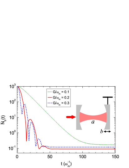
Figure 1: (color online) Time evolution of the mean phonon number $\bar{N}_{b}(t)$ for $G/{\omega_{\mathrm{m}}}=0.1$ (green dotted curve), $0.2$ (red solid curve) and $0.3$ (blue dashed curve). Other parameters are $\Delta^{\prime}=-{\omega_{\mathrm{m}}}$, $\kappa/{\omega_{\mathrm{m}}}=0.5$, ${\gamma/\omega_{\mathrm{m}}=10}^{-5}$ and $n_{\mathrm{th}}=10^{3}$. Inset: Sketch of the optomechanical system.

In Fig. 1, we plot the exact numerical results of typical time evolution of the mean phonon number $\bar{N}_{b}(t)$ for various coupling strength $G/{\omega_{\mathrm{m}}}=0.1$, $0.2$ and $0.3$ with the given cavity decay rate $\kappa/{\omega_{\mathrm{m}}}=0.5$. It can be found that, for $G={0.2}\kappa$, the mean phonon number decays monotonically, corresponding to the weak coupling regime. As the coupling strength increases to $G={0.4}\kappa$, non-monotonicity appears, which reveals that the system reaches the intermediate coupling regime, with a lower steady-state cooling limit. For stronger coupling $G={0.6}\kappa$, the oscillations become more notable. However, the cooling limit is higher than that for $G={0.4}\kappa$, which is a result of the stronger quantum backaction.

To shed light on the lower cooling limit in the intermediate coupling regime, we calculate the steady-state cooling limit in the full parameter range. By applying the Routh-Hurwitz criterion StablePRA87 , it is found that the system reaches a steady state with the stability condition given by

$$\Delta^{\prime} <0,$$ (1a)

$$G^{2} <\frac{(4\Delta^{\prime 2}+{\kappa}^{2}){\omega_{\mathrm{m}}}}{{16}\left|\Delta^{\prime}\right|}.$$ (1b)

Here Eq. (1a) implies the red detuning laser input, and Eq. (1b) shows that the coupling strength cannot be too strong. Under this condition, when the system reaches the steady state, the derivatives $$\partial_{t}\langle\hat{o}_{i}\hat{o}_{j}\rangle \mathrm{Tr}(\dot{\rho}\hat{o}_{i}\hat{o}_{j})=0 n_{\mathrm{s}}=An_{\mathrm{th}}+B A B\, \Delta^{\prime} {\omega_{\mathrm{m}}} G {\kappa} {\gamma}$$ all become zero, and thus the exact solutions for the steady-state cooling limits can be obtained by solving the algebraic equations . The cooling limits can concisely be written as , where and are expressions determined by the parameters , , , and . To provide more physical insights, we divide the steady-state cooling limits into two parts

$$n_{\mathrm{s}}=n_{\mathrm{s}}^{\mathrm{(1)}}+n_{\mathrm{s}}^{\mathrm{(0)}}.$$ (2)

Here $n_{\mathrm{s}}^{\mathrm{(1)}}=An_{\mathrm{th}}$ describes the classical cooling limit, which originates from the mechanical dissipation and is proportional to the environmental thermal phonon number $n_{\mathrm{th}}$; $n_{\mathrm{s}}^{\mathrm{(0)}}=B$ denotes the quantum cooling limit which originates from the quantum backaction and does not depend on $n_{\mathrm{th}}$.

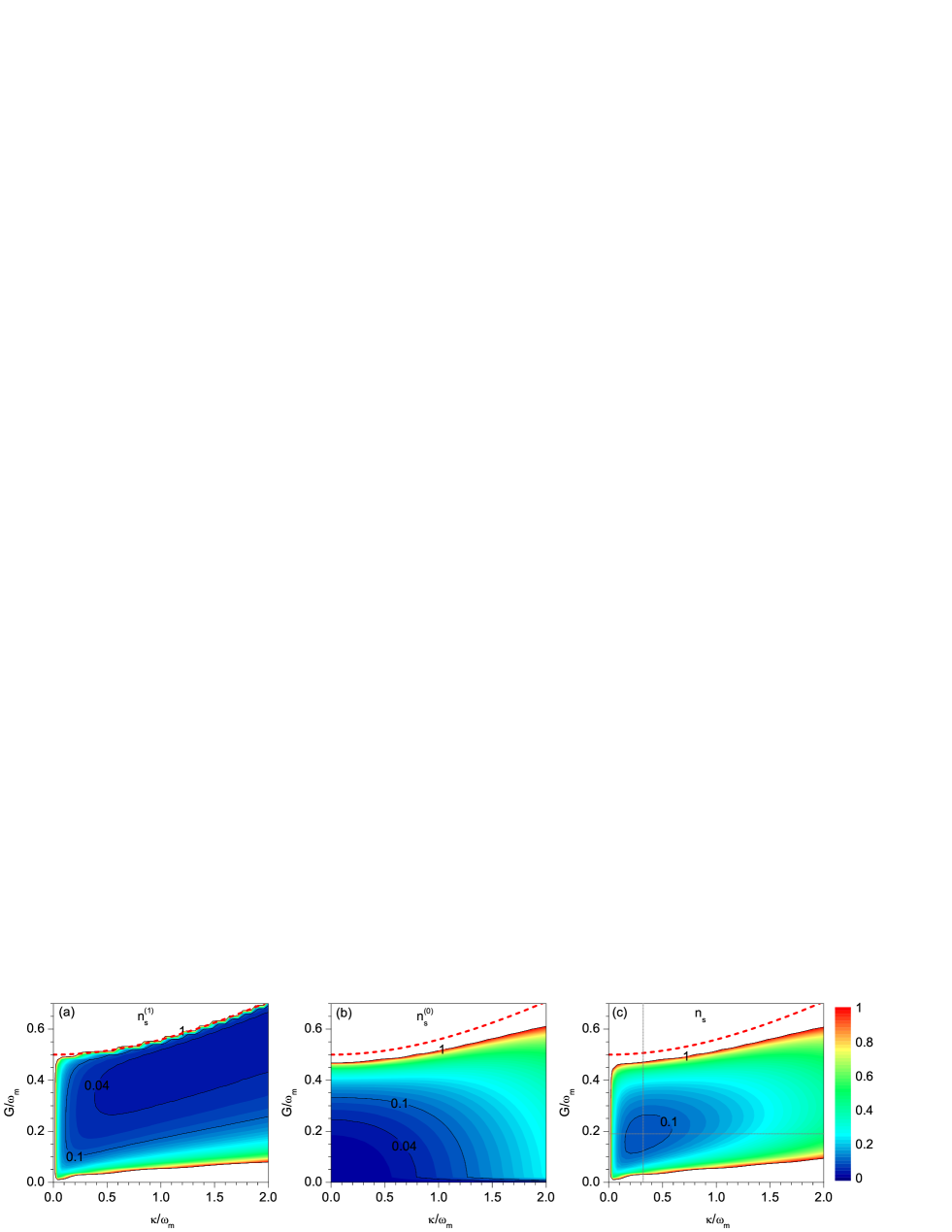
Figure 2: (color online) Steady-state classical cooling limit $n_{\mathrm{s}}^{\mathrm{(1)}}$ (panel a), quantum cooling limit $n_{\mathrm{s}}^{\mathrm{(0)}}$ (panel b) and total cooling limit $n_{\mathrm{s}}$ (panel c) as functions of the cavity decay rate ${\kappa}$ and coupling strength $G$. The red dashed curves correspond to the boundary of the stability condition given by Eq. (1b). In (c), the vertical and horizontal lines denotes the optimal ${\kappa}$ and $G$ given by Eqs. (5a) and (5b). Other parameters: $\Delta^{\prime}=-{\omega_{\mathrm{m}}}$, ${\gamma/\omega_{\mathrm{m}}=10}^{-5}$ and $n_{\mathrm{th}}=10^{3}$.

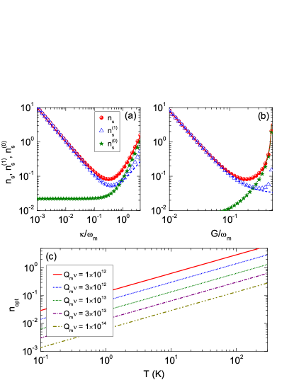
Figure 3: (color online) Cooling limits $n_{\mathrm{s}}$ (red circles and red solid curves), $n_{\mathrm{s}}^{\mathrm{(1)}}$ (blue triangles and blue dashed curves) and $n_{\mathrm{s}}^{\mathrm{(0)}}$ (green stars and green dotted curves) as functions of ${\kappa}$ for $G={G}_{\mathrm{opt}}$ (a) and as functions of $G$ for $\kappa={\kappa}_{\mathrm{opt}}$ (b). The circles, triangles and stars are the numerical results, and the curves are the analytical results given by Eqs. (3a) and (3b). Other parameters: $\Delta^{\prime}=-{\omega_{\mathrm{m}}}$, ${\gamma/\omega_{\mathrm{m}}=10}^{-5}$ and $n_{\mathrm{th}}=10^{3}$. (c) $n_{\mathrm{opt}}$ as a function of the environmental temperature $T$ for $Q_{\mathrm{m}}{\nu=10}^{12}$ (red solid curve), $3\times{10}^{12}$ (blue dashed curve), ${10}^{13}$ (green dotted curve), $3\times{10}^{13}$ (purple dash-dotted curve) and ${10}^{14}$ (orange dash-dot-dotted curve).

In the unresolved sideband regime (${\kappa\gg\omega_{\mathrm{m}}}$) where the mechanical sideband cannot be resolved from cavity mode spectrum, the optimal quantum cooling limit is obtained at the detuning $\Delta^{\prime}=-\kappa/2$ with $n_{\mathrm{s}}^{\mathrm{(0)}}\simeq\kappa/(4{\omega_{\mathrm{m}}})\gg 1$, which prevents ground-state cooling PRL07-1 ; PRL07-2 . Thus, in the following we focus on the resolved sideband regime (${\omega_{\mathrm{m}}\gg\kappa}$). In this case the optimal detunings for both the classical and quantum cooling limits are near $\Delta^{\prime}=-{\omega_{\mathrm{m}}}$, where the rotating-wave interaction characterized by the term $G(a_{1}^{{\dagger}}b_{1}+a_{1}b_{1}^{{\dagger}})$ is on resonant, leading to the maximum energy transfer from the mechanical mode to the anti-Stokes sideband. Meanwhile, the counter-rotating-wave interaction $G(a_{1}^{{\dagger}}b_{1}^{{\dagger}}+a_{1}b_{1})$ is off resonant, which has minor contribution to the heating process. Under the condition ${\omega_{\mathrm{m}}\gg(\kappa,G)\gg\gamma}$ and $\Delta^{\prime}=-{\omega_{\mathrm{m}}}$, we obtain approximate analytical expression of the cooling limits as

$$n_{\mathrm{s}}^{\mathrm{(1)}}\left|{}_{\Delta^{\prime}=-{\omega_{\mathrm{m}}}}\right. \simeq\frac{{4G}^{2}+{\kappa}^{2}}{{4G}^{2}{\kappa}}{\gamma}n_{\mathrm{th}},$$ (3a)

$$n_{\mathrm{s}}^{\mathrm{(0)}}\left|{}_{\Delta^{\prime}=-{\omega_{\mathrm{m}}}}\right. \simeq\frac{{\kappa}^{2}{+}8{G}^{2}}{{16(\omega_{\mathrm{m}}^{2}-4G}^{2})},$$ (3b)

These limits are valid in the weak, intermediate and strong coupling regimes. In particular, in the weak coupling regime ($${\kappa\gg G} n_{\mathrm{s}}^{\mathrm{(1)}}\simeq n_{\mathrm{th}}{\gamma\kappa}/({4G}^{2}) n_{\mathrm{s}}^{\mathrm{(0)}}\simeq{\kappa}^{2}/{(16\omega_{\mathrm{m}}^{2}}) {G\gg\kappa} n_{\mathrm{s}}^{\mathrm{(1)}}\simeq n_{\mathrm{th}}{\gamma}/{\kappa} n_{\mathrm{s}}^{\mathrm{(0)}}\simeq{G}^{2}/[2{(\omega_{\mathrm{m}}^{2}-4G}^{2})]$$), the cooling limits reduce to and , which agree with the perturbation approaches PRL07-1 ; PRL07-2 . For strong coupling regime (), the cooling limits are simplified as and .

In Fig. 2 we plot the exact numerical results of the cooling limits $n_{\mathrm{s}}^{\mathrm{(1)}}$, $n_{\mathrm{s}}^{\mathrm{(0)}}$ and $n_{\mathrm{s}}$ as functions of ${\kappa}$ and $G$ for $\Delta^{\prime}=-{\omega_{\mathrm{m}}}$, ${\gamma/\omega_{\mathrm{m}}=10}^{-5}$ and $n_{\mathrm{th}}=10^{3}$. For the classical cooling limit $n_{\mathrm{s}}^{\mathrm{(1)}}$, within the stable region, a larger ${G}$ and a larger $\kappa$ lead to a lower cooling limit, as shown in Fig. 2(a). Note that the classical cooling limit can be expressed as $n_{\mathrm{s}}^{\mathrm{(1)}}=n_{\mathrm{th}}{\gamma/\Gamma}$, where ${\Gamma}$ is the optical damping rate (net cooling rate) given by

$$\frac{{1}}{{\Gamma}}=\frac{{1}}{{\Gamma}_{\mathrm{wk}}}+\frac{{1}}{{\Gamma}_{\mathrm{str}}},$$ (4a)

$${\Gamma}_{\mathrm{wk}}=\frac{{4G}^{2}}{{\kappa}},\text{ \ }{\Gamma}_{\mathrm{str}}={\kappa.}$$ (4b)

Here $${\Gamma}_{\mathrm{opt}}^{\mathrm{wk}} {\Gamma}_{\mathrm{opt}}^{\mathrm{str}} {G}^{2}/{\kappa} {\kappa}$$ and represent the optical damping rate in the weak and strong coupling regimes, respectively. Therefore, for the weak coupling case, to obtain a high cooling rate, one expect a large ; while in the strong coupling regime, a large leads to a high cooling rate.

On the other hand, large $G$ and large $\kappa$ result in higher quantum cooling limit $n_{\mathrm{s}}^{\mathrm{(0)}}$ due to stronger quantum backaction, as plotted in Fig. 2(b). These trade-offs result in optimal $\kappa$ and $G$ for the total cooling limit $n_{\mathrm{s}}$, which can be approximately derived as

$${\kappa}_{\mathrm{opt}} \simeq 1.5{\omega_{\mathrm{m}}}(\frac{n_{\mathrm{th}}}{Q_{\mathrm{m}}})^{\frac{1}{3}}{,}$$ (5a)

$${G}_{\mathrm{opt}} \simeq 0.9{\omega_{\mathrm{m}}}(\frac{n_{\mathrm{th}}}{Q_{\mathrm{m}}})^{\frac{1}{3}},$$ (5b)

where $$Q_{\mathrm{m}}={\omega_{\mathrm{m}}/\gamma} {G}_{\mathrm{opt}}\sim 0.6{\kappa}_{\mathrm{opt}} \kappa={\kappa}_{\mathrm{opt}} G={G}_{\mathrm{opt}}$$ denotes the mechanical quality factor. It shows that , indicating the intermediate coupling. The gray dotted vertical and horizontal lines in Fig. 2(c) denote and , which agree well with the numerical results.

In Fig. 3 we further plot $n_{\mathrm{s}}^{\mathrm{(1)}}$, $n_{\mathrm{s}}^{\mathrm{(0)}}$ and $n_{\mathrm{s}}$ for optimized $G$ and ${\kappa}$, along the horizontal and vertical lines in Fig. 2(c), respectively. It shows that classical cooling limit dominates for small $\kappa$ and $G$, while quantum cooling limit becomes important as $\kappa$ and $G$ increase, which are precisely described by Eqs. (3a) and (3b).

With the optimal parameters given in Eqs. (5a) and (5b), the optimal cooling limit reads

$$n_{\mathrm{opt}}\simeq 1.8(\frac{n_{\mathrm{th}}}{Q_{\mathrm{m}}})^{\frac{2}{3}}.$$ (6)

In Fig. 3(c) we plot $n_{\mathrm{opt}}$ as a function of the environmental temperature $T$ for various $Q$-frequency products. It shows that a high $Q$-frequency product allows for achieving a low phonon number at a high temperature region. For ground-state cooling (or ground-state occupancy probability $P>50\%$), it requires

$$Q_{\mathrm{m}}>2.4n_{\mathrm{th}}.$$ (7)

For typical mechanical resonators, $\hbar{\omega_{\mathrm{m}}\ll k}_{\mathrm{B}}T$, and the thermal phonon number is approximated as $n_{\mathrm{th}}\simeq{k}_{\mathrm{B}}T/(\hbar{\omega_{\mathrm{m}}})$. Therefore, the condition (7) is equivalent to $Q_{\mathrm{m}}{\omega_{\mathrm{m}}>}2.4{k}_{\mathrm{B}}T/\hbar$. Starting from room temperature ($T=300$ $\mathrm{K}$), the requirement for ground-state cooling is expressed by the $Q$-frequency product

$$Q_{\mathrm{m}}{\nu>1.5}\times 10^{13},$$ (8)

where ${\nu=\omega_{\mathrm{m}}/}2\pi$ is the mechanical resonance frequency.

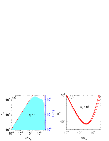
Figure 4: (color online) (a) Contour plot of the ground-state region ($n_{\mathrm{s}}<1$) as functions of ${\kappa}$ and $n_{\mathrm{th}}$. The shaded region corresponds to $n_{\mathrm{s}}<1$. The red dashed lines denote ${\kappa=\gamma}n_{\mathrm{th}}$ (left) and ${\kappa=4\omega_{\mathrm{m}}}$ (right), respectively. (b) Cooling limit $n_{\mathrm{s}}$ as a function of ${\kappa}$ for $n_{\mathrm{th}}=10^{3}$. The red circles are the numerical results and the red solid curve corresponds to the analytical results given by Eqs. (3a) and (3b). Other parameters: $\Delta^{\prime}=-{\omega_{\mathrm{m}}}$, ${\gamma/\omega_{\mathrm{m}}=10}^{-5}$ and ${G=G}_{\mathrm{opt}}({\kappa})$ [given by Eq. (9)].

In real experiments, there are restrictions on the cavity decay rate $\kappa$ and the coupling strength $G$. For example, many optical cavities have lower bounds for $\kappa$ due to the limitation of fabrication and material absorption. The coupling strength $G$ is related to the intracavity optical field, while strong light field usually leads to material absorption and heating. Therefore, it is important to take these constraints into consideration. In the following we provide the parameter range for $\kappa$ and $G$ where ground-state cooling can be reached.

First we consider the requirement for the cavity decay rate $\kappa$. The optimal coupling strength $G$ for a given ${\kappa}$ is obtained as

$${G}_{\mathrm{opt}}({\kappa})\simeq(\frac{{\omega_{\mathrm{m}}^{2}\kappa\gamma}n_{\mathrm{th}}}{2})^{\frac{1}{4}}.$$ (9)

Under this condition, ground-state cooling requires

$${\gamma}n_{\mathrm{th}}<{\kappa<4\omega_{\mathrm{m}}}.$$ (10)

The left inequality reveals that the cavity decay rate should exceed the thermal decoherence rate ${\Gamma}_{\mathrm{th}}={\gamma}n_{\mathrm{th}}$ to suppress the environmental heating. The requirement can be re-expressed as $Q_{\mathrm{m}}{\kappa>k}_{\mathrm{B}}T/\hbar$. At room temperature, it yields

$$Q_{\mathrm{m}}{\kappa>6.2}\times 10^{12}\text{.}$$ (11)

The right inequality in Eq. (10) shows that the resolved sideband condition should be satisfied to reduce the quantum backaction heating. In Fig. 4(a) the exact numerical results for the ground-state region is plotted, with the region boundary well described by Eq. (10). As an example, we plot the cooling limit $n_{\mathrm{s}}$ as a function of ${\kappa}$ for ${\gamma/\omega_{\mathrm{m}}=10}^{-5}$ and $n_{\mathrm{th}}=10^{3}$. In this case $n_{\mathrm{s}}<1$ requires ${0.01}<{\kappa/\omega_{\mathrm{m}}<4}$.

To obtain the requirement for the coupling strength $G$, we determine the optimal cavity decay rate $\kappa$ for a given $G$ as

$${\kappa}_{\mathrm{opt}}({G})\simeq 2G.$$ (12)

Then the requirement for ground-state cooling is given by

$${\gamma}n_{\mathrm{th}}<{G<0.5\omega_{\mathrm{m}}}.$$ (13)

Clearly, the coupling strength should also exceed the thermal decoherence rate to suppress the environmental heating, and room-temperature ground-state cooling requires

$$Q_{\mathrm{m}}{G>6.2}\times 10^{12}.$$ (14)

The upper restriction ${G<0.5\omega_{\mathrm{m}}}$ is limited by the stability condition given by Eq. (1b). In Fig. 5(a) the exact numerical results for the ground-state region is plotted, with the region boundary well described by Eq. (13). A example for $n_{\mathrm{th}}=10^{3}$ is shown in Fig. 5(b).

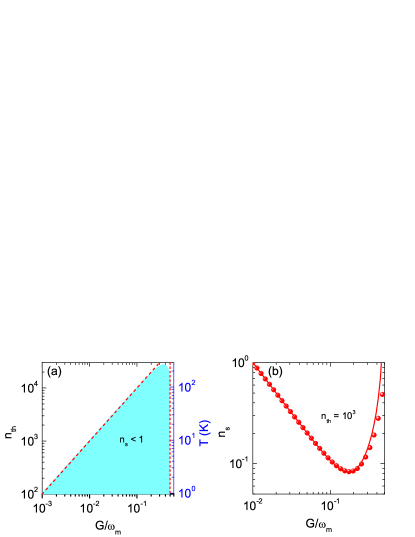
Figure 5: (color online) Same as Fig. 4 except that the horizontal axes are ${G}$ and the value of the cavity decay rate is ${\kappa=\kappa}_{\mathrm{opt}}({G})$ [given by Eq. (12)]. In (a), the red dashed lines denote ${G=\gamma}n_{\mathrm{th}}$ (left) and ${G=0.5\omega_{\mathrm{m}}}$ (right), respectively.

In summary, we have examined the backaction cooling of mesoscopic mechanical resonators in the intermediate coupling regime. We develop a general framework to describe the steady-state backaction cooling limits in the full parameter range. We have analytically derived the optimal cooling limits and the optimal parameters including the cavity decay rate and the optomechanical coupling strength. In the resolved sideband regime, under the optimal detuning $\Delta^{\prime}=-{\omega_{\mathrm{m}}}$, the optimal cavity decay rate and the optimal coupling strength are derived as ${\kappa}_{\mathrm{opt}}\simeq 1.5{\omega_{\mathrm{m}}}(n_{\mathrm{th}}/Q_{\mathrm{m}})^{1/3}$ and ${G}_{\mathrm{opt}}\simeq 0.9{\omega_{\mathrm{m}}}(n_{\mathrm{th}}/Q_{\mathrm{m}})^{1/3}$, with the lowest cooling limit being $n_{\mathrm{opt}}\simeq 1.8(n_{\mathrm{th}}/Q_{\mathrm{m}})^{2/3}$. At the optimal point, the requirement for ground-state cooling is $Q_{\mathrm{m}}>2.4n_{\mathrm{th}}$. Starting from room temperature, ground-state cooling is achievable for mechanical $Q$-frequency product $Q_{\mathrm{m}}{\nu>1.5}\times 10^{13}$. For practical optomechanical systems, the allowed parameter regions for ground-state cooling are $\gamma n_{\mathrm{th}}<{\kappa<4\omega_{\mathrm{m}}}$ and $\gamma n_{\mathrm{th}}<{G<0.5\omega_{\mathrm{m}}}$. This provides a guideline for achieving the lowest cooling limit towards room-temperature ground-state cooling of mechanical resonators.

- (1) T. J. Kippenberg and K. J. Vahala, Science 321, 1172 (2008).
- (2) F. Marquardt and S. M. Girvin, Physics 2, 40 (2009).
- (3) P. Meystre, Ann. Phys. (Berlin) 525, 215 (2013).
- (4) M. Aspelmeyer, T. J. Kippenberg, F. Marquardt, arXiv:1303.0733 (2013).
- (5) Y.-C. Liu, Y.-W. Hu, C. W. Wong and Y.-F. Xiao, Chin. Phys. B 22, 114213 (2013).
- (6) J. D. Teufel, T. Donner, D. Li, J. W. Harlow, M. S. Allman, K. Cicak, A. J. Sirois, J. D. Whittaker, K. W. Lehnert, and R. W. Simmonds, Nature (London) 475, 359 (2011).
- (7) J. Chan, T. P. Mayer Alegre, A. H. Safavi-Naeini, J. T. Hill, A. Krause, S. Gröblacher, M. Aspelmeyer, and O. Painter, Nature (London) 478, 89 (2011).
- (8) O. Romero-Isart, A. C. Pflanzer, F. Blaser, R. Kaltenbaek, N. Kiesel, M. Aspelmeyer, and J. I. Cirac, Phys. Rev. Lett. 107, 020405 (2011).
- (9) B. Pepper, R. Ghobadi, E. Jeffrey, C. Simon, and D. Bouwmeester, Phys. Rev. Lett. 109, 023601 (2012).
- (10) Z.-q. Yin, T. Li, X. Zhang, and L. M. Duan, Phys. Rev. A 88, 033614 (2013).
- (11) S. Mancini, D. Vitali, and P. Tombesi, Phys. Rev. Lett. 90, 137901 (2003).
- (12) K. Stannigel, P. Rabl, A. S. Sørensen, P. Zoller, and M. D. Lukin, Phys. Rev. Lett. 105, 220501 (2010).
- (13) K. Stannigel, P. Komar, S. J. M. Habraken, S. D. Bennett, M. D. Lukin, P. Zoller, and P. Rabl, Phys. Rev. Lett. 109, 013603 (2012).
- (14) A. D. O’Connell, M. Hofheinz, M. Ansmann, R. C. Bial-czak, M. Lenander, E. Lucero, M. Neeley, D. Sank, H.Wang, M. Weides, J. Wenner, John M. Martinis, and A.N. Cleland, Nature (London) 464, 697 (2010).
- (15) S. Mancini, D. Vitali, and P. Tombesi, Phys. Rev. Lett. 80, 688 (1998).
- (16) P.-F. Cohadon, A. Heidmann, and M. Pinard, Phys. Rev. Lett. 83, 3174 (1999).
- (17) D. Kleckner and D. Bouwmeester, Nature 444, 75 (2006).
- (18) T. Corbitt, C. Wipf, T. Bodiya, D. Ottaway, D. Sigg, N. Smith, S. Whitcomb, and N. Mavalvala, Phys. Rev. Lett. 99, 160801 (2007).
- (19) M. Poggio, C. L. Degen, H. J. Mamin, and D. Rugar, Phys. Rev. Lett. 99, 17201 (2007).
- (20) S. Gigan, H. R. Böhm, M. Paternostro, F. Blaser, G. Langer, J. B. Hertzberg, K. C. Schwab, D. Bäuerle, M. Aspelmeyer, and A. Zeilinger, Nature (London) 444, 67 (2006).
- (21) O. Arcizet, P.-F. Cohadon, T. Briant, M. Pinard, and A. Heidmann, Nature (London) 444, 71 (2006).
- (22) A. Schliesser, P. Del’Haye, N. Nooshi, K. J. Vahala, and T. J. Kippenberg, Phys. Rev. Lett. 97, 243905 (2006).
- (23) A. Schliesser, R. Rivière, G. Anetsberger, O. Arcizet, and T. J. Kippenberg, Nature Phys. 4, 415 (2008).
- (24) S. Gröblacher, J. B. Hertzberg, M. R. Vanner, G. D. Cole, S. Gigan, K. C. Schwab, and M. Aspelmeyer, Nature Phys. 5, 485 (2009).
- (25) Y.-S. Park and H. Wang, Nature Phys. 5, 489 (2009).
- (26) A. Schliesser, O. Arcizet, R. Rivère, G. Anetsberger, and T. J. Kippenberg, Nature Phys. 5, 509 (2009).
- (27) T. Rocheleau, T. Ndukum, C. Macklin, J. B. Hertzberg, A. A. Clerk, and K. C. Schwab, Nature (London) 463, 72 (2010).
- (28) R. Riviere, S. Deleglise, S. Weis, E. Gavartin, O. Arcizet, A. Schliesser, and T. Kippenberg, Phys. Rev. A 83, 063835 (2011).
- (29) F. Elste, S. M. Girvin, and A. A. Clerk, Phys. Rev. Lett. 102, 207209 (2009).
- (30) M. Li, W. H. P. Pernice, and H. X. Tang, Phys. Rev. Lett. 103, 223901 (2009).
- (31) A. Xuereb, R. Schnabel, and K. Hammerer, Phys. Rev. Lett. 107, 213604 (2011).
- (32) T. Weiss and A. Nunnenkamp, Phys. Rev. A 88, 023850 (2013).
- (33) M.-Y. Yan, H.-K. Li, Y.-C. Liu, W.-L. Jin, and Y.-F. Xiao, Phys. Rev. A 88, 023802 (2013).
- (34) A. Nunnenkamp, K. Børkje, J. G. E. Harris, and S. M. Girvin, Phys. Rev. A 82, 021806(R) (2010).
- (35) A. Nunnenkamp, K. Børkje, and S. M. Girvin, Phys. Rev. A 85, 051803(R) (2012).
- (36) C. Genes, H. Ritsch, and D. Vitali, Phys. Rev. A 80, 061803(R) (2009).
- (37) B. Vogell, K. Stannigel, P. Zoller, K. Hammerer, M. T. Rakher, M. Korppi, A. Jöckel, and P. Treutlein, Phys. Rev. A 87, 023816 (2013).
- (38) M. R. Vanner, I. Pikovski, G. D. Cole, M. S. Kim, Č. Brukner, K. Hammerer, G. J. Milburn, and M. Aspelmeyer, Proc. Natl. Acad. Sci. USA 108, 16182 (2011).
- (39) Y. Li, L.-A. Wu, and Z. D. Wang, Phys. Rev. A 83, 043804 (2011).
- (40) J.-Q. Liao and C. K. Law, Phys. Rev. A 84, 053838 (2011).
- (41) X. Wang, S. Vinjanampathy, F. W. Strauch, and K. Jacobs, Phys. Rev. Lett. 107, 177204 (2011).
- (42) S. Machnes, J. Cerrillo, M. Aspelmeyer, W. Wieczorek, M. B. Plenio, and A. Retzker, Phys. Rev. Lett. 108, 153601 (2012).
- (43) Y.-C. Liu, Y.-F. Xiao, X. Luan, and C. W. Wong, Phys. Rev. Lett. 110, 153606 (2013).
- (44) I. Wilson-Rae, N. Nooshi, W. Zwerger, and T. J. Kippenberg, Phys. Rev. Lett. 99, 093901 (2007).
- (45) F. Marquardt, J. P. Chen, A. A. Clerk, and S. M. Girvin, Phys. Rev. Lett. 99, 093902 (2007).
- (46) C. Genes, D. Vitali, P. Tombesi, S. Gigan, and M. Aspelmeyer, Phys. Rev. A 77, 033804 (2008).
- (47) J. M. Dobrindt, I. Wilson-Rae, and T. J. Kippenberg, Phys. Rev. Lett. 101, 263602 (2008).
- (48) I. Wilson-Rae, N. Nooshi, J. Dobrindt, T. J. Kippenberg and W. Zwerger, New J. Phys. 10, 095007 (2008).
- (49) S. Gröblacher, K. Hammerer, M. R. Vanner, and M. Aspelmeyer, Nature (London) 460, 724 (2009).
- (50) J. D. Teufel, D. Li, M. S. Allman, K. Cicak, A. J. Sirois, J. D. Whittaker, and R. W. Simmonds, Nature (London) 471, 204 (2011).
- (51) E. Verhagen, S. Deléglise, S. Weis, A. Schliesser, and T. J. Kippenberg, Nature (London) 482, 63 (2012).
- (52) T. A. Palomaki, J. W. Harlow, J. D. Teufel, R. W. Simmonds, and K. W. Lehnert, Nature (London) 495, 210 (2013).
- (53) S. Chakram, Y. S. Patil, L. Chang, and M. Vengalattore, Phys. Rev. Lett. 112, 127201 (2014).
- (54) C. K. Law, Phys. Rev. A 51, 2537 (1995).
- (55) Y.-C. Liu, Y.-F. Shen, Q. Gong and Y.-F. Xiao, Phys. Rev. A 89, 053821 (2014).
- (56) E. X. DeJesus and C. Kaufman, Phys. Rev. A 35, 5288 (1987).