Trumpeting M Dwarfs with CONCH-SHELL: a Catalog of Nearby Cool Host-Stars for Habitable ExopLanets and Life

Abstract

We present an all-sky catalog of 2970 nearby ($d\lesssim 50$ pc), bright ($J<9$) M- or late K-type dwarf stars, 86% of which have been confirmed by spectroscopy. This catalog will be useful for searches for Earth-size and possibly Earth-like planets by future space-based transit missions and ground-based infrared Doppler radial velocity surveys. Stars were selected from the SUPERBLINK proper motion catalog according to absolute magnitudes, spectra, or a combination of reduced proper motions and photometric colors. From our spectra we determined gravity-sensitive indices, and identified and removed 0.2% of these as interloping hotter or evolved stars. Thirteen percent of the stars exhibit H${\alpha}$ emission, an indication of stellar magnetic activity and possible youth. The mean metallicity is [Fe/H] = -0.07 with a standard deviation of 0.22 dex, similar to nearby solar-type stars. We determined stellar effective temperatures by least-squares fitting of spectra to model predictions calibrated by fits to stars with established bolometric temperatures, and estimated radii, luminosities, and masses using empirical relations. Six percent of stars with images from integral field spectra are resolved doubles. We inferred the planet population around M dwarfs using Kepler data and applied this to our catalog to predict detections by future exoplanet surveys.

1 Introduction

The NASA Kepler mission monitored approximately 200,000 stars for transiting planets, and thousand of candidate planets have been identified in the light curves (Rowe et al., 2014). A few hundred of these have been vetted and the overall rate of false positives is generally, but not uniformly, low (Santerne et al., 2012; Colón, Ford & Morehead, 2012; Fressin et al., 2013). Statistical analysis of the candidates shows that at least half of stars host planets with orbital periods less than $\sim$200 d and that Earth- to Neptune-size planets are far more numerous than Jupiter-size planets (e.g. Howard et al., 2012; Fressin et al., 2013). Some Kepler-detected planets orbiting very cool (late K- and M-type) dwarfs are near or inside the theoretical “habitable zones” of these stars where an Earth-like planet could have liquid water on its surface (Dressing & Charbonneau, 2013; Kopparapu, 2013; Gaidos, 2013; Quintana et al., 2014). But Kepler planet-hosting stars are typically distant (hundreds or thousands of pc) and faint ($V\sim 15$), making measurement of mass by Doppler radial velocity (RV, e.g. Marcy et al., 2014) or follow-up such as transit spectroscopy or observations of secondary eclipse difficult or impossible.

The Kepler field covers only 0.25% of the sky and, ironically, we know much less about Earth- to Neptune-size planets around nearby stars, including those around very cool dwarfs. The RV method can be readily applied to nearby stars which are widely spaced on the sky, but because of the scaling between planet mass and radius, it is comparatively less sensitive to smaller planets than the transit method. The most sensitive RV surveys have found a few super-Earths on close orbits around M dwarfs (Bonfils et al., 2013) but such surveys have been hampered by the faintness of such stars at visible wavelengths. Ground-based, wide-field transit surveys are affected by correlated (“red”) noise from the atmosphere and can only detect short-period giant planets around F and G dwarfs. Transit surveys of nearby very cool dwarfs using individual pointings have met with limited success (Berta, Irwin & Charbonneau, 2013; Gaidos et al., 2014).

Our knowledge of nearby small planets should dramatically improve with two developments: the deployment of infrared Doppler spectrographs that can exploit a spectral range where M dwarfs are brighter (Tamura et al., 2012; Thibault et al., 2012; Mahadevan et al., 2012; Quirrenbach et al., 2012), and the launch of the NASA Transiting Exoplanet Survey Satellite mission (TESS, Ricker et al., 2010). In principle these surveys will detect nearby Earth- or super-Earth-size planets on close-in orbits around the brightest M dwarfs and/or measure their mass. But until recently, no all-sky catalog of well-characterized M dwarfs suitable as a source of targets was available. Lépine & Gaidos (2011, hereafter LG11) published a catalog of 8889 bright ($J<10$), nearby late K- and early M-type dwarfs selected from the SUPERBLINK proper motion catalog (Lépine & Shara, 2005) using proper motions and $V$-$J$ and $JHK_{S}$ colors. This was followed by a spectroscopic survey of all the northern LG11 stars with $J<9$ (Lépine et al., 2013). Frith et al. (2013, ,hereafter F13) also produced a catalog of bright ($K_{S}<9$) M dwarf candidates based on the PPMXL catalog (Roeser, Demleitner & Schilbach, 2010).

Although these catalogs represent advances in cataloging and describing the nearest M dwarf stars, there is still room for improvement. The spectroscopic catalog of Lépine et al. (2013) only included stars at declinations $\delta>0$. The conservative infrared color cuts imposed by LG11 to weed out giant stars also eliminated some metal-rich dwarf stars which have red $J$-$H$ and $H$-$K_{S}$ colors (Leggett, 1992; Newton et al., 2014). These metal-rich dwarfs are more likely to host giant planets (Johnson & Apps, 2009; Rojas-Ayala et al., 2010; Mann et al., 2013b), e.g. HIP 79431 (Apps et al., 2010). Finally, visible-wavelength ($BVg^{\prime}r^{\prime}i^{\prime}$) photometry is now available for most bright stars from the AAVSO Photometric All Sky Survey (APASS, Henden et al., 2012). This CCD photometry is much more precise ($\geq 0.02$ magnitudes) than the photographic plate-based United States Naval Observatory (Monet et al., 2003, USNO-B,) magnitudes used for most LG11 stars. These data allow for more accurate elimination of hotter or evolved stars based on photometric colors and magnitudes.

For these reasons we have constructed a revised catalog, which we call CONCH-SHELL (Catalog Of Nearby Cool Host-Stars for Habitable ExopLanets and Life). CONCH-SHELL is selected from the SUPERBLINK catalog using modified criteria and new photometry and spectroscopy (Section 2). Including previous data, we obtained moderate-resolution ($\lambda/\Delta\lambda\sim 10^{3}$) spectra of 86% of the catalog (Section 3). We used spectra to measure gravity-sensitive indicators, confirm the dwarf luminosity class of these stars, and estimate their spectral type, effective temperature, and metallicity (Section 4). For most stars we measured any H$\alpha$ emission, an indicator of stellar activity, and limited imaging of some stars allowed us to identify binaries. We combined effective temperatures with empirical relations derived from observations of calibrator stars to estimate stellar radius, luminosity, and mass. We compared our catalog with F13 (Section 5). We estimated the yield of transiting planets that might be detected by TESS and future infrared Doppler observations of these stars (Section 6.1). We summarize the properties of our catalog and the potential for future follow-up observations in Section 7.

2 Catalog Construction

LG11 selected candidate M dwarfs as stars that were (i) bright ($J<10$) (ii) red ($V-J>2.7$), (iii) have absolute magnitudes or reduced proper motions, proxies for absolute magnitudes, consistent with the main sequence and (iv) infrared Two Micron All-Sky Survey (2MASS, Skrutskie et al., 2006) $JHK_{S}$ colors that are consistent with M dwarfs. Lépine et al. (2013) obtained spectra of the brightest ($J<9$) LG11 stars in the northern celestial hemisphere and showed that they were virtually all M dwarfs. In this work, we constructed a revised catalog of $J<9$ M dwarfs using modified criteria and new photometry from APASS. Our criteria are based on a subset of stars confirmed by either parallaxes or spectra from Lépine et al. (2013).

We examined 21901 proper-motion stars in the SUPERBLINK catalog (Lépine & Shara, 2005) with $J<9$, $J$-$K_{s}>0.65$ and proper motion $\mu>$ 40 mas yr^-1 (north of -20^∘) or $\mu>80$ mas yr^-1 (south). The north-south difference in proper motion limits reflects the higher reliability of the SUPERBLINK catalog in the north. Positions and $JHK_{s}$ magnitudes and their errors were obtained by matching stars to 2MASS sources after correcting for proper motion over the difference of the 2MASS observation epoch and 2000. Our matching criterion was based on the distribution of separations was 1 arc-sec and we flagged stars where the angular separation is larger. Six stars with magnitudes flagged in the 2MASS catalog as being of poor quality or upper limits due to detector nonlinearity are not used in computing infrared colors (see below), but we do use the $J$ magnitudes in such cases because an upper limit only means that the star is even brighter and redder than stated. Photographic visual magnitudes $V_{E}$ were generated for all stars from USNO-B $b$ and $r$ magnitudes and 2MASS $J$ magnitudes according to the prescription in Lépine & Shara (2005).

We matched selected SUPERBLINK stars to the revised version of the Hipparcos catalog (van Leeuwen, 2007), the Tycho-2 catalog (Høg et al., 2000), the APASS catalog (Date Release 7), and the All-Sky Compiled Catalogue Version 2.5 (ASCC-2.5, Kharchenko & Roeser, 2009). The last catalog includes both Hipparcos and Tycho-2 so there is some redundancy. The Hipparcos catalog was matched to the SUPERBLINK stars assuming an observation epoch of 1992.25, calculated by minimizing the median angular separation of matches, and differing slightly from the nominal catalog epoch of 1991.25. Based on the distribution of matches, we applied a matching criterion of $<1.3$ arcsec in angular separation and less than one magnitude difference in Hipparcos $V$ vs. $V_{E}$. Likewise, we used matching criteria of 1.3 arcsec and 1.2 magnitudes for the Tycho-2 catalog. We found that the catalog epoch that minimized the median angular separation was 1992.3, close to the Hipparcos epoch but much earlier than the 2000 epoch given in the catalog’s documentation. For APASS matches, we required that $0.8<i-J<2.8$ ($i$ from APASS and $J$ from 2MASS) and an angular separation $<2.5$ arcsec. If there was more than one match to any star in the APASS catalog (25 cases) only the closest match was considered, and we flagged these cases.

Tycho-2 magnitudes were adjusted to the Johnson system using the relationship in the Appendix of Mamajek, Meyer & Liebert (2002). About 5% of stars have APASS $V<10$ and we adjusted APASS $V$ magnitudes for nonlinearity by comparing with Hipparcos photometry, calculating a running median with a 0.25-magnitude bin, and fitting a line with iterative 3$\sigma$ rejection of points. The APASS-Hipparcos offset at $V=11.2$ is only -0.093 magnitudes and the slope is 0.038 mag mag^-1. We then calculated a color correction to convert $V_{E}$ magnitudes to corrected APASS magnitudes by a linear fit to the median difference vs. $V_{E}-J$ color in 0.2 magnitude bins. The APASS-$V_{E}$ offset at $V_{E}-J=2.7$ is 0.081 magnitudes, and the slope is -0.174 mag mag^-1. The latter is apparently due to imperfect calibration of $V_{E}$ against $V$ in Lépine & Shara (2005). Visual magnitudes, as available, were assigned to stars in the following order of decreasing priority: Hipparcos, APASS, Tycho-2, and USNO-B.

We used parallaxes from the Hipparcos catalog as well as from Harrington et al. (1993); van Altena, Lee & Hoffleit (1995); McCook & Sion (1999); Myers et al. (2001); Costa et al. (2005); Jao et al. (2005); Costa et al. (2006); Henry et al. (2006); Smart et al. (2007); Gatewood (2008); Gatewood & Coban (2009); Khrutskaya, Izmailov & Khovrichev (2010); Riedel et al. (2010); Jao et al. (2011) and Dittmann et al. (2014). Some stars are proper motion companions to Hipparcos stars and so have precise parallaxes but no Hipparcos numbers.

Absolute magnitudes $M_{V}$ were calculated for 9567 stars in the input catalog with parallaxes. These are plotted vs. $V$-$J$ color in Fig. 1. To describe the main sequence locus for $M_{V}$ vs. $V$-$J$ we iteratively fit a quadratic formula to median values in a running 0.2 magnitude-wide bin with color. The intrinsic scatter (standard deviation) of the locus after accounting for errors in $M_{V}$ was re-computed for each iteration and only stars within three standard deviations of the locus (where errors and intrinsic scatter were added in quadrature) were retained for the next iteration. The final locus had an intrinsic width of 0.46 magnitudes, presumably due to the metallicity dependence of luminosity and unresolved binaries. We selected 1321 stars with $V$-$J>2.7$ and having $M_{V}$ within $3\sigma$ of the final locus and more than $3\sigma$ fainter than $M_{V}=4.2$ (a threshold for identifying evolved stars) as M dwarfs. To these were added 622 stars with $V$-$J>2.7$ that were spectoscopically confirmed as M dwarfs in Lépine et al. (2013). These 1943 stars are plotted as the red points in Fig. 1.

We identified additional M dwarfs lacking measured parallaxes based on their reduced proper motions:

$$H_{V}=V+5\log\mu+5.$$ (1)

Stars with large proper motions, i.e. $H_{V}$ fainter than the main sequence $M_{V}$ for their $V$-$J$ color, plus an offset, were selected as M dwarfs (Fig. 2). We chose the offset to be 0.5 magnitudes based on an inspection of the distribution of $H_{V}-M_{V}$ values. This criterion corresponds to a minimum transverse velocity with respect to the Sun of 6 km sec^-1. The solar peculiar velocity with respect to the Local Standard of Rest is itself about 18 km sec^-1 (Schönrich, Binney & Dehnen, 2010) so this criterion should not eliminate many M dwarfs (see Section 7 for a discussion of catalog completeness).

To eliminate interloping giant stars, candidate M dwarfs were also subjected to photometric color criteria developed using the colors of bona fide M dwarfs identified by absolute magnitudes or spectroscopy. We found that M dwarfs identified by absolute magnitude or spectrum have a narrow range of $J$-$K_{S}$ colors compared to giant stars, with a mean $J$-$K_{S}$=0.83, after eliminating outliers, and an intrinsic dispersion of 0.028 magnitudes, after accounting for measurement error (Fig. 3). Stars with $J$-$K_{S}$ colors falling more than three standard deviations from the locus (with photometry errors and intrinsic dispersion added in quadrature) were excluded.

We also applied criteria using $g-r$ and $r-J$ colors for those stars where APASS photometry is available (Fig. 4). We fit a fifth-order polynomial to the median of $g-r$ values with low error ($<0.03$ magnitudes) in $r-J$ bins. The intrinsic dispersion about this fit is 0.054 magnitudes. Stars with $r-J<2.7$ or $g-r$ magnitudes more than three standard deviations (photometric error and intrinsic dispersion added in quadrature) were excluded. The trajectory of colors of M0-M6 dwarfs from the Sloan Digital Sky Survey (SDSS, Bochanski, Hawley & West, 2011, grey line in Fig. 4) clearly shows that APASS colors differ systematically from SDSS colors and that the discrepancy increases with later spectral type.

We identified additional stars that had $M_{V}$ or $H_{V}$ values that are brighter than the limits described above, but are still consistent with the properties of M dwarfs if significant extinction or large errors in $V$ or $J$ magnitudes are allowed, or they are especially young and luminous, and/or are unresolved binaries. USNO-B-based errors in $V$ may be as large as one magnitude; error in $V$ is represented by slope-one lines in plots of $M_{V}$ or $H_{V}$ vs. $V$-$J$ (Figs 1 and 2). There are six stars in CONCH-SHELL with 2MASS $J$ magnitudes flagged as having low quality or being upper limits: a few stars are bright enough that 2MASS observations may have been in the detector’s nonlinear regime or even saturated. That leads to more uncertain $J$ magnitudes which will displace these stars along slope-one lines in Figs. 1 and 2. In principle, interestellar or circumstellar extinction could also displace stars off the main sequence locus. Based on coefficients appropriate for the interstellar medium (ISM) (Yuan, Liu & Xiang, 2013), the direction of extinction/reddening (arrows) has a slope of 1.25 in Figs. 1 and 2. Such stars are also captured by this criterion.

On the other hand, distant and extincted giant stars or hotter dwarfs would also be displaced to fainter magnitudes and redder colors along the direction of the arrows in Figs. 1-4 and could contaminate the M dwarf catalog. The $J<9$ magnitude limit of the catalog plus the relationship between distance and interstellar extinction limits this effect to stars with the bluest $V$-$J$ colors in our sample. We derived a relationship for the maximum plausible reddening $E^{*}_{V-J}$ for a given observed $H_{V}$ and $V$-$J$, assuming a linear relation between hydrogen column density $N_{H}$ and extinction $A_{V}$. We adopted $N_{H}=2.21\times 10^{21}{\rm cm}^{-2}A_{V}$ (Güver & Özel, 2009), characteristic of the diffuse ISM. Thus for $A_{V}=1.251E_{V-J}$ (Yuan, Liu & Xiang, 2013), the distance $D=894\,{\rm pc}\,E_{V-J}\,n_{H}^{-1}$ where $n_{H}$ is the hydrogen space density of the ISM in atoms cm^-3. In the $H_{V}$ vs. $V$-$J$ diagram the magnitude limit $J<9$ can be converted into an expression for $E^{*}_{V-J}$ as a function of $n_{H}$, stellar transverse velocity $v_{T}$, $H_{V}$ and $V$-$J$:

$$E^{*}_{V-J}=0.26\frac{n_{H}}{1~{}{\rm cm}^{-3}}\frac{v_{T}}{30~{}{\rm km~{}sec}^{-1}}10^{\frac{\left(V-J-2.7\right)-\left(H_{v}-8.85\right)}{5}}$$ (2)

The reference point $V-J=2.7$, $H_{V}=8.85$ is the blue, luminous corner of the selection space in Fig. 2, and 30 km sec^-1 is the approximate stellar velocity dispersion at the mid-plane of the galactic disk (Bond et al., 2010). If the interstellar medium along most lines of sight is characterized by $n_{H}\sim 1\,{\rm cm}^{-3}$ then only stars with $V$-$J$ colors within about a magnitude of 2.7 are potential contaminants and most stars are a priori unlikely to be interlopers. We adopted a conservative criterion of $5\times E^{*}_{V-J}$ to define a “danger zone” in which extincted contaminants might be found. This is plotted as the dot-dash line in Fig. 2 and bounds an envelope that includes all stars identified as giants based on $M_{V}$. M dwarf candidates within the triangular region defined by this curve, the $H_{V}$ limit, and $V-J>2.7$ could be interlopers, especially if they do not satisfy one or more of the criteria previously described.

We assigned M dwarfs or candidate M dwarfs to one of four classes (A-D). Stars in all four class have $J<9$, $V-J>2.7$, and detectable proper motions. The four classes, in order of decreasing confidence, are:

• 1943 “A-class” stars which are spectroscopically confirmed M dwarfs in Lépine et al. (2013) or have absolute magnitudes that are not brighter than $3\sigma$ above the main sequence (solid and dotted curves in Fig. 1) and at least 3$\sigma$ fainter than $M_{V}=4.2$, our criterion for evolved stars. These are represented as the red points in Figs. 1-4.

• 857 ‘B-class” stars which do not have parallaxes but have reduced proper motions fainter than the selection limit represented as the solid lines in Fig. 2 and $J$-$K_{S}$, $g-r$, and $r$-$J$ colors, if available, within $3\sigma$ of the boundaries established for M dwarfs (solid lines in Figs. 3-4). These stars are represented by black points in Figs. 2-4.

• 102 “C-class” stars which are not A- or B-class stars but have $M_{V}$ fainter than the dashed slope-one line in Fig. 1, if parallaxes are available, or $H_{V}$ fainter than the dashed slope-one line in Fig. 2, and $J$-$K_{S}$, $g$-$r$, and $r$-$J$ colors, if available, that are consistent with M dwarfs. These could be stars with large errors in $V$ or $J$ magnitudes, unresolved binaries, or young M dwarfs that are more luminous than the main sequence. They are represented as open points in Figs. 1-4.

• 93 “D-class” stars which are not A-, B-, or C-class stars, lack parallax measurements, have $H_{V}$ satisfying the dwarf selection criterion of B-class stars, but have $J$-$K_{S}$, $g-r$, or $r$-$J$ colors that are inconsistent with M dwarfs. These could be dwarf stars that have errors in photometry, or are flaring or rotationally variable stars where the photometry in different bandpasses was obtained at different epochs. To avoid reddened hotter or giant stars, objects inside the “danger zone” of Fig. 2 were not included. D-class stars are also represented by open points in Figs. 2-4.

The total number of confirmed or candidate M dwarfs in our initial catalog is 2995. Of these 532 are not in LG11, and there are 319 LG11 stars with $J<9$ which were not selected, mostly because the revised $V$ magnitudes (e.g., APASS replacing USNO-B) are brighter and thus $V-J$ becomes bluer than 2.7. We describe a comparison with the F13 catalog in Section 5. Based on spectra of these stars we eliminated 44 stars (Section 3), leaving a final catalog of 3007 stars.

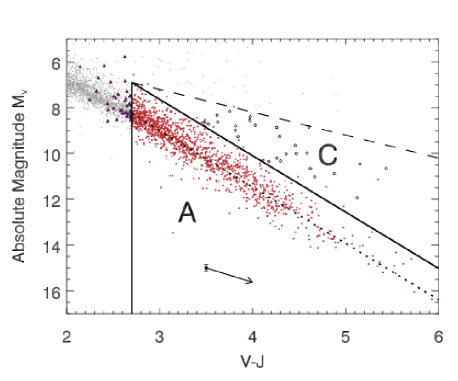
Figure 1: Selection of M dwarfs based on absolute $V$-magnitude $M_{V}$ vs. $V$-$J$ color. Red points represent “A-class” stars that are spectroscopically confirmed M dwarfs or have $V-J>2.7$ and $M_{V}$ no brighter than three standard deviations of the main sequence locus (dotted line, see Section 2 for detailed selection criteria). The upper solid curve is the main sequence locus plus three times the intrinsic width of the locus (0.46 magnitudes). The open points represent “C-class” M dwarfs that lie significantly above the main sequence but within a zone bounded by a slope one (dashed) line. This zone could be populated by stars with large errors in $V$ or $J$, binaries or very young and relatively luminous stars. Grey points represent other SUPERBLINK stars that were not selected. The point with the arrow indicates the median error in $M_{V}$ and the direction of extinction. Purple triangles are stars in the F13 catalog that were excluded from the CONCH-SHELL.

Figure 2: Selection of M dwarfs based on reduced proper motion $H_{V}$ vs. $V$-$J$ color. The symbols and lines are the same as in Fig. 1, with the addition that blue points are evolved/giant stars with $M_{V}<4.2$. “B-class” M dwarfs, represented by black points, have $V-J>2.7$, $H_{V}$ fainter than the $M_{V}$ of the main sequence locus plus an offset of +0.5 magnitudes (solid curve), and $g-r$ and $r-J$ colors consistent with M dwarfs. “C-class” M dwarfs (open points) have $H_{V}$ below the dashed slope-one line and colors consistent with M dwarfs. “D-class” M dwarfs (also open points) have reduced proper motions consistent with M dwarfs but colors inconsistent with M dwarfs. The dotted-dashed line approximately describes the maximum reddened $V-J$ that should be observed for an interloping star with unreddened $V$-$J$=2.7 and a given $H_{V}$. D-class stars in a “danger zone” to the left of this line are excluded.

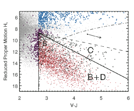
Figure 3: 2MASS $J$-$K_{S}$ color criterion for M dwarfs selected based on reduced proper motion. Symbols are the same as in Figs. 1 and 2. The dotted line is the weighted mean value ($J$-$K_{S}=0.83$) for confirmed M dwarfs. The solid lines mark $\pm$3 times the intrinsic dispersion in $J$-$K_{S}$ remaining after formal errors are subtracted (0.028 magnitudes).

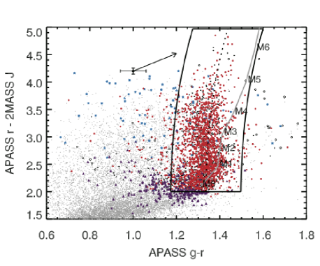
Figure 4: APASS $g-r$ vs. $r-J$ color criterion for M dwarfs selected based on reduced proper motion. Symbols are the same as in Figs. 1, 2, and 3. The dotted line is a polynomial fit to values of confirmed M dwarfs and the solid lines denote the limits $r-J>2$ and $\pm$3 times the intrinsic dispersion of the locus (0.054 magnitudes). Mean SDSS colors of M dwarfs with different spectral types from Bochanski, Hawley & West (2011) are plotted as the grey line.

3 Spectroscopy

3.1 Observations

Visible-wavelength spectra with a resolution $R=\lambda/\Delta\lambda\sim 10^{3}$ were obtained with the SuperNova Integral Field Spectrograph (SNIFS) on the University of Hawaii 2.2 m telescope on Maunakea, Hawaii, the Mark III spectrograph and Boller & Chivens CCDS spectrograph (CCDS) on the 1.3 m McGraw-Hill telescope at the MDM Observatory on Kitt Peak, Arizona, the REOSC spectrograph on the 2.15 m Jorge Sahade telescope at the Complejo Astronómico El Leoncito Observatory (CASLEO), Argentina, and the RC spectrograph on the 1.9 m Radcliffe telescope at the South African Astronomical Observatory. SNIFS acquires 3200-9700Å integral field spectra in blue and red channels that narrowly overlap at 5100-5200Å (Lantz et al., 2004). Except for metallicity determination (Section 4.2), only the red channel data were used in this project as many stars had very low signal-to-noise in the blue channel. The Mark III was used with a 1.52 arcsec slit, a Hoya yellow order-separation filter, either a 300 or 600 lines mm^-1 grating blazed at 5800Å and either the “Wilbur” or “Nellie” 2048² CCD detectors. The CCDS was used with a 158 lines mm^-1 grating blazed at 7530Å and a 1 arcsec slit, and spectra from this instrument cover 4800-8800Å. The REOSC spectrograph was used with a 300 lines mm^-1 grating blazed at 5000Å and is equipped with a $1024^{2}$ TEK CCD which is thinned and back-illuminated. The RC Radcliffe spectrograph was used with a grating having 300 lines mm^-1 blazed at 7800Å for a dispersion of 3.15Å pixel^-1 on a SITe 1024² CCD.

We obtained a total of 3071 spectra of 2583 stars or 86% of the catalog over the span of more than 11 years. 425 stars were observed twice, 14 stars were observed thrice, and 6 stars had more than four observations. A summary of the observations with each telescope/instrument combination is presented in Table 1.

3.2 Reduction

UH 2.2m and SNIFS: The majority of SNIFS data reduction was performed with the SNIFS data reduction pipeline, which is described in detail in Bacon et al. (2001) and Aldering et al. (2002). To summarize, the SNIFS pipeline performed standard CCD processing (i.e., dark, bias, and flat field corrections), and then assembled the data into two data cubes for the red and blue channels. Each data cube was then cleaned of cosmic rays and bad pixels. To mitigate errors from telescope flexure, the data were wavelength-calibrated using arc lamp exposures acquired immediately after the science exposure. The SNIFS pipeline then used a point-spread function model to estimate and subtract the background, and extract the 1D spectra from the data cube. For $\la 1$% of sources the extraction failed, usually due to the presence of a marginally resolved binary, unusually high seeing ($\geq 3$″), or a software failure. In these cases we identified the star position and extracted the 1D spectrum manually. An approximate flux calibration was applied by the SNIFS pipeline to each spectrum using an approximate instrument and atmospheric response function.

We applied an additional correction to the flux calibration using our own model. During each night we observed two to five standards with well-calibrated spectra from Oke (1990), Hamuy et al. (1994), Bohlin, Colina & Finley (1995), Bessell (1999), or Bohlin, Dickinson & Calzetti (2001). We derived an empirical wavelength- and airmass-dependent correction by comparing the spectra of all standard star observations taken over the course of the project to their spectra in the literature. We further derived a nightly term by the same technique using just the standard stars observed in a given night. However we found that the night-dependent correction was not significant on photometric nights. This method enabled us to avoid the impractical task of obtaining spectra of standards spanning the full range of observed airmasses each night. Mann, Gaidos & Ansdell (2013) found that synthetic photometry from SNIFS spectra is in excellent agreement with colors from ground-based photometry, suggesting systematic errors in the flux calibration are small. As an additional test, we compared observations of the same star on different nights. Our results suggest that random errors in the flux calibration are $\la 1$%, except around the atmospheric H₂O band at 9300-9600Å, which is known to vary on timescales shorter than those considered by our model. UH2.2m and SNIFS have been shown to be stable at the $<0.1\%$ level over the course of hours (Mann, Gaidos & Aldering, 2011), which suggests that the additional noise is coming from errors in the extraction process (see Buton et al., 2013, for a more detailed discussion).

MDM and Mark III or CCDS: Reduction of most MDM spectra were performed using the IRAF reduction package Images were de-biased and flat-fielded using the CCDPROC package. Sky emission was then subtracted, and star spectra extracted using the DOSLIT routine in the SPECRED package. Wavelength calibration was performed using arc line spectra of Ne+Ar+Xe lamps which were routinely collected after each visit on a target, to account for flexure in the spectrographs. In a small number of cases in which arc spectra were not collected immmediately after the visit, calibration was performed using the arc lamp collected on the following target, thus potentially producing small but systematic shifts. Flux calibration was performed with observations of the calibration standard stars Feige 110, Feige 66, Feige 34, and Wolf 1346 (Oke, 1990), either one of which was typically observed once every night during oberving runs. Spectra collected with the CCDS spectrograph were imaged with thin CCDs and displaying significant fringing redward of 7000Å. In this case, additional flatfields were collected immediately after each visit on a star, either just before or just after calibration arc lamps were collected. In a few instances, however, additional flatfield lamps were not collected due to overlook on the part of the observer. Flat lamps from similar H.A./Dec. pointings were used to correct for fringing, but this sometimes failed to completely eliminate the fringing patterns. As a result, weak fringing features are often seen redward of 7500Å in some spectra. MDM spectra were also occasionally found to be affected by slit losses due to our use of a relatively narrow slit and to observations conducted at large hour angles ($<$3 hours from meridian) with the slit oriented north-south of the sky and not strictly oriented along the local parallactic angle. In some cases, it was possible to determine the pattern of the slit loss based on observations of the calibration stars, and flux recalibrations were performed to correct for the losses.

We obtained spectra of several bright dwarfs to calibrate our estimates of effective temperature (Section 4.3). Some of these stars are in the CONCH-SHELL itself. These stars were reduced and calibrated using IDL scripts, rather than IRAF. Spectral images were debiased, flattened by quartz lamp flats, and the source spectrum traced by a fitting a third-order polynomial to centroid positions vs. wavelength. Cosmic ray events were identified by their effect on the along-slit width of the spectral image and filtered. Sky spectra were extracted from two flanking apertures and subtracted from the raw source spectrum. Quadratic pixel-wavelength solutions were derived from the arc lamp spectrum (Ne, Ar, and/or Xe) acquired closest in time to the target. CCDS spectra exhibit severe fringing at the red end, which required that flat fields be obtained at each pointing. This step did not entirely remove the fringes and it was necessary to identify the fringe pattern in each spectrum by Fourier transform and smoothing at the peak spatial frequency to remove the pattern. Extinction correction and flux calibration were performed using the standard KPNO extinction table and the spectrophotometric standards Feige 34, 66, and 110 (Oke, 1990).

CASLEO and REOSC: Long-slit spectra were obtained with the REOSC spectrograph by replacing the echelle grid by a mirror (see Cincunegui & Mauas, 2004). For each star we obtained two spectra to help us to remove cosmic rays. Each of the two spectra were bias corrected, optimally extracted and wavelength-calibrated using standard IRAF routines. The wavelength calibration was performed using Cu-Ar arc lamp spectra. Then we combined both spectra, removing cosmic rays. To calibrate these spectra in flux, we also observed each night at least four standard stars selected from the Catalogue of Southern Spectrophotometric Standards (Hamuy et al., 1994). The reduction and calibration were performed using standard IRAF routines.

SAAO Radcliffe and RC: Reduction of the spectra was performed closely following the prescription detailed in James (2013), with the exception that all processing was executed within the IRAF environment (Tody, 1993) instead of the Starlink one. Extracted and wavelength-corrected spectra for all targets and calibrator standard stars were corrected for local atmospheric extinction using an updated version of the Spencer Jones (1980) study. On a per night basis, extinction-corrected count rates were converted to flux by reference to the spectrophotometric flux standard star Feige 110, and its tabulated values in Massey et al. (1988) and Massey & Gronwall (1990). Flux calibration for spectra acquired on the night of UT 2013 Sept. 22 was performed using the spectrum of Feige 110 obtained on the night of Sept. 21 due to a case of mistaken identity of the flux standard observed on Sept 22.

Flux normalization: Many spectra were not obtained under conditions where absolute flux normalization was possible. Instead, all spectra were normalized to SDSS $i=0$. This band was chosen because it is mostly or entirely covered by our spectra and the emission from early M dwarfs peaks at $i$-band. For SNIFS spectra the O₂ telluric lines at $\sim 7600$Å was removed as part of our reduction, but this was not the case for most spectra obtained with other spectrographs. We derive an approximate correction to the telluric features in the remaining spectra using observations of white dwarfs or hot stars taken with the appropriate spectrograph. We assumed these stars were smooth (no features) around the O₂ atmospheric lines and therefore we measured the strength of the telluric lines by comparing the observed spectrum to one interpolated from the uncontaminated parts of the spectrum. Because telluric line strengths vary as a function of atmospheric conditions and observed airmass this correction is only approximate. After we applied the telluric correction, we convolved each spectrum with the SDSS $i$ filter transmission profile. We then integrated over the resulting spectrum, and calculated a synthetic magnitude using the zero-points from Fukugita et al. (1996). The synthetic magnitude was used to calculate a normalization constant such that the spectrum becomes that of a star with $i=0$.

4 Stellar Properties

4.1 Luminosity Class and Spectral Type

We calculated four gravity-sensitive indices at wavelengths between 6400 and 8300Å, a region covered by nearby all of our spectra (Fig. 5). These indices were (i) the averaged CaH2 and CaH3 indices (ratio of flux in bands at 6830Å and 6975Å to the continuum), (ii) the equivalent width of the K I line at 7699Å, (iii) the equivalent width of the Na I line at 8185Å, and the equivalent width of a blend of Ba II, Fe I, Mn I, and Ti I lines centered at 6500Å. Mann et al. (2012) found these indices to be effective discriminators between M dwarfs and giants with moderate-resolution spectra. We also calculated the TiO5 index, centered at 7130Å, an indicator of effective temperature for M dwarfs (Reid & Hawley, 2005). The band and continuum definitions in Mann et al. (2012) were used, with the exception of Na I (see below). Each spectrum was shifted by the offset found between its vacuum wavelength version and the rest-frame predicted spectra of a best-fit PHOENIX atmosphere model (see Section 4.3). Errors for each index were calculated by Monte Carlo simulations that included both the formal noise in each spectrum plus an assumed error in wavelength calibration with an RMS of 0.5Å. Fifty-two CASLEO/REOSC spectra were obtained with an incorrect grating setting and lack the region around H${\alpha}$ and the Ba II feature.

The four gravity-sensitive indices are plotted vs. the TiO5 index in Figs. 6-8. Stars with TiO5 index $<1$ are M-type while those with TiO5 $\approx 1$ are mostly late K stars but could include earlier spectral types as well. For each index we fit a polynomial with TiO5 to the locus and calculated the intrinsic scatter around the locus after subtracting the measurement errors. We found that the EW of the Na I doublet as defined in Schiavon et al. (1997) and used by Mann et al. (2012) produces a very large scatter, probably because the line at 8195Å and the continuum region redward of this is beyond the useful wavelength range of many of our spectra or, possibly, the presence of uncorrected telluric lines. Instead, we measured the EW of the 8183Å line in the range 8172-8197Å and only used the blue continuum region (8170-8173Å) defined in Schiavon et al. (1997). This reduced the scatter in EW, although it is still larger than that of the other lines (Fig. 9). The Na I line is especially sensitive to metallicity (Mann et al., 2013a) and this may partly explain the larger scatter.

Figure 5: Wavelength coverage of our spectra at signal-to-noise per resolution element $>20$. The locations of four gravity-sensitive indices calculated to identify interloping giant stars plus TiO5, a proxy for effective temperature, are shown.

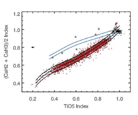
Figure 6: Mean of the CaH2 and CaH3 indices vs. TiO5 index, an indicator of effective temperature in M dwarfs. The isolated point on the left illustrates the median errors. Red points are M dwarfs confirmed by parallaxes or previous spectroscopy. The solid black lines are a least-squares polynomial fit to the M dwarf locus and plus and minus twice the intrinsic standard deviation around the locus, after subtraction of formal measurements error. Circled points are spectra where the CaH index is $>5\sigma$ above the locus, where $\sigma$ is the measurement error and intrinsic locus width added in quadrature. The blue lines are the $\pm 2\sigma$ contours for the sample of giant stars constructed by Mann et al. (2012).

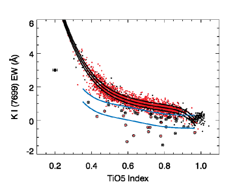
Figure 7: Same as Fig. 6 except for the equivalent width of the K I line at 7699Å.

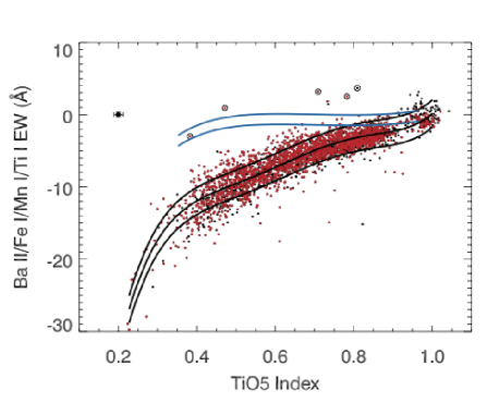
Figure 8: Same as Fig. 6 except for the equivalent width of a blend of lines of Ba II, Fe I, Mn I, and Ti I at $\sim$6500Å..

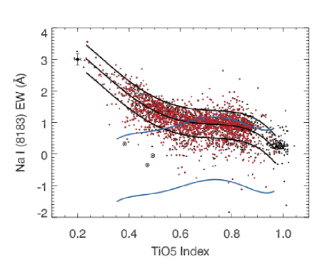
Figure 9: Same as Fig. 6 except for the equivalent width of the Na I line at 8183Å.

We flagged 39 spectra with K I, Ba II+, or CaH indices at least $5\sigma$ below the best-fit locus (circled points in Figs. 7-9). However, 20 of these are of A-class stars confirmed by parallaxes and/or spectra in Lépine et al. (2013) (red points), including some observations of very bright calibrator M dwarfs which may have entered the nonlinear response regime of the MDM Mark III detector. The majority of the flagged stars do not fall within the giant locus bounded by blue lines in Figs. 7-9, also suggesting a problem with the spectra rather than the that these are giants. The two most likely interlopers among the 39 flagged stars is the C-class star PM I13193-5800 (Tycho 8657-739-1), and one D-class star PM I06298-2250 (Tycho 6507-473-1). A SIMBAD search revealed no specific published information on any of these stars.

Fourteen of the 20 flagged spectra affiliated with A-class stars and 18 of the 19 flagged spectra belonging to B-, C- or D- class stars are flagged exclusively because of weak K I lines. Twenty-four of these were obtained with the REOSC at CASLEO and may be the product of wavelength calibration error, truncation of the spectra due to an incorrect grating setting, contamination by brighter nearby stars, or clouds. Only 10 of the flagged spectra produce a weak Ba II or CaH index, and 9 of these are A-class stars, all established M dwarfs. Some of these spectra are clearly saturated or are contaminated by much brighter, solar-type companions. One curious case is the high-proper motion M4 dwarf GJ 1218, for which all four indices are weak. This star may be metal-poor although its luminosity ($M_{V}=11.71$) rules out a subdwarf classification. The last spectrum is that of the D-class star PM I06298-2250, also with four weak indices, and it is probably of a giant: we excluded this star from the catalog.

Spectral types were determined using HAMMER (Covey et al., 2007). Because of a systematic error in the HAMMER’s automated spectral typing (Lépine et al., 2013) we used manual assignments. The distribution of spectral types is plotted in Fig. 10. We were unable to assign spectral types to 2 stars: Another 59 stars have spectra that appear to be earlier than K5. However, we could not manually assign accurate spectral types with HAMMER due to the lack of obvious spectral features, the minimal overlap between the HAMMER templates and these spectra, uncorrected slit losses, and/or other problems with the spectra. Among these 61 stars are 8 A-class stars, all of which are established M dwarfs or proper-motion stars according to SIMBAD. All of the TiO5 indices affiliated with these spectra are $>0.92$, consistent with stars earlier than M, but this does not exclude late K stars. The distributions of these objects with $V$-$J$ color and galactic latitude $b$ include a cluster at $V$-$J<3.4$ and $|b|<6$ deg. We removed all B-class stars in this cluster, as well as all C- and D-class stars among the 61 (5 stars in total). Thus we excluded a total of six stars based on their spectra, leaving 2989 stars. The overall contamination rate by giants and hotter stars before spectroscopic screening is $<$1%.

Figure 10: Distribution of CONCH-SHELL spectral types as determined by HAMMER in manual mode. An additional 18 stars in the catalog have spectra but uncertain spectral types and are not included.

4.2 Metallicity

Metallicities with respect to the solar value ([Fe/H]) were estimated following the method of Mann et al. (2013a). They used FGK+M wide binaries to identify metal-sensitive atomic and molecular features in M dwarf spectra, from which they derived an empirical calibration between the strength of these features and the metallicities of the late-type dwarf. We calculated metallicities only for CONCH-SHELL stars with SNIFS spectra. This was done because the Mann et al. (2013a) calibration utilizes at least one feature blueward of 4800Å, which is only covered by our SNIFS spectra, and because the calibration of Mann et al. (2013a) was itself derived from SNIFS spectra.

A total of 1338 stars were observed using SNIFS. We removed 100 stars because they have spectral types outside the range where the calibration is valid (K7-M5) and 53 stars because their SNR in the blue channel is too low ($<30$). We placed each of the remaining 1185 spectra in their rest frames by converting wavelengths to vacuum values then cross-correlating each spectrum to SDSS templates (Bochanski et al., 2007) of the corresponding spectral subtype. We then used an IDL routine to calculate the metallicity of each star. Errors in [Fe/H] are calculated by combining (in quadrature) measurement errors and calibration errors reported by Mann et al. (2013a).

The resulting distribution of metallicities is plotted in Fig. 11. The distribution is well described by a Gaussian centered at [Fe/H] = -0.05 with a standard deviation of 0.21 dex. The intrinsic width, after correction for measurement error, is 0.18 dex. This is consistent with previous estimates of volume-limited M dwarf samples (Johnson & Apps, 2009; Schlaufman & Laughlin, 2010), and very similar to the distribution of FGK stars in the solar neighborhood (median metallicity = -0.06, standard deviation = 0.21 dex, Casagrande et al., 2011).

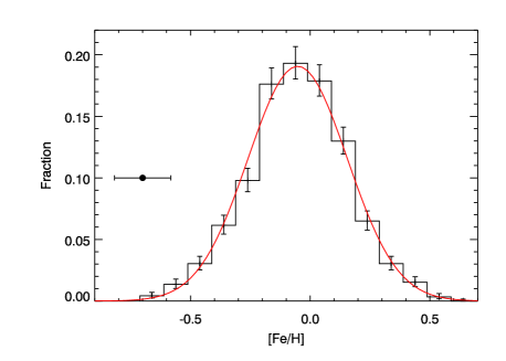
Figure 11: Distribution of metallicity among 1185 stars with spectra obtained by SNIFS. Poisson errors in each bin are shown. The lone point denotes the median error in [Fe/H] for an individual star. A best-fit gaussian is shown in red. The resulting fit is centered at [Fe/H] = -0.07 dex with a width ($\sigma$) of 0.20 dex.

4.3 Physical Parameters

To estimate the effective temperature $T_{\rm eff}$, radius $R_{*}$, luminosity $L_{*}$, and masses $M_{*}$ of these M dwarfs we followed the procedure of Mann, Gaidos & Ansdell (2013), first determining $T_{\rm eff}$ by finding the best-fit model stellar spectrum, then using the best-fit temperature in empirical relations to determine the other parameters. This procedure was calibrated on nearby stars with measured radii, distances and bolometric fluxes, and hence bolometrically-determined temperatures (Boyajian et al., 2012). Flux-calibrated, extinction-corrected spectra were compared with the predictions of the BT-SETTL version of the PHOENIX stellar atmosphere model (Rajpurohit et al., 2014). We employed the suite of models with Caffau & Freytag (2010) solar abundances. Mann, Gaidos & Ansdell (2013) showed that minimum-$\chi^{2}$ fitting of a grid of models and their interpolations recovered the bolometric temperatures of M dwarfs with an accuracy of 60 K.

We followed the procedure of Mann, Gaidos & Ansdell (2013), with a few modifications. We excluded the same set of wavelength intervals where the models perform poorly to improve the fit. The observed and model spectra are normalized by their median values, and a uniform wavelength offset between them is allowed as a free parameter of the fit. However, we introduced a third-order polynomial with wavelength to represent slit loss: the coefficients are free parameters and are not interpreted. We also added a quadratic term with model [Fe/H] to the $\chi^{2}$ used to describe the goodness-of-fit of a model, i.e. $({\rm[Fe/H]-[Fe/H]}_{0})^{2}/\sigma_{\rm[Fe/H]}^{2}$. For fits to SNIFS spectra where the stellar metallicity was determined (Section 4.2), [Fe/H]₀ is the measured value and $\sigma_{\rm[Fe/H]}^{2}$ is the measurement uncertainty. For fits to other spectra, we substituted the mean and standard deviation of all SNIFS values of [Fe/H]. To more thoroughly explore the range of possible spectra, 10000 interpolations were generated from sets of three rather than two normalized spectra. The interpolations draw from the best-fit (minimum $\chi^{2}$) model spectrum and at least 6 other model spectra with the lowest $\chi^{2}$, up to $\chi^{2}_{min}\left(1+\Delta\chi_{\nu}^{2}\right)$, where $\Delta\chi_{\nu}^{2}$ is the increase in the reduced $\chi^{2}$ corresponding to the 95% confidence interval. After the best fit of these interpolations was identified, we estimated the error in $T_{\rm eff}$ calculated as one-fourth the 95% confidence interval in $\chi^{2}$. We added 60K in quadrature to this error to represent the accuracy of our calibration.

For each best-fit model we calculated the associated quantity $\epsilon=\sqrt{\chi_{\nu}^{2}-1}/{\rm SNR}$, an estimator of the mean error in excess of formal error due to observational systematics and imperfect modeling of the stellar spectrum. Values of $\epsilon$ are plotted vs. the best-fit $T_{\rm eff}$ in Fig. 12. The locus of points at low $\epsilon$ are dominated by SNIFS spectra, with systematic errors as low as $\sim$1%. This locus rises with decreasing $T_{\rm eff}$ as the imperfectly-modeled molecular bands of M dwarf spectra become more pronounced and contribute more to $\chi^{2}_{\nu}$.

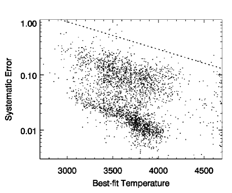
Figure 12: Systematic error $\epsilon$ of the best-fit of PHOENIX BT-SETTL model to stellar spectra vs best-fit $T_{\rm eff}$. Fits with $\epsilon$ above the dashed line were not used to calculate stellar parameters.

Forty-one spectra with $\epsilon$ above the dashed line in Fig. 12 and/or best-fit wavelength offsets exceeding the spectrograph FWHM, indicating a problem with fitting or wavelength calibration, were not used to estimate $T_{\rm eff}$. An offset exceeding 5.4Å, the highest spectral resolution in our survey, corresponds to a radial velocity of 250 km sec^-1, something exceedingly unlikely to be observed in our sample. Some CASLEO spectra were obtained with an improper grating setting and that limited the range of usable wavelengths. Others were obtained at high airmass or on cloudy nights, with low signal-to-noise, or suffered contamination by twilight or a nearby full Moon. If more than one acceptable value of $T_{\rm eff}$ was available a weighted mean was used.

Mann, Gaidos & Ansdell (2013) calibrated this method of obtaining $T_{\rm eff}$ using spectra obtained with SNIFS. The same analysis of spectra obtained with other instruments may introduce systematic differences between the best-fit temperatures and the bolometric temperatures. To determine such offsets we observed several of the Boyajian et al. (2012) calibrator stars having $T_{\rm eff}$$<4200$ K with each telescope/instrument combination. The comparisons between best-fit and bolometric temperatures are shown in Fig. 13. We calculated the weighted mean offset for each instrument: an F-test using the ratio of variances showed that fitting a line with a non-unit slope did not significantly improve the fit. The offsets ($T_{\rm bol}-T_{\rm fit}$) were $40\pm 26$K for the Mark III at MDM, $42\pm 21$K for the CCDS at MDM, $25\pm 42$ for the CASLEO/REOSC spectrograph, and $18\pm 24$ for the SAAO Radcliffe 1.9m/RC spectrograph. Spectra for most of the stars in the northern hemisphere were previously analyzed and temperatures estimated by the same process of model fitting (Lépine et al., 2013) but using BT-SETTL models with the Asplund et al. (2009) abundances. Our revised temperatures using the new PHOENIX models are systematically 100-150K hotter, as was previously noted by Mann, Gaidos & Ansdell (2013).

Models of the spectra of M dwarf stars, particularly the TiO and CaH lines, have significantly advanced, but challenges remain (Rajpurohit et al., 2014). Discrepancies between the models and the actual spectra of stars will (i) inflate contribution of the spectral contributions to $\chi^{2}$ relative to other measurements such as [Fe/H] and (ii) bias stellar parameters from least-$\chi^{2}$ fits toward the direction of more reliable stellar models, not necessarily more accurate parameters. The trend of increasing systematic error with decreasing $T_{\rm eff}$ in Fig. 12 raises the spectre of a bias in best-fit $T_{\rm eff}$ towards higher temperatures where the PHOENIX models are more accurate. However, the excellent agreement between best spectral fit temperatures and bolometric temperatures of our calibrator stars (Fig. 13) indicates this effect is small, perhaps limited by the deep features in the spectra of late M dwarfs.

Figure 13: Stellar $T_{\rm eff}$ of calibrator stars from least-squares fitting of PHOENIX models to spectra obtained with four instruments on three telescopes. These values are compared to bolometric temperatures determined from measurements of angular radii and bolometric fluxes. The dotted line is equality and the dashed line is a minimum $\chi^{2}$ fit. The weighted-mean offset is reported in each panel.

If no value from acceptable spectral fits was available, we calculated $T_{\rm eff}$ based on $V$-$J$ color and a best-fit polynomial for $T_{\rm eff}$ vs. $V$-$J$ (Fig. 14): $T_{\rm eff}=4068.8-916.1\left(V-J-2.7\right)+956.8\left(V-J-2.7\right)^{2}-868.0\left(V-J-2.7\right)^{3}$. The uncertainties in these values are derived by adding in quadrature the uncertainties from error in $V$-$J$, the intrinsic scatter of the locus (40 K), and the uncertainty in the zero point of the spectroscopic $T_{\rm eff}$ calibration (43 K, Mann, Gaidos & Ansdell, 2013). A number of stars yield spectral best-fit $T_{\rm eff}$ values that are significantly hotter than their $V-J$ colors; these conflicts may be the result of blends with brighter stars (affecting photometry) but also inaccuracies of spectral fits at $T_{\rm eff}$$>4200$K where there are no broad molecular features. For cases of the latter kind we replaced the spectroscopic $T_{\rm eff}$ with values based on $V-J$. Nineteen D-class stars with $V-J>6$, beyond the valid range of our fit — and the plausible range of bright M dwarfs — were excluded. We retained one M dwarf with $V-J>6$ (GJ 1230B or PM I18411+2447N), but did not assign a value of $T_{\rm eff}$. Our final catalog contains 2970 stars.

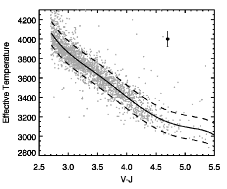
Figure 14: Stellar $T_{\rm eff}$ of stars from least-squares fitting of PHOENIX models vs. $V$-$J$ color. The single point with the error bars represents median uncertainties in $V$-$J$ and $T_{\rm eff}$ (91K). The curve is the weighted least-squares fit of a third-order polynomial and is used to estimate the $T_{\rm eff}$ of stars without spectra or acceptable PHOENIX model fits. The dashed lines represent $\pm$ twice the intrinsic width of the locus (40K) in $T_{\rm eff}$ after accounting for formal errors.

The distribution of the estimated $T_{\rm eff}$ values of CONCH-SHELL stars is plotted in Fig. 15 and included in Table 2. The nearly total absence of stars cooler than $T_{\rm eff}$ $\sim 3000$K is a result of the magnitude limit of the catalog. The appearance of stars hotter than $T_{\rm eff}$ $\sim 4000$K reflects the dispersion between stellar colors and $T_{\rm eff}$ and the inclusion of late K dwarfs in this catalog, plus errors exceeding 100 K for many stars.

We estimated stellar radius $R_{*}$, luminosity $L_{*}$, and mass $M_{*}$ using the metallicity-independent empirical relations of Mann, Gaidos & Ansdell (2013). Our calibration is only valid for $T_{\rm eff}$$>$3238K. For cooler stars we report upper limits based on $T_{\rm eff}$ = 3238K. These values are reported in Table 2. Errors were calculated by combining, in quadrature, the formal errors from the uncertainty in $T_{\rm eff}$ and the uncertainties in the empirical calibration.

Figure 15: Distribution of stellar $T_{\rm eff}$ in the CONCH-SHELL catalog. Values for stars without acceptable spectra are based on $V$-$J$ color.

4.4 Comparison of Parallax- and Spectroscopy-Based Luminosities and Masses

For some stars we have parallaxes which, along with a bolometric correction, allowed us to independently determine luminosities and estimate masses from a mass-luminosity relation. We constructed a bolometric correction to the $J$-band magnitudes of M dwarfs using the parameters in Mann, Gaidos & Ansdell (2013) and an analysis of 23 K and early M interferometry targets in Boyajian et al. (2012). A quadratic function in $V$-$J$ color was fit to the BC values and the best-fit polynomial was found to be ${\rm BC}=0.69+0.44\left(V-J\right)-0.037\left(V-J\right)^{2}$, with a scatter of only 0.03 magnitudes. This was applied to 1068 CONCH-SHELL stars with Hipparcos parallaxes to calculate luminosities. We estimated masses from the absolute $K$ magnitudes and the mass-luminosity relation of Delfosse et al. (2000).

We compare spectroscopic-based luminosities to trigonometric values, both in solar units, in Fig. 16. Figure 17 compares estimates of stellar mass. All sources of formal error, including that from the bolometric correction, are included. The weighted mean difference (spectroscopic - trignometric) between the logarithmic luminosities is $0.082\pm 0.003$ dex. The average $\chi^{2}$ is 3.6 and 24 stars are more than 5$\sigma$ away from the line of equality (circled points). This is almost certainly the result of (i) underestimation of the errors in $T_{\rm eff}$ and the sensitivity of our luminosity esstimates to $T_{\rm eff}$; (ii) spectroscopic undersestimates of $T_{\rm eff}$ and $L_{*}$ for late K stars where there are few informative features in medium-resolution spectra. The empirical relations of Mann, Gaidos & Ansdell (2013) are valid only for main-sequence, inactive stars and highly active and/or very young stars may contribute to the dispersion. Removing stars with H${\alpha}$ in emission (see Section 4.5) slightly reduces the number of $5\sigma$ outliers and mean $\chi^{2}$.

We compare spectroscopic masses to those based directly on parallaxes and $K$ magnitudes in Fig. 17. The weighted mean fractional difference (spectroscopic-parallax) is -6.3$\pm$0.9% and the mean $\chi^{2}$ is 0.69. Figures 16 and 17 are not independent because the empirical curves from Boyajian et al. (2012) and Mann, Gaidos & Ansdell (2013) are based on a mass-luminosity relation (Henry & McCarthy, 1993). Users of CONCH-SHELL may wish to substitute masses and luminosities based directly on absolute $K$-magnitudes and a mass-luminosity relation for those stars with parallaxes.

Figure 16: Luminosities (solar units) based on best-fit $T_{\rm eff}$ and the empirical relations in Mann, Gaidos & Ansdell (2013) compared to values calculated from Hipparcos parallaxes, $J$-band magnitudes, and a bolometric correction. The point with error bars indicates the median uncertainties.

Figure 17: Masses (solar units) based on best-fit $T_{\rm eff}$ and the empirical relations in Mann, Gaidos & Ansdell (2013) compared to values calculated from Hipparcos parallaxes, $K$-band magnitudes, and the mass-luminosity relation of Delfosse et al. (2000). The point with error bars indicates the median uncertainties.

4.5 Activity: H$\alpha$ Emission

The equivalent width of H${\alpha}$ was calculated by shifting each spectrum to the rest frame using the wavelength offset produced when matching our spectra to the PHOENIX model atmospheres (Section 4.3). Following Lépine et al. (2013), the 14Å-wide spectral region between 6557.61 and 6571.61Å (in air) was used to compute the EW of H${\alpha}$, and 6500-6550Å and 6575-6625Å regions were used to compute the continuum. Errors were calculated using the Monte Carlo method assuming Gaussian-distributed noise and random wavelength calibration errors with an RMS of 0.5Å. Values of EW are plotted vs. the TiO5 index in Fig. 18. Inactive stars with no H${\alpha}$ emission have negative EW values because of the spectral slope between the H${\alpha}$ region and the continuum regions. We fit a quadratic function with wavelegnth to these values and calculated the intrinsic width of the locus to be 0.42Å after subtracting formal errors. Significant ($3\sigma$) emission is seen in 404 stars or about 13% of stars with spectra that cover the H${\alpha}$ region, and there is a marked increase in the envelope of EW values towards cooler temperatures or later spectral types, as expected (e.g., Stassun et al., 2011).

The 13% active fraction and the trend with spectral type are consistent with previous studies of M dwarf activity (e.g., West et al., 2008; Gizis et al., 2000), which find typical active fractions for early-M dwarfs (M0-M3) to be $\sim$10%. However, this active fraction significantly increases for later spectral subtypes, reaching $\sim$30% by M4 and >80% by M7. Moreover, West et al. (2008) showed that the active M dwarf fraction decreases with vertical distance $z$ from the galactic plane, e.g., for M3 dwarfs, $\sim$40% at 25 <$|$z$|$<50 pc compared to $\sim$10% at 150 <$|$z$|$<175 pc). Our intermediate value reflects the opposing influences of the dominance of late K and early M dwarfs over mid-M dwarfs in the CONCH-SHELL catalog (Fig. 10), which have a lower active fraction, and the bias towards nearby stars which are close to the galactic plane and have a higher active fraction.

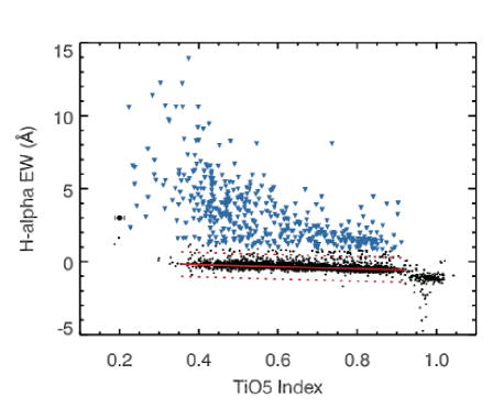
Figure 18: H${\alpha}$ equivalent width vs. TiO5 index. Blue points are spectra of stars with significant ($3\sigma$) emission. A few stars with TiO5 $\sim 1$ (stars with late K or even earlier spectral types) appear to show H$\alpha$ in absorption.

4.6 Multiplicity

The SNIFS image cubes provide spatial information that can be used to search for binaries. SNIFS image cubes cover $6\times 6$ arcsec fields of view with 0.4 arcsec pixels (Aldering et al., 2002; Lantz et al., 2004). This limited number of pixels and low spatial resolution prohibited the use of Gaussian source finders to identify companions. Instead, a principal component analysis of the two-dimensional, white-light version of the SNIFS image cubes and by-eye checks were used to identify binaries. The principal axes were calculated as the eigenvectors of the spatial image moment of the background-subtracted image. Only pixels that were above a certain threshold multiple of the image noise were used, where the threshold multiple scaled with the signal-to-noise of the image. An elongation factor $E$, the ratio of the square root of the principle moments, and the rotation angle $\theta$ between the principal axes and the EW-NS image coordinate system were used as parameters to identify candidate binaries. Criteria for $E$ and $\theta$ were set by average values from populations of single, binary, and elongated sources identified by eye. Candidate binaries are those with: $E>1.16$ for any $\theta$ or $1.03<E<1.16$ and $\theta<75^{\circ}$. These complex criteria are imposed because telescope tracking errors tend to elongate images of point sources in the E-W direction. This analysis was applied to 1207 SNIFS image cubes to identify 499 candidate binaries, then by-eye inspection of the candidates confirmed 71 resolved binaries, i.e a rate of $5.9\pm 0.7$%.

Given the spatial resolution and field of view of SNIFS, which restricts resolvable binary separations to $\sim$1.5–4.5 arcsec, a 5.9% binary rate is consistent with previous studies of M dwarf multiplicity . One of the largest M dwarf multiplicity studies to date is AstraLux (Janson et al., 2012), which included late-K to late-M dwarfs. The AstraLux survey found 48 binaries out of 761 systems within this separation range. This $6.3\pm 0.9$% rate is perfectly consistent with the rate we find among CONCH-SHELL stars.

5 Comparison with the Frith et al. Catalog

Frith et al. (2013, F13) constructed a catalog of 8479 bright ($K_{S}<9$) M dwarf candidates selected from the PPMXL proper motion catalog (Roeser, Demleitner & Schilbach, 2010) on the basis of reduced proper motion and USNO-B photographic BRVI and 2-MASS $JHK_{S}$ colors. The F13 catalog is most similar to CONCH-SHELL in terms of source catalog and selection criteria, and, because all M dwarfs have $J$-$K_{S}>0$, we can compare the two by imposing a $J<9$ cut on F13. The F13 cut in $V$-$J$ color is identical to ours ($>2.7$), although they imposed additional (but not necessarily independent) color cuts with $B-R$, $B$-$I$, $R$-$I$, and $I$-$J$ colors. Their cuts in $J$-$H$ and $H$-$K_{S}$ colors are not equivalent to ours but have a similar outcome, selecting stars with $J$-$K_{S}$ between $\approx 0.7$ and $\approx 1$. To separate dwarfs from evolved stars, F13 impose a uniform reduced proper motion criterion $H_{K}>6$. Given that M dwarfs have $J$-$K_{S}>0.65$, this criterion is approximately equivalent to $H_{J}>6.65$, and hence $H_{V}>6.65+V-J$. At $V-J=2.7$ their cutoff in $H_{V}$ is about 0.5 magnitudes fainter and hence more conservative than ours. By $V$-$J$=5 the $H_{V}$ criterion of F13 is nearly three magnitudes brighter (more relaxed) than ours, the result of F13 using a color-independent criterion for $H_{K}$ and thus neglecting variation in absolute magnitude $M_{K}$ along the main sequence. However, our selection of C-class candidates (open points in Fig. 2) approximates their criterion because the dashed line in Fig. 2 represents a constant $H_{J}=6.15$. Another difference between F13 and CONCH-SHELL is that the former excluded stars within 15 deg. of the galactic plane, and slightly farther away at the longitude of the galactic center.

Of the 3027 F13 stars with $J<9$, 178 do not have a match in CONCH-SHELL within 2.5 arcsec. Of these, 48 show no detectable proper motion ($\mu<10$ mas yr^-1) in either the Palomar plate data or the Naval Observatory Merged Astrometric Dataset (Zacharias et al., 2005). These may be artifacts in the PPMXL catalog. Another 79 stars have $\mu$ below the formal completeness limits of the SUPERBLINK catalog (40 mas yr^-1 in the north, 150 mas yr^-1 in the south) and another 8 have $\mu<50$ mas yr^-1. This leaves 43 Frith stars that were missed by SUPERBLINK: 39 are in the south. SIMBAD searches at the locations of the 43 reveal most to be nearby late K or M dwarf stars.

Of those F13 stars that do have SUPERBLINK matches, 306 are not in CONCH-SHELL. Of these, 237 have revised (APASS-based) $V$-$J$ colors that are too blue ($<2.7$). These include many late K stars but also some very early M-type dwarfs, the inevitable result of a catalog selected by color rather than spectral type. Fifty-five other stars have $M_{V}$ or $H_{V}$ that are too bright. Of the remaining 14 stars, one is excluded by its parallax, two by proper motions, and 11 by colors inconsistent with M dwarfs and their location in the “danger zone” of the $H_{V}$ vs. $V$-$J$ diagram where extincted interlopers may be a problem. Among CONCH-SHELL stars, 474 are not in F13. More than half of these (249) are at $|b|<15^{\circ}$ which F13 does not cover. There are 338 of the best candidates (class A and B) that are not in F13.

6 Expected Yields from Exoplanet Surveys of CONCH-SHELL Stars

We calculated the yield of future transit and Doppler surveys for exoplanets around stars in the CONCH-SHELL catalog using an inference of the planet population orbiting late-type ($T_{\rm eff}$ $<$ 4200 K) Kepler stars. Although the solar-type stars observed by Kepler lie at kpc distances, the few thousand M dwarfs in the target catalog are at most a few hundred pc away and well within the galactic “thin disk” population (Gaidos et al., 2012). The metallicity distribution of Kepler M dwarfs is also similar to that in the Solar Neighborhood (Mann et al., 2013b). Kepler observations were significantly more sensitive than the expected performance of TESS and the duration of those observations more than four times longer, thus this method is not limited by Kepler incompleteness. Likewise, transit surveys such as Kepler are generally more sensitive to small, rocky planets than Doppler surveys because of signals in the former scale with planet radius as $R_{p}^{2}$, while those in the latter scale as $R_{p}^{4}$ (Sotin, Grasset & Mocquet, 2007). The derivation of the planet population and its distribution with radius and orbital period are presented in the Appendix. Briefly, we found that M dwarfs host an average of 2 planets with radius of 0.5-6$R_{\oplus}$ and orbital period $P<180$ d. The distribution with radius peaks at $\sim 0.8$$R_{\oplus}$ and the distribution with orbital period follows a power-law with index 0.66 (Figs. 21-22).

6.1 Transiting Exoplanet Survey Satellite

We predicted detections of planets around CONCH-SHELL stars by the Transiting Exoplanet Survey (TESS) mission (Ricker et al., 2010). To simulate the potential yield of TESS observations, the entire synthetic Kepler population was placed around 1000 Monte Carlo replicates of each CONCH-SHELL star in which $T_{\rm eff}$, $M_{*}$, $R_{*}$, and $L_{*}$ were drawn from Gaussian distributions with the standard deviations as calculated in Section 4.3. For each planet, the probability of a transiting orbit was calculated assuming isotropically-distributed inclinations, Rayleigh-distributed eccentricities (mean of 0.2), and uniformly distributed argument of periastron.

The number of transits observed by TESS was drawn from a Poisson distribution with a mean of $T/P$, where $T$ is the observation time. The observation time was found by reconstructing TESS sky coverage based on Fig. 7 in Ricker et al. (2014). The reconstruction consists of 104 pointings each covering $24\times 24$ deg with dwell times of 27 days. The pointings are evenly and symmetrically distributed between the northern and southern ecliptic hemispheres in 26 pairs of 4 pointings each at 13 ecliptic longitudes spaced uniformly with ecliptic longitude starting at 26.6^∘ and ecliptic latitudes (north or south) of 18, 42, 66, and 90^∘.

Transit durations were calculated using the distribution of dimensionless duration values $\Delta$ described in the Appendix. The noise during a single transit observation was calculated assuming a pure photon noise contribution of 190 ppm for an $i=11$ star over 1 hr plus 60 ppm of fixed systematic noise, added in quadrature. The detection threshold was set to SNR $>12$, a level where the Kepler false-positive rate is very low (Fressin et al., 2013). For detected planets we also calculated the orbit-averaged stellar irradiation as in terrestrial units $L_{*}/4\pi a^{2}$, ignoring the small effect of a non-zero eccentricity.

We calculated the fraction of planets detected by averaging over all Monte Carlo replicates of each star and multiplying by the total occurrence $f=2$. We calculated the stellar irradiation in terrestrial units using $S=L_{*}(P/365.24\,{\rm d})^{-4/3}M_{*}^{-2/3}$ and we ascertained whether planets orbit in the habitable zone described by the $T_{\rm eff}$-dependent “runaway” and maximum CO₂ greenhouse limits on $S$ proscribed in Kopparapu et al. (2013).

We estimate that TESS will observe 87% of CONCH-SHELL stars and that it will find $\sim 17$ planets, with only a 1.3% chance of finding a planet in the habitable zone of one of these stars. If the detection threshold is relaxed to SNR$>7.1$, the predicted number of detections rises to 26.6, but at the expense of an elevated chance of including false positives. Figure 19 show the distribution of predicted TESS discoveries with planet radius, peaking at 2$R_{\oplus}$ and falling precipitously by 1$R_{\oplus}$. We find that the star most likely to have a detectable planet is PM I19074+5905 (LSPM J1907+5905), at 2.2%. It is a mid-M type star with a comparatively small radius located close to the ecliptic pole where observations by TESS will be nearly continuous.

TESS detections of planet around CONCH-SHELL stars, especially planets in habitable zones, is limited by the short observing intervals and biased toward short-period orbits, where, according to Kepler statistics, there are fewer planets (Fig. 22). It is also limited by higher photometric noise compared to Kepler and the rapid decline in M dwarf planet population with increasing radius (Fig. 21). The distribution of simulated detections with the $T_{\rm eff}$ of the host star increases with cooler $T_{\rm eff}$, peaking at $\sim 3500$K. Cooler stars have smaller radii and planets produce larger transit depths, but they also tend to be fainter, and observations have higher noise. Assuming the M dwarf planet population does not depend on host star mass, the balance between these trends in ideal surveys favors lower $T_{\rm eff}$. Below 3500K, predicted TESS detections fall; some of this is due to the $T_{\rm eff}$ distribution of the magnitude-limited CONCH-SHELL catalog itself (Fig. 15). However, the distribution of detections per star also turns over at about 3300K, or spectral types M3-M4, suggesting that the pursuit of even cooler stars may not be very profitable. The $i$-magnitude limit of CONCH-SHELL is about 10.5 at the K-M dwarf boundary, thus there are additional, fainter stars with these spectral types which could be included, but of course these will be less attractive targets for follow-up. An extended TESS mission consisting of a single set of four $24\times 24$ deg. fields will detect many more systems per star, but for fewer stars. A few of the largest planets might even be detectable by ground-based surveys such as MEarth (Berta et al., 2012).

Figure 19: Predicted distribution of radius of planets detected at SNR $>12$ by TESS around CONCH-SHELL stars. The total number of expected detections is $\sim$17.

6.2 Infrared Doppler Radial Velocity Survey

We simulated the yield of a hypothetical Doppler radial velocity survey of a subset of these M dwarfs, such as those proposed for the CARMENES (Quirrenbach et al., 2012), Habitable Planet Finder (Mahadevan et al., 2012), IRD (Tamura et al., 2012), or SPIRou (Thibault et al., 2012) infrared spectrographs. We assumed the following survey parameters: (i) 300 survey nights over 5 years; (ii) 10 minute integration per measurement plus two minutes overhead and calibration and thus observations of 50 stars per night, or 15,000 observations. We assumed combined measurement error and photosphere “jitter” of 2 m sec^-1. These parameters are similar to proposed surveys but we do not attempt to replicate any specific survey. Extensive numerical simulations have shown that for systems with a single dominant planet, $\sim$11 radial velocity measurements are sufficient to identify a Keplerian signal with high confidence and distinguish it from stellar “jitter” (false positive probability of $<1$%) (Fischer et al., 2012). At the level of Earth masses many stars may host multiple planets (e.g. $f=2$ above) and disambiguation of the measurements into separate signals requires many more measurements, of order $\geq$50 (e.g. Fischer et al., 2012). Thus we assume 50 measurements on each of 300 stars.

We used the same planet population constructed from the Kepler sample described in Section 6.1. To translate planet radii into masses, we employed two different mass-radius relations. While the mass-radius relations for rocky planets is roughly $M_{p}\sim R_{p}^{4}$, there is tentative evidence that planets larger than $\sim 1.5$$R_{\oplus}$ have thick gas envelopes that contribute significantly to their radii (Marcy et al., 2014; Hadden & Lithwick, 2013). The two relations are $M_{p}\sim R_{P}^{2}$, a scaling which connects Earth, Neptune, and Saturn, and implies increasing gas content with planet radius/mass (Lissauer et al., 2011), or $M_{P}\sim R_{P}$ as found by Weiss & Marcy (2014) over the range 1.-5-4$R_{\oplus}$. The actual planet population around M dwarfs undoubtedly consists of a mix of objects (Gaidos et al., 2012; Wolfgang & Laughlin, 2012) that cannot be represented by a single mass-radius relation. We use the two cases of $M_{p}\sim R_{P}^{\gamma}$, where $\gamma=1$ and $\gamma=2$, to bracket the possible planet yields of Doppler surveys.

We constructed a $1000\times$ Monte Carlo representation of the CONCH-SHELL catalog and placed 50,000 randomly drawn planets around an equal number of randomly drawn Monte Carlo stars. Orbital inclinations, eccentricities, and phases were drawn from isotropic, Rayleigh (mean of 0.2), and uniform distributions, respectively. We assumed Gaussian-distributed per measurement error with RMS of 2 m sec^-1. Our detection criterion is minimalist: power in a periodogram close to the true period with a false alarm probability $p<0.01$, calculated using an implementation of the method of Scargle (1982) by Horne & Baliunas (1986). The dependence on mass-radius relation is substantial: the “heavy” mass-radius relation ($\gamma=2$) leads to a prediction of 32 detections with a peak at around 5$M_{\oplus}$ (Fig. 20) while the “light” relation ($\gamma=1$) predicts only 7 detections with a peak at $\sim 2$$M_{\oplus}$. The predicted numbers of detections in the habitable zone between the runaway and maximum CO₂ greenhouse conditions, are 3.5 and 0.4, respectively.

These contrasting outcomes demonstrate the sensitivity of such predictions to the mass distribution of small planets about which, unlike the radius distribution, we know very little. On a more positive note, combining Kepler transit and Doppler radial velocity data on separate samples is one method of investigating the mass-radius of small planets (Gaidos et al., 2012; Wolfgang & Laughlin, 2012), at least to the extent that the populations around the two sets of stars are statistically the same. Of course, Doppler observations of the transiting planets discovered by TESS should prove a more direct way of investigating the nature of these worlds.

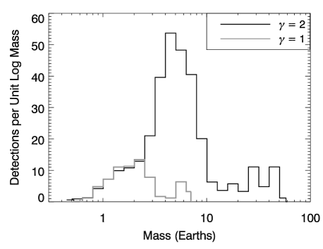
Figure 20: Predicted mean mass distribution of planets detected around 300 CONCH-SHELL stars by a hypothetical infrared Doppler radial velocity survey. The planet population is that inferred around Kepler M dwarfs and two different mass-radius relations of the form $M_{P}\sim R_{P}^{\gamma}$ are used. The total numbers of detections are 7 ($\gamma=1$) and 32 ($\gamma=2$).

7 Summary and Discussion

We have constructed a catalog of 2970 of the brightest late K and early M dwarfs on the sky. These stars were selected on the basis of parallaxes or proper motions, and visible and infrared colors. They will be among the most suitable targets for searches for Earth- to Neptune-size planets by future space photometry missions and ground-based infrared Doppler surveys. Importantly, the bright host stars of such planets will be amenable to follow-up observations, e.g. spectroscopy during transits and secondary eclipses by the James Webb Space Telescope and a future generation of extremely large ground-based telescopes. We provide three data products with this manuscript: a minimal catalog of essential stellar parameters established for all stars and useful for selecting stars for follow-up and exoplanet surveys (Table 2); a full catalog with all available parameters and their uncertainties (online machine-readable Table 3); and a data structure containing a spectra for each CONCH-SHELL star that was observed.

To select very cool dwarfs and screen giants and hotter stars we applied four sets of criteria (A-D, in decreasing order of rigor). We obtained spectra of about 86% of the catalog which we used to eliminate 44 evolved or hotter stars. We estimate that the rate of contamination in the unscreened part of the catalog is 0.23%, although this rate may be higher among “D-class” stars. We determined the metallicity of 1250 stars with spectra and find a mean of [Fe/H] of -0.07, similar to previous estimates for M dwarfs in the solar neighborhood. For about 13% of the stars the Balmer H${\alpha}$ line is seen in emission and there is an increase in both occurrence and equivalent width for later, cooler stars. In addition to assigning spectral types, we fit PHOENIX BT-SETTL model spectra to determine effective temperatures and use empirical relations to estimate stellar radii, luminosities, and masses.

We estimated the number of planets that should be discovered around these stars by the NASA TESS mission. We based our calculations on the planet population inferred to orbit Kepler M dwarfs. We estimate that about 17 planets will be detected at SNR $>12$. The number grows to 26 if the SNR criterion is relaxed to 7.1 (the nominal detection threshhold of Kepler). The radius distribution peaks at $\sim$2$R_{\oplus}$ and only 1-2 Earth-size planets are expected. Assuming the planet population is uniform with respect to $T_{\rm eff}$, most planets will be found around stars with $T_{\rm eff}$$\sim 3500$K (spectral type M2). We also estimated that an infrared Doppler survey of 300 of these stars over 300 nights will discover between 7 and 32 planets, depending on the mass-radius relation for planets smaller than Neptune. The expected yield of planets in circumstellar habitable zones is 0.5-3.5 from the Doppler survey, but essentially none from TESS, a consequence of the stronger bias of transit surveys towards short-period orbits.

Because of selection based on proper-motion and parallaxes, our catalog is not complete to $J<9$. Kinematic bias and completeness were considered for the northern sky in Lépine et al. (2013), who estimated that about 95% of M dwarfs to $J<9$ were captured by the SUPERBLINK catalog. The southern proper motion completeness limit is considerably higher ($\sim 150$ mas yr^-1) and thus is expected to be less complete. We revisited this calculation using the transverse velocity distribution of Hipparcos stars within 100 pc (van Leeuwen, 2007), the $J$-band luminosity function of Cruz et al. (2007) and considering stars with $M_{J}>5$ (Lépine et al., 2013). We find the completeness in the northern sky to be 98.6%, that in the souther sky to be 88.4%, and the coverage-weighted kinematic completeness for the survey to be 95.2%. We estimate that about 152 M dwarfs were missed due to kinematic incompleteness of the SUPERBLINK catalog. This figure is similar to the 130 M dwarf candidates selected by Frith et al. (2013) from the PPMXL catalog that exhibit detectable proper motion but were missed by in the SUPERBLINK input catalog. Two other sources of SUPERBLINK incompleteness arise from saturation of the source photographic plates in the proximity of very bright stars, as well as saturation of the cores of stars of interest, which hinder accurate astrometry (Lépine et al., 2013). Our catalog is also constructed based on $V$-$J$ color rather than spectral type, and some M0 stars with blue colors, e.g. metal-poor stars, are omitted (Lépine & Gaidos, 2011). As an experiment, we removed the $V$-$J>2.7$ color criterion, but imposed the requirement that the absolute $J$ magnitude $M_{J}>5.46$, the value of the best-fit main sequence locus at $V$-$J$=2.7. This added 342 stars, presumably a mixture of late K and M0 spectral types, to the class A sample, an augmentation of nearly 18%.

We did not obtain spectra of 412 CONCH-SHELL stars and we encourage community involvement to complete the spectroscopic survey. The AAVSO expects to release two more versions of the APASS photometric catalog: DR8 will improve photometry in the northern sky, and DR9 will re-analyze the entire catalog (A. Henden, pers. comm.). Refined photometry can be used for improved selection of M dwarfs as well as to flux-calibrate existing spectra. The Gaia satellite, launched in December 2013, will obtain parallaxes with a precisions of about 10 $\mu$as (de Bruijne, 2012) thus allowing extremely precise determination of distance modulus. Measurements of bolometric flux and effective temperature could be combined to determine radii. These stars can also serve as a source catalog for studies other than exoplanets, e.g. the ultraviolet (UV) emission from active, potentially young M dwarfs and the UV luminosity function (Ansdell et al. in prep.)

Table 1: Telescopes & Instruments Used to Obtain Spectra

Telescope	Latitude	Longitude	Instrument	FHWM (Å)	Spectra	UT Dates
MDM/McGraw-Hill	31.95173 N	111.61664 W	Mark III	5.4	1098	2002/06/22- 2013/10/25
MDM/McGraw-Hill	31.95173 N	111.61664 W	CCDS	5.4	113	2011/06/17- 2013/10/14
MKO/UH 2.2m	19.82303 N	155.46937 W	SNIFS	6.5	1338	2009/02/22- 2014/02/24
SAAO/Radcliffe 1.9m	32.46127 S	20.81167 E	RC Spec.	7.4	150	2013/09/18- 2013/09/25
CASLEO/Sahade 2.15m	31.79917 S	69.30333 W	REOSC	13.9	372	2010/09/11- 2013/10/29

Table 2: CONCH-SHELL Catalog (Minimal)

SUPERBLINK	RA (J2000)	Dec (J2000)	V	J	d	Class	SpT	[Fe/H]	$T_{\rm eff}$	$R_{*}$	$L_{*}$	$M_{*}$
	hh mm ss.s	dd mm ss			(pc)				(K)	(solar units)
PM I00005-0533	00 00 34.8	-05 33 07	12.30	9.00	—	B	M2	-0.04	3755	0.51	0.045	0.55
PM I00012+1358N	00 01 13.2	+13 58 30	10.61	7.80	35.1	A	–	—	3962	0.58	0.073	0.62
PM I00013+3416	00 01 24.0	+34 16 54	11.41	8.60	38.5	A	M0	—	4157	0.63	0.107	0.67
PM I00014-1656	00 01 25.8	-16 56 54	10.85	8.02	32.1	A	M0	-0.45	4021	0.60	0.082	0.64
PM I00021-6816E	00 02 09.3	-68 16 53	10.42	7.67	15.3	A	–	—	4008	0.59	0.080	0.63
PM I00033+0441	00 03 19.0	+04 41 12	12.13	8.83	29.2	A	M1	-0.13	3745	0.51	0.044	0.54
PM I00046-4044	00 04 36.5	-40 44 02	12.85	8.60	13.0	A	M4	—	3351	0.28	0.010	0.26
PM I00051+4547	00 05 10.9	+45 47 11	10.00	6.70	11.3	A	M3	—	3728	0.50	0.042	0.53
PM I00054-3721	00 05 24.4	-37 21 26	8.62	5.33	4.3	A	M2	—	3589	0.44	0.028	0.46
PM I00054-5002	00 05 25.0	-50 02 53	12.05	8.55	—	B	M2	—	3571	0.43	0.026	0.44

Appendix A The Planet Population around Kepler M Dwarfs

We used the method of iterative simulation (Gelman & Rubin, 1992) to compute the intrinsic distributions of planets with radius and orbital period. A large simulated population of planets is given initial uniform and logarithmic distributions of radius and orbital period, respectively. The planets are randomly placed around simulated Kepler M dwarfs. Planets that transit and are “detected” according to the specified signal-to-noise criterion are replaced with observed Kepler planets selected randomly with replacement. The trial planets are re-shuffled among the simulated stars and the process repeated until the properties of the simulated detections mimic those of the observations. The entire simulated population then represents the intrinsic population. If one trial planet is placed around each star, the overall occurrence rate is the ratio of the observed number of Kepler planets to the number of simulated detections.

Stellar parameters of late-type dwarfs ($T_{\rm eff}$ $<4200$K) observed by Kepler were estimated by Bayesian inference and a combination of Kepler Input Catalog photometry (Brown et al., 2011) corrected to the Sloan system (Pinsonneault et al., 2012), the Dartmouth Stellar Evolution models (Dotter et al., 2008) and priors on stellar metallicity, age, mass, and distance (Gaidos, 2013). The standard deviation between these $T_{\rm eff}$ values and those obtained by spectroscopy is $\sim 130$K. We obtained candidate planet data from the Q1-Q16 Kepler Object of Interest (KOI) catalog available on the NASA Exoplanet Archive (Akeson et al., 2013) and adjusted the planet radii using the revised stellar radii.

We started the simulations with a planet around each Kepler star with radius drawn from a uniform distribution over 0.5-5$R_{\oplus}$ and orbital period $P$ drawn from a logarithmic distribution over 1-180 days. We calculated a mean transit probability averaging over eccentricity $e$ and argument of periastron $\omega$, and assuming uniformly distributed $\omega$ and Rayleigh-distributed eccentricities $\eta(e)$ with mean $e=0.2$ (Moorhead et al., 2011). For each transiting system we selected a transit duration $t=\Delta P^{1/3}\tau^{2/3}$, where $\tau=\sqrt{3/\left(\pi^{2}G\rho_{*}\right)}$ (the stellar free-fall time) and $\Delta$ is a dimensionless term that is a function of $e$, $\omega$ and the transit impact parameter $b$ (Gaidos, 2013). To draw values of $\Delta$ with the correct statistical properties we compared values of a random uniform variable $x\in[0,1]$ with the cumulative distribution of $\Delta$ averaged over $e$ and $\omega$. Since $b$ is also uniformly distributed, we calculated orbit-averaged $\langle b\rangle$ as a function of $\Delta$;

$$\bar{b}=\int\frac{d\omega}{2\pi}\int de\,\eta(e)\sqrt{1-\Delta^{2}\frac{\left(1+e\cos\omega\right)^{2}}{\left(1-e^{2}\right)}}.$$ (3)

Then for each $\bar{b}=x$ we found the corresponding $\Delta$.

The combined signal-to-noise of transits of a planet over all quarters is:

$$SNR=\left(\frac{R_{p}}{R_{*}}\right)^{2}\sqrt{\sum_{i=1}^{16}\frac{n_{i}}{\sigma_{i}(t)^{2}}},$$ (4)

where $n_{i}$ is the number of transits in the $i$th quarter and $\sigma_{i}$ is the effective photometric noise over the transit duration $t$. We adopted $n_{i}\approx 90P^{-1}$, where $P$ is in days, for all quarters where a star was observed, and estimated $\sum_{i=1}^{16}\sigma_{i}^{-2}$ at a given $t$ by interpolating or extrapolating from values at 3, 6, and 12 hr estimated with the corresponding values of the Combined Differential Photometric Precision (CDPP) for each star (Christiansen et al., 2012). We performed power-law fits to the CDPP values; the distribution of power-law index values peaks sharply at $\approx-0.8$. Since $-1$ is pure uncorrelated (“white”) noise, this indicates that errors in Kepler photometry are slightly “red” due to correlated errors in photometry and/or stellar variability. We required a simulated SNR $>12$ for detection; at this threshold the rate of false positives among actual Kepler candidates is very low (Fressin et al., 2013) and we neglect any such adjustment.

To account for uncertainties in planet radius we substituted each KOI by a set of Monte Carlo realizations with a distribution in radius with standard deviation equal to the formal error. Errors in transiting planet radius are usually dominated by errors in stellar radius, which for most Kepler stars are governed by the degeneracy between possible stellar parameters and photometric colors. Although these errors can be very large and non-Gaussian for F- and G-type stars, the errors for M-type stars are better behaved because of the large separation between the main sequence and giant branches in color space (Gaidos, 2013).

However, the assumption that errors are Gaussian-distributed cannot hold in the case of planets with radii near the detection limit of Kepler. Such a planet is unlikely to be actually smaller than the observed value because it would not have been detected; instead the radius is more likely to be an underestimate of a larger value. To account for this detection bias, we modified the Gaussian error distribution of each planet by a prior function which is the fraction of stars around which the planet could be detected if it had a given radius. For large planets that were easily detected by Kepler, the error distribution remains Gaussian. But for small planets, the error distribution becomes significantly skewed, with a Gaussian tail at larger radii and a truncated wing at smaller radii. Uncertainties were established from 100 bootstrap replicates of the KOI planet sample (sampling with replacement), where the total sample size is allowed to vary as a Poisson deviate.

The inferred radius and period distributions are shown in Figs. 21 and 22. The radius distribution peaks near 1$R_{\oplus}$ and the $\log P$ distribution follows a power-law with index of 0.66 (determined by maximum likelihood). The paucity of Neptune-size (3.88$R_{\oplus}$) planets around Kepler stars is evident, and consistent with previous analyses (Howard et al., 2012; Gaidos et al., 2014). The total occurrence of Kepler planets with 0.5-6$R_{\oplus}$ and $P=1-180$ days is $f=2.01\pm 0.36$. In comparison, Swift et al. (2013) estimated $f=1.0\pm 0.1$ for planets closer than $\sim 0.3$ AU, corresponding roughly to 85-day orbits. Based on a power-law period distribution with index 0.66 (Fig. 22), their result would be $f=1.64$ if extrapolated to 180 days. Further, the Swift et al. (2013) estimate did not include reliable radius estimates from individual stars and accounts only for geometric transit probability, not transit signal detection; thus it should be regarded as a lower limit.

Figure 21: Inferred radius distribution of planets around Kepler M dwarfs with $P<180$ days using the method of iterative simulation. The total occurrence is $f=2.01\pm 0.36$. Uncertainties were established from 100 boostrap replicates.

Figure 22: Inferred orbital period distribution of planets with $P<180$ days around Kepler M dwarfs. Uncertainties were established from 25 boostrap replicates. The dashed line is a power law with best-fit index of 0.66.

References

- Akeson et al. (2013) Akeson R. L. et al., 2013, PASP, 125, 989
- Aldering et al. (2002) Aldering G. et al., 2002, in Society of Photo-Optical Instrumentation Engineers (SPIE) Conference Series, Vol. 4836, Survey and Other Telescope Technologies and Discoveries, Tyson J. A., Wolff S., eds., pp. 61–72
- Apps et al. (2010) Apps K. et al., 2010, PASP, 122, 156
- Asplund et al. (2009) Asplund M., Grevesse N., Sauval A. J., Scott P., 2009, ARA&A, 47, 481
- Bacon et al. (2001) Bacon R. et al., 2001, MNRAS, 326, 23
- Berta, Irwin & Charbonneau (2013) Berta Z. K., Irwin J., Charbonneau D., 2013, ApJ, 775, 91
- Berta et al. (2012) Berta Z. K., Irwin J., Charbonneau D., Burke C. J., Falco E. E., 2012, AJ, 144, 145
- Bessell (1999) Bessell M. S., 1999, PASP, 111, 1426
- Bochanski, Hawley & West (2011) Bochanski J. J., Hawley S. L., West A. A., 2011, AJ, 141, 98
- Bochanski et al. (2007) Bochanski J. J., West A. A., Hawley S. L., Covey K. R., 2007, AJ, 133, 531
- Bohlin, Colina & Finley (1995) Bohlin R. C., Colina L., Finley D. S., 1995, AJ, 110, 1316
- Bohlin, Dickinson & Calzetti (2001) Bohlin R. C., Dickinson M. E., Calzetti D., 2001, AJ, 122, 2118
- Bond et al. (2010) Bond N. A. et al., 2010, ApJ, 716, 1
- Bonfils et al. (2013) Bonfils X. et al., 2013, A&A, 549, A109
- Boyajian et al. (2012) Boyajian T. S. et al., 2012, ApJ, 757, 112
- Brown et al. (2011) Brown T. M., Latham D. W., Everett M. E., Esquerdo G. A., 2011, AJ, 142, 112
- Buton et al. (2013) Buton C. et al., 2013, A&A, 549, A8
- Caffau & Freytag (2010) Caffau E., Freytag B., 2010, Solar Physics, 1
- Casagrande et al. (2011) Casagrande L., Schönrich R., Asplund M., Cassisi S., Ramírez I., Meléndez J., Bensby T., Feltzing S., 2011, A&A, 530, A138
- Christiansen et al. (2012) Christiansen J. L. et al., 2012, PASP, 124, 1279
- Cincunegui & Mauas (2004) Cincunegui C., Mauas P. J. D., 2004, A&A, 414, 699
- Colón, Ford & Morehead (2012) Colón K. D., Ford E. B., Morehead R. C., 2012, MNRAS, 426, 342
- Costa et al. (2005) Costa E., Méndez R. A., Jao W.-C., Henry T. J., Subasavage J. P., Brown M. A., Ianna P. A., Bartlett J., 2005, AJ, 130, 337
- Costa et al. (2006) Costa E., Méndez R. A., Jao W.-C., Henry T. J., Subasavage J. P., Ianna P. A., 2006, AJ, 132, 1234
- Covey et al. (2007) Covey K. R. et al., 2007, AJ, 134, 2398
- Cruz et al. (2007) Cruz K. L. et al., 2007, AJ, 133, 439
- de Bruijne (2012) de Bruijne J. H. J., 2012, Ap&SS, 341, 31
- Delfosse et al. (2000) Delfosse X., Forveille T., Ségransan D., Beuzit J.-L., Udry S., Perrier C., Mayor M., 2000, A&A, 364, 217
- Dittmann et al. (2014) Dittmann J. A., Irwin J. M., Charbonneau D., Berta-Thompson Z. K., 2014, ApJ, 784, 156
- Dotter et al. (2008) Dotter A., Chaboyer B., Jevremović D., Kostov V., Baron E., Ferguson J. W., 2008, ApJS, 178, 89
- Dressing & Charbonneau (2013) Dressing C. D., Charbonneau D., 2013, ApJ, 767, 95
- Fischer et al. (2012) Fischer D. A. et al., 2012, ApJ, 745, 21
- Fressin et al. (2013) Fressin F. et al., 2013, ApJ, 766, 81
- Frith et al. (2013) Frith J. et al., 2013, MNRAS, 435, 2161
- Fukugita et al. (1996) Fukugita M., Ichikawa T., Gunn J. E., Doi M., Shimasaku K., Schneider D. P., 1996, AJ, 111, 1748
- Gaidos (2013) Gaidos E., 2013, ApJ, 770, 90
- Gaidos et al. (2014) Gaidos E. et al., 2014, MNRAS, 437, 3133
- Gaidos et al. (2012) Gaidos E., Fischer D. A., Mann A. W., Lépine S., 2012, ApJ, 746, 36
- Gatewood (2008) Gatewood G., 2008, AJ, 136, 452
- Gatewood & Coban (2009) Gatewood G., Coban L., 2009, AJ, 137, 402
- Gelman & Rubin (1992) Gelman A., Rubin D. B., 1992, Statistical Science, 7, 457
- Gizis et al. (2000) Gizis J. E., Monet D. G., Reid I. N., Kirkpatrick J. D., Liebert J., Williams R. J., 2000, AJ, 120, 1085
- Güver & Özel (2009) Güver T., Özel F., 2009, MNRAS, 400, 2050
- Hadden & Lithwick (2013) Hadden S., Lithwick Y., 2013, ArXiv e-prints
- Hamuy et al. (1994) Hamuy M., Suntzeff N. B., Heathcote S. R., Walker A. R., Gigoux P., Phillips M. M., 1994, PASP, 106, 566
- Harrington et al. (1993) Harrington R. S. et al., 1993, AJ, 105, 1571
- Henden et al. (2012) Henden A. A., Levine S. E., Terrell D., Smith T. C., Welch D., 2012, Journal of the American Association of Variable Star Observers (JAAVSO), 40, 430
- Henry et al. (2006) Henry T. J., Jao W.-C., Subasavage J. P., Beaulieu T. D., Ianna P. A., Costa E., Méndez R. A., 2006, AJ, 132, 2360
- Henry & McCarthy (1993) Henry T. J., McCarthy, Jr. D. W., 1993, AJ, 106, 773
- Høg et al. (2000) Høg E. et al., 2000, A&A, 355, L27
- Horne & Baliunas (1986) Horne J. H., Baliunas S. L., 1986, ApJ, 302, 757
- Howard et al. (2012) Howard A. W. et al., 2012, ApJS, 201, 15
- James (2013) James D. J., 2013, PASP, 125, 1087
- Janson et al. (2012) Janson M. et al., 2012, ApJ, 754, 44
- Jao et al. (2005) Jao W.-C., Henry T. J., Subasavage J. P., Brown M. A., Ianna P. A., Bartlett J. L., Costa E., Méndez R. A., 2005, AJ, 129, 1954
- Jao et al. (2011) Jao W.-C., Henry T. J., Subasavage J. P., Winters J. G., Riedel A. R., Ianna P. A., 2011, AJ, 141, 117
- Johnson & Apps (2009) Johnson J. A., Apps K., 2009, ApJ, 699, 933
- Kharchenko & Roeser (2009) Kharchenko N. V., Roeser S., 2009, VizieR Online Data Catalog, 1280, 0
- Khrutskaya, Izmailov & Khovrichev (2010) Khrutskaya E. V., Izmailov I. S., Khovrichev M. Y., 2010, Astronomy Letters, 36, 576
- Kopparapu (2013) Kopparapu R. K., 2013, ApJ, 767, L8
- Kopparapu et al. (2013) Kopparapu R. K. et al., 2013, ApJ, 765, 131
- Lantz et al. (2004) Lantz B. et al., 2004, in Society of Photo-Optical Instrumentation Engineers (SPIE) Conference Series, Vol. 5249, Optical Design and Engineering, Mazuray L., Rogers P. J., Wartmann R., eds., pp. 146–155
- Leggett (1992) Leggett S. K., 1992, ApJS, 82, 351
- Lépine & Gaidos (2011) Lépine S., Gaidos E., 2011, AJ, 142, 138
- Lépine et al. (2013) Lépine S., Hilton E. J., Mann A. W., Wilde M., Rojas-Ayala B., Cruz K. L., Gaidos E., 2013, AJ, 145, 102
- Lépine & Shara (2005) Lépine S., Shara M. M., 2005, AJ, 129, 1483
- Lissauer et al. (2011) Lissauer J. J. et al., 2011, Nature, 470, 53
- Mahadevan et al. (2012) Mahadevan S. et al., 2012, in Society of Photo-Optical Instrumentation Engineers (SPIE) Conference Series, Vol. 8446, Society of Photo-Optical Instrumentation Engineers (SPIE) Conference Series
- Mamajek, Meyer & Liebert (2002) Mamajek E. E., Meyer M. R., Liebert J., 2002, AJ, 124, 1670
- Mann et al. (2013a) Mann A. W., Brewer J. M., Gaidos E., Lépine S., Hilton E. J., 2013a, AJ, 145, 52
- Mann, Gaidos & Aldering (2011) Mann A. W., Gaidos E., Aldering G., 2011, PASP, 123, 1273