Proximal Quasi-Newton for Computationally Intensive 1subscript1\ell_{1}-regularized M𝑀M-estimators

Kai Zhong 1   Ian E.H. Yen 2  Inderjit S. Dhillon 2  Pradeep Ravikumar 2
1 Institute for Computational Engineering & Sciences  2 Department of Computer Science
University of Texas at Austin
zhongkai@ices.utexas.edu, {ianyen,inderjit,pradeepr}@cs.utexas.edu
Abstract

We consider the class of optimization problems arising from computationally intensive 1subscript1\ell_{1}-regularized M𝑀M-estimators, where the function or gradient values are very expensive to compute. A particular instance of interest is the 1subscript1\ell_{1}-regularized MLE for learning Conditional Random Fields (CRFs), which are a popular class of statistical models for varied structured prediction problems such as sequence labeling, alignment, and classification with label taxonomy. 1subscript1\ell_{1}-regularized MLEs for CRFs are particularly expensive to optimize since computing the gradient values requires an expensive inference step. In this work, we propose the use of a carefully constructed proximal quasi-Newton algorithm for such computationally intensive M𝑀M-estimation problems, where we employ an aggressive active set selection technique. In a key contribution of the paper, we show that the proximal quasi-Newton method is provably super-linearly convergent, even in the absence of strong convexity, by leveraging a restricted variant of strong convexity. In our experiments, the proposed algorithm converges considerably faster than current state-of-the-art on the problems of sequence labeling and hierarchical classification.

1 Introduction

1subscript1\ell_{1}-regularized M𝑀M-estimators have attracted considerable interest in recent years due to their ability to fit large-scale statistical models, where the underlying model parameters are sparse. The optimization problem underlying these 1subscript1\ell_{1}-regularized M𝑀M-estimators takes the form:

min𝒘f(𝒘):=λ𝒘1+(𝒘),assignsubscript𝒘𝑓𝒘𝜆subscriptnorm𝒘1𝒘\min_{\boldsymbol{w}}f(\boldsymbol{w}):=\lambda\|\boldsymbol{w}\|_{1}+\ell(\boldsymbol{w}), (1)

where (𝒘)𝒘\ell(\boldsymbol{w}) is a convex differentiable loss function. In this paper, we are particularly interested in the case where the function or gradient values are very expensive to compute; we refer to these functions as computationally intensive functions, or CI functions in short. A particular case of interest are 1subscript1\ell_{1}-regularized MLEs for Conditional Random Fields (CRFs), where computing the gradient requires an expensive inference step.

There has been a line of recent work on computationally efficient methods for solving (1), including [2, 8, 13, 21, 23, 4]. It has now become well understood that it is key to leverage the sparsity of the optimal solution by maintaining sparse intermediate iterates [2, 5, 8]. Coordinate Descent (CD) based methods, like CDN [8], maintain the sparsity of intermediate iterates by focusing on an active set of working variables. A caveat with such methods is that, for CI functions, each coordinate update typically requires a call of inference oracle to evaluate partial derivative for single coordinate. One approach adopted in [16] to address this is using Blockwise Coordinate Descent that updates a block of variables at a time by ignoring the second-order effect, which however sacrifices the convergence guarantee. Newton-type methods have also attracted a surge of interest in recent years [5, 13], but these require computing the exact Hessian or Hessian-vector product, which is very expensive for CI functions. This then suggests the use of quasi-Newton methods, popular instances of which include OWL-QN [23], which is adapted from 2subscript2\ell_{2}-regularized L-BFGS, as well as Projected Quasi-Newton (PQN) [4]. A key caveat with OWL-QN and PQN however is that they do not exploit the sparsity of the underlying solution. In this paper, we consider the class of Proximal Quasi-Newton (Prox-QN) methods, which we argue seem particularly well-suited to such CI functions, for the following three reasons. Firstly, it requires gradient evaluations only once in each outer iteration. Secondly, it is a second-order method, which has asymptotic superlinear convergence. Thirdly, it can employ some active-set strategy to reduce the time complexity from O(d)𝑂𝑑O(d) to O(nnz)𝑂𝑛𝑛𝑧O(nnz), where d𝑑d is the number of parameters and nnz𝑛𝑛𝑧nnz is the number of non-zero parameters.

While there has been some recent work on Prox-QN algorithms [2, 3], we carefully construct an implementation that is particularly suited to CI 1subscript1\ell_{1}-regularized M𝑀M-estimators. We carefully maintain the sparsity of intermediate iterates, and at the same time reduce the gradient evaluation time. A key facet of our approach is our aggressive active set selection (which we also term a ”shrinking strategy”) to reduce the number of active variables under consideration at any iteration, and correspondingly the number of evaluations of partial gradients in each iteration. Our strategy is particularly aggressive in that it runs over multiple epochs, and in each epoch, chooses the next working set as a subset of the current working set rather than the whole set; while at the end of an epoch, allows for other variables to come in. As a result, in most iterations, our aggressive shrinking strategy only requires the evaluation of partial gradients in the current working set. Moreover, we adapt the L-BFGS update to the shrinking procedure such that the update can be conducted without any loss of accuracy caused by aggressive shrinking. Thirdly, we store our data in a feature-indexed structure to combine data sparsity as well as iterate sparsity.

[26] showed global convergence and asymptotic superlinear convergence for Prox-QN methods under the assumption that the loss function is strongly convex. However, this assumption is known to fail to hold in high-dimensional sampling settings, where the Hessian is typically rank-deficient, or indeed even in low-dimensional settings where there are redundant features. In a key contribution of the paper, we provide provable guarantees of asymptotic superlinear convergence for Prox-QN method, even without assuming strong-convexity, but under a restricted variant of strong convexity, termed Constant Nullspace Strong Convexity (CNSC), which is typically satisfied by standard M𝑀M-estimators.

To summarize, our contributions are twofold. (a) We present a carefully constructed proximal quasi-Newton method for computationally intensive (CI) 1subscript1\ell_{1}-regularized M𝑀M-estimators, which we empirically show to outperform many state-of-the-art methods on CRF problems. (b) We provide the first proof of asymptotic superlinear convergence for Prox-QN methods without strong convexity, but under a restricted variant of strong convexity, satisfied by typical M𝑀M-estimators, including the 1subscript1\ell_{1}-regularized CRF MLEs.

2 Proximal Quasi-Newton Method

A proximal quasi-Newton approach to solve M𝑀M-estimators of the form (1) proceeds by iteratively constructing a quadratic approximation of the objective function (1) to find the quasi-Newton direction, and then conducting a line search procedure to obtain the next iterate.

Given a solution estimate 𝒘tsubscript𝒘𝑡\boldsymbol{w}_{t} at iteration t𝑡t, the proximal quasi-Newton method computes a descent direction by minimizing the following regularized quadratic model,

𝒅t=arg minΔ𝒈tTΔ+12ΔTBtΔ+λ𝒘t+Δ1subscript𝒅𝑡arg subscriptΔsubscriptsuperscript𝒈𝑇𝑡Δ12superscriptΔ𝑇subscript𝐵𝑡Δ𝜆subscriptnormsubscript𝒘𝑡Δ1\boldsymbol{d}_{t}=\text{arg }\min_{\Delta}\boldsymbol{g}^{T}_{t}\Delta+\frac{1}{2}\Delta^{T}B_{t}\Delta+\lambda\|\boldsymbol{w}_{t}+\Delta\|_{1} (2)

where 𝒈t=𝒈(𝒘t)subscript𝒈𝑡𝒈subscript𝒘𝑡\boldsymbol{g}_{t}=\boldsymbol{g}(\boldsymbol{w}_{t}) is the gradient of (𝒘t)subscript𝒘𝑡\ell(\boldsymbol{w}_{t}) and Btsubscript𝐵𝑡B_{t} is an approximation to the Hessian of (𝒘)𝒘\ell(\boldsymbol{w}). Btsubscript𝐵𝑡B_{t} is usually formulated by the L-BFGS algorithm. This subproblem (2) can be efficiently solved by randomized coordinate descent algorithm as shown in Section 2.2.

The next iterate is obtained from the backtracking line search procedure, 𝒘t+1=𝒘t+αt𝒅tsubscript𝒘𝑡1subscript𝒘𝑡subscript𝛼𝑡subscript𝒅𝑡\boldsymbol{w}_{t+1}=\boldsymbol{w}_{t}+\alpha_{t}\boldsymbol{d}_{t}, where the step size αtsubscript𝛼𝑡\alpha_{t} is tried over {β0,β1,β2,}superscript𝛽0superscript𝛽1superscript𝛽2\{\beta^{0},\beta^{1},\beta^{2},...\} until the Armijo rule is satisfied,

f(𝒘t+αt𝒅t)f(𝒘t)+αtσΔt,𝑓subscript𝒘𝑡subscript𝛼𝑡subscript𝒅𝑡𝑓subscript𝒘𝑡subscript𝛼𝑡𝜎subscriptΔ𝑡f(\boldsymbol{w}_{t}+\alpha_{t}\boldsymbol{d}_{t})\leq f(\boldsymbol{w}_{t})+\alpha_{t}\sigma\Delta_{t},

where 0<β<10𝛽10<\beta<1, 0<σ<10𝜎10<\sigma<1 and Δt=𝒈tT𝒅t+λ(𝒘t+𝒅t1𝒘t1\Delta_{t}=\boldsymbol{g}_{t}^{T}\boldsymbol{d}_{t}+\lambda(\|\boldsymbol{w}_{t}+\boldsymbol{d}_{t}\|_{1}-\|\boldsymbol{w}_{t}\|_{1}).

2.1 BFGS update formula

Btsubscript𝐵𝑡B_{t} can be efficiently updated by the gradients of the previous iterations according to the BFGS update [18],

Bt=Bt1Bt1𝒔t1𝒔t1TBt1𝒔t1TBt1𝒔t1+𝒚t1𝒚t1T𝒚t1T𝒔t1subscript𝐵𝑡subscript𝐵𝑡1subscript𝐵𝑡1subscript𝒔𝑡1subscriptsuperscript𝒔𝑇𝑡1subscript𝐵𝑡1superscriptsubscript𝒔𝑡1𝑇subscript𝐵𝑡1subscript𝒔𝑡1subscript𝒚𝑡1subscriptsuperscript𝒚𝑇𝑡1superscriptsubscript𝒚𝑡1𝑇subscript𝒔𝑡1B_{t}=B_{t-1}-\frac{B_{t-1}\boldsymbol{s}_{t-1}\boldsymbol{s}^{T}_{t-1}B_{t-1}}{\boldsymbol{s}_{t-1}^{T}B_{t-1}\boldsymbol{s}_{t-1}}+\frac{\boldsymbol{y}_{t-1}\boldsymbol{y}^{T}_{t-1}}{\boldsymbol{y}_{t-1}^{T}\boldsymbol{s}_{t-1}} (3)

where 𝒔t=𝒘t+1𝒘tsubscript𝒔𝑡subscript𝒘𝑡1subscript𝒘𝑡\boldsymbol{s}_{t}=\boldsymbol{w}_{t+1}-\boldsymbol{w}_{t} and 𝒚t=𝒈t+1𝒈tsubscript𝒚𝑡subscript𝒈𝑡1subscript𝒈𝑡\boldsymbol{y}_{t}=\boldsymbol{g}_{t+1}-\boldsymbol{g}_{t}
We use the compact formula for Btsubscript𝐵𝑡B_{t} [18],

Bt=B0QRQT=B0QQ^,subscript𝐵𝑡subscript𝐵0𝑄𝑅superscript𝑄𝑇subscript𝐵0𝑄^𝑄B_{t}=B_{0}-QRQ^{T}=B_{0}-Q\hat{Q},

where

Q:=[B0StYt],R:=[StTB0StLtLtTDt]1,Q^:=RQTformulae-sequenceassign𝑄delimited-[]subscript𝐵0subscript𝑆𝑡subscript𝑌𝑡formulae-sequenceassign𝑅superscriptdelimited-[]superscriptsubscript𝑆𝑡𝑇subscript𝐵0subscript𝑆𝑡subscript𝐿𝑡superscriptsubscript𝐿𝑡𝑇subscript𝐷𝑡1assign^𝑄𝑅superscript𝑄𝑇Q:=\left[\begin{array}[]{cc}B_{0}S_{t}&Y_{t}\end{array}\right],\;R:=\left[\begin{array}[]{cc}S_{t}^{T}B_{0}S_{t}&L_{t}\\ L_{t}^{T}&-D_{t}\end{array}\right]^{-1},\hat{Q}:=RQ^{T}
St=[𝒔0,𝒔1,,𝒔t1],Yt=[𝒚0,𝒚1,,𝒚t1]formulae-sequencesubscript𝑆𝑡subscript𝒔0subscript𝒔1subscript𝒔𝑡1subscript𝑌𝑡subscript𝒚0subscript𝒚1subscript𝒚𝑡1S_{t}=\left[\boldsymbol{s}_{0},\boldsymbol{s}_{1},...,\boldsymbol{s}_{t-1}\right],\;Y_{t}=\left[\boldsymbol{y}_{0},\boldsymbol{y}_{1},...,\boldsymbol{y}_{t-1}\right]
Dt=diag[𝒔0T𝒚0,,𝒔t1T𝒚t1] and (Lt)i,j={𝒔i1T𝒚j1if i>j0otherwisesubscript𝐷𝑡𝑑𝑖𝑎𝑔superscriptsubscript𝒔0𝑇subscript𝒚0subscriptsuperscript𝒔𝑇𝑡1subscript𝒚𝑡1 and subscriptsubscript𝐿𝑡𝑖𝑗casessubscriptsuperscript𝒔𝑇𝑖1subscript𝒚𝑗1if 𝑖𝑗0otherwiseD_{t}=diag[\boldsymbol{s}_{0}^{T}\boldsymbol{y}_{0},...,\boldsymbol{s}^{T}_{t-1}\boldsymbol{y}_{t-1}]\text{ and }(L_{t})_{i,j}=\begin{cases}\boldsymbol{s}^{T}_{i-1}\boldsymbol{y}_{j-1}&\text{if }i>j\\ 0&\text{otherwise}\end{cases}

In practical implementation, we apply Limited-memory-BFGS. It only uses the information of the most recent m𝑚m gradients, so that Q𝑄Q and Q^^𝑄\hat{Q} have only size, d×2m𝑑2𝑚d\times 2m and 2m×d2𝑚𝑑2m\times d, respectively. B0subscript𝐵0B_{0} is usually set as γtIsubscript𝛾𝑡𝐼\gamma_{t}I for computing Btsubscript𝐵𝑡B_{t}, where γt=𝒚t1T𝒔t1/𝒔t1T𝒔t1subscript𝛾𝑡superscriptsubscript𝒚𝑡1𝑇subscript𝒔𝑡1superscriptsubscript𝒔𝑡1𝑇subscript𝒔𝑡1\gamma_{t}=\boldsymbol{y}_{t-1}^{T}\boldsymbol{s}_{t-1}/\boldsymbol{s}_{t-1}^{T}\boldsymbol{s}_{t-1}[18]. As will be discussed in Section 2.3, Q𝑄Q(Q^^𝑄\hat{Q}) is updated just on the rows(columns) corresponding to the working set, 𝒜𝒜\mathcal{A}. The time complexity for L-BFGS update is O(m2|𝒜|+m3)𝑂superscript𝑚2𝒜superscript𝑚3O(m^{2}|\mathcal{A}|+m^{3}).

2.2 Coordinate Descent for Inner Problem

Randomized coordinate descent is carefully employed to solve the inner problem (2) by Tang and Scheinberg [2]. In the update for coordinate j𝑗j, 𝒅𝒅+z𝒆j𝒅𝒅superscript𝑧subscript𝒆𝑗\boldsymbol{d}\leftarrow\boldsymbol{d}+z^{*}\boldsymbol{e}_{j}, zsuperscript𝑧z^{*} is obtained by solving the one-dimensional problem,

z=argminz12(Bt)jjz2+((𝒈t)j+(Bt𝒅)j)z+λ|(𝒘t)j+dj+z|superscript𝑧argsubscript𝑧12subscriptsubscript𝐵𝑡𝑗𝑗superscript𝑧2subscriptsubscript𝒈𝑡𝑗subscriptsubscript𝐵𝑡𝒅𝑗𝑧𝜆subscriptsubscript𝒘𝑡𝑗subscript𝑑𝑗𝑧z^{*}=\text{arg}\min_{z}\frac{1}{2}(B_{t})_{jj}z^{2}+((\boldsymbol{g}_{t})_{j}+(B_{t}\boldsymbol{d})_{j})z+\lambda|(\boldsymbol{w}_{t})_{j}+d_{j}+z|

This one-dimensional problem has a closed-form solution, z=c+𝒮(cb/a,λ/a)superscript𝑧𝑐𝒮𝑐𝑏𝑎𝜆𝑎z^{*}=-c+\mathcal{S}(c-b/a,\lambda/a) ,where 𝒮𝒮\mathcal{S} is the soft-threshold function and a=(Bt)jj𝑎subscriptsubscript𝐵𝑡𝑗𝑗a=(B_{t})_{jj}, b=(𝒈t)j+(Bt𝒅)j𝑏subscriptsubscript𝒈𝑡𝑗subscriptsubscript𝐵𝑡𝒅𝑗b=(\boldsymbol{g}_{t})_{j}+(B_{t}\boldsymbol{d})_{j} and c=(𝒘t)j+dj𝑐subscriptsubscript𝒘𝑡𝑗subscript𝑑𝑗c=(\boldsymbol{w}_{t})_{j}+d_{j}. For B0=γtIsubscript𝐵0subscript𝛾𝑡𝐼B_{0}=\gamma_{t}I, the diagonal of Btsubscript𝐵𝑡B_{t} can be computed by (Bt)jj=γt𝒒jT𝒒^jsubscriptsubscript𝐵𝑡𝑗𝑗subscript𝛾𝑡superscriptsubscript𝒒𝑗𝑇subscript^𝒒𝑗(B_{t})_{jj}=\gamma_{t}-\boldsymbol{q}_{j}^{T}\hat{\boldsymbol{q}}_{j}, where 𝒒jTsuperscriptsubscript𝒒𝑗𝑇\boldsymbol{q}_{j}^{T} is the j-th row of Q𝑄Q and 𝒒^jsubscript^𝒒𝑗\hat{\boldsymbol{q}}_{j} is the j-th column of Q^^𝑄\hat{Q}. And the second term in b𝑏b, (Bt𝒅)jsubscriptsubscript𝐵𝑡𝒅𝑗(B_{t}\boldsymbol{d})_{j} can be computed by,

(Bt𝒅)j=γtdj𝒒jTQ^𝒅=γtdj𝒒jT𝒅^,subscriptsubscript𝐵𝑡𝒅𝑗subscript𝛾𝑡subscript𝑑𝑗superscriptsubscript𝒒𝑗𝑇^𝑄𝒅subscript𝛾𝑡subscript𝑑𝑗superscriptsubscript𝒒𝑗𝑇^𝒅(B_{t}\boldsymbol{d})_{j}=\gamma_{t}d_{j}-\boldsymbol{q}_{j}^{T}\hat{Q}\boldsymbol{d}=\gamma_{t}d_{j}-\boldsymbol{q}_{j}^{T}\hat{\boldsymbol{d}},

where 𝒅^:=Q^𝒅assign^𝒅^𝑄𝒅\hat{\boldsymbol{d}}:=\hat{Q}\boldsymbol{d}. Since 𝒅^^𝒅\hat{\boldsymbol{d}} has only 2m2𝑚2m dimension, it is fast to update (Bt𝒅)jsubscriptsubscript𝐵𝑡𝒅𝑗(B_{t}\boldsymbol{d})_{j} by 𝒒jsubscript𝒒𝑗\boldsymbol{q}_{j} and 𝒅^^𝒅\hat{\boldsymbol{d}}. In each inner iteration, only djsubscript𝑑𝑗d_{j} is updated, so we have the fast update of 𝒅^^𝒅\hat{\boldsymbol{d}}, 𝒅^𝒅^+𝒒^jz^𝒅^𝒅subscript^𝒒𝑗superscript𝑧\hat{\boldsymbol{d}}\leftarrow\hat{\boldsymbol{d}}+\hat{\boldsymbol{q}}_{j}z^{*}.

Since we only update the coordinates in the working set, the above algorithm has only computation complexity O(m|𝒜|×inner_iter)𝑂𝑚𝒜𝑖𝑛𝑛𝑒𝑟_𝑖𝑡𝑒𝑟O(m|\mathcal{A}|\times inner\_iter), where inner_iter𝑖𝑛𝑛𝑒𝑟_𝑖𝑡𝑒𝑟inner\_iter is the number of iterations used for solving the inner problem.

2.3 Implementation

In this section, we discuss several key implementation details used in our algorithm to speed up the optimization.

Shrinking Strategy
In each iteration, we select an active or working subset 𝒜𝒜\mathcal{A} of the set of all variables: only the variables in this set are updated in the current iteration. The complementary set, also called the fixed set, has only values of zero and is not updated. The use of such a shrinking strategy reduces the overall complexity from O(d)𝑂𝑑O(d) to O(|𝒜|)𝑂𝒜O(|\mathcal{A}|). Specifically, we (a) update the gradients just on the working set, (b) update Q𝑄Q (Q^^𝑄\hat{Q}) just on the rows(columns) corresponding to the working set, and (c) compute the latest entries in Dtsubscript𝐷𝑡D_{t}, γtsubscript𝛾𝑡\gamma_{t}, Ltsubscript𝐿𝑡L_{t} and StTStsuperscriptsubscript𝑆𝑡𝑇subscript𝑆𝑡S_{t}^{T}S_{t} by just using the corresponding working set rather than the whole set.

The key facet of our “shrinking strategy” however is in aggressively shrinking the active set: at the next iteration, we set the active set to be a subset of the previous active set, so that 𝒜t𝒜t1subscript𝒜𝑡subscript𝒜𝑡1\mathcal{A}_{t}\subset\mathcal{A}_{t-1}. Such an aggressive shrinking strategy however is not guaranteed to only weed out irrelevant variables. Accordingly, we proceed in epochs. In each epoch, we progressively shrink the active set as above, till the iterations seem to converge. At that time, we then allow for all the “shrunk” variables to come back and start a new epoch. Such a strategy was also called an ϵitalic-ϵ\epsilon-cooling strategy by Fan et al. [14], where the shrinking stopping criterion is loose at the beginning, and progressively becomes more strict each time all the variables are brought back. For L-BFGS update, when a new epoch starts, the memory of L-BFGS is cleaned to prevent any loss of accuracy.

Because at the first iteration of each new epoch, the entire gradient over all coordinates is evaluated, the computation time for those iterations accounts for a significant portion of the total time complexity. Fortunately, our experiments show that the number of epochs is typically between 3-5.

Inexact inner problem solution

Like many other proximal methods, e.g. GLMNET and QUIC, we solve the inner problem inexactly. This reduces the time complexity of the inner problem dramatically. The amount of inexactness is based on a heuristic method which aims to balance the computation time of the inner problem in each outer iteration. The computation time of the inner problem is determined by the number of inner iterations and the size of working set. Thus, we let the number of inner iterations, inner_iter=min{max_inner,d/|𝒜|}𝑖𝑛𝑛𝑒𝑟_𝑖𝑡𝑒𝑟𝑚𝑎𝑥_𝑖𝑛𝑛𝑒𝑟𝑑𝒜inner\_iter=\min\{max\_inner,\lfloor d/|\mathcal{A}|\rfloor\}, where max_inner=10𝑚𝑎𝑥_𝑖𝑛𝑛𝑒𝑟10max\_inner=10 in our experiment.

Data Structure for both model sparsity and data sparsity
In our implementation we take two sparsity patterns into consideration: (a) model sparsity, which accounts for the fact that most parameters are equal to zero in the optimal solution; and (b) data sparsity, wherein most feature values of any particular instance are zeros. We use a feature-indexed data structure to take advantage of both sparsity patterns. Computations involving data will be time-consuming if we compute over all the instances including those that are zero. So we leverage the sparsity of data in our experiment by using vectors of pairs, whose members are the index and its value. Traditionally, each vector represents an instance and the indices in its pairs are the feature indices. However, in our implementation, to take both model sparsity and data sparsity into account, we use an inverted data structure, where each vector represents one feature (feature-indexed) and the indices in its pairs are the instance indices. This data structure facilitates the computation of the gradient for a particular feature, which involves only the instances related to this feature.

We summarize these steps in the algorithm below. And a detailed algorithm is in Appendix B.

Algorithm 1 Proximal Quasi-Newton Algorithm (Prox-QN)
1:Dataset {𝒙(i),𝒚(i)}i=1,2,,Nsubscriptsuperscript𝒙𝑖superscript𝒚𝑖𝑖12𝑁\{\boldsymbol{x}^{(i)},\boldsymbol{y}^{(i)}\}_{i=1,2,...,N}, termination criterion ϵitalic-ϵ\epsilon, λ𝜆\lambda and L-BFGS memory size m𝑚m.
2:𝒘superscript𝒘\boldsymbol{w}^{*} converging to arg minf𝒘(𝒘)subscript𝑓𝒘𝒘{}_{\boldsymbol{w}}f(\boldsymbol{w}).
3:Initialize 𝒘𝟎𝒘0\boldsymbol{w}\leftarrow\mathbf{0}, 𝒈(𝒘)/𝒘𝒈𝒘𝒘\boldsymbol{g}\leftarrow\partial\ell(\boldsymbol{w})/\partial\boldsymbol{w}, working set 𝒜{1,2,d}𝒜12𝑑\mathcal{A}\leftarrow\{1,2,...d\}, and S𝑆S, Y𝑌Y, Q𝑄Q, Q^^𝑄\hat{Q} ϕabsentitalic-ϕ\leftarrow\phi.
4:while termination criterion is not satisfied or working set doesn’t contain all the variables do
5:     Shrink working set.
6:     if  Shrinking stopping criterion is satisfied  then
7:         Take all the shrunken variables back to working set and clean the memory of L-BFGS.
8:         Update Shrinking stopping criterion and continue.
9:     end if
10:     Solve inner problem (2) over working set and obtain the new direction 𝒅𝒅\boldsymbol{d}.
11:     Conduct line search based on Armijo rule and obtain new iterate 𝒘𝒘\boldsymbol{w}.
12:     Update 𝒈𝒈\boldsymbol{g}, 𝐬𝐬\mathbf{s}, 𝒚𝒚\boldsymbol{y}, S𝑆S, Y𝑌Y, Q𝑄Q, Q^^𝑄\hat{Q} and related matrices over working set.
13:end while

3 Convergence Analysis

In this section, we analyze the convergence behavior of proximal quasi-Newton method in the super-linear convergence phase, where the unit step size is chosen. To simplify the analysis, in this section, we assume the inner problem is solved exactly and no shrinking strategy is employed. We also provide the global convergence proof for Prox-QN method with shrinking strategy in Appendix A.5. In current literature, the analysis of proximal Newton-type methods relies on the assumption of strongly convex objective function to prove superlinear convergence [3]; otherwise, only sublinear rate can be proved [25]. However, our objective (1) is not strongly convex when the dimension is very large or there are redundant features. In particular, the Hessian matrix H(𝒘)𝐻𝒘H(\boldsymbol{w}) of the smooth function (𝒘)𝒘\ell(\boldsymbol{w}) is not positive-definite. We thus leverage a recently introduced restricted variant of strong convexity, termed Constant Nullspace Strong Convexity (CNSC) in [1]. There the authors analyzed the behavior of proximal gradient and proximal Newton methods under such a condition. The proximal quasi-Newton procedure in this paper however requires a subtler analysis, but in a key contribution of the paper, we are nonetheless able to show asymptotic superlinear convergence of the Prox-QN method under this restricted variant of strong convexity.

Definition 1 (Constant Nullspace Strong Convexity (CNSC)).

A composite function (1) is said to have Constant Nullspace Strong Convexity restricted to space 𝒯𝒯\mathcal{T} (CNSC-𝒯𝒯\mathcal{T}) if there is a constant vector space 𝒯𝒯\mathcal{T} s.t. (𝐰)𝐰\ell(\boldsymbol{w}) depends only on 𝐩𝐫𝐨𝐣𝒯(𝐰)subscript𝐩𝐫𝐨𝐣𝒯𝐰\mathbf{proj}_{\mathcal{T}}(\boldsymbol{w}), i.e. (𝐰)=(𝐩𝐫𝐨𝐣𝒯(𝐰))𝐰subscript𝐩𝐫𝐨𝐣𝒯𝐰\ell(\boldsymbol{w})=\ell(\mathbf{proj}_{\mathcal{T}}(\boldsymbol{w})), and its Hessian satisfies

m𝒗2𝒗TH(𝒘)𝒗M𝒗2,𝑚superscriptnorm𝒗2superscript𝒗𝑇𝐻𝒘𝒗𝑀superscriptnorm𝒗2\displaystyle m\|\boldsymbol{v}\|^{2}\leq\boldsymbol{v}^{T}H(\boldsymbol{w})\boldsymbol{v}\leq M\|\boldsymbol{v}\|^{2}, 𝒗𝒯,𝒘dformulae-sequencefor-all𝒗𝒯for-all𝒘superscript𝑑\displaystyle\forall\boldsymbol{v}\in\mathcal{T},\forall\boldsymbol{w}\in\mathbb{R}^{d} (4)

for some Mm>0𝑀𝑚0M\geq m>0, and

H(𝒘)𝒗=𝟎,𝐻𝒘𝒗0\displaystyle H(\boldsymbol{w})\boldsymbol{v}=\boldsymbol{0}, 𝒗𝒯,𝒘d,formulae-sequencefor-all𝒗superscript𝒯perpendicular-tofor-all𝒘superscript𝑑\displaystyle\forall\boldsymbol{v}\in\mathcal{T}^{\perp},\forall\boldsymbol{w}\in\mathbb{R}^{d}, (5)

where 𝐩𝐫𝐨𝐣𝒯(𝐰)subscript𝐩𝐫𝐨𝐣𝒯𝐰\mathbf{proj}_{\mathcal{T}}(\boldsymbol{w}) is the projection of 𝐰𝐰\boldsymbol{w} onto 𝒯𝒯\mathcal{T} and 𝒯superscript𝒯perpendicular-to\mathcal{T}^{\perp} is the complementary space orthogonal to 𝒯𝒯\mathcal{T}.

This condition can be seen to be an algebraic condition that is satisfied by typical M𝑀M-estimators considered in high-dimensional settings. In this paper, we will abuse the use of CNSC-𝒯𝒯\mathcal{T} for symmetric matrices. We say a symmetric matrix H𝐻H satisfies CNSC-𝒯𝒯\mathcal{T} condition if H𝐻H satisfies (4) and (5). In the following theorems, we will denote the orthogonal basis of 𝒯𝒯\mathcal{T} as Ud×d^𝑈superscript𝑑^𝑑U\in{\mathbb{R}}^{d\times\hat{d}}, where d^d^𝑑𝑑\hat{d}\leq d is the dimensionality of 𝒯𝒯\mathcal{T} space and UTU=Isuperscript𝑈𝑇𝑈𝐼U^{T}U=I. Then the projection to 𝒯𝒯\mathcal{T} space can be written as 𝐩𝐫𝐨𝐣𝒯(𝒘)=UUT𝒘subscript𝐩𝐫𝐨𝐣𝒯𝒘𝑈superscript𝑈𝑇𝒘\mathbf{proj}_{\mathcal{T}}(\boldsymbol{w})=UU^{T}\boldsymbol{w}.

Theorem 1 (Asymptotic Superlinear Convergence).

Assume 2(𝐰)superscript2𝐰\nabla^{2}\ell(\boldsymbol{w}) and (𝐰)𝐰\nabla\ell(\boldsymbol{w}) are Lipschitz continuous. Let Btsubscript𝐵𝑡B_{t} be the matrices generated by BFGS update (3). Then if (𝐰)𝐰\ell(\boldsymbol{w}) and Btsubscript𝐵𝑡B_{t} satisfy CNSC-𝒯𝒯\mathcal{T} condition, the proximal quasi-Newton method has q-superlinear convergence:

𝒛t+1𝒛o(𝒛t𝒛),normsubscript𝒛𝑡1superscript𝒛𝑜normsubscript𝒛𝑡superscript𝒛\|\boldsymbol{z}_{t+1}-\boldsymbol{z}^{*}\|\leq o\left(\|\boldsymbol{z}_{t}-\boldsymbol{z}^{*}\|\right),

where 𝐳t=UT𝐰tsubscript𝐳𝑡superscript𝑈𝑇subscript𝐰𝑡\boldsymbol{z}_{t}=U^{T}\boldsymbol{w}_{t}, 𝐳=UT𝐰superscript𝐳superscript𝑈𝑇superscript𝐰\boldsymbol{z}^{*}=U^{T}\boldsymbol{w}^{*} and 𝐰superscript𝐰\boldsymbol{w}^{*} is an optimal solution of (1).

The proof is given in Appendix A.4. We prove it by exploiting the CNSC-𝒯𝒯\mathcal{T} property. First, we re-build our problem and algorithm on the reduced space 𝒵={𝒛d^|𝒛=UT𝒘}𝒵conditional-set𝒛superscript^𝑑𝒛superscript𝑈𝑇𝒘\mathcal{Z}=\{\boldsymbol{z}\in{\mathbb{R}}^{\hat{d}}|\boldsymbol{z}=U^{T}\boldsymbol{w}\}, where the strong-convexity property holds. Then we prove the asymptotic superlinear convergence on 𝒵𝒵\mathcal{Z} following Theorem 3.7 in [26].

Theorem 2.

For Lipschitz continuous (𝐰)𝐰\ell(\boldsymbol{w}), the sequence {𝐰t}subscript𝐰𝑡\{\boldsymbol{w}_{t}\} produced by the proximal quasi-Newton Method in the super-linear convergence phase has

f(𝒘t)f(𝒘)L𝒛t𝒛,𝑓subscript𝒘𝑡𝑓superscript𝒘𝐿normsubscript𝒛𝑡superscript𝒛f(\boldsymbol{w}_{t})-f(\boldsymbol{w}^{*})\leq L\|\boldsymbol{z}_{t}-\boldsymbol{z}^{*}\|, (6)

where L=L+λd𝐿subscript𝐿𝜆𝑑L=L_{\ell}+\lambda\sqrt{d}, Lsubscript𝐿L_{\ell} is the Lipschitz constant of (𝐰)𝐰\ell(\boldsymbol{w}), 𝐳t=UT𝐰tsubscript𝐳𝑡superscript𝑈𝑇subscript𝐰𝑡\boldsymbol{z}_{t}=U^{T}\boldsymbol{w}_{t} and 𝐳=UT𝐰superscript𝐳superscript𝑈𝑇superscript𝐰\boldsymbol{z}^{*}=U^{T}\boldsymbol{w}^{*}.

The proof is also in Appendix A.4. It is proved by showing that both the smooth part and the non-differentiable part satisfy the modified Lipschitz continuity.

4 Application to Conditional Random Fields with 1subscript1\ell_{1} Penalty

In CRF problems, we are interested in learning a conditional distribution of labels 𝒚𝒴𝒚𝒴\boldsymbol{y}\in\mathcal{Y} given observation 𝒙𝒳𝒙𝒳\boldsymbol{x}\in\mathcal{X}, where 𝒚𝒚\boldsymbol{y} has application-dependent structure such as sequence, tree, or table in which label assignments have inter-dependency. The distribution is of the form

P𝒘(𝒚|𝒙)=1Z𝒘(𝒙)exp{k=1dwkfk(𝒚,𝒙)},subscript𝑃𝒘conditional𝒚𝒙1subscript𝑍𝒘𝒙superscriptsubscript𝑘1𝑑subscript𝑤𝑘subscript𝑓𝑘𝒚𝒙P_{\boldsymbol{w}}(\boldsymbol{y}|\boldsymbol{x})=\frac{1}{Z_{\boldsymbol{w}}(\boldsymbol{x})}\exp\left\{\sum_{k=1}^{d}w_{k}f_{k}(\boldsymbol{y},\boldsymbol{x})\right\},

where fksubscript𝑓𝑘f_{k} is the feature functions, wksubscript𝑤𝑘w_{k} is the associated weight, d𝑑d is the number of feature functions and Z𝒘(𝒙)subscript𝑍𝒘𝒙Z_{\boldsymbol{w}}(\boldsymbol{x}) is the partition function. Given a training data set {(𝒙i,𝒚i)}i=1Nsuperscriptsubscriptsubscript𝒙𝑖subscript𝒚𝑖𝑖1𝑁\{(\boldsymbol{x}_{i},\boldsymbol{y}_{i})\}_{i=1}^{N}, our goal is to find the optimal weights 𝒘𝒘{\boldsymbol{w}} such that the following 1subscript1\ell_{1}-regularized negative log-likelihood is minimized.

min𝒘f(𝒘)=λ𝒘1i=1NlogP𝒘(𝒚(i)|𝒙(i))subscript𝒘𝑓𝒘𝜆subscriptnorm𝒘1superscriptsubscript𝑖1𝑁subscript𝑃𝒘conditionalsuperscript𝒚𝑖superscript𝒙𝑖\min_{\boldsymbol{w}}f(\boldsymbol{w})=\lambda\|\boldsymbol{w}\|_{1}-\sum_{i=1}^{N}\log{P_{\boldsymbol{w}}(\boldsymbol{y}^{(i)}|\boldsymbol{x}^{(i)})} (7)

Since |𝒴|𝒴|\mathcal{Y}|, the number of possible values 𝒚𝒚\boldsymbol{y} takes, can be exponentially large, the evaluation of (𝒘)𝒘\ell(\boldsymbol{w}) and the gradient (𝒘)𝒘\nabla\ell(\boldsymbol{w}) needs application-dependent oracles to conduct the summation over 𝒴𝒴\mathcal{Y}. For example, in sequence labeling problem, a dynamic programming oracle, forward-backward algorithm, is usually employed to compute (𝒘)𝒘\nabla\ell(\boldsymbol{w}). Such an oracle can be very expensive. In Prox-QN algorithm for sequence labeling problem, the forward-backward algorithm takes O(|Y|2NT×exp)𝑂superscript𝑌2𝑁𝑇𝑒𝑥𝑝O(|Y|^{2}NT\times exp) time, where exp𝑒𝑥𝑝exp is the time for the expensive exponential computation, T𝑇T is the sequence length and Y𝑌Y is the possible label set for a symbol in the sequence. Then given the obtained oracle, the evaluation of the partial gradients over the working set 𝒜𝒜\mathcal{A} has time complexity, O(Dnnz|𝒜|T)𝑂subscript𝐷𝑛𝑛𝑧𝒜𝑇O(D_{nnz}|\mathcal{A}|T), where Dnnzsubscript𝐷𝑛𝑛𝑧D_{nnz} is the average number of instances related to a feature. Thus when O(|Y|2NT×exp+Dnnz|𝒜|T)>O(m3+m2|𝒜|)𝑂superscript𝑌2𝑁𝑇𝑒𝑥𝑝subscript𝐷𝑛𝑛𝑧𝒜𝑇𝑂superscript𝑚3superscript𝑚2𝒜O(|Y|^{2}NT\times exp+D_{nnz}|\mathcal{A}|T)>O(m^{3}+m^{2}|\mathcal{A}|), the gradients evaluation time will dominate.

The following theorem gives that the 1subscript1\ell_{1}-regularized CRF MLEs satisfy the CNSC-𝒯𝒯\mathcal{T} condition.

Theorem 3.

With 1subscript1\ell_{1} penalty, the CRF loss function, (𝐰)=i=1NlogP𝐰(𝐲(i)|𝐱(i))𝐰superscriptsubscript𝑖1𝑁subscript𝑃𝐰conditionalsuperscript𝐲𝑖superscript𝐱𝑖\ell(\boldsymbol{w})=-\sum_{i=1}^{N}\log{P_{\boldsymbol{w}}(\boldsymbol{y}^{(i)}|\boldsymbol{x}^{(i)})}, satisfies the CNSC-𝒯𝒯\mathcal{T} condition with 𝒯=𝒩𝒯superscript𝒩perpendicular-to\mathcal{T}=\mathcal{N}^{\perp}, where 𝒩={𝐯d|ΦT𝐯=0}𝒩conditional-set𝐯superscript𝑑superscriptΦ𝑇𝐯0\mathcal{N}=\{\boldsymbol{v}\in{\mathbb{R}}^{d}|\Phi^{T}\boldsymbol{v}=0\} is a constant subspace of dsuperscript𝑑{\mathbb{R}}^{d} and Φd×(N|𝒴|)Φsuperscript𝑑𝑁𝒴\Phi\in{\mathbb{R}}^{d\times(N|\mathcal{Y}|)} is defined as below,

Φkn=fk(𝒚l,𝒙(i))E[fk(𝒚,𝒙(i))]subscriptΦ𝑘𝑛subscript𝑓𝑘subscript𝒚𝑙superscript𝒙𝑖𝐸delimited-[]subscript𝑓𝑘𝒚superscript𝒙𝑖\Phi_{kn}=f_{k}(\boldsymbol{y}_{l},\boldsymbol{x}^{(i)})-E\left[f_{k}(\boldsymbol{y},\boldsymbol{x}^{(i)})\right]

where n=(i1)|𝒴|+l𝑛𝑖1𝒴𝑙n=(i-1)|\mathcal{Y}|+l, l=1,2,|𝒴|𝑙12𝒴l=1,2,...|\mathcal{Y}| and E𝐸E is the expectation over the conditional probability P𝐰(𝐲|𝐱(i))subscript𝑃𝐰conditional𝐲superscript𝐱𝑖P_{\boldsymbol{w}}(\boldsymbol{y}|\boldsymbol{x}^{(i)}).

According to the definition of CNSC-𝒯𝒯\mathcal{T} condition, the 1subscript1\ell_{1}-regularized CRF MLEs don’t satisfy the classical strong-convexity condition when 𝒩𝒩\mathcal{N} has non-zero members, which happens in the following two cases: (i) the exponential representation is not minimal [27], i.e. for any instance i𝑖i there exist a non-zero vector 𝒂𝒂\boldsymbol{a} and a constant bisubscript𝑏𝑖b_{i} such that 𝒂,ϕ(𝒚,𝒙(i))=bi𝒂italic-ϕ𝒚superscript𝒙𝑖subscript𝑏𝑖\langle\boldsymbol{a},\phi(\boldsymbol{y},\boldsymbol{x}^{(i)})\rangle=b_{i}, where ϕ(𝒚,𝒙)=[f1(𝒚,𝒙(i)),f2(𝒚,𝒙(i)),,fd(𝒚,𝒙(i))]Titalic-ϕ𝒚𝒙superscriptsubscript𝑓1𝒚superscript𝒙𝑖subscript𝑓2𝒚superscript𝒙𝑖subscript𝑓𝑑𝒚superscript𝒙𝑖𝑇\phi(\boldsymbol{y},\boldsymbol{x})=[f_{1}(\boldsymbol{y},\boldsymbol{x}^{(i)}),f_{2}(\boldsymbol{y},\boldsymbol{x}^{(i)}),...,f_{d}(\boldsymbol{y},\boldsymbol{x}^{(i)})]^{T}; (ii) d>N|𝒴|𝑑𝑁𝒴d>N|\mathcal{Y}|, i.e., the number of feature functions is very large. The first case holds in many problems, like the sequence labeling and hierarchical classification discussed in Section 6, and the second case will hold in high-dimensional problems.

5 Related Methods

There have been several methods proposed for solving 1subscript1\ell_{1}-regularized M𝑀M-estimators of the form in (7). In this section, we will discuss these in relation to our method.

Orthant-Wise Limited-memory Quasi-Newton (OWL-QN) introduced by Andrew and Gao [23] extends L-BFGS to 1subscript1\ell_{1}-regularized problems. In each iteration, OWL-QN computes a generalized gradient called pseudo-gradient to determine the orthant and the search direction, then does a line search and a projection of the new iterate back to the orthant. Due to its fast convergence, it is widely implemented by many software packages, such as CRF++, CRFsuite and Wapiti. But OWL-QN does not take advantage of the model sparsity in the optimization procedure, and moreover Yu et al. [22] have raised issues with its convergence proof.
Stochastic Gradient Descent (SGD) uses the gradient of a single sample as the search direction at each iteration. Thus, the computation for each iteration is very fast, which leads to fast convergence at the beginning. However, the convergence becomes slower than the second-order method when the iterate is close to the optimal solution. Recently, an 1subscript1\ell_{1}-regularized SGD algorithm proposed by Tsuruoka et al.[21] is claimed to have faster convergence than OWL-QN. It incorporates 1subscript1\ell_{1}-regularization by using a cumulative 1subscript1\ell_{1} penalty, which is close to the 1subscript1\ell_{1} penalty received by the parameter if it had been updated by the true gradient. Tsuruoka et al. do consider data sparsity, i.e. for each instance, only the parameters related to the current instance are updated. But they too do not take the model sparsity into account.
Coordinate Descent (CD) and Blockwise Coordinate Descent (BCD) are popular methods for 1subscript1\ell_{1}-regularized problem. In each coordinate descent iteration, it solves an one-dimensional quadratic approximation of the objective function, which has a closed-form solution. It requires the second partial derivative with respect to the coordinate. But as discussed by Sokolovska et al., the exact second derivative in CRF problem is intractable. So they instead use an approximation of the second derivative, which can be computed efficiently by the same inference oracle queried for the gradient evaluation. However, pure CD is very expensive because it requires to call the inference oracle for the instances related to the current coordinate in each coordinate update. BCD alleviates this problem by grouping the parameters with the same 𝒙𝒙\boldsymbol{x} feature into a block. Then each block update only needs to call the inference oracle once for the instances related to the current 𝒙𝒙\boldsymbol{x} feature. However, it cannot alleviate the large number of inference oracle calls unless the data is very sparse such that every instance appears only in very few blocks.
Proximal Newton method has proven successful on problems of 1subscript1\ell_{1}-regularized logistic regression [13] and Sparse Invariance Covariance Estimation [5], where the Hessian-vector product can be cheaply re-evaluated for each update of coordinate. However, the Hessian-vector product for CI function like CRF requires the query of the inference oracle no matter how many coordinates are updated at a time [17], which then makes the coordinate update on quadratic approximation as expensive as coordinate update in the original problem. Our proximal quasi-Newton method avoids such problem by replacing Hessian with a low-rank matrix from BFGS update.

6 Numerical Experiments

We compare our approach, Prox-QN, with four other methods, Proximal Gradient (Prox-GD), OWL-QN [23], SGD [21] and BCD [16]. For OWL-QN, we directly use the OWL-QN optimizer developed by Andrew et al.111http://research.microsoft.com/en-us/downloads/b1eb1016-1738-4bd5-83a9-370c9d498a03/, where we set the memory size as m=10𝑚10m=10, which is the same as that in Prox-QN. For SGD, we implement the algorithm proposed by Tsuruoka et al. [21], and use cumulative 1subscript1\ell_{1} penalty with learning rate ηk=η0/(1+k/N)subscript𝜂𝑘subscript𝜂01𝑘𝑁\eta_{k}=\eta_{0}/(1+k/N), where k is the SGD iteration and N𝑁N is the number of samples. For BCD, we follow Sokolovska et al. [16] but with three modifications. First, we add a line search procedure in each block update since we found it is required for convergence. Secondly, we apply shrinking strategy as discussed in Section 2.3. Thirdly, when the second derivative for some coordinate is less than 1010superscript101010^{-10}, we set it to be 1010superscript101010^{-10} because otherwise the lack of 2subscript2\ell_{2}-regularization in our problem setting will lead to a very large new iterate.

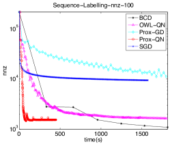
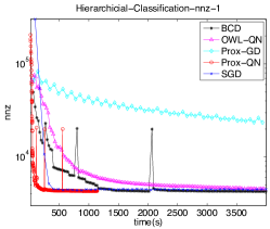
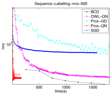
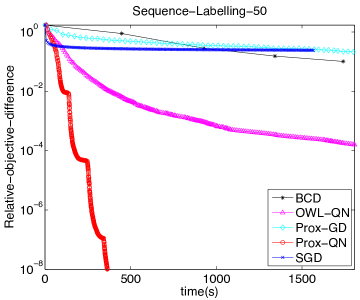
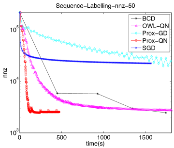
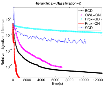
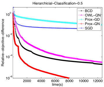
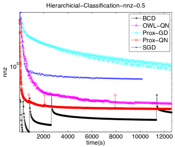
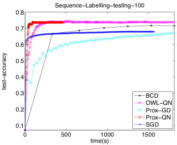
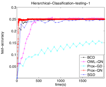
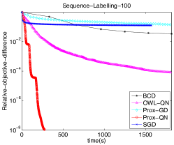
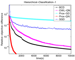
We evaluate the performance of Prox-QN method on two problems, sequence labeling and hierarchical classification. In particular, we plot the relative objective difference (f(𝒘t)f(𝒘))/f(𝒘)𝑓subscript𝒘𝑡𝑓superscript𝒘𝑓superscript𝒘(f(\boldsymbol{w}_{t})-f(\boldsymbol{w}^{*}))/f(\boldsymbol{w}^{*}) and the number of non-zero parameters (on a log scale) against time in seconds. More experiment results, for example, the testing accuracy and the performance for different λ𝜆\lambda’s, are in Appendix E. All the experiments are executed on 2.8GHz Intel Xeon E5-2680 v2 Ivy Bridge processor with 1/4TB memory and Linux OS.

6.1 Sequence Labeling

In sequence labeling problems, each instance (𝒙,𝒚)={(𝒙t,yt)}t=1,2,T𝒙𝒚subscriptsubscript𝒙𝑡subscript𝑦𝑡𝑡12𝑇(\boldsymbol{x},\boldsymbol{y})=\left\{(\boldsymbol{x}_{t},y_{t})\right\}_{t=1,2...,T} is a sequence of T𝑇T pairs of observations and the corresponding labels. Here we consider the optical character recognition (OCR) problem, which aims to recognize the handwriting words. The dataset 222http://www.seas.upenn.edu/ taskar/ocr/ was preprocessed by Taskar et al. [19] and was originally collected by Kassel [20], and contains 6877 words (instances). We randomly divide the dataset into two part: training part with 6216 words and testing part with 661 words. The character label set Y𝑌Y consists of 26 English letters and the observations are characters which are represented by images of 16 by 8 binary pixels as shown in Figure 1(a). We use degree 2 pixels as the raw features, which means all pixel pairs are considered. Therefore, the number of raw features is J=128×127/2+128+1𝐽12812721281J=128\times 127/2+128+1, including a bias. For degree 2 features, xtj=1subscript𝑥𝑡𝑗1x_{tj}=1 only when both pixels are 111 and otherwise xtj=0subscript𝑥𝑡𝑗0x_{tj}=0, where xtjsubscript𝑥𝑡𝑗x_{tj} is the j-th raw feature of 𝒙isubscript𝒙𝑖\boldsymbol{x}_{i}. For the feature functions, we use unigram feature functions 𝟏(yt=y,xtj=1)1formulae-sequencesubscript𝑦𝑡𝑦subscript𝑥𝑡𝑗1\boldsymbol{1}(y_{t}=y,x_{tj}=1) and bigram feature functions 𝟏(yt=y,yt+1=y)1formulae-sequencesubscript𝑦𝑡𝑦subscript𝑦𝑡1superscript𝑦\boldsymbol{1}(y_{t}=y,y_{t+1}=y^{\prime}) with their associated weights, Θy,jsubscriptΘ𝑦𝑗\Theta_{y,j} and Λy,ysubscriptΛ𝑦superscript𝑦\Lambda_{y,y^{\prime}}, respectively. So 𝒘={Θ,Λ}𝒘ΘΛ\boldsymbol{w}=\{\Theta,\Lambda\} for Θ|Y|×JΘsuperscript𝑌𝐽\Theta\in{\mathbb{R}}^{|Y|\times J} and Λ|Y|×|Y|Λsuperscript𝑌𝑌\Lambda\in{\mathbb{R}}^{|Y|\times|Y|} and the total number of parameters, d=|Y|2+|Y|×J=215,358formulae-sequence𝑑superscript𝑌2𝑌𝐽215358d={|Y|}^{2}+|Y|\times J=215,358. Using the above feature functions, the potential function can be specified as, P~𝒘(𝒚,𝒙)=exp{Λ,t=1T(𝒆yt𝒙tT)+Θ,t=1T1(𝒆yt𝒆yt+1T)}subscript~𝑃𝒘𝒚𝒙Λsuperscriptsubscript𝑡1𝑇subscript𝒆subscript𝑦𝑡subscriptsuperscript𝒙𝑇𝑡Θsuperscriptsubscript𝑡1𝑇1subscript𝒆subscript𝑦𝑡subscriptsuperscript𝒆𝑇subscript𝑦𝑡1\tilde{P}_{\boldsymbol{w}}(\boldsymbol{y},\boldsymbol{x})=\exp\left\{\langle\Lambda,\sum_{t=1}^{T}(\boldsymbol{e}_{y_{t}}\boldsymbol{x}^{T}_{t})\rangle+\langle\Theta,\sum_{t=1}^{T-1}(\boldsymbol{e}_{y_{t}}\boldsymbol{e}^{T}_{y_{t+1}})\rangle\right\},where ,\langle\cdot,\cdot\rangle is the sum of element-wise product and 𝒆y|Y|subscript𝒆𝑦superscript𝑌\boldsymbol{e}_{y}\in{\mathbb{R}}^{|Y|} is an unit vector with 1 at y-th entry and 0 at other entries. The gradient and the inference oracle are given in Appendix D.1.

In our experiment, λ𝜆\lambda is set as 100100100, which leads to a relative high testing accuracy and an optimal solution with a relative small number of non-zero parameters (see Appendix E.2). The learning rate η0subscript𝜂0\eta_{0} for SGD is tuned to be 2×1042superscript1042\times 10^{-4} for best performance. In BCD, the unigram parameters are grouped into J𝐽J blocks according to the 𝒙𝒙\boldsymbol{x} features while the bigram parameters are grouped into one block. Our proximal quasi-Newton method can be seen to be much faster than the other methods.
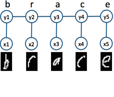
Refer to caption
(a) Graphical model of OCR
Refer to caption
(b) Relative Objective Difference
Refer to caption
(c) Non-zero Parameters
Figure 1: Sequence Labeling Problem

6.2 Hierarchical Classification

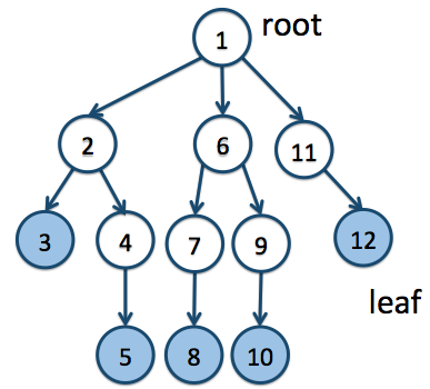
In hierarchical classification problems, we have a label taxonomy, where the classes are grouped into a tree as shown in Figure 2(a). Here y𝒴𝑦𝒴y\in\mathcal{Y} is one of the leaf nodes. If we have totally K𝐾K classes (number of nodes) and J𝐽J raw features, then the number of parameters is d=K×J𝑑𝐾𝐽d=K\times J. Let WK×J𝑊superscript𝐾𝐽W\in{\mathbb{R}}^{K\times J} denote the weights. The feature function corresponding to Wk,jsubscript𝑊𝑘𝑗W_{k,j} is fk,j(y,𝒙)=𝟏[kPath(y)]xjsubscript𝑓𝑘𝑗𝑦𝒙1delimited-[]𝑘Path𝑦subscript𝑥𝑗f_{k,j}(y,\boldsymbol{x})=\boldsymbol{1}[k\in\text{Path}(y)]x_{j}, where kPath(y)𝑘Path(y)k\in\text{Path(y)} means class k𝑘k is an ancestor of y𝑦y or y𝑦y itself. The potential function is P~W(y,𝒙)=exp{kPath(y)𝒘kT𝒙}subscript~𝑃𝑊𝑦𝒙subscript𝑘Path𝑦subscriptsuperscript𝒘𝑇𝑘𝒙\tilde{P}_{W}(y,\boldsymbol{x})=\exp\left\{\sum_{k\in\text{Path}(y)}\boldsymbol{w}^{T}_{k}\boldsymbol{x}\right\} where 𝒘kTsubscriptsuperscript𝒘𝑇𝑘\boldsymbol{w}^{T}_{k} is the weight vector of k-th class, i.e. the k-th row of W𝑊W. The gradient and the inference oracle are given in Appendix D.2.

The dataset comes from Task1 of the dry-run dataset of LSHTC1333http://lshtc.iit.demokritos.gr/node/1. It has 4,463 samples, each with J𝐽J=51,033 raw features. The hierarchical tree has 2,388 classes which includes 1,139 leaf labels. Thus, the number of the parameters d=𝑑absentd=121,866,804. The feature values are scaled by svm-scale program in the LIBSVM package. We set λ=1𝜆1\lambda=1 to achieve a relative high testing accuracy and high sparsity of the optimal solution. The SGD initial learning rate is tuned to be η0=10subscript𝜂010\eta_{0}=10 for best performance. In BCD, parameters are grouped into J𝐽J blocks according to the raw features.
Refer to caption
(a) Label Taxonomy
Refer to caption
(b) Relative Objective Difference
Refer to caption
(c) Non-zero Parameters
Figure 2: Hierarchical Classification Problem

As both Figure 1(b),1(c) and Figure 2(b),2(c) show, Prox-QN achieves much faster convergence and moreover obtains a sparse model in much less time.

Acknowledgement

This research was supported by NSF grants CCF-1320746 and CCF-1117055. P.R. acknowledges the support of ARO via W911NF-12-1-0390 and NSF via IIS-1149803, IIS-1320894, IIS-1447574, and DMS-1264033. K.Z. acknowledges the support of the National Initiative for Modeling and Simulation fellowship

References

  • [1] I. E.H. Yen, C.-J. Hsieh, P. Ravikumar, and I. S. Dhillon. Constant Nullspace Strong Convexity and Fast Convergence of Proximal Methods under High-Dimensional Settings. In NIPS 2014.
  • [2] X. Tang and K. Scheinberg. Efficiently Using Second Order Information in Large l1 Regularization Problems. arXiv:1303.6935, 2013.
  • [3] J. D. Lee, Y. Sun, and M. A. Saunders. Proximal newton-type methods for minimizing composite functions. In NIPS 2012.
  • [4] M. Schmidt, E. Van Den Berg, M.P. Friedlander, and K. Murphy. Optimizing costly functions with simple constraints: A limited-memory projected Quasi-Newton algorithm. In Int. Conf. Artif. Intell. Stat., 2009.
  • [5] C.-J. Hsieh, M. A. Sustik, I. S. Dhillon, and P. Ravikumar. Sparse inverse covariance estimation using quadratic approximation. In NIPS 2011.
  • [6] S. Boyd and L. Vandenberghe. Convex Optimization, Cambridge Univ. Press, Cambridge, U.K., 2003.
  • [7] P.-W. Wang and C.-J. Lin. Iteration Complexity of Feasible Descent Methods for Convex Optimization. Technical report, Department of Computer Science, National Taiwan University, Taipei, Taiwan, 2013.
  • [8] G.-X. Yuan, K.-W. Chang, C.-J. Hsieh, and C.-J. Lin. A comparison of optimization methods and software for large-scale l1-regularized linear classification. Journal of Machine Learning Research (JMLR), 11:3183-3234, 2010.
  • [9] A. Agarwal, S. Negahban, and M. Wainwright. Fast Global Convergence Rates of Gradient Methods for High-Dimensional Statistical Recovery. In NIPS 2010.
  • [10] K. Hou, Z. Zhou, A. M.-S. So, and Z.-Q. Luo. On the linear convergence of the proximal gradient method for trace norm regularization. In NIPS 2014.
  • [11] L. Xiao and T. Zhang. A proximal-gradient homotopy method for the l1-regularized least-squares problem. In ICML 2012.
  • [12] P. Tseng and S. Yun. A coordinate gradient descent method for nonsmooth separable minimization, Math. Prog. B. 117, 2009.
  • [13] G.-X. Yuan, C.-H. Ho, and C.-J. Lin. An improved GLMNET for l1-regularized logistic regression, JMLR, 13:1999 -2030, 2012.
  • [14] R.-E. Fan, K.-W. Chang, C.-J. Hsieh, X.-R. Wang, and C.-J. Lin. LIBLINEAR: A library for large linear classification, JMLR, 9:1871-1874, 2008.
  • [15] A. J Hoffman. On approximate solutions of systems of linear inequalities. Journal of Research of the National Bureau of Standards, 1952.
  • [16] N. Sokolovska, T. Lavergne, O. Cappe, and F. Yvon. Efficient Learning of Sparse Conditional Random Fields for Supervised Sequence Labelling. arXiv:0909.1308, 2009.
  • [17] Y. Tsuboi, Y. Unno, H. Kashima, and N. Okazaki. Fast Newton-CG Method for Batch Learning of Conditional Random Fields, Proceedings of the Twenty-Fifth AAAI Conference on Artificial Intelligence, 2011.
  • [18] J. Nocedal and S. J. Wright. Numerical Optimization. Springer Series in Operations Research. Springer, New York, NY, USA, 2nd edition, 2006.
  • [19] B. Taskar, C. Guestrin, and D. Koller. Max-margin markov networks. In NIPS 2003.
  • [20] R. Kassel. A Comparison of Approaches to On-line Handwritten Character Recognition. PhD thesis, MIT Spoken Language Systems Group, 1995.
  • [21] Y. Tsuruoka, J. Tsujii, and S. Ananiadou. Stochastic gradient descent training for l1- regularized log-linear models with cumulative penalty. In Proceedings of the Joint Conference of the 47th Annual Meeting of the ACL and the 4th International Joint Conference on Natural Language Processing of the AFNLP, pages 477-485, Suntec, Singapore, 2009.
  • [22] J. Yu, S.V.N. Vishwanathan, S. Gunter, and N. N. Schraudolph. A Quasi-Newton approach to nonsmooth convex optimization problems in machine learning, JMLR, 11:1-57, 2010.
  • [23] G. Andrew and J. Gao. Scalable training of 1subscript1\ell_{1}-regularized log-linear models. In ICML 2007.
  • [24] J.E. Dennis and J.J. More. A characterization of superlinear convergence and its application to Quasi-Newton methods. Math. Comp., 28(126):549 560, 1974.
  • [25] K. Scheinberg and X. Tang. Practical Inexact Proximal Quasi-Newton Method with Global Complexity Analysis. COR@L Technical Report at Lehigh University. arXiv:1311.6547, 2013
  • [26] J. D. Lee, Y. Sun, and M. A. Saunders. Proximal Newton-type methods for minimizing composite functions. arXiv:1206.1623, 2012
  • [27] M. J. Wainwright and M. I. Jordan. Graphical models, exponential families, and variational inference. Technical Report 649, Dept. Statistics, Univ. California, Berkeley. 2003

APPENDIX

Appendix A Convergence Proof

To exploit the CNSC-𝒯𝒯\mathcal{T} property, we first re-build our problem and algorithm on the reduced space 𝒵={𝒛d^|𝒛=UT𝒘}𝒵conditional-set𝒛superscript^𝑑𝒛superscript𝑈𝑇𝒘\mathcal{Z}=\{\boldsymbol{z}\in{\mathbb{R}}^{\hat{d}}|\boldsymbol{z}=U^{T}\boldsymbol{w}\}, where the strong-convexity property holds. Then we prove the asymptotic super-linear convergence on 𝒵𝒵\mathcal{Z} under the condition that the inner problem is solved exactly and no shrinking strategy is not applied. Finally we prove the objective (1) is bounded by the difference between current iterate and the optimal solution. In Section A.5, we provide the global convergence proof when the shrinking strategy is applied.

A.1 Representing the problem in a reduced and compact space

Properties of CNSC-𝒯𝒯\mathcal{T} condition
For (𝒘)𝒘\ell(\boldsymbol{w}) satisfying CNSC-𝒯𝒯\mathcal{T} condition, we have (𝒘)=(𝐩𝐫𝐨𝐣𝒯(𝒘))𝒘subscript𝐩𝐫𝐨𝐣𝒯𝒘\ell(\boldsymbol{w})=\ell(\mathbf{proj}_{\mathcal{T}}(\boldsymbol{w})). Define 𝒈𝒈\boldsymbol{g} to be the gradient of (𝒘)𝒘\ell(\boldsymbol{w}) and H𝐻H to be the Hessian of (𝒘)𝒘\ell(\boldsymbol{w}). As both 𝒈𝒈\boldsymbol{g} and H𝐻H are in the 𝒯𝒯\mathcal{T} space, we have 𝒈(𝒘)=UUT𝒈(𝐩𝐫𝐨𝐣𝒯(𝒘))=𝒈(𝐩𝐫𝐨𝐣𝒯(𝒘))𝒈𝒘𝑈superscript𝑈𝑇𝒈subscript𝐩𝐫𝐨𝐣𝒯𝒘𝒈subscript𝐩𝐫𝐨𝐣𝒯𝒘\boldsymbol{g}(\boldsymbol{w})=UU^{T}\boldsymbol{g}(\mathbf{proj}_{\mathcal{T}}(\boldsymbol{w}))=\boldsymbol{g}(\mathbf{proj}_{\mathcal{T}}(\boldsymbol{w})) and H(𝒘)=UUTH(𝐩𝐫𝐨𝐣𝒯(𝒘))UUT=H(𝐩𝐫𝐨𝐣𝒯(𝒘))𝐻𝒘𝑈superscript𝑈𝑇𝐻subscript𝐩𝐫𝐨𝐣𝒯𝒘𝑈superscript𝑈𝑇𝐻subscript𝐩𝐫𝐨𝐣𝒯𝒘H(\boldsymbol{w})=UU^{T}H(\mathbf{proj}_{\mathcal{T}}(\boldsymbol{w}))UU^{T}=H(\mathbf{proj}_{\mathcal{T}}(\boldsymbol{w})).

Objective formulation in the reduced space
Define ^(𝒛)=(U𝒛)^𝒛𝑈𝒛\hat{\ell}(\boldsymbol{z})=\ell(U\boldsymbol{z}). Then if 𝒛=UT𝒘𝒛superscript𝑈𝑇𝒘\boldsymbol{z}=U^{T}\boldsymbol{w}, we have ^(𝒛)=(𝒘)^𝒛𝒘\hat{\ell}(\boldsymbol{z})=\ell(\boldsymbol{w}), 𝒈^(𝒛)=UT𝒈(𝒘)^𝒈𝒛superscript𝑈𝑇𝒈𝒘\hat{\boldsymbol{g}}(\boldsymbol{z})=U^{T}\boldsymbol{g}(\boldsymbol{w}) and H^(𝒛)=UTH(𝒘)U^𝐻𝒛superscript𝑈𝑇𝐻𝒘𝑈\hat{H}(\boldsymbol{z})=U^{T}H(\boldsymbol{w})U, where 𝒈^(𝒛)^𝒈𝒛\hat{\boldsymbol{g}}(\boldsymbol{z}) and H^(𝒛)^𝐻𝒛\hat{H}(\boldsymbol{z}) are the gradient and Hessian of ^(𝒛)^𝒛\hat{\ell}(\boldsymbol{z}) respectively. Now H^^𝐻\hat{H} is positive definite with minimal eigenvalue m𝑚m. The objective (1) can be re-formulated in the reduced space by

min𝒛f^(𝒛)=h(𝒛)+^(𝒛),subscript𝒛^𝑓𝒛𝒛^𝒛\min_{\boldsymbol{z}}\hat{f}(\boldsymbol{z})=h(\boldsymbol{z})+\hat{\ell}(\boldsymbol{z}), (8)

where

h(𝒛)=minUT𝒘=𝒛λ𝒘1𝒛subscriptsuperscript𝑈𝑇𝒘𝒛𝜆subscriptnorm𝒘1h(\boldsymbol{z})=\min_{U^{T}\boldsymbol{w}=\boldsymbol{z}}\lambda\|\boldsymbol{w}\|_{1}

We now prove that h(𝒛)𝒛h(\boldsymbol{z}) is a convex function, i.e.,

ch(𝒛1)+(1c)h(𝒛2)h(c𝒛1+(1c)𝒛2)𝑐subscript𝒛11𝑐subscript𝒛2𝑐subscript𝒛11𝑐subscript𝒛2ch(\boldsymbol{z}_{1})+(1-c)h(\boldsymbol{z}_{2})\geq h(c\boldsymbol{z}_{1}+(1-c)\boldsymbol{z}_{2})

for any 0c10𝑐10\leq c\leq 1, 𝒛1subscript𝒛1\boldsymbol{z}_{1} and 𝒛2subscript𝒛2\boldsymbol{z}_{2}.

Proof.

Let

𝒘1=argminUT𝒘=𝒛1λw1 and 𝒘2=argminUT𝒘=𝒛2λw1subscript𝒘1superscript𝑈𝑇𝒘subscript𝒛1argmin𝜆subscriptnorm𝑤1 and subscript𝒘2superscript𝑈𝑇𝒘subscript𝒛2argmin𝜆subscriptnorm𝑤1\boldsymbol{w}_{1}=\underset{U^{T}\boldsymbol{w}=\boldsymbol{z}_{1}}{\text{argmin}}\lambda\|w\|_{1}\text{ and }\boldsymbol{w}_{2}=\underset{U^{T}\boldsymbol{w}=\boldsymbol{z}_{2}}{\text{argmin}}\lambda\|w\|_{1}

Then,

ch(𝒛1)+(1c)h(𝒛2)𝑐subscript𝒛11𝑐subscript𝒛2\displaystyle ch(\boldsymbol{z}_{1})+(1-c)h(\boldsymbol{z}_{2}) =λ(c𝒘11+(1c)𝒘21)absent𝜆𝑐subscriptnormsubscript𝒘111𝑐subscriptnormsubscript𝒘21\displaystyle=\lambda(c\|\boldsymbol{w}_{1}\|_{1}+(1-c)\|\boldsymbol{w}_{2}\|_{1})
λ(c𝒘1+(1c)𝒘21)absent𝜆subscriptnorm𝑐subscript𝒘11𝑐subscript𝒘21\displaystyle\geq\lambda(\|c\boldsymbol{w}_{1}+(1-c)\boldsymbol{w}_{2}\|_{1})
h(UT(c𝒘1+(1c)𝒘2))absentsuperscript𝑈𝑇𝑐subscript𝒘11𝑐subscript𝒘2\displaystyle\geq h(U^{T}(c\boldsymbol{w}_{1}+(1-c)\boldsymbol{w}_{2}))
=h(c𝒛1+(1c)𝒛2)absent𝑐subscript𝒛11𝑐subscript𝒛2\displaystyle=h(c\boldsymbol{z}_{1}+(1-c)\boldsymbol{z}_{2})

The optimal solution 𝒛superscript𝒛\boldsymbol{z}^{*} of (8) has the following relationship with the optimal solution 𝒘superscript𝒘\boldsymbol{w}^{*} of (1) ,

𝒘=argminUT𝒘=𝒛 λ𝒘1 and 𝒛=UT𝒘superscript𝒘superscript𝑈𝑇𝒘superscript𝒛argmin 𝜆subscriptnorm𝒘1 and superscript𝒛superscript𝑈𝑇superscript𝒘\boldsymbol{w}^{*}=\underset{U^{T}\boldsymbol{w}=\boldsymbol{z}^{*}}{\text{argmin}}\textit{ }\lambda\|\boldsymbol{w}\|_{1}\text{ and }\boldsymbol{z}^{*}=U^{T}\boldsymbol{w}^{*} (9)

Lipschitz continuity in the reduced space
Throughout the paper, we assume the Hessian of (𝒘)𝒘\ell(\boldsymbol{w}) has Lipschitz continuity with constant LHsubscript𝐿𝐻L_{H}. According to the Lipschitz continuity,

H(𝒘2)(𝒘1𝒘2)(𝒈(𝒘1)𝒈(𝒘2))LH2𝒘1𝒘22norm𝐻subscript𝒘2subscript𝒘1subscript𝒘2𝒈subscript𝒘1𝒈subscript𝒘2subscript𝐿𝐻2superscriptnormsubscript𝒘1subscript𝒘22\|H(\boldsymbol{w}_{2})(\boldsymbol{w}_{1}-\boldsymbol{w}_{2})-(\boldsymbol{g}(\boldsymbol{w}_{1})-\boldsymbol{g}(\boldsymbol{w}_{2}))\|\leq\frac{L_{H}}{2}\|\boldsymbol{w}_{1}-\boldsymbol{w}_{2}\|^{2}

In the corresponding reduced space, the Lipschitz continuity also holds with the same constant .

H^(𝒛2)(𝒛1𝒛2)(𝒈^(𝒛1)𝒈^(𝒛2))LH2𝒛1𝒛22norm^𝐻subscript𝒛2subscript𝒛1subscript𝒛2^𝒈subscript𝒛1^𝒈subscript𝒛2subscript𝐿𝐻2superscriptnormsubscript𝒛1subscript𝒛22\|\hat{H}(\boldsymbol{z}_{2})(\boldsymbol{z}_{1}-\boldsymbol{z}_{2})-(\hat{\boldsymbol{g}}(\boldsymbol{z}_{1})-\hat{\boldsymbol{g}}(\boldsymbol{z}_{2}))\|\leq\frac{L_{H}}{2}\|\boldsymbol{z}_{1}-\boldsymbol{z}_{2}\|^{2} (10)

BFGS update formula in the reduced space
If B0subscript𝐵0B_{0} is in the 𝒯𝒯\mathcal{T} space, Btsubscript𝐵𝑡B_{t} is also in the 𝒯𝒯\mathcal{T} space. This can be shown by re-formulating the BFGS update and mathematical induction,

Bt=UB^t1UTUB^t1UTst1st1TUB^t1UTst1TUB^t1UTst1+UUTyt1yt1TUUTyt1TUUTst1subscript𝐵𝑡𝑈subscript^𝐵𝑡1superscript𝑈𝑇𝑈subscript^𝐵𝑡1superscript𝑈𝑇subscript𝑠𝑡1subscriptsuperscript𝑠𝑇𝑡1𝑈subscript^𝐵𝑡1superscript𝑈𝑇superscriptsubscript𝑠𝑡1𝑇𝑈subscript^𝐵𝑡1superscript𝑈𝑇subscript𝑠𝑡1𝑈superscript𝑈𝑇subscript𝑦𝑡1subscriptsuperscript𝑦𝑇𝑡1𝑈superscript𝑈𝑇superscriptsubscript𝑦𝑡1𝑇𝑈superscript𝑈𝑇subscript𝑠𝑡1B_{t}=U\hat{B}_{t-1}U^{T}-\frac{U\hat{B}_{t-1}U^{T}s_{t-1}s^{T}_{t-1}U\hat{B}_{t-1}U^{T}}{s_{t-1}^{T}U\hat{B}_{t-1}U^{T}s_{t-1}}+\frac{UU^{T}y_{t-1}y^{T}_{t-1}UU^{T}}{y_{t-1}^{T}UU^{T}s_{t-1}} (11)

Thus

B^t=B^t1B^t1s^t1s^t1TB^t1s^t1TB^t1s^t1+y^t1y^t1Ty^t1Ts^t1subscript^𝐵𝑡subscript^𝐵𝑡1subscript^𝐵𝑡1subscript^𝑠𝑡1subscriptsuperscript^𝑠𝑇𝑡1subscript^𝐵𝑡1superscriptsubscript^𝑠𝑡1𝑇subscript^𝐵𝑡1subscript^𝑠𝑡1subscript^𝑦𝑡1subscriptsuperscript^𝑦𝑇𝑡1superscriptsubscript^𝑦𝑡1𝑇subscript^𝑠𝑡1\hat{B}_{t}=\hat{B}_{t-1}-\frac{\hat{B}_{t-1}\hat{s}_{t-1}\hat{s}^{T}_{t-1}\hat{B}_{t-1}}{\hat{s}_{t-1}^{T}\hat{B}_{t-1}\hat{s}_{t-1}}+\frac{\hat{y}_{t-1}\hat{y}^{T}_{t-1}}{\hat{y}_{t-1}^{T}\hat{s}_{t-1}} (12)

where s^=UTs^𝑠superscript𝑈𝑇𝑠\hat{s}=U^{T}s, y^=UTy^𝑦superscript𝑈𝑇𝑦\hat{y}=U^{T}y and UB^tUT=Bt𝑈subscript^𝐵𝑡superscript𝑈𝑇subscript𝐵𝑡U\hat{B}_{t}U^{T}=B_{t}. It can be proved that B^tsubscript^𝐵𝑡\hat{B}_{t} generated in (12) is positive definite provided y^Ts^>0superscript^𝑦𝑇^𝑠0\hat{y}^{T}\hat{s}>0 [18]. If we additionally assume m𝒛2𝒛TB^t𝒛M𝒛2𝑚superscriptnorm𝒛2superscript𝒛𝑇subscript^𝐵𝑡𝒛𝑀superscriptnorm𝒛2m\|\boldsymbol{z}\|^{2}\leq\boldsymbol{z}^{T}\hat{B}_{t}\boldsymbol{z}\leq M\|\boldsymbol{z}\|^{2} for any 𝒛d^𝒛superscript^𝑑\boldsymbol{z}\in{\mathbb{R}}^{\hat{d}}, then Btsubscript𝐵𝑡B_{t} satisfies the CNSC-𝒯𝒯\mathcal{T} condition.

Iterate in the reduced space
The potential new iterate 𝒘+superscript𝒘\boldsymbol{w}^{+} is

𝒘+=argmin𝒗 λ𝒗1+12(𝒗𝒘t)TBt(𝒗𝒘t)+𝒈tT(𝒗𝒘t)superscript𝒘𝒗argmin 𝜆subscriptnorm𝒗112superscript𝒗subscript𝒘𝑡𝑇subscript𝐵𝑡𝒗subscript𝒘𝑡superscriptsubscript𝒈𝑡𝑇𝒗subscript𝒘𝑡\boldsymbol{w}^{+}=\underset{\boldsymbol{v}}{\text{argmin}}\textit{ }\lambda\|\boldsymbol{v}\|_{1}+\frac{1}{2}(\boldsymbol{v}-\boldsymbol{w}_{t})^{T}B_{t}(\boldsymbol{v}-\boldsymbol{w}_{t})+\boldsymbol{g}_{t}^{T}(\boldsymbol{v}-\boldsymbol{w}_{t}) (13)

In the reduced space, the potential new iterate (13) can be represented by,

𝒛+=argmin𝒙 h(𝒙)+12(𝒙𝒛t)TB^t(𝒙𝒛t)+𝒈^tT(𝒙𝒛t)superscript𝒛𝒙argmin 𝒙12superscript𝒙subscript𝒛𝑡𝑇subscript^𝐵𝑡𝒙subscript𝒛𝑡superscriptsubscript^𝒈𝑡𝑇𝒙subscript𝒛𝑡\boldsymbol{z}^{+}=\underset{\boldsymbol{x}}{\text{argmin}}\textit{ }h(\boldsymbol{x})+\frac{1}{2}(\boldsymbol{x}-\boldsymbol{z}_{t})^{T}\hat{B}_{t}(\boldsymbol{x}-\boldsymbol{z}_{t})+\hat{\boldsymbol{g}}_{t}^{T}(\boldsymbol{x}-\boldsymbol{z}_{t}) (14)

𝒛+superscript𝒛\boldsymbol{z}^{+} and 𝒘+superscript𝒘\boldsymbol{w}^{+} also satisfy Equation (9), i.e.

𝒘+=argminUT𝒘=𝒛+ 𝒘1superscript𝒘superscript𝑈𝑇𝒘superscript𝒛argmin subscriptnorm𝒘1\boldsymbol{w}^{+}=\underset{U^{T}\boldsymbol{w}=\boldsymbol{z}^{+}}{\text{argmin}}\textit{ }\|\boldsymbol{w}\|_{1} (15)

In this paper, we consider the convergence phase when 𝒛tsubscript𝒛𝑡\boldsymbol{z}_{t} is close enough to the optimum such that the unit step size is always chosen, i.e. 𝒛t+1=𝒛+subscript𝒛𝑡1superscript𝒛\boldsymbol{z}_{t+1}=\boldsymbol{z}^{+} [26].

A.2 Global linear Convergence

Lemma 1 (Global linear Convergence).

For ^(𝐳)^𝐳\nabla\hat{\ell}(\boldsymbol{z}) satisfying Lipschitz-continuity with a constant Lgsubscript𝐿𝑔L_{g} and Btsubscript𝐵𝑡B_{t} satisfying CNSC-𝒯𝒯\mathcal{T}, the sequence {𝐳t}t=1superscriptsubscriptsubscript𝐳𝑡𝑡1\{\boldsymbol{z}_{t}\}_{t=1}^{\infty} produced by Prox-QN method converges at least R-linearly.

Proof.

This theorem follows Theorem 2 in [12], where the coordinate block Jksubscript𝐽𝑘J_{k} is chosen to be the whole coordinate set. Assumption 2(a) in [12] is satisfied because of Theorem 4 C4 in [12] by assuming ^(𝒛)^𝒛\nabla\hat{\ell}(\boldsymbol{z}) is Lipschitz-continuous. Other conditions of Theorem 2 in [12] can be easily justified. ∎

A.3 Quadratic Convergence of Proximal Newton Method and Dennis-More Criterion

Lemma 2 (Quadratic Convergence of Prox-Newton (Theorem 3 in [1])).

For (𝐰)𝐰\ell(\boldsymbol{w}) satisfying CNSC-𝒯𝒯\mathcal{T} with Lipschitz-continuous second derivative H(𝐰)=2(𝐰)𝐻𝐰superscript2𝐰H(\boldsymbol{w})=\nabla^{2}\ell(\boldsymbol{w}), the sequence {𝐰t}subscript𝐰𝑡\{\boldsymbol{w}_{t}\} produced by proximal Newton Method in the quadratic convergence phase has

𝒛t+1𝒛LH2m𝒛t𝒛2,normsubscript𝒛𝑡1superscript𝒛subscript𝐿𝐻2𝑚superscriptnormsubscript𝒛𝑡superscript𝒛2\|\boldsymbol{z}_{t+1}-\boldsymbol{z}^{*}\|\leq\frac{L_{H}}{2m}\|\boldsymbol{z}_{t}-\boldsymbol{z}^{*}\|^{2},

where 𝐳=UT𝐰superscript𝐳superscript𝑈𝑇superscript𝐰\boldsymbol{z}^{*}=U^{T}\boldsymbol{w}^{*}, 𝐳t=UT𝐰tsubscript𝐳𝑡superscript𝑈𝑇subscript𝐰𝑡\boldsymbol{z}_{t}=U^{T}\boldsymbol{w}_{t}, 𝐰superscript𝐰\boldsymbol{w}^{*} is the optimal solution and LHsubscript𝐿𝐻L_{H} is the Lipschitz constant for H(𝐰)𝐻𝐰H(\boldsymbol{w}).

Lemma 3.

If B0=UB^0UTsubscript𝐵0𝑈subscript^𝐵0superscript𝑈𝑇B_{0}=U\hat{B}_{0}U^{T} satisfies CNSC-𝒯𝒯\mathcal{T} condition, then B^tsubscript^𝐵𝑡\hat{B}_{t} generated by (12) satisfies the Dennis-More criterion [24], namely,

limt(B^tH^)(𝒛t+1𝒛t)𝒛t+1𝒛t=0,subscript𝑡normsubscript^𝐵𝑡superscript^𝐻subscript𝒛𝑡1subscript𝒛𝑡normsubscript𝒛𝑡1subscript𝒛𝑡0\lim_{t\rightarrow\infty}\frac{\|(\hat{B}_{t}-\hat{H}^{*})(\boldsymbol{z}_{t+1}-\boldsymbol{z}_{t})\|}{\|\boldsymbol{z}_{t+1}-\boldsymbol{z}_{t}\|}=0,

where H^=2^(𝐳)superscript^𝐻superscript2^superscript𝐳\hat{H}^{*}=\nabla^{2}\hat{\ell}(\boldsymbol{z}^{*}) and 𝐳superscript𝐳\boldsymbol{z}^{*} is the optimal solution of (8).

Proof.

We want to show that this proof can follow the proof of Theorem 6.6 in [18]. We will verify that the conditions of Theorem 6.6 in [18] are satisfied here. First, the Lipschitz continuity of H^(𝒛)^𝐻𝒛\hat{H}(\boldsymbol{z}) is implied by Lipschitz continuity of H(𝒘)𝐻𝒘H(\boldsymbol{w}) :

(H^(𝒛1)H^(𝒛2))norm^𝐻subscript𝒛1^𝐻subscript𝒛2\displaystyle\|(\hat{H}(\boldsymbol{z}_{1})-\hat{H}(\boldsymbol{z}_{2}))\| =UT(H(𝒘1)H(𝒘2))Uabsentnormsuperscript𝑈𝑇𝐻subscript𝒘1𝐻subscript𝒘2𝑈\displaystyle=\|U^{T}(H(\boldsymbol{w}_{1})-H(\boldsymbol{w}_{2}))U\|
H(𝒘1)H(𝒘2)absentnorm𝐻subscript𝒘1𝐻subscript𝒘2\displaystyle\leq\|H(\boldsymbol{w}_{1})-H(\boldsymbol{w}_{2})\|
=H(U𝒛1)H(U𝒛2)absentnorm𝐻𝑈subscript𝒛1𝐻𝑈subscript𝒛2\displaystyle=\|H(U\boldsymbol{z}_{1})-H(U\boldsymbol{z}_{2})\|
LH𝒛1𝒛2absentsubscript𝐿𝐻normsubscript𝒛1subscript𝒛2\displaystyle\leq L_{H}\|\boldsymbol{z}_{1}-\boldsymbol{z}_{2}\|

where the last inequality is from the Lipschitz continuity of H(𝒘)𝐻𝒘H(\boldsymbol{w}). The second condition, t=0𝒛t𝒛<superscriptsubscript𝑡0normsubscript𝒛𝑡superscript𝒛\sum_{t=0}^{\infty}\|\boldsymbol{z}_{t}-\boldsymbol{z}^{*}\|<\infty, is implied by the global linear convergence(Lemma 1). ∎

A.4 Asymptotic Superlinear Convergence

Proof of Theorem 1

Proof.

If Btsubscript𝐵𝑡B_{t} satisfies CNSC-𝒯𝒯\mathcal{T} condition, then B^tsubscript^𝐵𝑡\hat{B}_{t} satisfies m𝒛2𝒛TB^t𝒛M𝒛2𝑚superscriptnorm𝒛2superscript𝒛𝑇subscript^𝐵𝑡𝒛𝑀superscriptnorm𝒛2m\|\boldsymbol{z}\|^{2}\leq\boldsymbol{z}^{T}\hat{B}_{t}\boldsymbol{z}\leq M\|\boldsymbol{z}\|^{2} for any 𝒛d^𝒛superscript^𝑑\boldsymbol{z}\in{\mathbb{R}}^{\hat{d}}. The Lipschitz-continuous H𝐻H implies Lipschitz-continuity of H^^𝐻\hat{H}. Therefore by applying the Prox-QN method in the reduced space, this theorem follows Theorem 3.7 in [26], Lemma 3 and Lemma 2. ∎

Proof of Theorem 2

Proof.

We prove this theorem by showing |(𝒘t)(𝒘)|L𝒛t𝒛subscript𝒘𝑡superscript𝒘subscript𝐿normsubscript𝒛𝑡superscript𝒛|\ell(\boldsymbol{w}_{t})-\ell(\boldsymbol{w}^{*})|\leq L_{\ell}\|\boldsymbol{z}_{t}-\boldsymbol{z}^{*}\| and 𝒘t1𝒘1d𝒛t𝒛subscriptnormsubscript𝒘𝑡1subscriptnormsuperscript𝒘1𝑑normsubscript𝒛𝑡superscript𝒛\|\boldsymbol{w}_{t}\|_{1}-\|\boldsymbol{w}^{*}\|_{1}\leq\sqrt{d}\|\boldsymbol{z}_{t}-\boldsymbol{z}^{*}\|. The first part is given by,

|(𝒘t)(𝒘)|=|(UUT𝒘t)(UUT𝒘)|LUUT(𝒘t𝒘)=L𝒛t𝒛subscript𝒘𝑡superscript𝒘𝑈superscript𝑈𝑇subscript𝒘𝑡𝑈superscript𝑈𝑇superscript𝒘subscript𝐿norm𝑈superscript𝑈𝑇subscript𝒘𝑡superscript𝒘subscript𝐿normsubscript𝒛𝑡superscript𝒛|\ell(\boldsymbol{w}_{t})-\ell(\boldsymbol{w}^{*})|=|\ell(UU^{T}\boldsymbol{w}_{t})-\ell(UU^{T}\boldsymbol{w}^{*})|\leq L_{\ell}\|UU^{T}(\boldsymbol{w}_{t}-\boldsymbol{w}^{*})\|=L_{\ell}\|\boldsymbol{z}_{t}-\boldsymbol{z}^{*}\|

where the inequality comes from the Lipschitz-continuity of (𝒘)𝒘\ell(\boldsymbol{w}). In the super-linear convergence phase, the unit step size is chosen, so each iterate satisfies (15). We have 𝒘t1UUT𝒘t+(IUUT)𝒘1subscriptnormsubscript𝒘𝑡1subscriptnorm𝑈superscript𝑈𝑇subscript𝒘𝑡𝐼𝑈superscript𝑈𝑇superscript𝒘1\|\boldsymbol{w}_{t}\|_{1}\leq\|UU^{T}\boldsymbol{w}_{t}+(I-UU^{T})\boldsymbol{w}^{*}\|_{1}. Moreover, due to the Lipschitz-continuity of 1subscript1\ell_{1} norm, which is 𝒘1𝒗1d𝒘𝒗subscriptnorm𝒘1subscriptnorm𝒗1𝑑norm𝒘𝒗\|\boldsymbol{w}\|_{1}-\|\boldsymbol{v}\|_{1}\leq\sqrt{d}\|\boldsymbol{w}-\boldsymbol{v}\|, we have,

UUT𝒘t+(IUUT)𝒘1subscriptnorm𝑈superscript𝑈𝑇subscript𝒘𝑡𝐼𝑈superscript𝑈𝑇superscript𝒘1\displaystyle\|UU^{T}\boldsymbol{w}_{t}+(I-UU^{T})\boldsymbol{w}^{*}\|_{1} 𝒘1+dUUT𝒘tUUT𝒘absentsubscriptnormsuperscript𝒘1𝑑norm𝑈superscript𝑈𝑇subscript𝒘𝑡𝑈superscript𝑈𝑇superscript𝒘\displaystyle\leq\|\boldsymbol{w}^{*}\|_{1}+\sqrt{d}\|UU^{T}\boldsymbol{w}_{t}-UU^{T}\boldsymbol{w}^{*}\|
𝒘1+d𝒛t𝒛absentsubscriptnormsuperscript𝒘1𝑑normsubscript𝒛𝑡superscript𝒛\displaystyle\leq\|\boldsymbol{w}^{*}\|_{1}+\sqrt{d}\|\boldsymbol{z}_{t}-\boldsymbol{z}^{*}\|

A.5 Global Convergence with Shrinking

In Theorem 1, we assume shrinking strategy is not employed and the inner problem is solved exactly. In this subsection, we show that by only assuming the inner problem is solved exactly, Prox-QN method with shrinking will still globally converge to the optimum under the CNSC-𝒯𝒯\mathcal{T} condition. We first prove that with sufficient small step size, the Armijo rule will be satisfied.

Lemma 4.

If the step size,

αmin{1,mL1(1σ)}𝛼1𝑚subscript𝐿11𝜎\alpha\leq\min{\{1,\frac{m}{L_{1}}(1-\sigma)\}}

then the Armijo rule is satisfied, i.e.,

f(𝒘+α𝒅)f(𝒘)+ασ(λ𝒘+𝒅1λ𝒘1+𝒈T𝒅)𝑓𝒘𝛼𝒅𝑓𝒘𝛼𝜎𝜆subscriptnorm𝒘𝒅1𝜆subscriptnorm𝒘1superscript𝒈𝑇𝒅f(\boldsymbol{w}+\alpha\boldsymbol{d})\leq f(\boldsymbol{w})+\alpha\sigma(\lambda\|\boldsymbol{w}+\boldsymbol{d}\|_{1}-\lambda\|\boldsymbol{w}\|_{1}+\boldsymbol{g}^{T}\boldsymbol{d})

where L1subscript𝐿1L_{1} is the Lipschitz-continuity constant.

Proof.

Let 𝒘+=𝒘+α𝒅superscript𝒘𝒘𝛼𝒅\boldsymbol{w}^{+}=\boldsymbol{w}+\alpha\boldsymbol{d},

f(𝒘+)f(𝒘)𝑓superscript𝒘𝑓𝒘\displaystyle f(\boldsymbol{w}^{+})-f(\boldsymbol{w}) =(𝒘+)(𝒘)+λ(𝒘+1𝒘1)absentsuperscript𝒘𝒘𝜆subscriptnormsuperscript𝒘1subscriptnorm𝒘1\displaystyle=\ell(\boldsymbol{w}^{+})-\ell(\boldsymbol{w})+\lambda(\|\boldsymbol{w}^{+}\|_{1}-\|\boldsymbol{w}\|_{1})
01(𝒘+sα𝒅)(α𝒅)𝑑s+αλ𝒘+𝒅1+(1α)λ𝒘1λ𝒘1absentsuperscriptsubscript01𝒘𝑠𝛼𝒅𝛼𝒅differential-d𝑠𝛼𝜆subscriptnorm𝒘𝒅11𝛼𝜆subscriptnorm𝒘1𝜆subscriptnorm𝒘1\displaystyle\leq\int_{0}^{1}\nabla\ell(\boldsymbol{w}+s\alpha\boldsymbol{d})(\alpha\boldsymbol{d})ds+\alpha\lambda\|\boldsymbol{w}+\boldsymbol{d}\|_{1}+(1-\alpha)\lambda\|\boldsymbol{w}\|_{1}-\lambda\|\boldsymbol{w}\|_{1}
=α((𝒘)T𝒅+λ𝒘+𝒅1λ𝒘1)+α01𝒅T((𝒘+sα𝒅)(𝒘))𝑑sabsent𝛼superscript𝒘𝑇𝒅𝜆subscriptnorm𝒘𝒅1𝜆subscriptnorm𝒘1𝛼superscriptsubscript01superscript𝒅𝑇𝒘𝑠𝛼𝒅𝒘differential-d𝑠\displaystyle=\alpha(\nabla\ell(\boldsymbol{w})^{T}\boldsymbol{d}+\lambda\|\boldsymbol{w}+\boldsymbol{d}\|_{1}-\lambda\|\boldsymbol{w}\|_{1})+\alpha\int_{0}^{1}\boldsymbol{d}^{T}(\nabla\ell(\boldsymbol{w}+s\alpha\boldsymbol{d})-\nabla\ell(\boldsymbol{w}))ds
α((𝒘)T𝒅+λ𝒘+𝒅1λ𝒘1)+α01UT𝒅(𝒘+sα𝒅)(𝒘)𝑑sabsent𝛼superscript𝒘𝑇𝒅𝜆subscriptnorm𝒘𝒅1𝜆subscriptnorm𝒘1𝛼superscriptsubscript01normsuperscript𝑈𝑇𝒅norm𝒘𝑠𝛼𝒅𝒘differential-d𝑠\displaystyle\leq\alpha(\nabla\ell(\boldsymbol{w})^{T}\boldsymbol{d}+\lambda\|\boldsymbol{w}+\boldsymbol{d}\|_{1}-\lambda\|\boldsymbol{w}\|_{1})+\alpha\int_{0}^{1}\|U^{T}\boldsymbol{d}\|\|\nabla\ell(\boldsymbol{w}+s\alpha\boldsymbol{d})-\nabla\ell(\boldsymbol{w})\|ds

Because

(𝒘+sα𝒅)(𝒘)=(UUT𝒘+sαUUT𝒅)(UUT𝒘)sL1UT𝒅norm𝒘𝑠𝛼𝒅𝒘norm𝑈superscript𝑈𝑇𝒘𝑠𝛼𝑈superscript𝑈𝑇𝒅𝑈superscript𝑈𝑇𝒘𝑠subscript𝐿1normsuperscript𝑈𝑇𝒅\|\nabla\ell(\boldsymbol{w}+s\alpha\boldsymbol{d})-\nabla\ell(\boldsymbol{w})\|=\|\nabla\ell(UU^{T}\boldsymbol{w}+s\alpha UU^{T}\boldsymbol{d})-\nabla\ell(UU^{T}\boldsymbol{w})\|\leq sL_{1}\|U^{T}\boldsymbol{d}\|

we have

f(𝒘+)f(𝒘)𝑓superscript𝒘𝑓𝒘\displaystyle f(\boldsymbol{w}^{+})-f(\boldsymbol{w}) α(((𝒘)T𝒅+λ𝒘+𝒅1λ𝒘1)+L1α2UT𝒅2)absent𝛼superscript𝒘𝑇𝒅𝜆subscriptnorm𝒘𝒅1𝜆subscriptnorm𝒘1subscript𝐿1𝛼2superscriptnormsuperscript𝑈𝑇𝒅2\displaystyle\leq\alpha\left((\nabla\ell(\boldsymbol{w})^{T}\boldsymbol{d}+\lambda\|\boldsymbol{w}+\boldsymbol{d}\|_{1}-\lambda\|\boldsymbol{w}\|_{1})+\frac{L_{1}\alpha}{2}\|U^{T}\boldsymbol{d}\|^{2}\right)

For αmin{1,mL1(1σ)}𝛼1𝑚subscript𝐿11𝜎\alpha\leq\min{\{1,\frac{m}{L_{1}}(1-\sigma)\}},

L1α2UT𝒅2m2(1σ)UT𝒅21σ2𝒅TB𝒅subscript𝐿1𝛼2superscriptnormsuperscript𝑈𝑇𝒅2𝑚21𝜎superscriptnormsuperscript𝑈𝑇𝒅21𝜎2superscript𝒅𝑇𝐵𝒅\frac{L_{1}\alpha}{2}\|U^{T}\boldsymbol{d}\|^{2}\leq\frac{m}{2}(1-\sigma)\|U^{T}\boldsymbol{d}\|^{2}\leq\frac{1-\sigma}{2}\boldsymbol{d}^{T}B\boldsymbol{d}

As 𝒅𝒅\boldsymbol{d} minimizes Eq. (2) in the main paper, we have 12𝒅TB𝒅((𝒘)T𝒅+λ𝒘+𝒅1λ𝒘1)12superscript𝒅𝑇𝐵𝒅superscript𝒘𝑇𝒅𝜆subscriptnorm𝒘𝒅1𝜆subscriptnorm𝒘1\frac{1}{2}\boldsymbol{d}^{T}B\boldsymbol{d}\leq-(\nabla\ell(\boldsymbol{w})^{T}\boldsymbol{d}+\lambda\|\boldsymbol{w}+\boldsymbol{d}\|_{1}-\lambda\|\boldsymbol{w}\|_{1}). So we obtain the sufficient descent condition,

f(𝒘+)f(𝒘)ασ((𝒘)T𝒅+λ𝒘+𝒅1λ𝒘1)𝑓superscript𝒘𝑓𝒘𝛼𝜎superscript𝒘𝑇𝒅𝜆subscriptnorm𝒘𝒅1𝜆subscriptnorm𝒘1f(\boldsymbol{w}^{+})-f(\boldsymbol{w})\leq\alpha\sigma\left(\nabla\ell(\boldsymbol{w})^{T}\boldsymbol{d}+\lambda\|\boldsymbol{w}+\boldsymbol{d}\|_{1}-\lambda\|\boldsymbol{w}\|_{1}\right)

Proposition 1.

Assume 2(𝐰)superscript2𝐰\nabla^{2}\ell(\boldsymbol{w}) and (𝐰)𝐰\nabla\ell(\boldsymbol{w}) are Lipschitz continuous. Let {Bt}t=1,2,3subscriptsubscript𝐵𝑡𝑡123\{B_{t}\}_{t=1,2,3...} be the matrices generated by BFGS update. Then if (𝐰)𝐰\ell(\boldsymbol{w}) and Btsubscript𝐵𝑡B_{t} satisfy CNSC-𝒯𝒯\mathcal{T} condition and the inner problem is solved exactly, the proximal quasi-Newton method with shrinking has global convergence.

Proof.

Our algorithm allows all the variables to re-enter the working set at the beginning of each epoch. And before it terminates all the variables must be checked. Thus as many as epochs are taken in the optimization procedure until the global stopping criterion is attained. Let’s denote {tk}k=0,1,2,3subscriptsubscript𝑡𝑘𝑘0123\{t_{k}\}_{k=0,1,2,3...} to be the iterations when an epochs begins. In these iterations, all the variables are taken into consideration. As shown in Lemma 4, there exists some constant α0subscript𝛼0\alpha_{0},

f(𝒘tk+1)f(𝒘tk)α0σ((𝒘tk)T𝒅tk+λ𝒘tk+𝒅tk1λ𝒘tk1)𝑓subscript𝒘subscript𝑡𝑘1𝑓subscript𝒘subscript𝑡𝑘subscript𝛼0𝜎superscriptsubscript𝒘subscript𝑡𝑘𝑇subscript𝒅subscript𝑡𝑘𝜆subscriptnormsubscript𝒘subscript𝑡𝑘subscript𝒅subscript𝑡𝑘1𝜆subscriptnormsubscript𝒘subscript𝑡𝑘1f(\boldsymbol{w}_{t_{k}+1})-f(\boldsymbol{w}_{t_{k}})\leq\alpha_{0}\sigma\left(\nabla\ell(\boldsymbol{w}_{t_{k}})^{T}\boldsymbol{d}_{t_{k}}+\lambda\|\boldsymbol{w}_{t_{k}}+\boldsymbol{d}_{t_{k}}\|_{1}-\lambda\|\boldsymbol{w}_{t_{k}}\|_{1}\right)

And as in each epoch the function value is non-increasing across the iterations, i.e. for any k𝑘k, f(𝒘tk+1)f(𝒘tk+1)𝑓subscript𝒘subscript𝑡𝑘1𝑓subscript𝒘subscript𝑡𝑘1f(\boldsymbol{w}_{t_{k+1}})\leq f(\boldsymbol{w}_{t_{k}+1}). Thus, we have

f(𝒘tK+1)f(𝒘t0)k=0Kf(𝒘tk+1)f(𝒘tk)α0σk=0K𝒅tkTBtk𝒅tk𝑓subscript𝒘subscript𝑡𝐾1𝑓subscript𝒘subscript𝑡0superscriptsubscript𝑘0𝐾𝑓subscript𝒘subscript𝑡𝑘1𝑓subscript𝒘subscript𝑡𝑘subscript𝛼0𝜎superscriptsubscript𝑘0𝐾superscriptsubscript𝒅subscript𝑡𝑘𝑇subscript𝐵subscript𝑡𝑘subscript𝒅subscript𝑡𝑘f(\boldsymbol{w}_{t_{K}+1})-f(\boldsymbol{w}_{t_{0}})\leq\sum_{k=0}^{K}f(\boldsymbol{w}_{t_{k}+1})-f(\boldsymbol{w}_{t_{k}})\leq-\alpha_{0}\sigma\sum_{k=0}^{K}\boldsymbol{d}_{t_{k}}^{T}B_{t_{k}}\boldsymbol{d}_{t_{k}}

As f(𝒘tK+1)f(𝒘t0)>𝑓subscript𝒘subscript𝑡𝐾1𝑓subscript𝒘subscript𝑡0f(\boldsymbol{w}_{t_{K}+1})-f(\boldsymbol{w}_{t_{0}})>-\infty, limk𝒅tkTBtk𝒅tk=0subscript𝑘superscriptsubscript𝒅subscript𝑡𝑘𝑇subscript𝐵subscript𝑡𝑘subscript𝒅subscript𝑡𝑘0\lim_{k\rightarrow\infty}\boldsymbol{d}_{t_{k}}^{T}B_{t_{k}}\boldsymbol{d}_{t_{k}}=0. Thus, UT𝒅tk𝟎superscript𝑈𝑇subscript𝒅subscript𝑡𝑘0U^{T}\boldsymbol{d}_{t_{k}}\rightarrow\boldsymbol{0}. That is to say, limk𝒅tk𝒯subscript𝑘subscript𝒅subscript𝑡𝑘superscript𝒯perpendicular-to\lim_{k\rightarrow\infty}\boldsymbol{d}_{t_{k}}\in\mathcal{T}^{\perp}. If 𝒅t𝒯subscript𝒅𝑡superscript𝒯perpendicular-to\boldsymbol{d}_{t}\in\mathcal{T}^{\perp}, the line search procedure will always pick unit step size. And in the next iteration, 𝒅t+1=0subscript𝒅𝑡10\boldsymbol{d}_{t+1}=0. So when UT𝒅tk𝟎superscript𝑈𝑇subscript𝒅subscript𝑡𝑘0U^{T}\boldsymbol{d}_{t_{k}}\rightarrow\boldsymbol{0}, we also have 𝒅tk𝟎subscript𝒅subscript𝑡𝑘0\boldsymbol{d}_{t_{k}}\rightarrow\boldsymbol{0}. Therefore, 𝒘tksubscript𝒘subscript𝑡𝑘\boldsymbol{w}_{t_{k}} converges to the optimum according to Proposition 2.5 in [26].

Appendix B Algorithm Details

Algorithm 2 Proximal Quasi-Newton Algorithm
1:Observations {𝒙(i)}i=1,2,,Nsubscriptsuperscript𝒙𝑖𝑖12𝑁\{\boldsymbol{x}^{(i)}\}_{i=1,2,...,N}, labels {𝒚(i)}i=1,2,,Nsubscriptsuperscript𝒚𝑖𝑖12𝑁\{\boldsymbol{y}^{(i)}\}_{i=1,2,...,N}, termination criterion ϵitalic-ϵ\epsilon, scalar λ𝜆\lambda and L-BFGS memory size m𝑚m.
2:𝒘superscript𝒘\boldsymbol{w}^{*} converging to arg minf𝒘(𝒘)subscript𝑓𝒘𝒘{}_{\boldsymbol{w}}f(\boldsymbol{w})
3:Initialize γ=1𝛾1\gamma=1, 𝒘𝟎𝒘0\boldsymbol{w}\leftarrow\mathbf{0}, 𝒈(𝒘)/𝒘𝒈𝒘𝒘\boldsymbol{g}\leftarrow\partial\ell(\boldsymbol{w})/\partial\boldsymbol{w}, working set 𝒜{1,2,d}𝒜12𝑑\mathcal{A}\leftarrow\{1,2,...d\}, M^^𝑀\hat{M}\leftarrow\infty, and S𝑆S, Y𝑌Y, Q𝑄Q, Q^^𝑄\hat{Q} ϕabsentitalic-ϕ\leftarrow\phi.
4:for n=0,1,𝑛01n=0,1,... do
5:     𝒜^𝒜^𝒜𝒜\hat{\mathcal{A}}\leftarrow\mathcal{A}, 𝒜ϕ𝒜italic-ϕ\mathcal{A}\leftarrow\phi, M0𝑀0M\leftarrow 0
6:     for j𝑗j in 𝒜^^𝒜\hat{\mathcal{A}} do \triangleright Shrink the working set
7:         calculate jfsubscript𝑗𝑓\partial_{j}f
jf(𝒘)={gj+sgn(wj)λif wj0sgn(gj)max{|gj|λ,0}if wj=0subscript𝑗𝑓𝒘casessubscript𝑔𝑗sgnsubscript𝑤𝑗𝜆if subscript𝑤𝑗0sgnsubscript𝑔𝑗subscript𝑔𝑗𝜆0if subscript𝑤𝑗0\partial_{j}f(\boldsymbol{w})=\begin{cases}g_{j}+\text{sgn}(w_{j})\lambda&\text{if }w_{j}\neq 0\\ \text{sgn}(g_{j})\max\{|g_{j}|-\lambda,0\}&\text{if }w_{j}=0\end{cases} (16)
8:         if wj0subscript𝑤𝑗0w_{j}\neq 0 or |gj|λ+M^/N>0subscript𝑔𝑗𝜆^𝑀𝑁0|g_{j}|-\lambda+\hat{M}/N>0 then
9:              𝒜𝒜j𝒜𝒜𝑗\mathcal{A}\leftarrow\mathcal{A}\cup j, Mmax{M,|jf|}𝑀𝑀subscript𝑗𝑓M\leftarrow\max\{M,|\partial_{j}f|\}
10:         end if
11:     end for
12:     M^M^𝑀𝑀\hat{M}\leftarrow M
13:     if  Shrinking stopping criterion attained  then\triangleright Check shrinking stopping criterion
14:         if  Stopping criterion attained and |𝒜^|=d^𝒜𝑑|\hat{\mathcal{A}}|=d  then\triangleright Check global stopping criterion
15:              return 𝒘𝒘\boldsymbol{w}
16:         else
17:              𝒈(𝒘)/𝒘𝒈𝒘𝒘\boldsymbol{g}\leftarrow\partial\ell(\boldsymbol{w})/\partial\boldsymbol{w}, 𝒜{1,2,d}𝒜12𝑑\mathcal{A}\leftarrow\{1,2,...d\} and S𝑆S, Y𝑌Y, Q𝑄Q, Q^^𝑄\hat{Q} ϕabsentitalic-ϕ\leftarrow\phi
18:              Update shrinking stopping criterion and then continue
19:         end if
20:     end if
21:     𝒅𝟎𝒅0\boldsymbol{d}\leftarrow\mathbf{0}, 𝒅^𝟎^𝒅0\hat{\boldsymbol{d}}\leftarrow\mathbf{0}
22:     Compute inner_iter=min{max_inner,d|𝒜|}𝑖𝑛𝑛𝑒𝑟_𝑖𝑡𝑒𝑟𝑚𝑎𝑥_𝑖𝑛𝑛𝑒𝑟𝑑𝒜inner\_iter=\min\{max\_inner,\lfloor\frac{d}{|\mathcal{A}|}\rfloor\}
23:     for p=1,2,inner_iter𝑝12𝑖𝑛𝑛𝑒𝑟_𝑖𝑡𝑒𝑟p=1,2,...inner\_iter do \triangleright Solve inner problem
24:         for j𝑗j in 𝒜𝒜\mathcal{A} do
25:              Bjj=γ𝒒jT𝒒^jsubscript𝐵𝑗𝑗𝛾subscriptsuperscript𝒒𝑇𝑗subscript^𝒒𝑗B_{jj}=\gamma-\boldsymbol{q}^{T}_{j}\hat{\boldsymbol{q}}_{j}, (Bd)j=γdj𝒒jT𝒅^subscript𝐵𝑑𝑗𝛾subscript𝑑𝑗superscriptsubscript𝒒𝑗𝑇^𝒅(Bd)_{j}=\gamma d_{j}-\boldsymbol{q}_{j}^{T}\hat{\boldsymbol{d}}
26:              a=(Bt)jj𝑎subscriptsubscript𝐵𝑡𝑗𝑗a=(B_{t})_{jj}, b=(𝒈t)j+(Bt𝒅)j𝑏subscriptsubscript𝒈𝑡𝑗subscriptsubscript𝐵𝑡𝒅𝑗b=(\boldsymbol{g}_{t})_{j}+(B_{t}\boldsymbol{d})_{j} and c=(𝒘t)j+dj𝑐subscriptsubscript𝒘𝑡𝑗subscript𝑑𝑗c=(\boldsymbol{w}_{t})_{j}+d_{j}
27:              Compute z𝑧z according to z=c+𝒮(cb/a,λ/a)𝑧𝑐𝒮𝑐𝑏𝑎𝜆𝑎z=-c+\mathcal{S}(c-b/a,\lambda/a)
28:              djdj+zsubscript𝑑𝑗subscript𝑑𝑗𝑧d_{j}\leftarrow d_{j}+z, 𝒅^𝒅^+z𝒒^j^𝒅^𝒅𝑧subscript^𝒒𝑗\hat{\boldsymbol{d}}\leftarrow\hat{\boldsymbol{d}}+z\hat{\boldsymbol{q}}_{j}
29:         end for
30:     end for
31:     for α=β0,β1,.𝛼superscript𝛽0superscript𝛽1\alpha=\beta^{0},\beta^{1},.... do\triangleright Conduct line search
32:         if f(𝒘+α𝒅)f(𝒘)+ασ(λ𝒘+𝒅1λ𝒘1+𝒈T𝒅)𝑓𝒘𝛼𝒅𝑓𝒘𝛼𝜎𝜆subscriptnorm𝒘𝒅1𝜆subscriptnorm𝒘1superscript𝒈𝑇𝒅f(\boldsymbol{w}+\alpha\boldsymbol{d})\leq f(\boldsymbol{w})+\alpha\sigma(\lambda\|\boldsymbol{w}+\boldsymbol{d}\|_{1}-\lambda\|\boldsymbol{w}\|_{1}+\boldsymbol{g}^{T}\boldsymbol{d}) then
33:              break
34:         end if
35:     end for
36:     for j𝑗j in 𝒜𝒜\mathcal{A} do
37:         gjnew=(𝒘)/wjsubscriptsuperscript𝑔𝑛𝑒𝑤𝑗𝒘subscript𝑤𝑗g^{new}_{j}=\partial\ell(\boldsymbol{w})/\partial w_{j}, yj=gjnewgjsubscript𝑦𝑗subscriptsuperscript𝑔𝑛𝑒𝑤𝑗subscript𝑔𝑗y_{j}=g^{new}_{j}-g_{j}, sj=αdjsubscript𝑠𝑗𝛼subscript𝑑𝑗s_{j}=\alpha d_{j}, gj=gjnewsubscript𝑔𝑗subscriptsuperscript𝑔𝑛𝑒𝑤𝑗g_{j}=g^{new}_{j}
38:     end for
39:     Update S𝑆S, Y𝑌Y and Q𝑄Q just on the rows corresponding to 𝒜𝒜\mathcal{A}.
40:     Update γ𝛾\gamma, D𝐷D, L𝐿L, STSsuperscript𝑆𝑇𝑆S^{T}S where the inner product between 𝐬𝐬\mathbf{s} and another vector is computed just over 𝒜𝒜\mathcal{A}.
41:     Update R𝑅R and then update Q^^𝑄\hat{Q} just on the columns corresponding to 𝒜𝒜\mathcal{A}.
42:end for

Appendix C Proof of Theorem 3

Proof.

The Hessian of (𝒘)𝒘\ell(\boldsymbol{w}) for CRF MLEs is

H=i=1N(E[ϕ(𝒚,𝒙(i))ϕ(𝒚,𝒙(i))T]E[ϕ(𝒚,𝒙(i))]E[ϕ(𝒚,𝒙(i))]T),𝐻superscriptsubscript𝑖1𝑁𝐸delimited-[]italic-ϕ𝒚superscript𝒙𝑖italic-ϕsuperscript𝒚superscript𝒙𝑖𝑇𝐸delimited-[]italic-ϕ𝒚superscript𝒙𝑖𝐸superscriptdelimited-[]italic-ϕ𝒚superscript𝒙𝑖𝑇H=\sum_{i=1}^{N}\left(E\left[\phi(\boldsymbol{y},\boldsymbol{x}^{(i)})\phi(\boldsymbol{y},\boldsymbol{x}^{(i)})^{T}\right]-E\left[\phi(\boldsymbol{y},\boldsymbol{x}^{(i)})\right]E\left[\phi(\boldsymbol{y},\boldsymbol{x}^{(i)})\right]^{T}\right), (17)

where ϕ(𝒚,𝒙(i))=[f1(𝒚,𝒙(i)),f2(𝒚,𝒙(i)),,fd(𝒚,𝒙(i))]Titalic-ϕ𝒚superscript𝒙𝑖superscriptsubscript𝑓1𝒚superscript𝒙𝑖subscript𝑓2𝒚superscript𝒙𝑖subscript𝑓𝑑𝒚superscript𝒙𝑖𝑇\phi(\boldsymbol{y},\boldsymbol{x}^{(i)})=\left[f_{1}(\boldsymbol{y},\boldsymbol{x}^{(i)}),f_{2}(\boldsymbol{y},\boldsymbol{x}^{(i)}),...,f_{d}(\boldsymbol{y},\boldsymbol{x}^{(i)})\right]^{T} and E𝐸E is the expectation over the conditional probability P𝒘(𝒚|𝒙(i))subscript𝑃𝒘conditional𝒚superscript𝒙𝑖P_{\boldsymbol{w}}(\boldsymbol{y}|\boldsymbol{x}^{(i)}). Now we re-formulate (17) to

H=ΦDΦ𝐻Φ𝐷ΦH=\Phi D\Phi

Here D(N|𝒴|)×(N|𝒴|)𝐷superscript𝑁𝒴𝑁𝒴D\in{\mathbb{R}}^{(N|\mathcal{Y}|)\times(N|\mathcal{Y}|)} is a diagonal matrix with diagonal elements Dnn=P𝒘(𝒚l|𝒙(i))subscript𝐷𝑛𝑛subscript𝑃𝒘conditionalsubscript𝒚𝑙superscript𝒙𝑖D_{nn}=P_{\boldsymbol{w}}(\boldsymbol{y}_{l}|\boldsymbol{x}^{(i)}), where n=(i1)|𝒴|+l𝑛𝑖1𝒴𝑙n=(i-1)|{\mathcal{Y}}|+l and l=1,2,..,|𝒴|l=1,2,..,|\mathcal{Y}|. ΦΦ\Phi is a d×(N|𝒴|)𝑑𝑁𝒴d\times(N|\mathcal{Y}|) matrix whose column n𝑛n is defined as Φn=ϕ(𝒚l,𝒙(i))E[ϕ(𝒚,𝒙(i)]\Phi_{n}=\phi(\boldsymbol{y}_{l},\boldsymbol{x}^{(i)})-E\left[\phi(\boldsymbol{y},\boldsymbol{x}^{(i)}\right] for n=(i1)|𝒴|+l𝑛𝑖1𝒴𝑙n=(i-1)|\mathcal{Y}|+l.

The theorem holds because of the following four reasons.
a. 𝒩𝒩\mathcal{N} is constant with respect to w𝑤\boldsymbol{w}.
𝒩𝒩\mathcal{N}
is equivalent to

𝒩={𝒂d|i, some constant bi,𝒂,ϕ(𝒚,𝒙(i))=bi for 𝒚}𝒩conditional-set𝒂superscript𝑑for-all𝑖 some constant subscript𝑏𝑖𝒂italic-ϕ𝒚superscript𝒙𝑖subscript𝑏𝑖 for for-all𝒚\mathcal{N}=\{\boldsymbol{a}\in{\mathbb{R}}^{d}|\forall i,\exists\text{ some constant }b_{i},\langle\boldsymbol{a},\phi(\boldsymbol{y},\boldsymbol{x}^{(i)})\rangle=b_{i}\text{ for }\forall\boldsymbol{y}\} (18)

Thus 𝒩𝒩\mathcal{N} is independent on 𝒘𝒘\boldsymbol{w} and so is 𝒯𝒯\mathcal{T}.
b. (w)𝑤\ell(\boldsymbol{w}) depends only on z=𝐩𝐫𝐨𝐣𝒯(w)𝑧subscript𝐩𝐫𝐨𝐣𝒯𝑤\boldsymbol{z}=\mathbf{proj}_{\mathcal{T}}(\boldsymbol{w}).
Let 𝒘=𝒛+𝒖𝒘𝒛𝒖\boldsymbol{w}=\boldsymbol{z}+\boldsymbol{u}. So 𝒖𝒩𝒖𝒩\boldsymbol{u}\in\mathcal{N}.

P𝒘(𝒚(i)|𝒙(i))subscript𝑃𝒘conditionalsuperscript𝒚𝑖superscript𝒙𝑖\displaystyle P_{\boldsymbol{w}}(\boldsymbol{y}^{(i)}|\boldsymbol{x}^{(i)}) =exp{𝒘,ϕ(𝒚(i),𝒙(i))}𝒚exp{𝒘,ϕ(𝒚,𝒙(i))}absent𝒘italic-ϕsuperscript𝒚𝑖superscript𝒙𝑖subscript𝒚𝒘italic-ϕ𝒚superscript𝒙𝑖\displaystyle=\frac{\exp\left\{\langle\boldsymbol{w},\phi(\boldsymbol{y}^{(i)},\boldsymbol{x}^{(i)})\rangle\right\}}{\sum_{\boldsymbol{y}}\exp\left\{\langle\boldsymbol{w},\phi(\boldsymbol{y},\boldsymbol{x}^{(i)})\rangle\right\}}
=exp{𝒛,ϕ(𝒚(i),𝒙(i))}exp{𝒖,ϕ(𝒚(i),𝒙(i))}𝒚exp{𝒛,ϕ(𝒚,𝒙(i))}exp{𝒖,ϕ(𝒚,𝒙(i))}absent𝒛italic-ϕsuperscript𝒚𝑖superscript𝒙𝑖𝒖italic-ϕsuperscript𝒚𝑖superscript𝒙𝑖subscript𝒚𝒛italic-ϕ𝒚superscript𝒙𝑖𝒖italic-ϕ𝒚superscript𝒙𝑖\displaystyle=\frac{\exp\left\{\langle\boldsymbol{z},\phi(\boldsymbol{y}^{(i)},\boldsymbol{x}^{(i)})\rangle\right\}\exp\left\{\langle\boldsymbol{u},\phi(\boldsymbol{y}^{(i)},\boldsymbol{x}^{(i)})\rangle\right\}}{\sum_{\boldsymbol{y}}\exp\left\{\langle\boldsymbol{z},\phi(\boldsymbol{y},\boldsymbol{x}^{(i)})\rangle\right\}\exp\left\{\langle\boldsymbol{u},\phi(\boldsymbol{y},\boldsymbol{x}^{(i)})\rangle\right\}}
=exp{𝒛,ϕ(𝒚(i),𝒙(i))}𝒚exp{𝒛,ϕ(𝒚,𝒙(i))}absent𝒛italic-ϕsuperscript𝒚𝑖superscript𝒙𝑖subscript𝒚𝒛italic-ϕ𝒚superscript𝒙𝑖\displaystyle=\frac{\exp\left\{\langle\boldsymbol{z},\phi(\boldsymbol{y}^{(i)},\boldsymbol{x}^{(i)})\rangle\right\}}{\sum_{\boldsymbol{y}}\exp\left\{\langle\boldsymbol{z},\phi(\boldsymbol{y},\boldsymbol{x}^{(i)})\rangle\right\}}

The last equality comes from the character of 𝒩𝒩\mathcal{N}, Equation (18).

c. The first property Eq. (4) holds.
Dnn0subscript𝐷𝑛𝑛0D_{nn}\rightarrow 0
iff 𝒘1subscriptnorm𝒘1\|\boldsymbol{w}\|_{1}\rightarrow\infty which is prohibited by 1subscript1\ell_{1} penalty. Thus there exists mp>0subscript𝑚𝑝0m_{p}>0 such that Dnnmpsubscript𝐷𝑛𝑛subscript𝑚𝑝D_{nn}\geq m_{p} for any n𝑛n. Hence, the positive definiteness of H𝐻H is determined by ΦΦ\Phi.
So we have for any 𝒗𝒯𝒗𝒯\boldsymbol{v}\in\mathcal{T},

mpλmin(ΦΦT)𝒗2mp𝒗TΦΦT𝒗𝒗TH𝒗𝒗TΦΦT𝒗λmax(ΦΦT)𝒗2subscript𝑚𝑝subscript𝜆𝑚𝑖𝑛ΦsuperscriptΦ𝑇superscriptnorm𝒗2subscript𝑚𝑝superscript𝒗𝑇ΦsuperscriptΦ𝑇𝒗superscript𝒗𝑇𝐻𝒗superscript𝒗𝑇ΦsuperscriptΦ𝑇𝒗subscript𝜆𝑚𝑎𝑥ΦsuperscriptΦ𝑇superscriptnorm𝒗2m_{p}\lambda_{min}(\Phi\Phi^{T})\|\boldsymbol{v}\|^{2}\leq m_{p}\boldsymbol{v}^{T}\Phi\Phi^{T}\boldsymbol{v}\leq\boldsymbol{v}^{T}H\boldsymbol{v}\leq\boldsymbol{v}^{T}\Phi\Phi^{T}\boldsymbol{v}\leq\lambda_{max}(\Phi\Phi^{T})\|\boldsymbol{v}\|^{2}

where λmin(ΦΦT)subscript𝜆𝑚𝑖𝑛ΦsuperscriptΦ𝑇\lambda_{min}(\Phi\Phi^{T}) is the minimum nonzero eigenvalue of ΦΦTΦsuperscriptΦ𝑇\Phi\Phi^{T} and λmax(ΦΦT)subscript𝜆𝑚𝑎𝑥ΦsuperscriptΦ𝑇\lambda_{max}(\Phi\Phi^{T}) is the maximum eigenvalue of ΦΦTΦsuperscriptΦ𝑇\Phi\Phi^{T}.
d. The second property Eq. (5) holds.
This property directly follows the definition of 𝒩𝒩\mathcal{N}.

Appendix D Gradient evaluation in sequence labeling and hierarchical classification

The gradients for general CRF problems are given by

(𝒘)wk=i=1N(𝒚𝒴P𝒘(𝒚|𝒙(i))fk(𝒚,𝒙(i))fk(𝒚(i),𝒙(i)))𝒘subscript𝑤𝑘superscriptsubscript𝑖1𝑁subscript𝒚𝒴subscript𝑃𝒘conditional𝒚superscript𝒙𝑖subscript𝑓𝑘𝒚superscript𝒙𝑖subscript𝑓𝑘superscript𝒚𝑖superscript𝒙𝑖\frac{\partial\ell(\boldsymbol{w})}{\partial w_{k}}=\sum_{i=1}^{N}\left(\sum_{\boldsymbol{y}\in\mathcal{Y}}P_{\boldsymbol{w}}(\boldsymbol{y}|\boldsymbol{x}^{(i)})f_{k}(\boldsymbol{y},\boldsymbol{x}^{(i)})-f_{k}(\boldsymbol{y}^{(i)},\boldsymbol{x}^{(i)})\right) (19)

D.1 Sequence labeling

The partial gradients of (𝒘)𝒘\ell(\boldsymbol{w}) for sequence labeling problem are,

l(Θ,Λ)Θy,j𝑙ΘΛsubscriptΘ𝑦𝑗\displaystyle\frac{\partial l(\Theta,\Lambda)}{\partial\Theta_{y,j}} =i=1Nt=1T(i)(P𝒘(yt=y|𝒙(i))𝟏[yt(i)=y])xtj(i)absentsuperscriptsubscript𝑖1𝑁superscriptsubscript𝑡1superscript𝑇𝑖subscript𝑃𝒘subscript𝑦𝑡conditional𝑦superscript𝒙𝑖1delimited-[]subscriptsuperscript𝑦𝑖𝑡𝑦subscriptsuperscript𝑥𝑖𝑡𝑗\displaystyle=\sum_{i=1}^{N}\sum_{t=1}^{T^{(i)}}\left(P_{\boldsymbol{w}}(y_{t}=y|\boldsymbol{x}^{(i)})-\boldsymbol{1}\left[y^{(i)}_{t}=y\right]\right)x^{(i)}_{tj} (20)
l(Θ,Λ)Λy,y𝑙ΘΛsubscriptΛ𝑦superscript𝑦\displaystyle\frac{\partial l(\Theta,\Lambda)}{\partial\Lambda_{y,y^{\prime}}} =i=1Nt=1T(i)1(P𝒘(yt=y,yt+1=y|𝒙(i))𝟏[yt(i)=y,yt+1(i)=y])absentsuperscriptsubscript𝑖1𝑁superscriptsubscript𝑡1superscript𝑇𝑖1subscript𝑃𝒘formulae-sequencesubscript𝑦𝑡𝑦subscript𝑦𝑡1conditionalsuperscript𝑦superscript𝒙𝑖1delimited-[]formulae-sequencesubscriptsuperscript𝑦𝑖𝑡𝑦subscriptsuperscript𝑦𝑖𝑡1superscript𝑦\displaystyle=\sum_{i=1}^{N}\sum_{t=1}^{T^{(i)}-1}\left(P_{\boldsymbol{w}}(y_{t}=y,y_{t+1}=y^{\prime}|\boldsymbol{x}^{(i)})-\boldsymbol{1}\left[y^{(i)}_{t}=y,y^{(i)}_{t+1}=y^{\prime}\right]\right) (21)

The forward-backward algorithm is a popular inference oracle for evaluating the marginal probability in Equation (20) and (21). In our OCR model, the forward-backward algorithm is

{α1(y)=exp(ΘyT𝒙1)αt+1(y)=yαt(y)exp(ΘyT𝒙t+1+Λy,y)casessubscript𝛼1𝑦subscriptsuperscriptΘ𝑇𝑦subscript𝒙1otherwisesubscript𝛼𝑡1𝑦subscriptsuperscript𝑦subscript𝛼𝑡superscript𝑦subscriptsuperscriptΘ𝑇𝑦subscript𝒙𝑡1subscriptΛsuperscript𝑦𝑦otherwise\begin{cases}\alpha_{1}(y)=\exp(\Theta^{T}_{y}\boldsymbol{x}_{1})\\ \alpha_{t+1}(y)=\sum_{y^{\prime}}\alpha_{t}(y^{\prime})\exp(\Theta^{T}_{y}\boldsymbol{x}_{t+1}+\Lambda_{y^{\prime},y})\end{cases}
{βT(y)=1βt(y)=yβt+1(y)exp(ΘyT𝒙t+1+Λy,y)casessubscript𝛽𝑇𝑦1otherwisesubscript𝛽𝑡superscript𝑦subscript𝑦subscript𝛽𝑡1𝑦subscriptsuperscriptΘ𝑇𝑦subscript𝒙𝑡1subscriptΛsuperscript𝑦𝑦otherwise\begin{cases}\beta_{T}(y)=1\\ \beta_{t}(y^{\prime})=\sum_{y}\beta_{t+1}(y)\exp(\Theta^{T}_{y}\boldsymbol{x}_{t+1}+\Lambda_{y^{\prime},y})\end{cases}

where ΘyTsubscriptsuperscriptΘ𝑇𝑦\Theta^{T}_{y} is the y-th row of the matrix ΘΘ\Theta. Then the marginal conditional probabilities are given by

P𝒘(yt=y,yt+1=y|𝒙)subscript𝑃𝒘formulae-sequencesubscript𝑦𝑡superscript𝑦subscript𝑦𝑡1conditional𝑦𝒙\displaystyle P_{\boldsymbol{w}}(y_{t}=y^{\prime},y_{t+1}=y|\boldsymbol{x}) =1Z𝒘(𝒙)αt(y)exp(Θy𝒙t+1+Λy,y)βt+1(y)absent1subscript𝑍𝒘𝒙subscript𝛼𝑡superscript𝑦subscriptΘ𝑦subscript𝒙𝑡1subscriptΛsuperscript𝑦𝑦subscript𝛽𝑡1𝑦\displaystyle=\frac{1}{Z_{\boldsymbol{w}}(\boldsymbol{x})}\alpha_{t}(y^{\prime})\exp(\Theta_{y}\boldsymbol{x}_{t+1}+\Lambda_{y^{\prime},y})\beta_{t+1}(y)
P𝒘(yt=y|𝒙)subscript𝑃𝒘subscript𝑦𝑡conditional𝑦𝒙\displaystyle P_{\boldsymbol{w}}(y_{t}=y|\boldsymbol{x}) =1Z𝒘(𝒙)αt(y)βt(y),absent1subscript𝑍𝒘𝒙subscript𝛼𝑡𝑦subscript𝛽𝑡𝑦\displaystyle=\frac{1}{Z_{\boldsymbol{w}}(\boldsymbol{x})}\alpha_{t}(y)\beta_{t}(y),

where the normalization factor Z𝒘(𝒙)subscript𝑍𝒘𝒙Z_{\boldsymbol{w}}(\boldsymbol{x}) can be computed by yαT(y)subscript𝑦subscript𝛼𝑇𝑦\sum_{y}\alpha_{T}(y).

D.2 Hierarchical classification

The partial gradients of (W)𝑊\ell(W) for hierarchical classification problem are,

(W)Wk,j=i=1N(y𝒴𝟏[kPath(y)]PW(y|𝒙(i))𝟏[kPath(y(i))])xj(i)𝑊subscript𝑊𝑘𝑗superscriptsubscript𝑖1𝑁subscript𝑦𝒴1delimited-[]𝑘Path𝑦subscript𝑃𝑊conditional𝑦superscript𝒙𝑖1delimited-[]𝑘Pathsuperscript𝑦𝑖subscriptsuperscript𝑥𝑖𝑗\frac{\partial\ell(W)}{\partial W_{k,j}}=\sum_{i=1}^{N}\left(\sum_{y\in\mathcal{Y}}\boldsymbol{1}\left[k\in\text{Path}(y)\right]P_{W}(y|\boldsymbol{x}^{(i)})-\boldsymbol{1}\left[k\in\text{Path}(y^{(i)})\right]\right)x^{(i)}_{j}

They can be evaluated by the downward-upward algorithm. Let α(k)𝛼𝑘\alpha(k) and β(k)𝛽𝑘\beta(k) be the downward message and upward message respectively.

{α(root)=𝒘rootT𝒙α(k)=α(parent(k))+𝒘kT𝒙cases𝛼𝑟𝑜𝑜𝑡superscriptsubscript𝒘𝑟𝑜𝑜𝑡𝑇𝒙otherwise𝛼𝑘𝛼parent𝑘superscriptsubscript𝒘𝑘𝑇𝒙otherwise\begin{cases}\alpha(root)=\boldsymbol{w}_{root}^{T}\boldsymbol{x}\\ \alpha(k)=\alpha\left(\text{parent}(k)\right)+\boldsymbol{w}_{k}^{T}\boldsymbol{x}\end{cases}
{β(k)=α(k)/yYα(y)if k is a leaf nodeβ(k)=kchildren(k)β(k)if k is a non-leaf nodecases𝛽𝑘𝛼𝑘subscript𝑦𝑌𝛼𝑦if k is a leaf node𝛽𝑘subscriptsuperscript𝑘children𝑘𝛽superscript𝑘if k is a non-leaf node\begin{cases}\beta(k)=\alpha(k)/\sum_{y\in Y}\alpha(y)&\text{if $k$ is a leaf node}\\ \beta(k)=\sum_{k^{\prime}\in\text{children}(k)}\beta(k^{\prime})&\text{if $k$ is a non-leaf node}\end{cases}

So we have

(W)Wk,j=i=1N(β(i)(k)𝟏[kPath(y(i))])xj(i)𝑊subscript𝑊𝑘𝑗superscriptsubscript𝑖1𝑁superscript𝛽𝑖𝑘1delimited-[]𝑘Pathsuperscript𝑦𝑖subscriptsuperscript𝑥𝑖𝑗\frac{\partial\ell(W)}{\partial W_{k,j}}=\sum_{i=1}^{N}\left(\beta^{(i)}(k)-\boldsymbol{1}\left[k\in\text{Path}(y^{(i)})\right]\right)x^{(i)}_{j} (22)

Appendix E More Experimental Results

E.1 Performance on different values of λ𝜆\lambda

λ𝜆\lambda affects the sparsity of the intermediate iterates, and further the speed of the algorithm. In particular, when λ𝜆\lambda is larger, the intermediate iterates are sparser, and then the corresponding iterations, due to the shrinking strategy, will be faster – and vice versa. The effect of λ𝜆\lambda on the performance is shown in this section.

E.1.1 Sequence Labeling
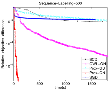
Refer to caption
(a) Relative Objective Difference
Refer to caption
(b) Non-zero Parameters
Figure 3: Sequence Labeling Problem for λ=500𝜆500\lambda=500
Refer to caption
(a) Relative Objective Difference
Refer to caption
(b) Non-zero Parameters
Figure 4: Sequence Labeling Problem for λ=50𝜆50\lambda=50

E.1.2 Hierarchical Classification
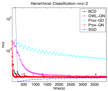
Refer to caption
(a) Relative Objective Difference
Refer to caption
(b) Non-zero Parameters
Figure 5: Hierarchical Classification Problem for λ=2𝜆2\lambda=2
Refer to caption
(a) Relative Objective Difference
Refer to caption
(b) Non-zero Parameters
Figure 6: Hierarchical Classification Problem for λ=0.5𝜆0.5\lambda=0.5

E.2 Testing Accuracy

The testing accuracy for different λ𝜆\lambda’s on these two problems is in the following tables. The testing accuracy across training time is shown in Figure 7.

λ𝜆\lambda 50 100 500
Testing Accuracy 0.834928 0.736643 0.407895
nnz of optimum 2542 1544 223
Table 1: Per-character testing accuracy for OCR dataset
λ𝜆\lambda 0.5 1 2
Testing Accuracy 0.262648 0.249731 0.185684
nnz of optimum 28483 4301 1505
Table 2: Testing accuracy for LSHTC1 dataset
Refer to caption
(a) OCR dataset with λ=100𝜆100\lambda=100
Refer to caption
(b) LSHTC1 dataset with λ=1𝜆1\lambda=1
Figure 7: Testing accuracy v.s. training time

E.3 Relative objective difference v.s. the number of passes over dataset

Figure 8 shows the performance under the measure of number of passes (iterations) over dataset. We do not include the plot for BCD method, because the pass over dataset for BCD actually depends on the sparsity pattern of the dataset. Thus it is hard to fairly define the pass over dataset for BCD. In this experiment, shrinking strategy is not applied.
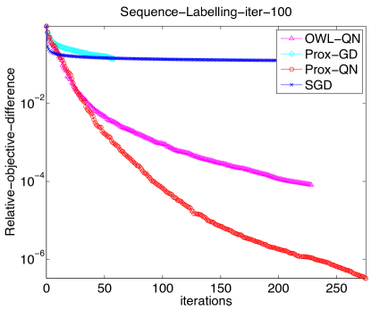
Refer to caption
Figure 8: Relative objective difference v.s. the number of passes over dataset for OCR dataset with λ=100𝜆100\lambda=100.