\@IEEEtunefonts

Diversity versus Multiplexing at Finite Blocklength

Johan Östman1, Wei Yang1, Giuseppe Durisi1, Tobias Koch2
1Chalmers University of Technology, 41296 Gothenburg, Sweden
2Universidad Carlos III de Madrid, 28911 Leganés, Spain
Abstract

A finite blocklenth analysis of the diversity-multiplexing tradeoff is presented, based on nonasymptotic bounds on the maximum channel coding rate of multiple-antenna block-memoryless Rayleigh-fading channels. The bounds in this paper allow one to numerically assess for which packet size, number of antennas, and degree of channel selectivity, diversity-exploiting schemes are close to optimal, and when instead the available spatial degrees of freedom should be used to provide spatial multiplexing. This finite blocklength view on the diversity-multiplexing tradeoff provides insights on the design of delay-sensitive ultra-reliable communication links. This research was supported by the Swedish Research Council under grant 2012-4571, by a Marie Curie FP7 Integration Grant within the 7th European Union Framework Programme under Grant 333680, and by the Spanish Government (CSD2008-00010, TEC2009-14504-C02-01, and TEC2013-41718-R).

I Introduction

Multi-antenna technology is by now a fundamental part of all modern wireless communication standards, due to its ability to provide impressive gains in both spectral efficiency and reliability. Multiple antennas yield additional spatial degrees of freedom that can be used to lower the error probability for a given rate, through the exploitation of spatial diversity, or increase the rate for a given error probability, through the exploitation of spatial multiplexing. These two effects cannot be harvested concurrently and there exists a fundamental tradeoff between diversity and multiplexing. This tradeoff admits a particularly simple characterization in the regime of high signal-to-noise ratio (SNR) and infinitely long data packets (codewords) [1].

Current cellular systems operate typically at maximum multiplexing [2]. Indeed, diversity-exploiting techniques such as space-time codes turn out to be detrimental for low-mobility users, for which the fading coefficients can be learnt easily at the transmitter and outage events can be avoided altogether by rate adaptation. On the other hand, for high-mobility users, diversity-exploiting techniques are not advantageous because of the abundant time and frequency selectivity that is available. These considerations hold under the assumptions of long packet lengths (100010001000 channel uses or more) and moderately low packet error probability (around 102superscript10210^{-2}).

As we move towards next generation wireless communication systems (5G), these assumptions may cease to be valid. Emerging applications in 5G (such as metering, traffic safety, and telecontrol of industrial plants) may require the exchange of short packets, sometimes under stringent latency and reliability constraints [3, 4]. The question addressed in this paper is how multiple antennas should be used in this scenario. Is diversity more beneficial than multiplexing in the regime of short packet length (say 100100100 channel uses, roughly equal to a LTE resource block) and high reliability (packet error rate equal to 105superscript10510^{-5} or lower)? What is the cost of learning the fading coefficients, which is required to exploit spatial degrees of freedom, when the packet size is short? Does this cost overcome the benefits of multiple antennas?111In the infinite blocklength regime, this question was addressed in [5, 6]. In this paper, we shed light on these questions leveraging on recent progresses in finite blocklength information theory [7, 8, 9].

Notation

Upper case letters such as X𝑋X denote scalar random variables and their realizations are written in lower case, e.g., x𝑥x. We use boldface upper case letters to denote random vectors, e.g., 𝑿𝑿\bm{X}, and boldface lower case letters for their realizations, e.g., 𝒙𝒙\bm{x}. Upper case letters of two special fonts are used to denote deterministic matrices (e.g., 𝖸𝖸\mathsf{Y}) and random matrices (e.g., \use@mathgroup\M@U\symAMSbY\use@mathgroup\M@U\symAMSb𝑌\use@mathgroup\M@U\symAMSb{Y}). The superscript H stands for Hermitian transposition and we use tr()tr\mathrm{tr}\mathopen{}\left(\cdot\right) and det()det\mathrm{det}\mathopen{}\left(\cdot\right) to denote the trace and the determinant of a given matrix, respectively. The identity matrix of size a×a𝑎𝑎a\times a is written as 𝖨asubscript𝖨𝑎\mathsf{I}_{a}. The distribution of a circularly symmetric complex Gaussian random variable with variance σ2superscript𝜎2\sigma^{2} is denoted by 𝒞𝒩(0,σ2)𝒞𝒩0superscript𝜎2\mathcal{CN}\mathopen{}\left(0,\sigma^{2}\right). Finally, ln()\ln(\cdot) indicates the natural logarithm, [a]+superscriptdelimited-[]𝑎[a]^{+} stands for max{a,0}𝑎0\max\{a,0\}, and Γα(β)subscriptΓ𝛼𝛽\Gamma_{\alpha}\mathopen{}\left(\beta\right) denotes the complex multivariate Gamma function.

II Channel Model and Performance Metrics

We consider a Rayleigh block-fading channel with Mtsubscript𝑀tM_{\text{{}t}} transmit antennas and Mrsubscript𝑀rM_{\text{{}r}} receive antennas that stays constant for T𝑇T channel uses. For a frequency-flat narrowband channel, T𝑇T is the number of channel uses in time over which the channel stays constant (coherence time); for a frequency-selective channel and under the assumption that orthogonal frequency-division multiplexing (OFDM) is used, T𝑇T is the number of subcarriers over which the channel stays constant (coherence bandwidth). More generally, T𝑇T can be interpreted as the number of “time-frequency slots” over which the channel does not change. Within the l𝑙lth coherence interval, the channel input-output relation can be written as

\use@mathgroup\M@U\symAMSbYl=ρ/Mt𝖷l\use@mathgroup\M@U\symAMSbHl+\use@mathgroup\M@U\symAMSbWl.\use@mathgroup\M@U\symAMSbsubscript𝑌𝑙𝜌subscript𝑀tsubscript𝖷𝑙\use@mathgroup\M@U\symAMSbsubscript𝐻𝑙\use@mathgroup\M@U\symAMSbsubscript𝑊𝑙\displaystyle\use@mathgroup\M@U\symAMSb{Y}_{l}=\sqrt{{\rho}/{M_{\text{{}t}}}}\mathsf{X}_{l}\use@mathgroup\M@U\symAMSb{H}_{l}+\use@mathgroup\M@U\symAMSb{W}_{l}. (1)

Here, 𝖷l\use@mathgroup\M@U\symAMSbCT×Mtsubscript𝖷𝑙\use@mathgroup\M@U\symAMSbsuperscript𝐶𝑇subscript𝑀t\mathsf{X}_{l}\in\use@mathgroup\M@U\symAMSb{C}^{T\times M_{\text{{}t}}} and \use@mathgroup\M@U\symAMSbYl\use@mathgroup\M@U\symAMSbCT×Mr\use@mathgroup\M@U\symAMSbsubscript𝑌𝑙\use@mathgroup\M@U\symAMSbsuperscript𝐶𝑇subscript𝑀r\use@mathgroup\M@U\symAMSb{Y}_{l}\in\use@mathgroup\M@U\symAMSb{C}^{T\times M_{\text{{}r}}} are the transmitted and received matrices, respectively; the entries of the complex fading matrix \use@mathgroup\M@U\symAMSbHl\use@mathgroup\M@U\symAMSbCMt×Mr\use@mathgroup\M@U\symAMSbsubscript𝐻𝑙\use@mathgroup\M@U\symAMSbsuperscript𝐶subscript𝑀tsubscript𝑀r\use@mathgroup\M@U\symAMSb{H}_{l}\in\use@mathgroup\M@U\symAMSb{C}^{M_{\text{{}t}}\times M_{\text{{}r}}} are independent and identically distributed (i.i.d.) 𝒞𝒩(0,1)𝒞𝒩01\mathcal{CN}\mathopen{}\left(0,1\right); \use@mathgroup\M@U\symAMSbWl\use@mathgroup\M@U\symAMSbCT×Mr\use@mathgroup\M@U\symAMSbsubscript𝑊𝑙\use@mathgroup\M@U\symAMSbsuperscript𝐶𝑇subscript𝑀r\use@mathgroup\M@U\symAMSb{W}_{l}\in\use@mathgroup\M@U\symAMSb{C}^{T\times M_{\text{{}r}}} denotes the additive noise at the receiver and has i.i.d. 𝒞𝒩(0,1)𝒞𝒩01\mathcal{CN}\mathopen{}\left(0,1\right) entries. We assume {\use@mathgroup\M@U\symAMSbHl}\use@mathgroup\M@U\symAMSbsubscript𝐻𝑙\left\{\use@mathgroup\M@U\symAMSb{H}_{l}\right\} and {\use@mathgroup\M@U\symAMSbWl}\use@mathgroup\M@U\symAMSbsubscript𝑊𝑙\left\{\use@mathgroup\M@U\symAMSb{W}_{l}\right\} to take on independent realizations over successive coherence intervals. We further assume that \use@mathgroup\M@U\symAMSbHl\use@mathgroup\M@U\symAMSbsubscript𝐻𝑙\use@mathgroup\M@U\symAMSb{H}_{l} and \use@mathgroup\M@U\symAMSbWl\use@mathgroup\M@U\symAMSbsubscript𝑊𝑙\use@mathgroup\M@U\symAMSb{W}_{l} are independent and that their joint law does not depend on 𝖷lsubscript𝖷𝑙\mathsf{X}_{l}.

Throughout the paper, we shall focus on the so called noncoherent setting where both the transmitter and the receiver know the distribution of \use@mathgroup\M@U\symAMSbHl\use@mathgroup\M@U\symAMSbsubscript𝐻𝑙\use@mathgroup\M@U\symAMSb{H}_{l} but not its realization. In other words, a priori channel state information (CSI) is not available at transmitter and at the receiver.

The assumption of no CSI at the transmitter is reasonable in a high-mobility scenario, where the fast channel variations make channel tracking at the transmitter unfeasible. It is also appropriate for transmission over control channels or for time-critical applications. Indeed, in both situations it is desirable to avoid the creation of a feedback link, required to provide CSI at the transmitter. The assumption of no a priori CSI at the receiver allows one to characterize the information-theoretic cost of learning the channel at the receiver (for example by pilot transmission followed by channel estimation); see also [9, Sec. I]. This cost may be relevant when the packet size is limited and the channel is rapidly varying.

We consider coding schemes with blocklength n=LT𝑛𝐿𝑇n=LT. Specifically, each codeword 𝖷L[𝖷1,,𝖷L]superscript𝖷𝐿subscript𝖷1subscript𝖷𝐿\mathsf{X}^{L}\triangleq[\mathsf{X}_{1},\dots,\mathsf{X}_{L}] consists of L𝐿L subcodewords {𝖷l}l=1Lsuperscriptsubscriptsubscript𝖷𝑙𝑙1𝐿\{\mathsf{X}_{l}\}_{l=1}^{L}, each one undergoing a different fading realization. We shall refer to L𝐿L as the number of time-frequency diversity branches. It is a measure of the degree of time-frequency selectivity of the propagation channel. Furthermore, each codeword is subject to the power constraint

1Ll=1Ltr(𝖷l𝖷l𝖧)=TMt.1𝐿superscriptsubscript𝑙1𝐿trsubscript𝖷𝑙superscriptsubscript𝖷𝑙𝖧𝑇subscript𝑀t\displaystyle\frac{1}{L}\sum_{l=1}^{L}\mathrm{tr}\mathopen{}\left(\mathsf{X}_{l}\mathsf{X}_{l}^{\mathsf{H}}\right)=TM_{\text{{}t}}. (2)

Since the variance of the entries of \use@mathgroup\M@U\symAMSbHl\use@mathgroup\M@U\symAMSbsubscript𝐻𝑙\use@mathgroup\M@U\symAMSb{H}_{l} and of \use@mathgroup\M@U\symAMSbWl\use@mathgroup\M@U\symAMSbsubscript𝑊𝑙\use@mathgroup\M@U\symAMSb{W}_{l} in (1) is normalized to one, ρ𝜌\rho in (1) can be thought of as the SNR at each receive antenna.

We shall constrain the subcodewords {𝖷l}l=1Lsuperscriptsubscriptsubscript𝖷𝑙𝑙1𝐿\{\mathsf{X}_{l}\}_{l=1}^{L} to be scaled unitary matrices, i.e.,

𝖷l𝖧𝖷l=c𝖨M,l=1,,Lformulae-sequencesuperscriptsubscript𝖷𝑙𝖧subscript𝖷𝑙𝑐subscript𝖨𝑀𝑙1𝐿\displaystyle\mathsf{X}_{l}^{\mathsf{H}}\mathsf{X}_{l}=c\cdot\mathsf{I}_{M},\quad l=1,\dots,L (3)

where c𝑐c denotes a positive constant. Assumption (3) forces orthogonality in space, and the transmit power to be allocated uniformly across antennas and coherence intervals. Such a power-allocation strategy is reasonable if i) the fading process is isotropic in space and i.i.d. across coherence intervals and ii) the transmitter is not aware of the channel realizations. As we shall discuss in the next section, the assumption (3) is, for example, satisfied by unitary space-time modulation, which achieves the ergodic capacity at high SNR when TMt+Mr𝑇subscript𝑀tsubscript𝑀rT\geq M_{\text{{}t}}+M_{\text{{}r}} [10, 11].

The objective of the paper is to characterize the maximal channel coding rate R(n,ϵ)superscript𝑅𝑛italic-ϵR^{*}(n,\epsilon) among all codes that have blocklength n𝑛n, that satisfy both (2) and (3), and that are decodable with average error probability not exceeding ϵitalic-ϵ\epsilon. A formal definition of R(n,ϵ)superscript𝑅𝑛italic-ϵR^{*}(n,\epsilon) follows along the same line as [8, Def. 1].

III Outage and Ergodic Capacity

Most of the results available in the literature can be interpreted as asymptotic characterizations of R(n,ϵ)superscript𝑅𝑛italic-ϵR^{*}(n,\epsilon) for n𝑛n\to\infty. For the case when T𝑇T and, hence n𝑛n, grows to infinity for a fixed L𝐿L, the maximum coding rate R(n,ϵ)superscript𝑅𝑛italic-ϵR^{*}(n,\epsilon) converges to the outage capacity Cout,ϵsubscript𝐶outitalic-ϵC_{\mathrm{out},\epsilon} [12, p. 2631][13]

Cout,ϵ=sup{R:Pout(R)ϵ}subscript𝐶outitalic-ϵsupremumconditional-set𝑅subscript𝑃out𝑅italic-ϵ\displaystyle C_{\mathrm{out},\epsilon}=\sup\mathopen{}\left\{R:P_{\text{{}out}}(R)\leq\epsilon\right\} (4)

where Pout(R)subscript𝑃out𝑅P_{\text{{}out}}(R) is the outage probability, defined as

Pout(R)=Pr{l=1Llndet(𝖨+ρMt\use@mathgroup\M@U\symAMSbHl\use@mathgroup\M@U\symAMSbHl𝖧)<R}.subscript𝑃out𝑅Prsuperscriptsubscript𝑙1𝐿𝖨𝜌subscript𝑀t\use@mathgroup\M@U\symAMSbsubscript𝐻𝑙\use@mathgroup\M@U\symAMSbsuperscriptsubscript𝐻𝑙𝖧𝑅\displaystyle P_{\text{{}out}}(R)=\Pr\Biggl{\{}\sum_{l=1}^{L}\ln\det\Bigl{(}\mathsf{I}+\frac{\rho}{M_{\text{{}t}}}\use@mathgroup\M@U\symAMSb{H}_{l}\use@mathgroup\M@U\symAMSb{H}_{l}^{\mathsf{H}}\Bigr{)}<R\Biggr{\}}. (5)

The outage capacity does not depend on whether CSI is actually available at the receiver or not. Indeed, as the coherent interval T𝑇T increases, the cost of learning the channel at the receiver vanishes [8].

The diversity gain d(r)superscript𝑑𝑟d^{*}(r) as a function of the multiplexing gain r𝑟r (as defined in [1]) is obtained by setting R=rlnρ𝑅𝑟𝜌R=r\ln\rho in (5), and by computing the asymptotic ratio

d(r)=limρPout(rlnρ)lnρ.superscript𝑑𝑟subscript𝜌subscript𝑃out𝑟𝜌𝜌\displaystyle d^{*}(r)=-\lim_{\rho\to\infty}\frac{P_{\text{{}out}}(r\ln\rho)}{\ln\rho}. (6)

For the channel (1), the diversity d(r)superscript𝑑𝑟d^{*}(r) as a function of r𝑟r is a piecewise linear curve joining the points (k,L(Mtk)(Mrk))𝑘𝐿subscript𝑀t𝑘subscript𝑀r𝑘(k,L(M_{\text{{}t}}-k)(M_{\text{{}r}}-k)) where k=1,,min{Mt,Mr}𝑘1subscript𝑀tsubscript𝑀rk=1,\dots,\min\{M_{\text{{}t}},M_{\text{{}r}}\}. The price to be paid for such an elegant characterization of the tradeoff between diversity and multiplexing is its asymptotic nature in both the blocklength and the SNR, which may limit its significance for the scenarios analyzed in this paper.

For the case when L𝐿L, and hence n𝑛n, grows to infinity for a fixed T𝑇T, the maximum coding rate R(n,ϵ)superscript𝑅𝑛italic-ϵR^{*}(n,\epsilon) converges to the ergodic capacity Cerg(ρ)subscript𝐶erg𝜌C_{\mathrm{erg}}(\rho), which, for the case when the constraint (3) is relaxed, is given by

Cerg(ρ)=(1/T)supI(\use@mathgroup\M@U\symAMSbX;\use@mathgroup\M@U\symAMSbY)subscript𝐶erg𝜌1𝑇supremum𝐼\use@mathgroup\M@U\symAMSb𝑋\use@mathgroup\M@U\symAMSb𝑌\displaystyle C_{\mathrm{erg}}(\rho)=({1}/{T})\sup I(\use@mathgroup\M@U\symAMSb{X};\use@mathgroup\M@U\symAMSb{Y}) (7)

where \use@mathgroup\M@U\symAMSbY=ρ/Mt\use@mathgroup\M@U\symAMSbX\use@mathgroup\M@U\symAMSbH+\use@mathgroup\M@U\symAMSbW\use@mathgroup\M@U\symAMSb𝑌𝜌subscript𝑀t\use@mathgroup\M@U\symAMSb𝑋\use@mathgroup\M@U\symAMSb𝐻\use@mathgroup\M@U\symAMSb𝑊\use@mathgroup\M@U\symAMSb{Y}=\sqrt{\rho/M_{\text{{}t}}}\use@mathgroup\M@U\symAMSb{X}\use@mathgroup\M@U\symAMSb{H}+\use@mathgroup\M@U\symAMSb{W} and the supremum is over all probability distributions of T×Mt𝑇subscript𝑀tT\times M_{\text{{}t}} matrices \use@mathgroup\M@U\symAMSbX\use@mathgroup\M@U\symAMSb𝑋\use@mathgroup\M@U\symAMSb{X} satisfying \use@mathgroup\M@U\symAMSbE[tr(\use@mathgroup\M@U\symAMSbX\use@mathgroup\M@U\symAMSbX𝖧)]TMt\use@mathgroup\M@U\symAMSb𝐸delimited-[]tr\use@mathgroup\M@U\symAMSb𝑋\use@mathgroup\M@U\symAMSbsuperscript𝑋𝖧𝑇subscript𝑀t\use@mathgroup\M@U\symAMSb{E}\mathopen{}\left[\mathrm{tr}\mathopen{}\left(\use@mathgroup\M@U\symAMSb{X}\use@mathgroup\M@U\symAMSb{X}^{\mathsf{H}}\right)\right]\leq TM_{\text{{}t}}. A closed-form expression for (7) is not available. It is known that choosing \use@mathgroup\M@U\symAMSbX\use@mathgroup\M@U\symAMSb𝑋\use@mathgroup\M@U\symAMSb{X} to be an isotropically distributed scaled unitary matrix achieves the first two terms in the high-SNR expansion of Cerg(ρ)subscript𝐶erg𝜌C_{\mathrm{erg}}(\rho) for the case when TMt+Mr𝑇subscript𝑀tsubscript𝑀rT\geq M_{\text{{}t}}+M_{\text{{}r}} [10, 11]. Such an input distribution, which is often referred to as unitary space-time modulation (USTM), yields codewords satisfying (3). This result thus provides support for introducing the additional codeword constraint (3). In the remainder of the paper, we shall focus on the case TMt+Mr𝑇subscript𝑀tsubscript𝑀rT\geq M_{\text{{}t}}+M_{\text{{}r}} and denote the USTM input distribution by P\use@mathgroup\M@U\symAMSbXUsuperscriptsubscript𝑃\use@mathgroup\M@U\symAMSb𝑋UP_{\use@mathgroup\M@U\symAMSb{X}}^{\mathrm{U}}.

IV Bounds on R(n,ϵ)superscript𝑅𝑛italic-ϵR^{*}(n,\epsilon)

IV-A Output distribution induced by USTM

A fundamental ingredient of the nonasymptotic bounds on R(n,ϵ)superscript𝑅𝑛italic-ϵR^{*}(n,\epsilon) described in this section is the following closed-form expression for the probability density function (pdf) induced on the channel output \use@mathgroup\M@U\symAMSbY=ρ/Mt\use@mathgroup\M@U\symAMSbX\use@mathgroup\M@U\symAMSbH+\use@mathgroup\M@U\symAMSbW\use@mathgroup\M@U\symAMSb𝑌𝜌subscript𝑀t\use@mathgroup\M@U\symAMSb𝑋\use@mathgroup\M@U\symAMSb𝐻\use@mathgroup\M@U\symAMSb𝑊\use@mathgroup\M@U\symAMSb{Y}=\sqrt{\rho/M_{\text{{}t}}}\use@mathgroup\M@U\symAMSb{X}\use@mathgroup\M@U\symAMSb{H}+\use@mathgroup\M@U\symAMSb{W} by a USTM-distributed input \use@mathgroup\M@U\symAMSbXP\use@mathgroup\M@U\symAMSbXUsimilar-to\use@mathgroup\M@U\symAMSb𝑋superscriptsubscript𝑃\use@mathgroup\M@U\symAMSb𝑋U\use@mathgroup\M@U\symAMSb{X}\sim P_{\use@mathgroup\M@U\symAMSb{X}}^{\mathrm{U}}.

Proposition 1

The pdf induced on \use@mathgroup\M@U\symAMSbY\use@mathgroup\M@U\symAMSb𝑌\use@mathgroup\M@U\symAMSb{Y} in (1) by an USTM input distribution P\use@mathgroup\M@U\symAMSbXUsuperscriptsubscript𝑃\use@mathgroup\M@U\symAMSb𝑋UP_{\use@mathgroup\M@U\symAMSb{X}}^{\mathrm{U}} is

f\use@mathgroup\M@U\symAMSbY(𝖸)subscript𝑓\use@mathgroup\M@U\symAMSb𝑌𝖸\displaystyle f_{\use@mathgroup\M@U\symAMSb{Y}}(\mathsf{Y}) =\displaystyle= (1+ρT/Mt)Mt(TMtMr)πMrT(ρT/Mt)Mt(TMt)superscript1𝜌𝑇subscript𝑀tsubscript𝑀t𝑇subscript𝑀tsubscript𝑀rsuperscript𝜋subscript𝑀r𝑇superscript𝜌𝑇subscript𝑀tsubscript𝑀t𝑇subscript𝑀t\displaystyle\frac{\mathopen{}\left(1+\rho T/M_{\text{{}t}}\right)^{M_{\text{{}t}}(T-M_{\text{{}t}}-M_{\text{{}r}})}}{\pi^{M_{\text{{}r}}T}(\rho T/M_{\text{{}t}})^{M_{\text{{}t}}(T-M_{\text{{}t}})}} (8)
ΓMt(T)ΓMt(Mt)φρ,Mt,T(σ12,,σMr2).absentsubscriptΓsubscript𝑀t𝑇subscriptΓsubscript𝑀tsubscript𝑀tsubscript𝜑𝜌subscript𝑀t𝑇superscriptsubscript𝜎12superscriptsubscript𝜎subscript𝑀r2\displaystyle\cdot\frac{\Gamma_{M_{\text{{}t}}}(T)}{\Gamma_{M_{\text{{}t}}}(M_{\text{{}t}})}\varphi_{\rho,M_{\text{{}t}},T}(\sigma_{1}^{2},\ldots,\sigma_{M_{\text{{}r}}}^{2}).

Here, σ1σMrsubscript𝜎1subscript𝜎subscript𝑀r\sigma_{1}\geq\cdots\geq\sigma_{M_{\text{{}r}}} denote the ordered singular values of 𝖸𝖸\mathsf{Y}, and φρ,Mt,T:\use@mathgroup\M@U\symAMSbR+Mr\use@mathgroup\M@U\symAMSbR+:subscript𝜑𝜌subscript𝑀t𝑇\use@mathgroup\M@U\symAMSbsubscriptsuperscript𝑅subscript𝑀r\use@mathgroup\M@U\symAMSbsubscript𝑅\varphi_{\rho,M_{\text{{}t}},T}:\use@mathgroup\M@U\symAMSb{R}^{M_{\text{{}r}}}_{+}\to\use@mathgroup\M@U\symAMSb{R}_{+} is defined as

φρ,Mt,T(b1,,bMr)subscript𝜑𝜌subscript𝑀t𝑇subscript𝑏1subscript𝑏subscript𝑀r\displaystyle\varphi_{\rho,M_{\text{{}t}},T}(b_{1},\ldots,b_{M_{\text{{}r}}}) \displaystyle\triangleq det𝖠i<jMr(bibj)𝖠subscriptsuperscriptproductsubscript𝑀r𝑖𝑗subscript𝑏𝑖subscript𝑏𝑗\displaystyle\frac{\det\mathsf{A}}{\prod\nolimits^{M_{\text{{}r}}}_{i<j}(b_{i}-b_{j})} (9)
i=1Mre(1+ρT/Mt)1bibiTMr\displaystyle\cdot\prod\limits_{i=1}^{M_{\text{{}r}}}\frac{e^{-(1+\rho T/M_{\text{{}t}})^{-1}b_{i}}}{b_{i}^{T-M_{\text{{}r}}}}

where 𝖠𝖠\mathsf{A} is an Mr×Mrsubscript𝑀rsubscript𝑀rM_{\text{{}r}}\times M_{\text{{}r}} real matrix whose (j,k)𝑗𝑘(j,k)th entry is

[𝖠]jk={bkMtjγ~(T+j2Mt,ρTbkMt+ρT), if LMtbkTjexp[bkρT/(Mt+ρT)],otherwisesubscriptdelimited-[]𝖠𝑗𝑘casessuperscriptsubscript𝑏𝑘subscript𝑀t𝑗~𝛾𝑇𝑗2subscript𝑀t𝜌𝑇subscript𝑏𝑘subscript𝑀t𝜌𝑇 if 𝐿subscript𝑀tsuperscriptsubscript𝑏𝑘𝑇𝑗subscript𝑏𝑘𝜌𝑇subscript𝑀t𝜌𝑇otherwise\displaystyle[\mathsf{A}]_{jk}=\begin{cases}b_{k}^{M_{\text{{}t}}-j}\tilde{\gamma}\mathopen{}\left(T+j-2M_{\text{{}t}},\frac{\rho Tb_{k}}{M_{\text{{}t}}+\rho T}\right),&\,\text{ if }L\leq M_{\text{{}t}}\\ b_{k}^{T-j}\exp\mathopen{}\left[-b_{k}\rho T/(M_{\text{{}t}}+\rho T)\right],&\,\text{otherwise}\end{cases} (10)

with

γ~(n,x)1Γ(n)0xtn1et𝑑t~𝛾𝑛𝑥1Γ𝑛superscriptsubscript0𝑥superscript𝑡𝑛1superscript𝑒𝑡differential-d𝑡\tilde{\gamma}(n,x)\triangleq\frac{1}{\Gamma(n)}\int\nolimits_{0}^{x}t^{n-1}e^{-t}dt (11)

denoting the regularized incomplete Gamma function.

Proof:

See [14]. ∎

Remark 1

A different expression for the output pdf induced by P\use@mathgroup\M@U\symAMSbXUsubscriptsuperscript𝑃U\use@mathgroup\M@U\symAMSb𝑋P^{\mathrm{U}}_{\use@mathgroup\M@U\symAMSb{X}} is reported in [15]. The expression in Proposition 1 appears to be easier to compute and more stable numerically.

IV-B USTM Dependency Testing Lower Bound

We first present a lower bound on R(n,ϵ)superscript𝑅𝑛italic-ϵR^{*}(n,\epsilon) that is based on the dependency testing (DT) bound developed in [7, Th. 17] and makes use of the USTM input distribution.

Theorem 2

Let \use@mathgroup\M@U\symAMSbZl\use@mathgroup\M@U\symAMSbsubscript𝑍𝑙\use@mathgroup\M@U\symAMSb{Z}_{l}, l=1,,L𝑙1𝐿l=1,\ldots,L, be independent complex Gaussian T×Mr𝑇subscript𝑀rT\times M_{\text{{}r}} matrices with i.i.d. 𝒞𝒩(0,1)𝒞𝒩01\mathcal{CN}(0,1) entries. Let Λl,1Λl,MrsubscriptΛ𝑙1subscriptΛ𝑙subscript𝑀r\Lambda_{l,1}\geq\ldots\geq\Lambda_{l,M_{\text{{}r}}} denote the ordered eigenvalues of \use@mathgroup\M@U\symAMSbZ𝖧𝖣\use@mathgroup\M@U\symAMSbZ\use@mathgroup\M@U\symAMSbsuperscript𝑍𝖧𝖣\use@mathgroup\M@U\symAMSb𝑍\use@mathgroup\M@U\symAMSb{Z}^{\mathsf{H}}\mathsf{D}\use@mathgroup\M@U\symAMSb{Z}, where 𝖣\use@mathgroup\M@U\symAMSbRT×T𝖣\use@mathgroup\M@U\symAMSbsuperscript𝑅𝑇𝑇\mathsf{D}\in\use@mathgroup\M@U\symAMSb{R}^{T\times T} is given by

𝖣=diag{1+ρT/Mt,,1+ρT/MtMt,1,,1TMt}.𝖣diagsubscript1𝜌𝑇subscript𝑀t1𝜌𝑇subscript𝑀tsubscript𝑀tsubscript11𝑇subscript𝑀t\displaystyle\mathsf{D}=\mathrm{diag}\mathopen{}\Big{\{}\underbrace{1+\rho T/M_{\text{{}t}},...,1+\rho T/M_{\text{{}t}}}_{M_{\text{{}t}}},\underbrace{1,...,1}_{T-M_{\text{{}t}}}\Big{\}}. (12)

Let

Slsubscript𝑆𝑙\displaystyle S_{l} \displaystyle\triangleq cMt,Ttr(\use@mathgroup\M@U\symAMSbZl𝖧\use@mathgroup\M@U\symAMSbZl)lnφρ,Mt,T(Λl,1,,Λl,Mr)subscript𝑐subscript𝑀t𝑇tr\use@mathgroup\M@U\symAMSbsuperscriptsubscript𝑍𝑙𝖧\use@mathgroup\M@U\symAMSbsubscript𝑍𝑙subscript𝜑𝜌subscript𝑀t𝑇subscriptΛ𝑙1subscriptΛ𝑙subscript𝑀r\displaystyle c_{M_{\text{{}t}},T}-\,\mathrm{tr}\mathopen{}\left(\use@mathgroup\M@U\symAMSb{Z}_{l}^{\mathsf{H}}\use@mathgroup\M@U\symAMSb{Z}_{l}\right)-\ln\varphi_{\rho,M_{\text{{}t}},T}(\Lambda_{l,1},\ldots,\Lambda_{l,M_{\text{{}r}}}) (13)

where

cMt,TMt(TMt)lnρTMt+ρTlnΓMt(T)ΓMt(Mt)subscript𝑐subscript𝑀t𝑇subscript𝑀t𝑇subscript𝑀t𝜌𝑇subscript𝑀t𝜌𝑇subscriptΓsubscript𝑀t𝑇subscriptΓsubscript𝑀tsubscript𝑀t\displaystyle c_{M_{\text{{}t}},T}\triangleq M_{\text{{}t}}(T-M_{\text{{}t}})\ln\frac{\rho T}{M_{\text{{}t}}+\rho T}-\ln\frac{\Gamma_{M_{\text{{}t}}}(T)}{\Gamma_{M_{\text{{}t}}}(M_{\text{{}t}})} (14)

and φρ,Mt,T:\use@mathgroup\M@U\symAMSbR+Mr\use@mathgroup\M@U\symAMSbR+:subscript𝜑𝜌subscript𝑀t𝑇\use@mathgroup\M@U\symAMSbsubscriptsuperscript𝑅subscript𝑀r\use@mathgroup\M@U\symAMSbsubscript𝑅\varphi_{\rho,M_{\text{{}t}},T}:\use@mathgroup\M@U\symAMSb{R}^{M_{\text{{}r}}}_{+}\to\use@mathgroup\M@U\symAMSb{R}_{+} is defined in (9). Furthermore, let

ϵub(n,M)\use@mathgroup\M@U\symAMSbE[exp{[l=1LSllnM12]+}].subscriptitalic-ϵub𝑛𝑀\use@mathgroup\M@U\symAMSb𝐸delimited-[]superscriptdelimited-[]superscriptsubscript𝑙1𝐿subscript𝑆𝑙𝑀12\displaystyle\epsilon_{\mathrm{ub}}(n,M)\triangleq\use@mathgroup\M@U\symAMSb{E}\mathopen{}\left[\exp\mathopen{}\left\{-\Biggl{[}\sum\limits_{l=1}^{L}S_{l}-\ln\frac{M-1}{2}\Biggr{]}^{+}\right\}\right]. (15)

We have

R(n,ϵ)max{(lnM)/n:ϵub(n,M)ϵ}.superscript𝑅𝑛italic-ϵ:𝑀𝑛subscriptitalic-ϵub𝑛𝑀italic-ϵ\displaystyle R^{*}(n,\epsilon)\geq\max\mathopen{}\left\{{(\ln M)}/{n}:\epsilon_{\mathrm{ub}}(n,M)\leq\epsilon\right\}. (16)
Proof:

The lower bound (16) follows by applying the DT bound [7, Th. 17] with an input distribution P\use@mathgroup\M@U\symAMSbXLUsubscriptsuperscript𝑃U\use@mathgroup\M@U\symAMSbsuperscript𝑋𝐿P^{\mathrm{U}}_{\use@mathgroup\M@U\symAMSb{X}^{L}} chosen so that the subcodewords {\use@mathgroup\M@U\symAMSbXl}l=1Lsuperscriptsubscript\use@mathgroup\M@U\symAMSbsubscript𝑋𝑙𝑙1𝐿\{\use@mathgroup\M@U\symAMSb{X}_{l}\}_{l=1}^{L}, are i.i.d. P\use@mathgroup\M@U\symAMSbXUsuperscriptsubscript𝑃\use@mathgroup\M@U\symAMSb𝑋UP_{\use@mathgroup\M@U\symAMSb{X}}^{\mathrm{U}}-distributed. Let f\use@mathgroup\M@U\symAMSbYLsubscript𝑓\use@mathgroup\M@U\symAMSbsuperscript𝑌𝐿f_{\use@mathgroup\M@U\symAMSb{Y}^{L}} denote the pdf of \use@mathgroup\M@U\symAMSbYL\use@mathgroup\M@U\symAMSbsuperscript𝑌𝐿\use@mathgroup\M@U\symAMSb{Y}^{L} induced by P\use@mathgroup\M@U\symAMSbXLUsubscriptsuperscript𝑃U\use@mathgroup\M@U\symAMSbsuperscript𝑋𝐿P^{\mathrm{U}}_{\use@mathgroup\M@U\symAMSb{X}^{L}}, and f\use@mathgroup\M@U\symAMSbYL|\use@mathgroup\M@U\symAMSbXLsubscript𝑓conditional\use@mathgroup\M@U\symAMSbsuperscript𝑌𝐿\use@mathgroup\M@U\symAMSbsuperscript𝑋𝐿f_{\use@mathgroup\M@U\symAMSb{Y}^{L}\,|\,\use@mathgroup\M@U\symAMSb{X}^{L}} denote the conditional pdf of \use@mathgroup\M@U\symAMSbYL\use@mathgroup\M@U\symAMSbsuperscript𝑌𝐿\use@mathgroup\M@U\symAMSb{Y}^{L} given \use@mathgroup\M@U\symAMSbXL\use@mathgroup\M@U\symAMSbsuperscript𝑋𝐿\use@mathgroup\M@U\symAMSb{X}^{L}. To use the DT bound [7, Th. 17], we need to compute the information density

ıL(𝖷L;𝖸L)lnf\use@mathgroup\M@U\symAMSbYL|\use@mathgroup\M@U\symAMSbXL(𝖸L|𝖷L)f\use@mathgroup\M@U\symAMSbYL(𝖸L).subscriptitalic-ı𝐿superscript𝖷𝐿superscript𝖸𝐿subscript𝑓conditional\use@mathgroup\M@U\symAMSbsuperscript𝑌𝐿\use@mathgroup\M@U\symAMSbsuperscript𝑋𝐿conditionalsuperscript𝖸𝐿superscript𝖷𝐿subscript𝑓\use@mathgroup\M@U\symAMSbsuperscript𝑌𝐿superscript𝖸𝐿\displaystyle\imath_{L}\mathopen{}\left(\mathsf{X}^{L};\mathsf{Y}^{L}\right)\triangleq\ln\frac{f_{\use@mathgroup\M@U\symAMSb{Y}^{L}\,|\,\use@mathgroup\M@U\symAMSb{X}^{L}}(\mathsf{Y}^{L}\,|\,\mathsf{X}^{L})}{f_{\use@mathgroup\M@U\symAMSb{Y}^{L}}(\mathsf{Y}^{L})}. (17)

Since the channel (1) is block-memoryless, f\use@mathgroup\M@U\symAMSbYL|\use@mathgroup\M@U\symAMSbXL(𝖸L|𝖷L)subscript𝑓conditional\use@mathgroup\M@U\symAMSbsuperscript𝑌𝐿\use@mathgroup\M@U\symAMSbsuperscript𝑋𝐿conditionalsuperscript𝖸𝐿superscript𝖷𝐿f_{\use@mathgroup\M@U\symAMSb{Y}^{L}\,|\,\use@mathgroup\M@U\symAMSb{X}^{L}}(\mathsf{Y}^{L}\,|\,\mathsf{X}^{L}) factorizes as l=1Lf\use@mathgroup\M@U\symAMSbY|\use@mathgroup\M@U\symAMSbX(𝖸l|𝖷l)superscriptsubscriptproduct𝑙1𝐿subscript𝑓conditional\use@mathgroup\M@U\symAMSb𝑌\use@mathgroup\M@U\symAMSb𝑋conditionalsubscript𝖸𝑙subscript𝖷𝑙\prod_{l=1}^{L}f_{\use@mathgroup\M@U\symAMSb{Y}\,|\,\use@mathgroup\M@U\symAMSb{X}}(\mathsf{Y}_{l}\,|\,\mathsf{X}_{l}) with

f\use@mathgroup\M@U\symAMSbY|\use@mathgroup\M@U\symAMSbX(𝖸|𝖷)=etr(𝖸𝖧(ρMt1𝖷𝖷𝖧+𝖨T)1𝖸)πMrTdet(ρMt1𝖷𝖷𝖧+𝖨T)Mr.subscript𝑓conditional\use@mathgroup\M@U\symAMSb𝑌\use@mathgroup\M@U\symAMSb𝑋conditional𝖸𝖷superscript𝑒trsuperscript𝖸𝖧superscript𝜌superscriptsubscript𝑀t1superscript𝖷𝖷𝖧subscript𝖨𝑇1𝖸superscript𝜋subscript𝑀r𝑇superscript𝜌superscriptsubscript𝑀t1superscript𝖷𝖷𝖧subscript𝖨𝑇subscript𝑀r\displaystyle f_{\use@mathgroup\M@U\symAMSb{Y}\,|\,\use@mathgroup\M@U\symAMSb{X}}(\mathsf{Y}\,|\,\mathsf{X})=\frac{e^{-\mathrm{tr}\mathopen{}\left(\mathsf{Y}^{\mathsf{H}}\bigl{(}\rho M_{\text{{}t}}^{-1}\mathsf{X}\mathsf{X}^{\mathsf{H}}+\mathsf{I}_{T}\bigr{)}^{-1}\mathsf{Y}\right)}}{\pi^{M_{\text{{}r}}T}\det(\rho M_{\text{{}t}}^{-1}\mathsf{X}\mathsf{X}^{\mathsf{H}}+\mathsf{I}_{T})^{M_{\text{{}r}}}}. (18)

Moreover, since the {\use@mathgroup\M@U\symAMSbXl}l=1Lsuperscriptsubscript\use@mathgroup\M@U\symAMSbsubscript𝑋𝑙𝑙1𝐿\{\use@mathgroup\M@U\symAMSb{X}_{l}\}_{l=1}^{L} are i.i.d., f\use@mathgroup\M@U\symAMSbYLsubscript𝑓\use@mathgroup\M@U\symAMSbsuperscript𝑌𝐿f_{\use@mathgroup\M@U\symAMSb{Y}^{L}} also factorizes as

f\use@mathgroup\M@U\symAMSbYL(𝖸L)=l=1Lf\use@mathgroup\M@U\symAMSbY(𝖸l)subscript𝑓\use@mathgroup\M@U\symAMSbsuperscript𝑌𝐿superscript𝖸𝐿superscriptsubscriptproduct𝑙1𝐿subscript𝑓\use@mathgroup\M@U\symAMSb𝑌subscript𝖸𝑙\displaystyle f_{\use@mathgroup\M@U\symAMSb{Y}^{L}}(\mathsf{Y}^{L})=\prod_{l=1}^{L}f_{\use@mathgroup\M@U\symAMSb{Y}}(\mathsf{Y}_{l}) (19)

where f\use@mathgroup\M@U\symAMSbYsubscript𝑓\use@mathgroup\M@U\symAMSb𝑌f_{\use@mathgroup\M@U\symAMSb{Y}} is given in (8). It thus follows that

ıL(𝖷L,𝖸L)=l=1Lı(𝖷l;𝖸l)subscriptitalic-ı𝐿superscript𝖷𝐿superscript𝖸𝐿superscriptsubscript𝑙1𝐿italic-ısubscript𝖷𝑙subscript𝖸𝑙\displaystyle\imath_{L}(\mathsf{X}^{L},\mathsf{Y}^{L})=\sum\limits_{l=1}^{L}\imath(\mathsf{X}_{l};\mathsf{Y}_{l}) (20)

where

ı(𝖷;𝖸)=lnf\use@mathgroup\M@U\symAMSbY|\use@mathgroup\M@U\symAMSbX(𝖸|𝖷)f\use@mathgroup\M@U\symAMSbY(𝖸).italic-ı𝖷𝖸subscript𝑓conditional\use@mathgroup\M@U\symAMSb𝑌\use@mathgroup\M@U\symAMSb𝑋conditional𝖸𝖷subscript𝑓\use@mathgroup\M@U\symAMSb𝑌𝖸\displaystyle\imath(\mathsf{X};\mathsf{Y})=\ln\frac{f_{\use@mathgroup\M@U\symAMSb{Y}\,|\,\use@mathgroup\M@U\symAMSb{X}}(\mathsf{Y}\,|\,\mathsf{X})}{f_{\use@mathgroup\M@U\symAMSb{Y}}(\mathsf{Y})}. (21)

Since P\use@mathgroup\M@U\symAMSbYUsubscriptsuperscript𝑃U\use@mathgroup\M@U\symAMSb𝑌P^{\mathrm{U}}_{\use@mathgroup\M@U\symAMSb{Y}} is isotropic, the probability distribution of ı(𝖷l;\use@mathgroup\M@U\symAMSbYl)italic-ısubscript𝖷𝑙\use@mathgroup\M@U\symAMSbsubscript𝑌𝑙\imath\mathopen{}\left(\mathsf{X}_{l};\use@mathgroup\M@U\symAMSb{Y}_{l}\right) takes the same value for all subcodeword matrices 𝖷lsubscript𝖷𝑙\mathsf{X}_{l} satisfying (3). Without loss of generality, we choose 𝖷l=𝖷¯subscript𝖷𝑙¯𝖷\mathsf{X}_{l}=\bar{\mathsf{X}}, l=1,,L𝑙1𝐿l=1,\ldots,L, where

𝖷¯[T𝖨Mt𝟎].¯𝖷delimited-[]𝑇subscript𝖨subscript𝑀t0\displaystyle\bar{\mathsf{X}}\triangleq\left[\begin{array}[]{c}\sqrt{T}\mathsf{I}_{M_{\text{{}t}}}\\ \mathbf{0}\\ \end{array}\right]. (24)

Through algebraic manipulations, one can show that, under P\use@mathgroup\M@U\symAMSbYL|\use@mathgroup\M@U\symAMSbXL=𝖷¯Lsubscript𝑃conditional\use@mathgroup\M@U\symAMSbsuperscript𝑌𝐿\use@mathgroup\M@U\symAMSbsuperscript𝑋𝐿superscript¯𝖷𝐿P_{\use@mathgroup\M@U\symAMSb{Y}^{L}\,|\,\use@mathgroup\M@U\symAMSb{X}^{L}=\bar{\mathsf{X}}^{L}}, the random variable ı(𝖷¯l;\use@mathgroup\M@U\symAMSbYl)italic-ısubscript¯𝖷𝑙\use@mathgroup\M@U\symAMSbsubscript𝑌𝑙\imath\mathopen{}\left(\bar{\mathsf{X}}_{l};\use@mathgroup\M@U\symAMSb{Y}_{l}\right) has the same distribution as Slsubscript𝑆𝑙S_{l}. Hence, ıL(𝖷¯L;\use@mathgroup\M@U\symAMSbYL)subscriptitalic-ı𝐿superscript¯𝖷𝐿\use@mathgroup\M@U\symAMSbsuperscript𝑌𝐿\imath_{L}\mathopen{}\left(\bar{\mathsf{X}}^{L};\use@mathgroup\M@U\symAMSb{Y}^{L}\right) has the same distribution as l=1LSlsuperscriptsubscript𝑙1𝐿subscript𝑆𝑙\sum\nolimits_{l=1}^{L}S_{l}. This proves (16). ∎

IV-C Meta-converse Upper Bound

We next establish an upper bound on R(n,ϵ)superscript𝑅𝑛italic-ϵR^{*}(n,\epsilon).

Theorem 3

Let the random variables {\use@mathgroup\M@U\symAMSbY¯l\use@mathgroup\M@U\symAMSbCT×Mr}subscript¯\use@mathgroup\M@U\symAMSb𝑌𝑙\use@mathgroup\M@U\symAMSbsuperscript𝐶𝑇subscript𝑀r\{\bar{\use@mathgroup\M@U\symAMSb{Y}}_{l}\in\use@mathgroup\M@U\symAMSb{C}^{T\times M_{\text{{}r}}}\}, l=1,,L𝑙1𝐿l=1,\ldots,L, be i.i.d. P\use@mathgroup\M@U\symAMSbYUsubscriptsuperscript𝑃U\use@mathgroup\M@U\symAMSb𝑌P^{\mathrm{U}}_{\use@mathgroup\M@U\symAMSb{Y}}-distributed; let Δl,1,,Δl,MrsubscriptΔ𝑙1subscriptΔ𝑙subscript𝑀r\Delta_{l,1},\ldots,\Delta_{l,M_{\text{{}r}}} denote the nonzero singular values of \use@mathgroup\M@U\symAMSbY¯lsubscript¯\use@mathgroup\M@U\symAMSb𝑌𝑙\bar{\use@mathgroup\M@U\symAMSb{Y}}_{l}, and let Δldiag(Δl,1,,Δl,Mr)subscriptdouble-struck-Δ𝑙diagsubscriptΔ𝑙1subscriptΔ𝑙subscript𝑀r\mathbb{\Delta}_{l}\triangleq\mathrm{diag}\left(\Delta_{l,1},\ldots,\Delta_{l,M_{\text{{}r}}}\right). Further let {\use@mathgroup\M@U\symAMSbUl\use@mathgroup\M@U\symAMSbCT×Mt}\use@mathgroup\M@U\symAMSbsubscript𝑈𝑙\use@mathgroup\M@U\symAMSbsuperscript𝐶𝑇subscript𝑀t\{\use@mathgroup\M@U\symAMSb{U}_{l}\in\use@mathgroup\M@U\symAMSb{C}^{T\times M_{\text{{}t}}}\}, l=1,,L𝑙1𝐿l=1,\ldots,L, be i.i.d. isotropically distributed unitary matrices; let 𝖣𝖣\mathsf{D}Slsubscript𝑆𝑙S_{l}cMt,Tsubscript𝑐subscript𝑀t𝑇c_{M_{\text{{}t}},T}, and φρ,Mt,Tsubscript𝜑𝜌subscript𝑀t𝑇\varphi_{\rho,M_{\text{{}t}},T} be defined as in (12), (13), (14), and (9), respectively. Finally, let

Klsubscript𝐾𝑙\displaystyle K_{l} \displaystyle\triangleq cMt,Ttr(Δl2\use@mathgroup\M@U\symAMSbUl𝖧𝖣1\use@mathgroup\M@U\symAMSbUl)subscript𝑐subscript𝑀t𝑇trsuperscriptsubscriptdouble-struck-Δ𝑙2\use@mathgroup\M@U\symAMSbsubscriptsuperscript𝑈𝖧𝑙superscript𝖣1\use@mathgroup\M@U\symAMSbsubscript𝑈𝑙\displaystyle c_{M_{\text{{}t}},T}-\mathrm{tr}\mathopen{}\left(\mathbb{\Delta}_{l}^{2}\use@mathgroup\M@U\symAMSb{U}^{\mathsf{H}}_{l}\mathsf{D}^{-1}\use@mathgroup\M@U\symAMSb{U}_{l}\right) (25)
lnφρ,Mt,T(Δl,1,,Δl,Mr).subscript𝜑𝜌subscript𝑀t𝑇subscriptΔ𝑙1subscriptΔ𝑙subscript𝑀r\displaystyle-\,\ln\varphi_{\rho,M_{\text{{}t}},T}(\Delta_{l,1},\ldots,\Delta_{l,M_{\text{{}r}}}).

Then, for every n𝑛n and every 0<ϵ<10italic-ϵ10<\epsilon<1, the maximal channel coding rate R(n,ϵ)superscript𝑅𝑛italic-ϵR^{*}(n,\epsilon) for the block-memoryless Rayleigh-fading channel (1) is upper-bounded by

R(n,ϵ)1nln1\use@mathgroup\M@U\symAMSbP[l=1LKlnγn]superscript𝑅𝑛italic-ϵ1𝑛1\use@mathgroup\M@U\symAMSb𝑃delimited-[]superscriptsubscript𝑙1𝐿subscript𝐾𝑙𝑛subscript𝛾𝑛\displaystyle R^{*}(n,\epsilon)\leq\frac{1}{n}\ln\frac{1}{\use@mathgroup\M@U\symAMSb{P}\mathopen{}\big{[}\sum\nolimits_{l=1}^{L}K_{l}\geq n\gamma_{n}\big{]}} (26)

where γnsubscript𝛾𝑛\gamma_{n} is the solution of

\use@mathgroup\M@U\symAMSbP[l=1LSlnγn]=ϵ.\use@mathgroup\M@U\symAMSb𝑃delimited-[]superscriptsubscript𝑙1𝐿subscript𝑆𝑙𝑛subscript𝛾𝑛italic-ϵ\displaystyle\use@mathgroup\M@U\symAMSb{P}\mathopen{}\biggl{[}\sum_{l=1}^{L}S_{l}\leq n\gamma_{n}\biggr{]}=\epsilon. (27)
Remark 2

The conditional probability \use@mathgroup\M@U\symAMSbP[l=1LKlnγn|{Δl}]\use@mathgroup\M@U\symAMSb𝑃delimited-[]superscriptsubscript𝑙1𝐿subscript𝐾𝑙conditional𝑛subscript𝛾𝑛subscriptdouble-struck-Δ𝑙\use@mathgroup\M@U\symAMSb{P}\mathopen{}\big{[}\sum\nolimits_{l=1}^{L}K_{l}\geq n\gamma_{n}|\{\mathbb{\Delta}_{l}\}\big{]} can be computed in closed-form by evaluating the conditional characteristic function of Klsubscript𝐾𝑙K_{l} given Δlsubscriptdouble-struck-Δ𝑙\mathbb{\Delta}_{l} using the Itzykson-Zuber integral formula [16, Eq. (3.4)].

Proof:

To upper-bound R(n,ϵ)superscript𝑅𝑛italic-ϵR^{*}(n,\epsilon), we use the meta-converse (MC) bound [7, Th. 28] with the following auxiliary distribution

Q\use@mathgroup\M@U\symAMSbYL=l=1LP\use@mathgroup\M@U\symAMSbYU.subscript𝑄\use@mathgroup\M@U\symAMSbsuperscript𝑌𝐿superscriptsubscriptproduct𝑙1𝐿subscriptsuperscript𝑃U\use@mathgroup\M@U\symAMSb𝑌\displaystyle Q_{\use@mathgroup\M@U\symAMSb{Y}^{L}}=\prod\limits_{l=1}^{L}P^{\mathrm{U}}_{\use@mathgroup\M@U\symAMSb{Y}}. (28)

Since P\use@mathgroup\M@U\symAMSbYUsubscriptsuperscript𝑃U\use@mathgroup\M@U\symAMSb𝑌P^{\mathrm{U}}_{\use@mathgroup\M@U\symAMSb{Y}} is isotropically distributed, β1ϵ(P\use@mathgroup\M@U\symAMSbYL|\use@mathgroup\M@U\symAMSbXL=𝖷L,Q\use@mathgroup\M@U\symAMSbYL)subscript𝛽1italic-ϵsubscript𝑃conditional\use@mathgroup\M@U\symAMSbsuperscript𝑌𝐿\use@mathgroup\M@U\symAMSbsuperscript𝑋𝐿superscript𝖷𝐿subscript𝑄\use@mathgroup\M@U\symAMSbsuperscript𝑌𝐿\beta_{1-\epsilon}(P_{\use@mathgroup\M@U\symAMSb{Y}^{L}\,|\,\use@mathgroup\M@U\symAMSb{X}^{L}=\mathsf{X}^{L}},Q_{\use@mathgroup\M@U\symAMSb{Y}^{L}}) (as defined in [7, p. 2316]) takes the same value for all 𝖷Lsuperscript𝖷𝐿\mathsf{X}^{L} satisfying (3). Thus, the MC bound yields [7, Th. 28]

R(n,ϵ)1nln1β1ϵ(P\use@mathgroup\M@U\symAMSbYL|\use@mathgroup\M@U\symAMSbXL=𝖷¯L,Q\use@mathgroup\M@U\symAMSbYL)superscript𝑅𝑛italic-ϵ1𝑛1subscript𝛽1italic-ϵsubscript𝑃conditional\use@mathgroup\M@U\symAMSbsuperscript𝑌𝐿\use@mathgroup\M@U\symAMSbsuperscript𝑋𝐿superscript¯𝖷𝐿subscript𝑄\use@mathgroup\M@U\symAMSbsuperscript𝑌𝐿\displaystyle R^{*}(n,\epsilon)\leq\frac{1}{n}\ln\frac{1}{\beta_{1-\epsilon}(P_{\use@mathgroup\M@U\symAMSb{Y}^{L}\,|\,\use@mathgroup\M@U\symAMSb{X}^{L}=\bar{\mathsf{X}}^{L}},Q_{\use@mathgroup\M@U\symAMSb{Y}^{L}})} (29)

where 𝖷¯L=[𝖷¯,,𝖷¯]superscript¯𝖷𝐿¯𝖷¯𝖷\bar{\mathsf{X}}^{L}=[\bar{\mathsf{X}},\dots,\bar{\mathsf{X}}], with 𝖷¯¯𝖷\bar{\mathsf{X}} given in (24). By the Neyman-Pearson lemma,

β1ϵ(P\use@mathgroup\M@U\symAMSbYL|\use@mathgroup\M@U\symAMSbXL=𝖷¯L,Q\use@mathgroup\M@U\symAMSbYL)=Q\use@mathgroup\M@U\symAMSbYL[ıL(𝖷¯L;\use@mathgroup\M@U\symAMSbYL)nγn]subscript𝛽1italic-ϵsubscript𝑃conditional\use@mathgroup\M@U\symAMSbsuperscript𝑌𝐿\use@mathgroup\M@U\symAMSbsuperscript𝑋𝐿superscript¯𝖷𝐿subscript𝑄\use@mathgroup\M@U\symAMSbsuperscript𝑌𝐿subscript𝑄\use@mathgroup\M@U\symAMSbsuperscript𝑌𝐿delimited-[]subscriptitalic-ı𝐿superscript¯𝖷𝐿\use@mathgroup\M@U\symAMSbsuperscript𝑌𝐿𝑛subscript𝛾𝑛\displaystyle\beta_{1-\epsilon}(P_{\use@mathgroup\M@U\symAMSb{Y}^{L}\,|\,\use@mathgroup\M@U\symAMSb{X}^{L}=\bar{\mathsf{X}}^{L}},Q_{\use@mathgroup\M@U\symAMSb{Y}^{L}})=Q_{\use@mathgroup\M@U\symAMSb{Y}^{L}}[\imath_{L}(\bar{\mathsf{X}}^{L};\use@mathgroup\M@U\symAMSb{Y}^{L})\geq n\gamma_{n}] (30)

where ıL(,)subscriptitalic-ı𝐿\imath_{L}(\cdot,\cdot) is defined in (17) and γnsubscript𝛾𝑛\gamma_{n} is the solution of

P\use@mathgroup\M@U\symAMSbYL|\use@mathgroup\M@U\symAMSbXL=𝖷¯L[ıL(𝖷¯L;\use@mathgroup\M@U\symAMSbYL)nγn]=ϵ.subscript𝑃conditional\use@mathgroup\M@U\symAMSbsuperscript𝑌𝐿\use@mathgroup\M@U\symAMSbsuperscript𝑋𝐿superscript¯𝖷𝐿delimited-[]subscriptitalic-ı𝐿superscript¯𝖷𝐿\use@mathgroup\M@U\symAMSbsuperscript𝑌𝐿𝑛subscript𝛾𝑛italic-ϵ\displaystyle P_{\use@mathgroup\M@U\symAMSb{Y}^{L}\,|\,\use@mathgroup\M@U\symAMSb{X}^{L}=\bar{\mathsf{X}}^{L}}\mathopen{}\big{[}\imath_{L}(\bar{\mathsf{X}}^{L};\use@mathgroup\M@U\symAMSb{Y}^{L})\leq n\gamma_{n}\big{]}=\epsilon. (31)

We conclude the proof by noting that, under Q\use@mathgroup\M@U\symAMSbYLsubscript𝑄\use@mathgroup\M@U\symAMSbsuperscript𝑌𝐿Q_{\use@mathgroup\M@U\symAMSb{Y}^{L}}, the random variable ıL(𝖷¯L;\use@mathgroup\M@U\symAMSbYL)subscriptitalic-ı𝐿superscript¯𝖷𝐿\use@mathgroup\M@U\symAMSbsuperscript𝑌𝐿\imath_{L}(\bar{\mathsf{X}}^{L};\use@mathgroup\M@U\symAMSb{Y}^{L}) has the same distribution as l=1LKlsuperscriptsubscript𝑙1𝐿subscript𝐾𝑙\sum\nolimits_{l=1}^{L}K_{l}, and under P\use@mathgroup\M@U\symAMSbYL|\use@mathgroup\M@U\symAMSbXL=𝖷¯Lsubscript𝑃conditional\use@mathgroup\M@U\symAMSbsuperscript𝑌𝐿\use@mathgroup\M@U\symAMSbsuperscript𝑋𝐿superscript¯𝖷𝐿P_{\use@mathgroup\M@U\symAMSb{Y}^{L}\,|\,\use@mathgroup\M@U\symAMSb{X}^{L}=\bar{\mathsf{X}}^{L}}, it has the same distribution as l=1LSlsuperscriptsubscript𝑙1𝐿subscript𝑆𝑙\sum\nolimits_{l=1}^{L}S_{l}. ∎

V Numerical Results

We consider the same setup as in [2], which is based on the 3GPP LTE standard [17]. Specifically, the packet length is set to n=168𝑛168n=168 symbols (an LTE resource block). Throughout, we set ρ=6𝜌6\rho=6 dB.

Control signaling

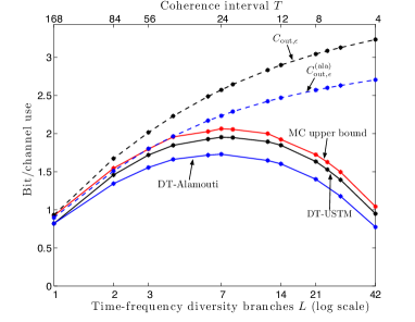
We first consider the case where the packet error rate is ϵ=103italic-ϵsuperscript103\epsilon=10^{-3}, which may be appropriate for the exchange of short packets carrying control signaling. In Fig. 1, we plot the DT lower bound (16) and the MC upper bound (26) for the case Mt=Mr=2subscript𝑀tsubscript𝑀r2M_{\text{{}t}}=M_{\text{{}r}}=2 as a function of the coherence interval T𝑇T.

Refer to caption
Figure 1: Mt=Mr=2subscript𝑀tsubscript𝑀r2M_{\text{{}t}}=M_{\text{{}r}}=2, n=168𝑛168n=168, ϵ=103italic-ϵsuperscript103\epsilon=10^{-3}.
Refer to caption
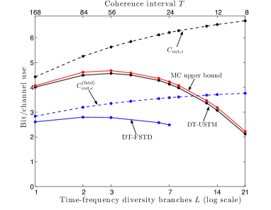
Figure 2: Mt=Mr=4subscript𝑀tsubscript𝑀r4M_{\text{{}t}}=M_{\text{{}r}}=4, n=168𝑛168n=168, ϵ=103italic-ϵsuperscript103\epsilon=10^{-3}.

These bounds describe R(n,ϵ)superscript𝑅𝑛italic-ϵR^{*}(n,\epsilon) accurately and demonstrate that R(n,ϵ)superscript𝑅𝑛italic-ϵR^{*}(n,\epsilon) is not monotonic in the coherence interval T𝑇T, but that there exists an optimal value Tsuperscript𝑇T^{*} (or equivalently, an optimal number L=n/Tsuperscript𝐿𝑛superscript𝑇L^{*}=n/T^{*} of time-frequency diversity branches) that maximizes it. For T<T𝑇superscript𝑇T<T^{*}, the cost of estimating the channel overcomes the gain due to time-frequency diversity. For T>T𝑇superscript𝑇T>T^{*}, the bottleneck is the limited time-frequency diversity offered by the channel. A similar observation was reported in [9] for the single-antenna case.

In the figure, we also plot the outage capacity Cout,ϵsubscript𝐶outitalic-ϵC_{\mathrm{out},\epsilon} in (4) as a function of the number of time-frequency diversity branches L=n/T𝐿𝑛𝑇L=n/T (with n=168𝑛168n=168). As shown in the figure, the outage capacity provides a good approximation for R(n,ϵ)superscript𝑅𝑛italic-ϵR^{*}(n,\epsilon) only when Tn𝑇𝑛T\approx n, i.e., when the fading channel is essentially constant over the duration of the packet (quasi-static scenario). Furthermore, Cout,ϵsubscript𝐶outitalic-ϵC_{\mathrm{out},\epsilon} fails to capture the loss in throughput due to channel estimation overhead, which is relevant for small T𝑇T.

The two additional curves in Fig. 1 correspond to the case of Alamouti transmission [18], a scheme that provides diversity gain 444 but no multiplexing gain [19, Sec. 9.1.5]. Both a DT bound (not detailed here for space limitations) and the outage-versus-achievable rate Cout,ϵ(ala)subscriptsuperscript𝐶alaoutitalic-ϵC^{(\mathrm{ala})}_{\mathrm{out},\epsilon} of this scheme are depicted. Fig. 1 demonstrates that, if outage capacity is used as performance metric, then a diversity-exploiting scheme such as the Alamouti code is nearly optimal when the channel provides limited diversity in time and frequency (L1𝐿1L\approx 1). However, if the channel provides significant time-frequency diversity, then one should use the antennas in multiplexing mode. For example, for the case L=14𝐿14L=14, the gap between the Alamouti scheme and the outage-optimal scheme is about 0.50.50.5 bit/channel use. Furthermore, this gap increases as L𝐿L grows. This observation is one of the key contributions of [2].

The picture changes when the limited packet size is accounted for. When L𝐿L is large, and hence T𝑇T is small, the cost of learning the channel is significant. This means that large multiplexing gains are not feasible and the gap to optimality of the Alamouti scheme decreases. For example, the throughput reduction due to the use of the Alamouti scheme (evaluated comparing the DT-Alamouti and the DT-USTM lower bounds) is about 00 bit/channel use for L=1𝐿1L=1; 0.250.250.25 bit/channel use for L=12𝐿12L=12; and 0.180.180.18 bit/channel use for L=42𝐿42L=42.

In Fig. 2, we present a similar comparison for the case of a 4×4444\times 4 system. As no generalization of the Alamouti scheme exists beyond the 2×2222\times 2 configuration [20], we consider instead the combination of Alamouti and Frequency Switched Transmit Diversity (FSTD) used in LTE [17, Sec. 11.2.2.1]. This scheme provides diversity gain 888 and no multiplexing gain. As shown in the figure, the gap between the MC upper bound and the DT-USTM lower bound is small, allowing for a precise characterization of R(n,ϵ)superscript𝑅𝑛italic-ϵR^{*}(n,\epsilon). In contrast, the gap between the DT-USTM and the DT-FSTD lower bound is large, which suggests that using all 888 antennas to provide diversity gain is suboptimal also when the time-frequency diversity is limited (i.e., L𝐿L is small).

Ultra reliable communication

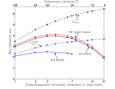
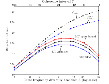
In Fig. 3 and Fig. 4, we consider the case ϵ=105italic-ϵsuperscript105\epsilon=10^{-5}, which may be relevant for the transmission of critical information, e.g., in traffic-safety applications [3].
Refer to caption
Figure 3: Mt=Mr=2subscript𝑀tsubscript𝑀r2M_{\text{{}t}}=M_{\text{{}r}}=2, n=168𝑛168n=168, ϵ=105italic-ϵsuperscript105\epsilon=10^{-5}.
Refer to caption
Figure 4: Mt=Mr=4subscript𝑀tsubscript𝑀r4M_{\text{{}t}}=M_{\text{{}r}}=4, n=168𝑛168n=168, ϵ=105italic-ϵsuperscript105\epsilon=10^{-5}.

Compared to the case ϵ=103italic-ϵsuperscript103\epsilon=10^{-3}, the gap between the optimal schemes and the diversity-based schemes (Alamouti for the 2×2222\times 2 configuration, and FSTD for the 4×4444\times 4 case) gets smaller. This comes as no surprise, since the higher reliability requirement makes the exploitation of transmit diversity advantageous.

References

  • [1] L. Zheng and D. Tse, “Diversity and multiplexing: a fundamental tradeoff in multiple-antenna channels,” IEEE Trans. Inf. Theory, vol. 49, no. 5, pp. 1073–1096, May 2003.
  • [2] A. Lozano and N. Jindal, “Transmit diversity vs. spatial multiplexing in modern MIMO systems,” IEEE Trans. Wireless Commun., vol. 9, no. 1, pp. 186–197, Sep. 2010.
  • [3] METIS project, Deliverable D1.1, “Scenarios, requirements and KPIs for 5G mobile and wireless system,” Tech. Rep., Apr. 2013.
  • [4] F. Boccardi, R. Heath, A. Lozano, T. Marzetta, and P. Popovski, “Five disruptive technology directions for 5G,” IEEE Commun. Mag., vol. 52, no. 2, pp. 74–80, Feb. 2014.
  • [5] A. Lapidoth and S. Shamai (Shitz), “Fading channels: How perfect need ‘perfect side information’ be?” IEEE Trans. Inf. Theory, vol. 48, no. 5, pp. 1118–1134, May 2002.
  • [6] B. Hassibi and B. M. Hochwald, “How much training is needed in multiple-antenna wireless links?” IEEE Trans. Inf. Theory, vol. 49, no. 4, pp. 951–963, Apr. 2003.
  • [7] Y. Polyanskiy, H. V. Poor, and S. Verdú, “Channel coding rate in the finite blocklength regime,” IEEE Trans. Inf. Theory, vol. 56, no. 5, pp. 2307–2359, May 2010.
  • [8] W. Yang, G. Durisi, T. Koch, and Y. Polyanskiy, “Quasi-static multiple-antenna fading channels at finite blocklength,” IEEE Trans. Inf. Theory, vol. 60, no. 7, pp. 4232–4265, Jul. 2014.
  • [9] ——, “Diversity versus channel knowledge at finite block-length,” in Proc. IEEE Inf. Theory Workshop (ITW), Lausanne, Switzerland, Sep. 2012, pp. 572–576.
  • [10] L. Zheng and D. N. C. Tse, “Communication on the Grassmann manifold: A geometric approach to the noncoherent multiple-antenna channel,” IEEE Trans. Inf. Theory, vol. 48, no. 2, pp. 359–383, Feb. 2002.
  • [11] W. Yang, G. Durisi, and E. Riegler, “On the capacity of large-MIMO block-fading channels,” IEEE J. Sel. Areas Commun., vol. 31, no. 2, pp. 117–132, Feb. 2013.
  • [12] E. Biglieri, J. G. Proakis, and S. Shamai (Shitz), “Fading channels: Information-theoretic and communications aspects,” IEEE Trans. Inf. Theory, vol. 44, no. 6, pp. 2619–2692, Oct. 1998.
  • [13] L. H. Ozarow, S. Shamai (Shitz), and A. D. Wyner, “Information theoretic considerations for cellular mobile radio,” IEEE Trans. Veh. Technol., vol. 43, no. 2, pp. 359–378, May 1994.
  • [14] J. Östman, “The tradeoff between transmit diversity and spatial multiplexing at finite blocklength,” Master’s thesis, Chalmers University of Technology, Göteborg, Sweden, Aug. 2014.
  • [15] B. Hassibi and T. L. Marzetta, “Multiple-antennas and isotropically random unitary inputs: The received signal density in closed form,” IEEE Trans. Inf. Theory, vol. 48, no. 6, pp. 1473 –1484, Jun. 2002.
  • [16] C. Itzykson and J. B. Zuber, “The planar approximation. II,” J. Math. Phys., vol. 21, pp. 411–421, 1980.
  • [17] S. Sesia, I. Toufik, and M. Baker, Eds., LTE–The UMTS long term evolution: From Theory to Practice, 2nd ed.   UK: Wiley, 2011.
  • [18] S. Alamouti, “A simple transmit diversity technique for wireless communications,” IEEE J. Sel. Areas Commun., vol. 16, no. 8, pp. 1451–1458, Oct. 1998.
  • [19] D. N. C. Tse and P. Viswanath, Fundamentals of Wireless Communication.   Cambridge, U.K.: Cambridge Univ. Press, 2005.
  • [20] V. Tarokh, H. Jafarkhani, and A. Calderbank, “Space-time block codes from orthogonal designs,” IEEE Trans. Inf. Theory, vol. 45, no. 5, pp. 1456–1467, Jul. 1999.