A Nonlinear Consensus Algorithm Derived from Statistical Physicsthanks: This research is partially supported by research grants from the ISF and from the Ela Kodesz Institute for Medical Engineering and Physical Sciences.

Michael Margaliot, Alon Raveh and Yoram Zarai M. Margaliot (corresponding author) is with the School of Electrical Engineering and the Sagol School of Neuroscience, Tel-Aviv University, Tel-Aviv 69978, Israel. E-mail: michaelm@eng.tau.ac.il
A. Raveh is with the School of Electrical Engineering, Tel-Aviv University, Tel-Aviv 69978, Israel. E-mail: ravehalon@gmail.com
Y. Zarai is with the School of Electrical Engineering, Tel-Aviv University, Tel-Aviv 69978, Israel. E-mail: yoramzar@mail.tau.ac.il
Abstract

The asymmetric simple exclusion process (ASEP) is an important model from statistical physics describing particles that hop randomly from one site to the next along an ordered lattice of sites, but only if the next site is empty. ASEP has been used to model and analyze numerous multiagent systems with local interactions ranging from ribosome flow along the mRNA to pedestrian traffic.

In ASEP with periodic boundary conditions a particle that hops from the last site returns to the first one. The mean field approximation of this model is referred to as the ribosome flow model on a ring (RFMR). We analyze the RFMR using the theory of monotone dynamical systems. We show that it admits a continuum of equilibrium points and that every trajectory converges to an equilibrium point. Furthermore, we show that it entrains to periodic transition rates between the sites.

When all the transition rates are equal all the state variables converge to the same value. Thus, the RFMR with homogeneous transition rates is a nonlinear consensus algorithm. We describe an application of this to a simple formation control problem.

Index Terms:
Nonlinear average consensus, monotone dynamical systems, first integral, asymptotic stability, ribosome flow model, entrainment, asymmetric simple exclusion process, mean field approximation.

I Introduction

Distributed multi-agent networks are receiving enormous attention. This seems to be motivated both by the theoretical challenges in analyzing systems with limited and time-varying communication between the agents, and numerous applications including mobile sensor networks and distributed aerospace systems [16]. A fundamental topic in this field is the consensus problem where all the agents need to agree on a certain quantity of interest while restricted by local communication and computation abilities. In the average-consensus problem, the goal is that all the agents end up with a common value that is the average of their initial values.

A consensus algorithm (protocol) is an interaction rule that specifies the information exchange between an agent and its neighbors in the network in order to reach a consensus among all the agents. An important class of algorithms, used for numerous applications, is based on linear interaction rules between the agents [20, 21].

In this paper, we consider an important model from statistical physics called the asymmetric simple exclusion process (ASEP). ASEP describes particles that hop along an ordered lattice of sites. The dynamics is stochastic: at each time step the particles are scanned, and every particle hops to the next site with some probability if the next site is empty. This simple exclusion principle allows modeling of the interaction between the particles. Note that in particular this prohibits overtaking between particles.

The term “asymmetric” refers to the fact that there is a preferred direction of movement. When the movement is unidirectional, some authors use the term totally asymmetric simple exclusion process (TASEP). ASEP was first proposed in 1968 [11] as a model for the movement of ribosomes along the mRNA strand during gene translation. In this context, the mRNA strand is the lattice and the ribosomes are the particles. Simple exclusion corresponds to the fact that a ribosome cannot move forward if there is another ribosome right in front of it. ASEP has become a paradigmatic model for non-equilibrium statistical mechanics [2, 1]. It is used as the standard model for gene translation [35], and has also been applied to model numerous multiagent systems with local interactions including traffic flow, kinesin traffic, the movement of ants along a trail, pedestrian dynamics and ad-hoc communication networks [24, 27].

The dynamic behavior of ASEP is sensitive to the boundary conditions. In ASEP with periodic boundary conditions the lattice is closed, so that a particle that hops from the last site returns to the first one. In particular, the number of particles on the lattice is conserved. In the open boundary conditions, the lattice boundaries are open and the first and last sites are connected to external particle reservoirs that drive the asymmetric flow of the particles along the lattice.

Recently, the mean field approximation of ASEP with open boundary conditions, called the ribosome flow model (RFM), has been analyzed using tools from systems and control theory [14, 13, 15, 33, 12, 34].

In this paper, we consider the mean field approximation of ASEP with periodic boundary conditions. This is a set of n𝑛n deterministic nonlinear first-order ordinary differential equations, where n𝑛n is the number of sites, and each state-variable describes the occupancy level in one of the sites. We refer to this system as the ribosome flow model on a ring (RFMR).

We show that the RFMR admits a continuum of equilibrium points, and that every trajectory converges to an equilibrium point. Furthermore, if the transition rates between the sites are periodic, with a common period T𝑇T, then every trajectory converges to a periodic solution with period T𝑇T. In other words, the RFMR entrains to the periodic excitation.

In the particular case where all the transition rates are equal all the state variables converge to the same value, namely, the average of all the initial values. In the RFMR, the dynamics of state-variable xisubscript𝑥𝑖x_{i} is local in the sense that it depends only on xi1subscript𝑥𝑖1x_{i-1}, xisubscript𝑥𝑖x_{i}, and xi+1subscript𝑥𝑖1x_{i+1}. In other words, information is exchanged between a site and its two nearest neighbors only. Thus, the convergence result implies that the RFMR with homogeneous transition rates is a nonlinear average consensus algorithm. One of the main contributions of this paper is simply in reinterpreting ASEP in the context of consensus algorithms. We describe an application of the theoretical results to a simple formation control problem.

The remainder of this paper is organized as follows. Section II reviews the RFMR. Section III details the main results. Section IV describes the application to formation control. The final section summarizes and describes several possible directions for further research.

We use standard notation. For an integer i𝑖iinnsubscript𝑖𝑛superscript𝑛i_{n}\in\mathbb{R}^{n} is the n𝑛n-dimensional column vector with all entries equal to i𝑖i. For a matrix M𝑀M, Msuperscript𝑀M^{\prime} denotes the transpose of M𝑀M. Let ||1:n+|\cdot|_{1}:\mathbb{R}^{n}\to\mathbb{R}_{+} denote the L1subscript𝐿1L_{1} vector norm, that is, |z|1=|z1|++|zn|subscript𝑧1subscript𝑧1subscript𝑧𝑛|z|_{1}=|z_{1}|+\dots+|z_{n}|.

II The model

The ribosome flow model on a ring (RFMR) is given by

x˙1subscript˙𝑥1\displaystyle\dot{x}_{1} =λnxn(1x1)λ1x1(1x2),absentsubscript𝜆𝑛subscript𝑥𝑛1subscript𝑥1subscript𝜆1subscript𝑥11subscript𝑥2\displaystyle=\lambda_{n}x_{n}(1-x_{1})-\lambda_{1}x_{1}(1-x_{2}),
x˙2subscript˙𝑥2\displaystyle\dot{x}_{2} =λ1x1(1x2)λ2x2(1x3),absentsubscript𝜆1subscript𝑥11subscript𝑥2subscript𝜆2subscript𝑥21subscript𝑥3\displaystyle=\lambda_{1}x_{1}(1-x_{2})-\lambda_{2}x_{2}(1-x_{3}),
x˙3subscript˙𝑥3\displaystyle\dot{x}_{3} =λ2x2(1x3)λ3x3(1x4),absentsubscript𝜆2subscript𝑥21subscript𝑥3subscript𝜆3subscript𝑥31subscript𝑥4\displaystyle=\lambda_{2}x_{2}(1-x_{3})-\lambda_{3}x_{3}(1-x_{4}),
\displaystyle\vdots
x˙n1subscript˙𝑥𝑛1\displaystyle\dot{x}_{n-1} =λn2xn2(1xn1)λn1xn1(1xn),absentsubscript𝜆𝑛2subscript𝑥𝑛21subscript𝑥𝑛1subscript𝜆𝑛1subscript𝑥𝑛11subscript𝑥𝑛\displaystyle=\lambda_{n-2}x_{n-2}(1-x_{n-1})-\lambda_{n-1}x_{n-1}(1-x_{n}),
x˙nsubscript˙𝑥𝑛\displaystyle\dot{x}_{n} =λn1xn1(1xn)λnxn(1x1).absentsubscript𝜆𝑛1subscript𝑥𝑛11subscript𝑥𝑛subscript𝜆𝑛subscript𝑥𝑛1subscript𝑥1\displaystyle=\lambda_{n-1}x_{n-1}(1-x_{n})-\lambda_{n}x_{n}(1-x_{1}). (1)

Here xi(t)subscript𝑥𝑖𝑡x_{i}(t) is the normalized occupancy level at site i𝑖i at time t𝑡t, so that xi(t)=0subscript𝑥𝑖𝑡0x_{i}(t)=0 [xi(t)=1subscript𝑥𝑖𝑡1x_{i}(t)=1] means that site i𝑖i is completely empty [full] at time t𝑡t. The transition rates λ1,,λnsubscript𝜆1subscript𝜆𝑛\lambda_{1},\dots,\lambda_{n} are all positive numbers.

To explain this model, consider the equation x˙2=λ1x1(1x2)λ2x2(1x3)subscript˙𝑥2subscript𝜆1subscript𝑥11subscript𝑥2subscript𝜆2subscript𝑥21subscript𝑥3\dot{x}_{2}=\lambda_{1}x_{1}(1-x_{2})-\lambda_{2}x_{2}(1-x_{3}). The term r12:=λ1x1(1x2)assignsubscript𝑟12subscript𝜆1subscript𝑥11subscript𝑥2r_{12}:=\lambda_{1}x_{1}(1-x_{2}) represents the flow of particles from site 111 to site 222. This is proportional to the occupancy x1subscript𝑥1x_{1} at site 111 and also to 1x21subscript𝑥21-x_{2}, i.e. the flow decreases as site 222 becomes fuller. This is a relaxed version of simple exclusion. The term r23:=λ2x2(1x3)assignsubscript𝑟23subscript𝜆2subscript𝑥21subscript𝑥3r_{23}:=\lambda_{2}x_{2}(1-x_{3}) represents the flow of particles from site 222 to site 333. The other equations are similar, with the term rn1:=λnxn(1x1)assignsubscript𝑟𝑛1subscript𝜆𝑛subscript𝑥𝑛1subscript𝑥1r_{n1}:=\lambda_{n}x_{n}(1-x_{1}) appearing both in the equations for x˙1subscript˙𝑥1\dot{x}_{1} and for x˙nsubscript˙𝑥𝑛\dot{x}_{n} due to the circular structure of the model (see Fig. 1).

Refer to caption
λ2subscript𝜆2\lambda_{2}x1subscript𝑥1x_{1}x2subscript𝑥2x_{2}λn1subscript𝜆𝑛1\lambda_{n-1}λnsubscript𝜆𝑛\lambda_{n}xnsubscript𝑥𝑛x_{n}λ1subscript𝜆1\lambda_{1}
Figure 1: Topology of the RFMR.

The RFMR encapsulates simple exclusion, unidirectional movement along the ring, and the periodic boundary condition of ASEP. This is not surprising, as the RFMR is the mean field approximation of ASEP with periodic boundary conditions (see, e.g., [1, p. R345] and [29, p. 1919]).

Note that we can write (II) succinctly as

x˙i=λi1xi1(1xi)λixi(1xi+1),i=1,,n,formulae-sequencesubscript˙𝑥𝑖subscript𝜆𝑖1subscript𝑥𝑖11subscript𝑥𝑖subscript𝜆𝑖subscript𝑥𝑖1subscript𝑥𝑖1𝑖1𝑛\dot{x}_{i}=\lambda_{i-1}x_{i-1}(1-x_{i})-\lambda_{i}x_{i}(1-x_{i+1}),\quad i=1,\dots,n,

where here and below every index is interpreted modulo n𝑛n. Note also that 0nsubscript0𝑛0_{n} [1nsubscript1𝑛1_{n}] is an equilibrium point of (II). Indeed, when all the sites are completely free [completely full] there is no movement of particles between the sites.

For our purposes, it is important to note that the RFMR is a local communication model in the sense that x˙ksubscript˙𝑥𝑘\dot{x}_{k} depends on xk1subscript𝑥𝑘1x_{k-1}, xksubscript𝑥𝑘x_{k}, and xk+1subscript𝑥𝑘1x_{k+1} only. If we regard xk(t)subscript𝑥𝑘𝑡x_{k}(t) as a data value of agent k𝑘k at time t𝑡t then updating this data according to (II) requires agent k𝑘k to communicate with agents k1𝑘1k-1 ,k𝑘k, and k+1𝑘1k+1 only.

Denote

Cn:={yn:yi[0,1],i=1,,n},assignsuperscript𝐶𝑛conditional-set𝑦superscript𝑛formulae-sequencesubscript𝑦𝑖01𝑖1𝑛C^{n}:=\{y\in\mathbb{R}^{n}:y_{i}\in[0,1],\;i=1,\dots,n\},

i.e., the closed unit cube in nsuperscript𝑛\mathbb{R}^{n}. Since the state-variables represent normalized occupancy levels, we always consider initial conditions x(0)Cn𝑥0superscript𝐶𝑛x(0)\in C^{n}. It is straightforward to verify that Cnsuperscript𝐶𝑛C^{n} is an invariant set of (II), i.e. x(0)Cn𝑥0superscript𝐶𝑛x(0)\in C^{n} implies that x(t)Cn𝑥𝑡superscript𝐶𝑛x(t)\in C^{n} for all t0𝑡0t\geq 0.

Note that (II) implies that

i=0nx˙i(t)0, for all t0,formulae-sequencesuperscriptsubscript𝑖0𝑛subscript˙𝑥𝑖𝑡0 for all 𝑡0\sum_{i=0}^{n}\dot{x}_{i}(t)\equiv 0,\text{ for all }t\geq 0,

so the total occupancy H(x):=1nxassign𝐻𝑥superscriptsubscript1𝑛𝑥H(x):=1_{n}^{\prime}x is conserved:

H(x(t))=H(x(0)),for all t0.formulae-sequence𝐻𝑥𝑡𝐻𝑥0for all 𝑡0H(x(t))=H(x(0)),\quad\text{for all }t\geq 0. (2)

In other words, the dynamics redistributes the particles between the sites, but without changing the total occupancy level.

Eq. (2) means that we can reduce the n𝑛n-dimensional RFMR into an (n1)𝑛1(n-1)-dimensional model. In particular, the RFMR with n=2𝑛2n=2 can be explicitly solved. The next example demonstrates this.

Example 1

Consider (II) with n=2𝑛2n=2, i.e.

x˙1subscript˙𝑥1\displaystyle\dot{x}_{1} =λ2x2(1x1)λ1x1(1x2),absentsubscript𝜆2subscript𝑥21subscript𝑥1subscript𝜆1subscript𝑥11subscript𝑥2\displaystyle=\lambda_{2}x_{2}(1-x_{1})-\lambda_{1}x_{1}(1-x_{2}),
x˙2subscript˙𝑥2\displaystyle\dot{x}_{2} =λ1x1(1x2)λ2x2(1x1).absentsubscript𝜆1subscript𝑥11subscript𝑥2subscript𝜆2subscript𝑥21subscript𝑥1\displaystyle=\lambda_{1}x_{1}(1-x_{2})-\lambda_{2}x_{2}(1-x_{1}). (3)

We assume that x(0)02𝑥0subscript02x(0)\not=0_{2} and x(0)12𝑥0subscript12x(0)\not=1_{2}, as these are equilibrium points of the dynamics. Let s:=x1(0)+x2(0)assign𝑠subscript𝑥10subscript𝑥20s:=x_{1}(0)+x_{2}(0). Substituting x2(t)=sx1(t)subscript𝑥2𝑡𝑠subscript𝑥1𝑡x_{2}(t)=s-x_{1}(t) in (1) yields

x˙1subscript˙𝑥1\displaystyle\dot{x}_{1} =λ2(sx1)(1x1)λ1x1(1s+x1)absentsubscript𝜆2𝑠subscript𝑥11subscript𝑥1subscript𝜆1subscript𝑥11𝑠subscript𝑥1\displaystyle=\lambda_{2}(s-x_{1})(1-x_{1})-\lambda_{1}x_{1}(1-s+x_{1})
=α2x12+α1x1+α0,absentsubscript𝛼2superscriptsubscript𝑥12subscript𝛼1subscript𝑥1subscript𝛼0\displaystyle=\alpha_{2}x_{1}^{2}+\alpha_{1}x_{1}+\alpha_{0}, (4)

where

α2subscript𝛼2\displaystyle\alpha_{2} :=λ2λ1,assignabsentsubscript𝜆2subscript𝜆1\displaystyle:=\lambda_{2}-\lambda_{1},
α1subscript𝛼1\displaystyle\alpha_{1} :=(λ1λ2)sλ1λ2,assignabsentsubscript𝜆1subscript𝜆2𝑠subscript𝜆1subscript𝜆2\displaystyle:=(\lambda_{1}-\lambda_{2})s-\lambda_{1}-\lambda_{2},
α0subscript𝛼0\displaystyle\alpha_{0} :=sλ2.assignabsent𝑠subscript𝜆2\displaystyle:=s\lambda_{2}.

If λ1=λ2subscript𝜆1subscript𝜆2\lambda_{1}=\lambda_{2} then (1) is a linear differential equation and its solution is

x1(t)=s2(1exp(2λ1t))+x1(0)exp(2λ1t),subscript𝑥1𝑡𝑠212subscript𝜆1𝑡subscript𝑥102subscript𝜆1𝑡\displaystyle x_{1}(t)=\frac{s}{2}(1-\exp(-2\lambda_{1}t))+x_{1}(0)\exp(-2\lambda_{1}t), (5)

so

x2(t)subscript𝑥2𝑡\displaystyle x_{2}(t) =sx1(t)absent𝑠subscript𝑥1𝑡\displaystyle=s-x_{1}(t)
=s2(1+exp(2λ1t))x1(0)exp(2λ1t)absent𝑠212subscript𝜆1𝑡subscript𝑥102subscript𝜆1𝑡\displaystyle=\frac{s}{2}(1+\exp(-2\lambda_{1}t))-x_{1}(0)\exp(-2\lambda_{1}t)
=s2(1exp(2λ1t))+x2(0)exp(2λ1t).absent𝑠212subscript𝜆1𝑡subscript𝑥202subscript𝜆1𝑡\displaystyle=\frac{s}{2}(1-\exp(-2\lambda_{1}t))+x_{2}(0)\exp(-2\lambda_{1}t). (6)

In particular,

limtx(t)=(s/2)12,subscript𝑡𝑥𝑡𝑠2subscript12\lim_{t\to\infty}x(t)=(s/2)1_{2}, (7)

i.e., the state-variables converge at an exponential rate to the average of their initial values.

If λ1λ2subscript𝜆1subscript𝜆2\lambda_{1}\not=\lambda_{2} then (1) is a Riccati equation and solving it yields

x1(t)=α1Δcoth(Δ(tt0)/2)2α2,subscript𝑥1𝑡subscript𝛼1Δhyperbolic-cotangentΔ𝑡subscript𝑡022subscript𝛼2x_{1}(t)=\frac{-\alpha_{1}-\sqrt{\Delta}\coth(\sqrt{\Delta}(t-t_{0})/2)}{2\alpha_{2}}, (8)

where

ΔΔ\displaystyle\Delta :=α124α2α0=(s1)2(λ1λ2)2+4λ1λ2,assignabsentsuperscriptsubscript𝛼124subscript𝛼2subscript𝛼0superscript𝑠12superscriptsubscript𝜆1subscript𝜆224subscript𝜆1subscript𝜆2\displaystyle:=\alpha_{1}^{2}-4\alpha_{2}\alpha_{0}=(s-1)^{2}(\lambda_{1}-\lambda_{2})^{2}+4\lambda_{1}\lambda_{2},
t0subscript𝑡0\displaystyle t_{0} :=2Δcoth1(2x1(0)α2+α1Δ).assignabsent2Δsuperscripthyperbolic-cotangent12subscript𝑥10subscript𝛼2subscript𝛼1Δ\displaystyle:=\frac{2}{\sqrt{\Delta}}\coth^{-1}\left(\frac{2x_{1}(0)\alpha_{2}+\alpha_{1}}{\sqrt{\Delta}}\right).

Note that since the λisubscript𝜆𝑖\lambda_{i}s are positive, Δ>0Δ0\Delta>0. Also, a straightforward calculation shows that t0subscript𝑡0t_{0} is well-defined for all x1(0)[0,1]subscript𝑥1001x_{1}(0)\in[0,1]. Note that (8) implies that

limtx(t)=12α2[α1Δ2α2s+α1+Δ].subscript𝑡𝑥𝑡12subscript𝛼2superscriptmatrixsubscript𝛼1Δ2subscript𝛼2𝑠subscript𝛼1Δ\lim_{t\to\infty}x(t)=\frac{1}{2\alpha_{2}}\begin{bmatrix}{-\alpha_{1}-\sqrt{\Delta}}&{2\alpha_{2}s+\alpha_{1}+\sqrt{\Delta}}\end{bmatrix}^{\prime}.

The identity

coth(t2Δ)1=2exp(Δt)1hyperbolic-cotangent𝑡2Δ12Δ𝑡1\coth\left(\frac{t}{2}\sqrt{\Delta}\right)-1=\frac{2}{\exp(\sqrt{\Delta}t)-1} (9)

implies that for sufficiently large values of t𝑡t the convergence is with rate exp(Δt)Δ𝑡\exp(-\sqrt{\Delta}t). Thus, the convergence rate depends on λ1subscript𝜆1\lambda_{1}, λ2subscript𝜆2\lambda_{2}, and s𝑠s.

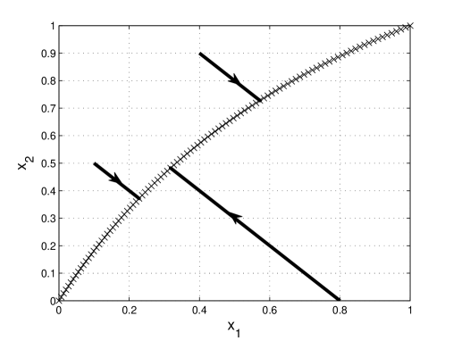
Summarizing, every trajectory follows the straight line from x(0)𝑥0x(0) to an equilibrium point e=e(λ1,λ2,s)𝑒𝑒subscript𝜆1subscript𝜆2𝑠e=e(\lambda_{1},\lambda_{2},s). In particular, if a,bC2𝑎𝑏superscript𝐶2a,b\in C^{2} satisfy 12a=12bsuperscriptsubscript12𝑎superscriptsubscript12𝑏1_{2}^{\prime}a=1_{2}^{\prime}b then the solutions emanating from a𝑎a and from b𝑏b converge to the same equilibrium point. Fig. 2 depicts the trajectories of the RFMR with n=2𝑛2n=2, λ1=2subscript𝜆12\lambda_{1}=2 and λ2=1subscript𝜆21\lambda_{2}=1 for three initial conditions. \square

Refer to caption
Figure 2: Trajectories of (II) with n=2𝑛2n=2λ1=2subscript𝜆12\lambda_{1}=2 and λ2=1subscript𝜆21\lambda_{2}=1 for three initial conditions. The dynamics admits a continuum of equilibrium points marked by ++.

The next section describes several theoretical results on the RFMR. An application of these results to a consensus problem is described in Section IV.

III Main results

III-A Strong Monotonicity

A cone K𝐾K in nsuperscript𝑛\mathbb{R}^{n} defines a partial ordering in nsuperscript𝑛\mathbb{R}^{n} as follows. For two vectors a,bn𝑎𝑏superscript𝑛a,b\in\mathbb{R}^{n}, we write ab𝑎𝑏a\leq b if (ba)K𝑏𝑎𝐾(b-a)\in K; a<b𝑎𝑏a<b if ab𝑎𝑏a\leq b and ab𝑎𝑏a\not=b; and abmuch-less-than𝑎𝑏a\ll b if (ba)Int(K)𝑏𝑎Int𝐾(b-a)\in\operatorname{Int}(K). The system y˙=f(y)˙𝑦𝑓𝑦\dot{y}=f(y) is called monotone if ab𝑎𝑏a\leq b implies that y(t,a)y(t,b)𝑦𝑡𝑎𝑦𝑡𝑏y(t,a)\leq y(t,b) for all t0𝑡0t\geq 0. In other words, the flow preserves the partial ordering [26]. It is called strongly monotone if a<b𝑎𝑏a<b implies that y(t,a)y(t,b)much-less-than𝑦𝑡𝑎𝑦𝑡𝑏y(t,a)\ll y(t,b) for all t>0𝑡0t>0.

From here on we consider the particular case where the cone is K=+n𝐾subscriptsuperscript𝑛K=\mathbb{R}^{n}_{+}. Then ab𝑎𝑏a\leq b if aibisubscript𝑎𝑖subscript𝑏𝑖a_{i}\leq b_{i} for all i𝑖i, and abmuch-less-than𝑎𝑏a\ll b if ai<bisubscript𝑎𝑖subscript𝑏𝑖a_{i}<b_{i} for all i𝑖i. A system that is monotone with respect to this partial order is called cooperative.

The linear average consensus protocol is y˙=Ay˙𝑦𝐴𝑦\dot{y}=Ay, where A𝐴A is a Metzler matrix, with zero sum rows. It is well-known that the Metzler property implies that this system is cooperative. The next result shows that the same holds for the RFMR.

Proposition 1

Let x(t,a)𝑥𝑡𝑎x(t,a) denote the solution of the RFMR at time t𝑡t for the initial condition x(0)=a𝑥0𝑎x(0)=a. For any a,bCn𝑎𝑏superscript𝐶𝑛a,b\in C^{n} with ab𝑎𝑏a\leq b we have

x(t,a)x(t,b),for all t0.formulae-sequence𝑥𝑡𝑎𝑥𝑡𝑏for all 𝑡0x(t,a)\leq x(t,b),\quad\text{for all }t\geq 0. (10)

Furthermore, if a<b𝑎𝑏a<b then

x(t,a)x(t,b),for all t>0.formulae-sequencemuch-less-than𝑥𝑡𝑎𝑥𝑡𝑏for all 𝑡0x(t,a)\ll x(t,b),\quad\text{for all }t>0. (11)

Proof. Write the RFMR (II) as x˙=f(x)˙𝑥𝑓𝑥\dot{x}=f(x). The Jacobian matrix J(x):=fx(x)assign𝐽𝑥𝑓𝑥𝑥J(x):=\frac{\partial f}{\partial x}(x) is given in (12). This matrix has nonnegative off-diagonal entries for all xCn𝑥superscript𝐶𝑛x\in C^{n}. Thus, the RFMR is a cooperative system [26], and this implies (10). Furthermore, it is straightforward to verify that J(x)𝐽𝑥J(x) is an irreducible matrix for all xCn𝑥superscript𝐶𝑛x\in C^{n}, and this implies (11) (see, e.g., [26, Ch. 4]). ∎

J(x)=[λnxnλ1(1x2)λ1x100λn(1x1)λ1(1x2)λ1x1λ2(1x3)λ2x2000λ2(1x3)λ2x2λ3(1x4)00000λn2xn2λn1(1xn)λn1xn1λnxn00λn1(1xn)λn1xn1λn(1x1)]𝐽𝑥matrixsubscript𝜆𝑛subscript𝑥𝑛subscript𝜆11subscript𝑥2subscript𝜆1subscript𝑥10missing-subexpression0subscript𝜆𝑛1subscript𝑥1subscript𝜆11subscript𝑥2subscript𝜆1subscript𝑥1subscript𝜆21subscript𝑥3subscript𝜆2subscript𝑥2missing-subexpression000subscript𝜆21subscript𝑥3subscript𝜆2subscript𝑥2subscript𝜆31subscript𝑥400missing-subexpressionmissing-subexpression000missing-subexpressionsubscript𝜆𝑛2subscript𝑥𝑛2subscript𝜆𝑛11subscript𝑥𝑛subscript𝜆𝑛1subscript𝑥𝑛1subscript𝜆𝑛subscript𝑥𝑛00missing-subexpressionsubscript𝜆𝑛11subscript𝑥𝑛subscript𝜆𝑛1subscript𝑥𝑛1subscript𝜆𝑛1subscript𝑥1J(x)=\begin{bmatrix}-\lambda_{n}x_{n}-\lambda_{1}(1-x_{2})&\lambda_{1}x_{1}&0&&0&\lambda_{n}(1-x_{1})\\ \lambda_{1}(1-x_{2})&-\lambda_{1}x_{1}-\lambda_{2}(1-x_{3})&\lambda_{2}x_{2}&&0&0\\ 0&\lambda_{2}(1-x_{3})&-\lambda_{2}x_{2}-\lambda_{3}(1-x_{4})&\dots&0&0\\ &&\vdots\\ 0&0&0&&-\lambda_{n-2}x_{n-2}-\lambda_{n-1}(1-x_{n})&\lambda_{n-1}x_{n-1}\\ \lambda_{n}x_{n}&0&0&&\lambda_{n-1}(1-x_{n})&-\lambda_{n-1}x_{n-1}-\lambda_{n}(1-x_{1})\end{bmatrix} (12)

III-B Stability

The next result shows that every level set Lssubscript𝐿𝑠L_{s} of H𝐻H contains a unique equilibrium point, and that any trajectory of the RFMR emanating from Lssubscript𝐿𝑠L_{s} converges to this equilibrium point.

Theorem 1

Pick s[0,n]𝑠0𝑛s\in[0,n], and let

Ls:={yCn:1ny=s}.assignsubscript𝐿𝑠conditional-set𝑦superscript𝐶𝑛superscriptsubscript1𝑛𝑦𝑠L_{s}:=\{y\in C^{n}:1_{n}^{\prime}y=s\}.

Then Lssubscript𝐿𝑠L_{s} contains a unique equilibrium point eLssubscript𝑒subscript𝐿𝑠e_{L_{s}} of the RFMR and for any aLs𝑎subscript𝐿𝑠a\in L_{s},

limtx(t,a)=eLs.subscript𝑡𝑥𝑡𝑎subscript𝑒subscript𝐿𝑠\lim_{t\to\infty}x(t,a)=e_{L_{s}}.

Furthermore, for any 0s<pn0𝑠𝑝𝑛0\leq s<p\leq n, we have

eLseLp.much-less-thansubscript𝑒subscript𝐿𝑠subscript𝑒subscript𝐿𝑝e_{L_{s}}\ll e_{L_{p}}. (13)

Proof. Since the RFMR is a cooperative irreducible system with H(x)=1nx𝐻𝑥superscriptsubscript1𝑛𝑥H(x)=1_{n}^{\prime}x as a first integral, Thm. 1 follows from the results in [18] (see also [17] and [8]

for some related ideas). ∎

Note that Thm. 1 implies that the RFMR has a continuum of linearly ordered equilibrium points, namely, {eLs:s[0,n]}conditional-setsubscript𝑒subscript𝐿𝑠𝑠0𝑛\{e_{L_{s}}:s\in[0,n]\}, and also that every solution of the RFMR converges to an equilibrium point.

Example 2

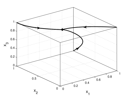
Consider the RFMR with n=3𝑛3n=3, λ1=2subscript𝜆12\lambda_{1}=2, λ2=3subscript𝜆23\lambda_{2}=3, and λ3=1subscript𝜆31\lambda_{3}=1. Fig. 3 depicts trajectories of this RFMR for three initial conditions in L2subscript𝐿2L_{2}: [1 1 0]superscriptdelimited-[]110[1\;1\;0]^{\prime}, [1 0 1]superscriptdelimited-[]101[1\;0\;1]^{\prime}, and [0 1 1]superscriptdelimited-[]011[0\;1\;1]^{\prime}. It may be observed that all the trajectories converge to the same equilibrium point eL2[0.53800.65280.8091]subscript𝑒subscript𝐿2superscriptmatrix0.53800.65280.8091e_{L_{2}}\approx\begin{bmatrix}0.5380&0.6528&0.8091\end{bmatrix}^{\prime}.

Refer to caption
Figure 3: Trajectories of (II) with n=3𝑛3n=3 for three different initial conditions in L2subscript𝐿2L_{2}: [1 1 0]superscriptdelimited-[]110[1\;1\;0]^{\prime}, [1 0 1]superscriptdelimited-[]101[1\;0\;1]^{\prime}, and [0 1 1]superscriptdelimited-[]011[0\;1\;1]^{\prime}. The equilibrium point eL2subscript𝑒subscript𝐿2e_{L_{2}} is marked with a circle.

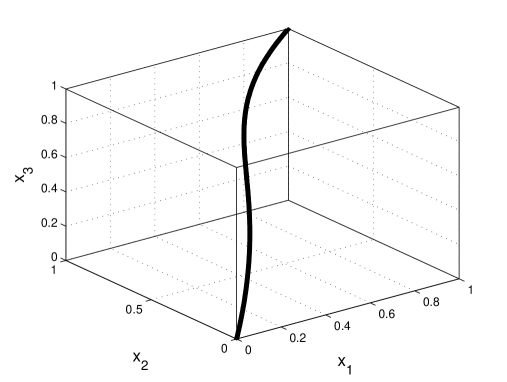
Fig. 4 depicts all the equilibrium points of this RFMR. Since λ2>λ1subscript𝜆2subscript𝜆1\lambda_{2}>\lambda_{1} and λ2>λ3subscript𝜆2subscript𝜆3\lambda_{2}>\lambda_{3}, the transition rate into site 333 is relatively large. As may be observed from the figure this leads to e3e1subscript𝑒3subscript𝑒1e_{3}\geq e_{1} and e3e2subscript𝑒3subscript𝑒2e_{3}\geq e_{2} for every equilibrium point e𝑒e\square

Refer to caption
Figure 4: All the equilibrium points of the RFMR with n=3𝑛3n=3, λ1=2subscript𝜆12\lambda_{1}=2, λ2=3subscript𝜆23\lambda_{2}=3, and λ3=1subscript𝜆31\lambda_{3}=1.
Example 3

Consider again the RFMR with n=2𝑛2n=2. Fix 0<s<p<20𝑠𝑝20<s<p<2. Pick aLs𝑎subscript𝐿𝑠a\in L_{s} and bLp𝑏subscript𝐿𝑝b\in L_{p}. If λ1=λ2subscript𝜆1subscript𝜆2\lambda_{1}=\lambda_{2} then (7) implies that

eLs=limtx(t,a)subscript𝑒subscript𝐿𝑠subscript𝑡𝑥𝑡𝑎\displaystyle e_{L_{s}}=\lim_{t\to\infty}x(t,a) =(s/2)12,absent𝑠2subscript12\displaystyle=(s/2)1_{2},
eLp=limtx(t,b)subscript𝑒subscript𝐿𝑝subscript𝑡𝑥𝑡𝑏\displaystyle e_{L_{p}}=\lim_{t\to\infty}x(t,b) =(p/2)12,absent𝑝2subscript12\displaystyle=(p/2)1_{2},

so clearly (13) holds. Now suppose that λ1λ2subscript𝜆1subscript𝜆2\lambda_{1}\not=\lambda_{2}. Assume first that λ2>λ1subscript𝜆2subscript𝜆1\lambda_{2}>\lambda_{1}. Denote the coordinates of eLssubscript𝑒subscript𝐿𝑠e_{L_{s}} [eLpsubscript𝑒subscript𝐿𝑝e_{L_{p}}] by v1subscript𝑣1v_{1}, v2subscript𝑣2v_{2} [w1subscript𝑤1w_{1}, w2subscript𝑤2w_{2}]. Recall that v1subscript𝑣1v_{1} is a root of the polynomial

Ps(z):=(λ2λ1)z2+((λ1λ2)sλ1λ2)z+sλ2assignsubscript𝑃𝑠𝑧subscript𝜆2subscript𝜆1superscript𝑧2subscript𝜆1subscript𝜆2𝑠subscript𝜆1subscript𝜆2𝑧𝑠subscript𝜆2P_{s}(z):=(\lambda_{2}-\lambda_{1})z^{2}+((\lambda_{1}-\lambda_{2})s-\lambda_{1}-\lambda_{2})z+s\lambda_{2}

(see (1)) satisfying v1[0,1]subscript𝑣101v_{1}\in[0,1]. This is a “smiling parabola” satisfying Ps(0)=sλ2>0subscript𝑃𝑠0𝑠subscript𝜆20P_{s}(0)=s\lambda_{2}>0 and Ps(1)=λ1(s2)<0subscript𝑃𝑠1subscript𝜆1𝑠20P_{s}(1)=\lambda_{1}(s-2)<0. Similarly, w1[0,1]subscript𝑤101w_{1}\in[0,1] is a root of a “smiling parabola” Pp(z)subscript𝑃𝑝𝑧P_{p}(z) satisfying Pp(0)=pλ2>0subscript𝑃𝑝0𝑝subscript𝜆20P_{p}(0)=p\lambda_{2}>0 and Pp(1)=λ1(p2)<0subscript𝑃𝑝1subscript𝜆1𝑝20P_{p}(1)=\lambda_{1}(p-2)<0. Since p>s𝑝𝑠p>s, the graph of Pp(z)subscript𝑃𝑝𝑧P_{p}(z) lies strictly above the graph of Ps(z)subscript𝑃𝑠𝑧P_{s}(z) for all z[0,1]𝑧01z\in[0,1]. Therefore, v1<w1subscript𝑣1subscript𝑤1v_{1}<w_{1}. To show that v2<w2subscript𝑣2subscript𝑤2v_{2}<w_{2} note that x2(t,a)=sx1(t,a)subscript𝑥2𝑡𝑎𝑠subscript𝑥1𝑡𝑎x_{2}(t,a)=s-x_{1}(t,a) yields

x˙2(t,a)subscript˙𝑥2𝑡𝑎\displaystyle\dot{x}_{2}(t,a) =x˙1(t,a)absentsubscript˙𝑥1𝑡𝑎\displaystyle=-\dot{x}_{1}(t,a)
=Ps(x1(t,a))absentsubscript𝑃𝑠subscript𝑥1𝑡𝑎\displaystyle=-P_{s}(x_{1}(t,a))
=Ps(sx2(t,a)).absentsubscript𝑃𝑠𝑠subscript𝑥2𝑡𝑎\displaystyle=-P_{s}(s-x_{2}(t,a)).

This implies that v2subscript𝑣2v_{2} is a root of

P¯s(z):=Ps(sz)assignsubscript¯𝑃𝑠𝑧subscript𝑃𝑠𝑠𝑧\bar{P}_{s}(z):=-P_{s}(s-z)

in [0,1]01[0,1]. This is a “frowning parabola” and a calculation yields P¯s(0)=sλ1>0subscript¯𝑃𝑠0𝑠subscript𝜆10\bar{P}_{s}(0)=s\lambda_{1}>0 and P¯s(1)=(s2)λ2<0subscript¯𝑃𝑠1𝑠2subscript𝜆20\bar{P}_{s}(1)=(s-2)\lambda_{2}<0. Now p>s𝑝𝑠p>s implies that the graph of P¯s(z)subscript¯𝑃𝑠𝑧\bar{P}_{s}(z) lies strictly below the graph of P¯p(z)subscript¯𝑃𝑝𝑧\bar{P}_{p}(z) for all z[0,1]𝑧01z\in[0,1], so v2<w2subscript𝑣2subscript𝑤2v_{2}<w_{2}. We conclude that eLseLpmuch-less-thansubscript𝑒subscript𝐿𝑠subscript𝑒subscript𝐿𝑝e_{L_{s}}\ll e_{L_{p}}. The analysis in the case λ2<λ1subscript𝜆2subscript𝜆1\lambda_{2}<\lambda_{1} is similar and again shows that (13) holds. \square

III-C Contraction

Contraction theory is a powerful tool for analyzing nonlinear dynamical systems (see, e.g., [10, 23]). In a contractive system, the distance between any two trajectories decreases at an exponential rate. It is clear that the RFMR is not a contractive system on Cnsuperscript𝐶𝑛C^{n}, with respect to any norm, as it admits more than a single equilibrium point. Nevertheless, the next result shows that the RFMR is non-expanding with respect to the L1subscript𝐿1L_{1} norm.

Proposition 2

For any a,bCn𝑎𝑏superscript𝐶𝑛a,b\in C^{n},

|x(t,a)x(t,b)|1|ab|1,for all t0.formulae-sequencesubscript𝑥𝑡𝑎𝑥𝑡𝑏1subscript𝑎𝑏1for all 𝑡0|x(t,a)-x(t,b)|_{1}\leq|a-b|_{1},\quad\text{for all }t\geq 0. (14)

In other words, the L1subscript𝐿1L_{1} distance between trajectories can never increase.

Proof. Recall that the matrix measure μ1():n×n:subscript𝜇1superscript𝑛𝑛\mu_{1}(\cdot):\mathbb{R}^{n\times n}\to\mathbb{R} induced by the L1subscript𝐿1L_{1} norm is

μ1(A)=max{c1(A),,cn(A)},subscript𝜇1𝐴subscript𝑐1𝐴subscript𝑐𝑛𝐴\mu_{1}(A)=\max\{c_{1}(A),\dots,c_{n}(A)\},

where ci(A):=aii+ki|aki|assignsubscript𝑐𝑖𝐴subscript𝑎𝑖𝑖subscript𝑘𝑖subscript𝑎𝑘𝑖c_{i}(A):=a_{ii}+\sum_{k\not=i}|a_{ki}|, i.e. the sum of entries in column i𝑖i of A𝐴A, with the off-diagonal entries taken with absolute value [31]. For the Jacobian of the RFMR, we have ci(J(x))=0subscript𝑐𝑖𝐽𝑥0c_{i}(J(x))=0 for all i𝑖i and all xCn𝑥superscript𝐶𝑛x\in C^{n}, so μ1(J(x))=0subscript𝜇1𝐽𝑥0\mu_{1}(J(x))=0. Now (14) follows from standard results in contraction theory (see, e.g., [23]). ∎

Example 4

Pick a,bCn𝑎𝑏superscript𝐶𝑛a,b\in C^{n} such that ba𝑏𝑎b\leq a. By monotonicity, x(t,b)x(t,a)𝑥𝑡𝑏𝑥𝑡𝑎x(t,b)\leq x(t,a) for all t0𝑡0t\geq 0, so d(t):=|x(t,a)x(t,b)|1=1n(x(t,a)x(t,b))assign𝑑𝑡subscript𝑥𝑡𝑎𝑥𝑡𝑏1superscriptsubscript1𝑛𝑥𝑡𝑎𝑥𝑡𝑏d(t):=|x(t,a)-x(t,b)|_{1}=1_{n}^{\prime}(x(t,a)-x(t,b)). Thus,

d˙(t)˙𝑑𝑡\displaystyle\dot{d}(t) =1nx˙(t,a)1nx˙(t,b)absentsuperscriptsubscript1𝑛˙𝑥𝑡𝑎superscriptsubscript1𝑛˙𝑥𝑡𝑏\displaystyle=1_{n}^{\prime}\dot{x}(t,a)-1_{n}^{\prime}\dot{x}(t,b)
=00,absent00\displaystyle=0-0,

so clearly in this case (14) hold with an equality. \square

Example 5

Consider the RFMR with n=2𝑛2n=2. Pick a,b(C2{02,12})𝑎𝑏superscript𝐶2subscript02subscript12a,b\in(C^{2}\setminus\{0_{2},1_{2}\}) such that s:=12a=12bassign𝑠superscriptsubscript12𝑎superscriptsubscript12𝑏s:=1_{2}^{\prime}a=1_{2}^{\prime}b. In other words, a,b𝑎𝑏a,b both belong to Lssubscript𝐿𝑠L_{s}. Note that in this case

d(t)𝑑𝑡\displaystyle d(t) :=|x1(t,a)x1(t,b)|+|x2(t,a)x2(t,b)|assignabsentsubscript𝑥1𝑡𝑎subscript𝑥1𝑡𝑏subscript𝑥2𝑡𝑎subscript𝑥2𝑡𝑏\displaystyle:=|x_{1}(t,a)-x_{1}(t,b)|+|x_{2}(t,a)-x_{2}(t,b)|
=|x1(t,a)x1(t,b)|+|sx1(t,a)(sx1(t,b))|absentsubscript𝑥1𝑡𝑎subscript𝑥1𝑡𝑏𝑠subscript𝑥1𝑡𝑎𝑠subscript𝑥1𝑡𝑏\displaystyle=|x_{1}(t,a)-x_{1}(t,b)|+|s-x_{1}(t,a)-(s-x_{1}(t,b))|
=2|x1(t,a)x1(t,b)|.absent2subscript𝑥1𝑡𝑎subscript𝑥1𝑡𝑏\displaystyle=2|x_{1}(t,a)-x_{1}(t,b)|.

In particular, d(0)=2|a1b1|𝑑02subscript𝑎1subscript𝑏1d(0)=2|a_{1}-b_{1}|. If λ1=λ2subscript𝜆1subscript𝜆2\lambda_{1}=\lambda_{2} then (5) yields d(t)=2|a1b1|exp(2λ1t),𝑑𝑡2subscript𝑎1subscript𝑏12subscript𝜆1𝑡d(t)=2|a_{1}-b_{1}|\exp(-2\lambda_{1}t), so clearly (14) holds. If λ1λ2subscript𝜆1subscript𝜆2\lambda_{1}\not=\lambda_{2} then (8) yields

d(t)=Δ|α2||coth(Δ2(tt0(b)))coth(Δ2(tt0(a)))|,𝑑𝑡Δsubscript𝛼2hyperbolic-cotangentΔ2𝑡subscript𝑡0𝑏hyperbolic-cotangentΔ2𝑡subscript𝑡0𝑎\displaystyle d(t)=\frac{\sqrt{\Delta}}{|\alpha_{2}|}\left|\coth(\frac{\sqrt{\Delta}}{2}(t-t_{0}(b)))-\coth(\frac{\sqrt{\Delta}}{2}(t-t_{0}(a)))\right|,

where t0():2:subscript𝑡0superscript2t_{0}(\cdot):\mathbb{R}^{2}\to\mathbb{R} is defined by

t0(z)subscript𝑡0𝑧\displaystyle t_{0}(z) :=2Δcoth1(2z1α2+α1Δ).assignabsent2Δsuperscripthyperbolic-cotangent12subscript𝑧1subscript𝛼2subscript𝛼1Δ\displaystyle:=\frac{2}{\sqrt{\Delta}}\coth^{-1}\left(\frac{2z_{1}\alpha_{2}+\alpha_{1}}{\sqrt{\Delta}}\right).

Applying (9) and the identity 2coth1(x)=ln(x+1x1)2superscripthyperbolic-cotangent1𝑥𝑥1𝑥12\coth^{-1}(x)=\ln(\frac{x+1}{x-1}), for |x|>1𝑥1|x|>1, yields

d(t)=d(0)/|γ(t)|,𝑑𝑡𝑑0𝛾𝑡d(t)=d(0)/|\gamma(t)|,

where

γ(t):=assign𝛾𝑡absent\displaystyle\gamma(t):= 14exp(Δt)(q(a)q(b)+1q(a)q(b))14Δ𝑡𝑞𝑎𝑞𝑏1𝑞𝑎𝑞𝑏\displaystyle\frac{1}{4}\exp(\sqrt{\Delta}t)\left(q(a)q(b)+1-q(a)-q(b)\right)
+\displaystyle+ 14exp(Δt)(q(a)q(b)+1+q(a)+q(b))14Δ𝑡𝑞𝑎𝑞𝑏1𝑞𝑎𝑞𝑏\displaystyle\frac{1}{4}\exp(-\sqrt{\Delta}t)\left(q(a)q(b)+1+q(a)+q(b)\right)
+\displaystyle+ 12(1q(a)q(b)),121𝑞𝑎𝑞𝑏\displaystyle\frac{1}{2}(1-q(a)q(b)),

and the function q():2:𝑞superscript2q(\cdot):\mathbb{R}^{2}\to\mathbb{R} is defined by

q(z):=(λ2λ1)(z1z2)(λ1+λ2)Δ.assign𝑞𝑧subscript𝜆2subscript𝜆1subscript𝑧1subscript𝑧2subscript𝜆1subscript𝜆2Δq(z):=\frac{(\lambda_{2}-\lambda_{1})(z_{1}-z_{2})-(\lambda_{1}+\lambda_{2})}{\sqrt{\Delta}}.

Note that γ(0)=1𝛾01\gamma(0)=1. We need to show that γ(t)1𝛾𝑡1\gamma(t)\geq 1 for all t0𝑡0t\geq 0, meaning

(q(a)q(b)+1)(cosh(Δt)1)(q(a)+q(b))sinh(Δt).𝑞𝑎𝑞𝑏1Δ𝑡1𝑞𝑎𝑞𝑏Δ𝑡(q(a)q(b)+1)(\cosh(\sqrt{\Delta}t)-1)\geq(q(a)+q(b))\sinh(\sqrt{\Delta}t). (15)

Since ai(0,1)subscript𝑎𝑖01a_{i}\in(0,1) and bi(0,1)subscript𝑏𝑖01b_{i}\in(0,1), q(a)<0𝑞𝑎0q(a)<0 and q(b)<0𝑞𝑏0q(b)<0. Thus (15) holds (with equality only at t=0𝑡0t=0), so γ(t)>1𝛾𝑡1\gamma(t)>1 and, therefore, d(t)<d(0)𝑑𝑡𝑑0d(t)<d(0) for all t>0𝑡0t>0\square

Pick aCn𝑎superscript𝐶𝑛a\in C^{n}, and let s:=1naassign𝑠superscriptsubscript1𝑛𝑎s:=1_{n}^{\prime}a. Substituting b=eLs𝑏subscript𝑒subscript𝐿𝑠b=e_{L_{s}} in (14) yields

|x(t,a)eLs|1|aeLs|1,for all t0.formulae-sequencesubscript𝑥𝑡𝑎subscript𝑒subscript𝐿𝑠1subscript𝑎subscript𝑒subscript𝐿𝑠1for all 𝑡0|x(t,a)-e_{L_{s}}|_{1}\leq|a-e_{L_{s}}|_{1},\quad\text{for all }t\geq 0. (16)

This means that the convergence to eLssubscript𝑒subscript𝐿𝑠e_{L_{s}} is monotone in the sense that the L1subscript𝐿1L_{1} distance to eLssubscript𝑒subscript𝐿𝑠e_{L_{s}} can never increase. Combining (16) with Theorem 1 implies that every equilibrium point of the RFMR is semistable [5].

III-D Entrainment

Consider vehicles moving along a circular road. Traffic flow is controlled by traffic lights located along the road. Assume that all the traffic lights operate at a periodic manner with a common period T>0𝑇0T>0. A natural question is: will the traffic density and/or traffic flow converge to a periodic pattern with period T𝑇T?

We can model this using the RFMR as follows. We say that a function f𝑓f is T𝑇T-periodic if f(t+T)=f(t)𝑓𝑡𝑇𝑓𝑡f(t+T)=f(t) for all t𝑡t. Assume that the λisubscript𝜆𝑖\lambda_{i}s are time-varying functions satisfying:

  • there exist 0<δ1<δ20subscript𝛿1subscript𝛿20<\delta_{1}<\delta_{2} such that λi(t)[δ1,δ2]subscript𝜆𝑖𝑡subscript𝛿1subscript𝛿2\lambda_{i}(t)\in[\delta_{1},\delta_{2}] for all t0𝑡0t\geq 0 and all i{1,,n}𝑖1𝑛i\in\{1,\dots,n\}.

  • there exists a (minimal) T>0𝑇0T>0 such that all the λisubscript𝜆𝑖\lambda_{i}s are T𝑇T-periodic.

We refer to the model in this case as the periodic ribosome flow model on a ring (PRFMR).

Theorem 2

Consider the PRFMR. Fix an arbitrary s[0,n]𝑠0𝑛s\in[0,n]. There exists a unique function ϕs:+Cn:subscriptitalic-ϕ𝑠subscriptsuperscript𝐶𝑛\phi_{s}:\mathbb{R}_{+}\to C^{n}, that is T𝑇T-periodic, and

limt|x(t,a)ϕs(t)|=0,for all aLs.formulae-sequencesubscript𝑡𝑥𝑡𝑎subscriptitalic-ϕ𝑠𝑡0for all 𝑎subscript𝐿𝑠\lim_{t\to\infty}|x(t,a)-\phi_{s}(t)|=0,\quad\text{for all }a\in L_{s}.

In other words, every level set Lssubscript𝐿𝑠L_{s} of H𝐻H contains a unique periodic solution, and every solution of the PRFMR emanating from Lssubscript𝐿𝑠L_{s} converges to this solution. Thus, the PRFMR entrains (or phase locks) to the periodic excitation in the λisubscript𝜆𝑖\lambda_{i}s.

Note that since a constant function is a periodic function for any T𝑇T, Thm. 2 implies entrainment to a periodic trajectory in the particular case where one of the λisubscript𝜆𝑖\lambda_{i}s oscillates and the other are constant. Note also that Thm. 1 follows from Thm. 2.

Proof of Thm. 2. Write the PRFMR as x˙=f(t,x)˙𝑥𝑓𝑡𝑥\dot{x}=f(t,x). Then f(t,y)=f(t+T,y)𝑓𝑡𝑦𝑓𝑡𝑇𝑦f(t,y)=f(t+T,y) for all t𝑡t and y𝑦y. Furthermore, H(x)=1nx𝐻𝑥superscriptsubscript1𝑛𝑥H(x)=1_{n}^{\prime}x is a first integral of the PRFMR. Now Thm. 2 follows from the results in [28] (see also [7]). ∎

Example 6

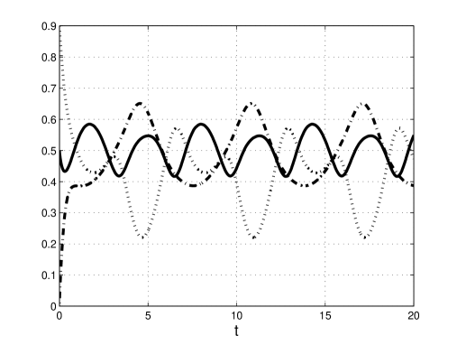
Consider the RFMR with n=3𝑛3n=3, λ1(t)=3subscript𝜆1𝑡3\lambda_{1}(t)=3, λ2(t)=3+2sin(t+1/2)subscript𝜆2𝑡32𝑡12\lambda_{2}(t)=3+2\sin(t+1/2), and λ3(t)=42cos(2t)subscript𝜆3𝑡422𝑡\lambda_{3}(t)=4-2\cos(2t). Note that all the λisubscript𝜆𝑖\lambda_{i}s are periodic with a minimal common period T=2π𝑇2𝜋T=2\pi. Fig. 5 shows the solution x(t,a)𝑥𝑡𝑎x(t,a) for a=[0.50.010.9]𝑎superscriptmatrix0.50.010.9a=\begin{bmatrix}0.5&0.01&0.9\end{bmatrix}^{\prime}. It may be seen that every xi(t)subscript𝑥𝑖𝑡x_{i}(t) converges to a periodic function with period 2π2𝜋2\pi\square

Refer to caption
Figure 5: Solution of the PRFMR in Example 6: solid line-x1(t,a)subscript𝑥1𝑡𝑎x_{1}(t,a); dash-dotted line-x2(t,a)subscript𝑥2𝑡𝑎x_{2}(t,a); dotted line-x3(t,a)subscript𝑥3𝑡𝑎x_{3}(t,a).
Example 7

Consider the RFMR with n=2𝑛2n=2λ1(t)=3q(t)/2subscript𝜆1𝑡3𝑞𝑡2\lambda_{1}(t)=3q(t)/2, and λ2(t)=q(t)/2subscript𝜆2𝑡𝑞𝑡2\lambda_{2}(t)=q(t)/2, where q(t)𝑞𝑡q(t) is a strictly positive and periodic function. Then (1) becomes

x˙1=(x12+(s2)x1+s/2)q.subscript˙𝑥1superscriptsubscript𝑥12𝑠2subscript𝑥1𝑠2𝑞\dot{x}_{1}=(-x_{1}^{2}+(s-2)x_{1}+s/2)q. (17)

Assume that

x12(0)<s/2.superscriptsubscript𝑥120𝑠2x_{1}^{2}(0)<s/2. (18)

It is straightforward to verify that in this case the solution of (17) is

x1(t)=(s/2)1+ztanh(k+z0tq(s)𝑑s),subscript𝑥1𝑡𝑠21𝑧𝑘𝑧superscriptsubscript0𝑡𝑞𝑠differential-d𝑠x_{1}(t)=(s/2)-1+z\tanh\left(k+z\int_{0}^{t}q(s)ds\right),

where

z:=3+(s1)22,assign𝑧3superscript𝑠122z:=\frac{\sqrt{3+(s-1)^{2}}}{2},

and

k:=tanh1((x1(0)+1s/2)/z).assign𝑘superscript1subscript𝑥101𝑠2𝑧k:=\tanh^{-1}\left((x_{1}(0)+1-s/2)/z\right).

Note that (18) implies that k𝑘k is well-defined. Suppose, for example, that q(t)=2+sin(t)𝑞𝑡2𝑡q(t)=2+\sin(t). Then λ1(t)subscript𝜆1𝑡\lambda_{1}(t), λ2(t)subscript𝜆2𝑡\lambda_{2}(t) are periodic with period T=2π𝑇2𝜋T=2\pi. In this case,

x1(t)=(s/2)1+ztanh(k+z(2t+1cos(t))),subscript𝑥1𝑡𝑠21𝑧𝑘𝑧2𝑡1𝑡x_{1}(t)=(s/2)-1+z\tanh\left(k+z(2t+1-\cos(t))\right),

and

x2(t)subscript𝑥2𝑡\displaystyle x_{2}(t) =sx1(t)absent𝑠subscript𝑥1𝑡\displaystyle=s-x_{1}(t)
=(s/2)+1ztanh(k+z(2t+1cos(t))).absent𝑠21𝑧𝑘𝑧2𝑡1𝑡\displaystyle=(s/2)+1-z\tanh\left(k+z(2t+1-\cos(t))\right).

Thus, for every aLs𝑎subscript𝐿𝑠a\in L_{s},  limtx(t,a)=ϕs(t)subscript𝑡𝑥𝑡𝑎subscriptitalic-ϕ𝑠𝑡\lim_{t\to\infty}x(t,a)=\phi_{s}(t), where ϕs(t)[(s/2)1+z(s/2)+1z]subscriptitalic-ϕ𝑠𝑡superscriptmatrix𝑠21𝑧𝑠21𝑧\phi_{s}(t)\equiv\begin{bmatrix}(s/2)-1+z&(s/2)+1-z\end{bmatrix}^{\prime} (which is of course periodic with period T𝑇T). \square

III-E The homogeneous case

Fix an arbitrary s[0,n]𝑠0𝑛s\in[0,n]. To simplify the notation, we just write e𝑒e instead of eLssubscript𝑒subscript𝐿𝑠e_{L_{s}} from here on. Then

1ne=s,superscriptsubscript1𝑛𝑒𝑠1_{n}^{\prime}e=s, (19)

and since for x=e𝑥𝑒x=e the left-hand side of all the equations in (II) is zero,

λnen(1e1)subscript𝜆𝑛subscript𝑒𝑛1subscript𝑒1\displaystyle\lambda_{n}e_{n}(1-{e}_{1}) =λ1e1(1e2)absentsubscript𝜆1subscript𝑒11subscript𝑒2\displaystyle=\lambda_{1}{e}_{1}(1-{e}_{2})
=λ2e2(1e3)absentsubscript𝜆2subscript𝑒21subscript𝑒3\displaystyle=\lambda_{2}{e}_{2}(1-{e}_{3})
\displaystyle\vdots
=λn1en1(1en).absentsubscript𝜆𝑛1subscript𝑒𝑛11subscript𝑒𝑛\displaystyle=\lambda_{n-1}{e}_{n-1}(1-{e}_{n}). (20)

In other words, the steady-state flow r:=rii+1=λiei(1ei+1)assign𝑟subscript𝑟𝑖𝑖1subscript𝜆𝑖subscript𝑒𝑖1subscript𝑒𝑖1r:=r_{ii+1}=\lambda_{i}{e}_{i}(1-{e}_{i+1}) for all i𝑖i.

In general, solving (19) and (III-E) explicitly seems difficult. In this section, we consider a special case where more explicit results can be derived, namely, the case where

λ1==λn:=λc,subscript𝜆1subscript𝜆𝑛assignsubscript𝜆𝑐\lambda_{1}=\dots=\lambda_{n}:=\lambda_{c},

i.e. all the transition rates are equal, with λcsubscript𝜆𝑐\lambda_{c} denoting their common value. In this case (II) becomes:

x˙1subscript˙𝑥1\displaystyle\dot{x}_{1} =λcxn(1x1)λcx1(1x2),absentsubscript𝜆𝑐subscript𝑥𝑛1subscript𝑥1subscript𝜆𝑐subscript𝑥11subscript𝑥2\displaystyle=\lambda_{c}x_{n}(1-x_{1})-\lambda_{c}x_{1}(1-x_{2}),
x˙2subscript˙𝑥2\displaystyle\dot{x}_{2} =λcx1(1x2)λcx2(1x3),absentsubscript𝜆𝑐subscript𝑥11subscript𝑥2subscript𝜆𝑐subscript𝑥21subscript𝑥3\displaystyle=\lambda_{c}x_{1}(1-x_{2})-\lambda_{c}x_{2}(1-x_{3}),
\displaystyle\vdots
x˙nsubscript˙𝑥𝑛\displaystyle\dot{x}_{n} =λcxn1(1xn)λcxn(1x1).absentsubscript𝜆𝑐subscript𝑥𝑛11subscript𝑥𝑛subscript𝜆𝑐subscript𝑥𝑛1subscript𝑥1\displaystyle=\lambda_{c}x_{n-1}(1-x_{n})-\lambda_{c}x_{n}(1-x_{1}). (21)

We refer to this as the homogeneous ribosome flow model on a ring (HRFMR). Also, (III-E) becomes

en(1e1)subscript𝑒𝑛1subscript𝑒1\displaystyle e_{n}(1-{e}_{1}) =e1(1e2)absentsubscript𝑒11subscript𝑒2\displaystyle={e}_{1}(1-{e}_{2})
=e2(1e3)absentsubscript𝑒21subscript𝑒3\displaystyle={e}_{2}(1-{e}_{3})
\displaystyle\vdots
=en1(1en),absentsubscript𝑒𝑛11subscript𝑒𝑛\displaystyle={e}_{n-1}(1-{e}_{n}), (22)

and it is straightforward to verify that e=c1n𝑒𝑐subscript1𝑛e=c1_{n}, c𝑐c\in\mathbb{R}, satisfies (III-E).

Define the averaging operator Ave():n:Avesuperscript𝑛\operatorname{Ave}(\cdot):\mathbb{R}^{n}\to\mathbb{R} by Ave(z):=1n1nzassignAve𝑧1𝑛superscriptsubscript1𝑛𝑧\operatorname{Ave}(z):=\frac{1}{n}1_{n}^{\prime}z.

Corollary 1

For any aCn𝑎superscript𝐶𝑛a\in C^{n} the solution of the HRFMR satisfies

limtx(t,a)=Ave(a)1n.subscript𝑡𝑥𝑡𝑎Ave𝑎subscript1𝑛\lim_{t\to\infty}x(t,a)=\operatorname{Ave}(a)1_{n}.

Note that this implies that the steady-state flow is r=λcAve(a)(1Ave(a))𝑟subscript𝜆𝑐Ave𝑎1Ave𝑎r=\lambda_{c}\operatorname{Ave}(a)(1-\operatorname{Ave}(a)). Thus, r𝑟r is maximized when Ave(a)=1/2Ave𝑎12\operatorname{Ave}(a)=1/2 and the maximal value is r=λc/4superscript𝑟subscript𝜆𝑐4r^{*}=\lambda_{c}/4.

Proof of Corollary 1. Let s:=1naassign𝑠superscriptsubscript1𝑛𝑎s:=1_{n}^{\prime}a. Then Lssubscript𝐿𝑠L_{s} contains Ave(a)1nAve𝑎subscript1𝑛\operatorname{Ave}(a)1_{n} and this is an equilibrium point. The proof now follows immediately from Thm. 1. ∎

Remark 1

It is possible also to give a simple and self-contained proof of Corollary 1 using standard tools from the literature on consensus networks. Indeed, pick τ>0𝜏0\tau>0 and let i𝑖i be an index such that xi(τ)xj(τ)subscript𝑥𝑖𝜏subscript𝑥𝑗𝜏x_{i}(\tau)\geq x_{j}(\tau) for all ji𝑗𝑖j\not=i. Then

x˙i(τ)subscript˙𝑥𝑖𝜏\displaystyle\dot{x}_{i}(\tau) =xi1(τ)(1xi(τ))xi(τ)(1xi+1(τ))absentsubscript𝑥𝑖1𝜏1subscript𝑥𝑖𝜏subscript𝑥𝑖𝜏1subscript𝑥𝑖1𝜏\displaystyle=x_{i-1}(\tau)(1-x_{i}(\tau))-x_{i}(\tau)(1-x_{i+1}(\tau))
xi(τ)(1xi(τ))xi(τ)(1xi(τ))absentsubscript𝑥𝑖𝜏1subscript𝑥𝑖𝜏subscript𝑥𝑖𝜏1subscript𝑥𝑖𝜏\displaystyle\leq x_{i}(\tau)(1-x_{i}(\tau))-x_{i}(\tau)(1-x_{i}(\tau))
=0.absent0\displaystyle=0.

Furthermore, if xi(τ)>xj(τ)subscript𝑥𝑖𝜏subscript𝑥𝑗𝜏x_{i}(\tau)>x_{j}(\tau) for all ji𝑗𝑖j\not=i then x˙i(τ)<0subscript˙𝑥𝑖𝜏0\dot{x}_{i}(\tau)<0. A similar argument shows that if xi(τ)xj(τ)subscript𝑥𝑖𝜏subscript𝑥𝑗𝜏x_{i}(\tau)\leq x_{j}(\tau) [xi(τ)<xj(τ)subscript𝑥𝑖𝜏subscript𝑥𝑗𝜏x_{i}(\tau)<x_{j}(\tau)] for all ji𝑗𝑖j\not=i then x˙i(τ)0subscript˙𝑥𝑖𝜏0\dot{x}_{i}(\tau)\geq 0 [x˙i(τ)>0subscript˙𝑥𝑖𝜏0\dot{x}_{i}(\tau)>0]. Define V():n+:𝑉superscript𝑛subscriptV(\cdot):\mathbb{R}^{n}\to\mathbb{R}_{+} by V(y):=maxiyiminiyiassign𝑉𝑦subscript𝑖subscript𝑦𝑖subscript𝑖subscript𝑦𝑖V(y):=\max_{i}y_{i}-\min_{i}y_{i}. Then V(x(t))𝑉𝑥𝑡V(x(t)) strictly decreases along trajectories of the HRFMR unless x(t)=c1n𝑥𝑡𝑐subscript1𝑛x(t)=c1_{n} for some c𝑐c\in\mathbb{R}, and a standard argument (see, e.g., [9]) implies that the system converges to consensus. Combining this with (2) completes the proof of Corollary 1.

In other words, the HRFMR may be interpreted as a nonlinear average consensus network. Indeed, every state-variable replaces information with its two nearest neighbors on the ring only, yet the dynamics guarantees that every state-variable converges to Ave(a)Ave𝑎\operatorname{Ave}(a).

The physical nature of the underlying model provides a simple explanation for convergence to average consensus. Indeed, the HRFMR may be interpreted as a system of n𝑛n water tanks connected in a circular topology through identical pipes. The flow in this system is driven by the imbalance in the water levels, and the state always converges to a homogeneous distribution of water in the tanks. Since the system is closed, this corresponds to average consensus.

III-E1 Convergence rate

The convergence rate of the HRFMR in the vicinity of the equilibrium point c1n𝑐subscript1𝑛c1_{n} can be analyzed as follows. Let y:=xc1nassign𝑦𝑥𝑐subscript1𝑛y:=x-c1_{n}. Then a calculation shows that the linearized dynamics of y𝑦y is given by y˙=Qy˙𝑦𝑄𝑦\dot{y}=Qy, where

Q:=[1c0001c1c1c00001c1c00c0001c1].assign𝑄matrix1𝑐0001𝑐1𝑐1𝑐00001𝑐1𝑐00𝑐0001𝑐1Q:=\begin{bmatrix}-1&c&0&0&\dots&0&1-c\\ 1-c&-1&c&0&\dots&0&0\\ 0&1-c&-1&c&\dots&0&0\\ \vdots\\ c&0&0&0&\dots&1-c&-1\\ \end{bmatrix}.

Using known-results on the eignevalues of a circulant matrix (see, e.g., [4]) implies that the eigenvalues of Q𝑄Q are

λ=1+cw1+(1c)w(1)(n1),=1,n,formulae-sequencesubscript𝜆1𝑐superscript𝑤11𝑐superscript𝑤1𝑛11𝑛\lambda_{\ell}=-1+cw^{\ell-1}+(1-c)w^{(\ell-1)(n-1)},\quad\ell=1\dots,n,

where w:=exp(2π1/n)assign𝑤2𝜋1𝑛w:=\exp(2\pi\sqrt{-1}/n). In particular, λ1=0subscript𝜆10\lambda_{1}=0. The corresponding eigenvector is 1nsubscript1𝑛1_{n}. This is a consequence of the continuum of equilibria in the HRFMR. Also,

Re(λ)Resubscript𝜆\displaystyle\operatorname{Re}(\lambda_{\ell}) =cos(2π(1)(n1)/n)absent2𝜋1𝑛1𝑛\displaystyle=\cos(2\pi(\ell-1)(n-1)/n)
+c(cos(2π(1)/n)cos(2π(1)(n1)/n))1𝑐2𝜋1𝑛2𝜋1𝑛1𝑛1\displaystyle+c(\cos(2\pi(\ell-1)/n)-\cos(2\pi(\ell-1)(n-1)/n))-1
=cos(2π(1)(n1)/n)1,absent2𝜋1𝑛1𝑛1\displaystyle=\cos(2\pi(\ell-1)(n-1)/n)-1,

and this implies that

Re(λ)Re(λ2)=cos(2π(n1)/n)1,Resubscript𝜆Resubscript𝜆22𝜋𝑛1𝑛1\displaystyle\operatorname{Re}(\lambda_{\ell})\leq\operatorname{Re}(\lambda_{2})=\cos(2\pi(n-1)/n)-1,

for =2,,n2𝑛\ell=2,\dots,n. Thus, for x(0)𝑥0x(0) in the vicinity of the equilibrium

|x(t)c1n|exp((cos(2π(n1)/n)1)t)|x(0)c1n|.𝑥𝑡𝑐subscript1𝑛2𝜋𝑛1𝑛1𝑡𝑥0𝑐subscript1𝑛|x(t)-c1_{n}|\leq\exp((\cos(2\pi(n-1)/n)-1)t)|x(0)-c1_{n}|. (23)

The convergence rate decays with n𝑛n. for Example, for n=2𝑛2n=2, cos(2π(n1)/n)1=22𝜋𝑛1𝑛12\cos(2\pi(n-1)/n)-1=-2, whereas for n=10𝑛10n=10, cos(2π(n1)/n)10.1912𝜋𝑛1𝑛10.191\cos(2\pi(n-1)/n)-1\approx-0.191. In other words, as the length of the chain increases the convergence rate decreases. This is the price paid for the limited communication between the agents.

Our simulations suggest that (23) actually provides a reasonable approximation for the real convergence rate (i.e., not only in the vicinity of the equilibrium point). The next example demonstrates this.

Example 8
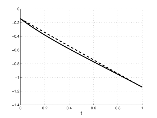
Consider the HRFMR with n=4𝑛4n=4. In this case, Re(λ2)=1Resubscript𝜆21\operatorname{Re}(\lambda_{2})=-1, so (23) becomes log(|x(t)c1n|)t+log(|x(0)c1n|)𝑥𝑡𝑐subscript1𝑛𝑡𝑥0𝑐subscript1𝑛\log(|x(t)-c1_{n}|)\approx-t+\log(|x(0)-c1_{n}|). Fig. 6 depicts log(|x(t)(1/4)14|)𝑥𝑡14subscript14\log(|x(t)-(1/4)1_{4}|) for the initial condition x(0)=[1000]𝑥0superscriptmatrix1000x(0)=\begin{bmatrix}1&0&0&0\end{bmatrix}^{\prime}. Note that here log(|x(0)(1/4)14|)=log(3/4)𝑥014subscript1434\log(|x(0)-(1/4)1_{4}|)=\log(\sqrt{3/4}). Also shown is the graph of t+log(3/4)𝑡34-t+\log(\sqrt{3/4}). It may be seen that the real convergence rate is slightly faster than the estimate in (23). \square

Refer to caption
Figure 6: log(|x(t)(1/4)14|)𝑥𝑡14subscript14\log(|x(t)-(1/4)1_{4}|) in the HRFMR with n=4𝑛4n=4 and x(0)=[1 0 0 0]𝑥0superscriptdelimited-[]1000x(0)=[1\;0\;0\;0]^{\prime} as a function of t𝑡t (solid line). Also shown is the function t+log(3/4)𝑡34-t+\log(\sqrt{3/4}) (dashed line).

IV An Application: orbital collective motion with limited communication

Consider a collection of n𝑛n agents moving along a circular ring of radius R𝑅R. The location of agent k𝑘k at time t𝑡t is

[Rcos(θk(t))Rsin(θk(t))],superscriptmatrix𝑅subscript𝜃𝑘𝑡𝑅subscript𝜃𝑘𝑡\begin{bmatrix}R\cos(\theta_{k}(t))&R\sin(\theta_{k}(t))\end{bmatrix}^{\prime}, (24)

and the dynamics is

θ˙k=uk,k=1,,n,formulae-sequencesubscript˙𝜃𝑘subscript𝑢𝑘𝑘1𝑛\dot{\theta}_{k}=u_{k},\quad k=1,\dots,n, (25)

i.e. uksubscript𝑢𝑘u_{k} controls the angular velocity of agent k𝑘k.

We say that the agents are in a balanced configuration at time t𝑡t if any two neighboring agents along the ring p,q𝑝𝑞p,q, with θp(t)θq(t)0subscript𝜃𝑝𝑡subscript𝜃𝑞𝑡0\theta_{p}(t)-\theta_{q}(t)\geq 0, satisfy θp(t)θq(t)=2π/nsubscript𝜃𝑝𝑡subscript𝜃𝑞𝑡2𝜋𝑛\theta_{p}(t)-\theta_{q}(t)={2\pi}/{n}. The goal is to design a control u=[u1,,un]𝑢superscriptmatrixsubscript𝑢1subscript𝑢𝑛u=\begin{bmatrix}u_{1},\dots,u_{n}\end{bmatrix}^{\prime} asymptotically driving the system to a balanced configuration. Furthermore, the control must be local in the sense that each uksubscript𝑢𝑘u_{k} should depend only on the state of agent k𝑘k and its neighbors. These type of problems arise in the formation control of unmanned autonomous systems (see, e.g., [25]).

In what follows we assume that the agents are numbered such that

0θ1(0)θ2(0)θn(0)<2π.0subscript𝜃10subscript𝜃20subscript𝜃𝑛02𝜋0\leq\theta_{1}(0)\leq\theta_{2}(0)\leq\dots\leq\theta_{n}(0)<2\pi. (26)
Proposition 3

Consider (25) with the nonlinear control

uk=(xk+11)xk,k=1,,n,formulae-sequencesubscript𝑢𝑘subscript𝑥𝑘11subscript𝑥𝑘𝑘1𝑛u_{k}=(x_{k+1}-1)x_{k},\quad k=1,\dots,n, (27)

where

x1subscript𝑥1\displaystyle x_{1} :=(θ1θn+2π)/(2π),assignabsentsubscript𝜃1subscript𝜃𝑛2𝜋2𝜋\displaystyle:=(\theta_{1}-\theta_{n}+2\pi)/(2\pi), (28)
xksubscript𝑥𝑘\displaystyle x_{k} :=(θkθk1)/(2π),k=2,,n.formulae-sequenceassignabsentsubscript𝜃𝑘subscript𝜃𝑘12𝜋𝑘2𝑛\displaystyle:=(\theta_{k}-\theta_{k-1})/(2\pi),\quad k=2,\dots,n.

Then

limt(θi(t)θi1(t))=2π/n,for all i.subscript𝑡subscript𝜃𝑖𝑡subscript𝜃𝑖1𝑡2𝜋𝑛for all 𝑖\lim_{t\to\infty}\left(\theta_{i}(t)-\theta_{i-1}(t)\right)=2\pi/n,\quad\text{for all }i. (29)

In other words, the system always converges to a balanced configuration. Note that (27) implies that uksubscript𝑢𝑘u_{k} only depends on θk1,θksubscript𝜃𝑘1subscript𝜃𝑘\theta_{k-1},\theta_{k}, and θk+1subscript𝜃𝑘1\theta_{k+1}. Thus, it can be implemented using local communication requirements.

Proof of Prop. 3. By (26), xk(0)[0,1]subscript𝑥𝑘001x_{k}(0)\in[0,1], k=1,,n𝑘1𝑛k=1,\dots,n, i.e. x(0)Cn𝑥0superscript𝐶𝑛x(0)\in C^{n}. Also,

2πx˙k2𝜋subscript˙𝑥𝑘\displaystyle 2\pi\dot{x}_{k} =θ˙kθ˙k1absentsubscript˙𝜃𝑘subscript˙𝜃𝑘1\displaystyle=\dot{\theta}_{k}-\dot{\theta}_{k-1}
=ukuk1absentsubscript𝑢𝑘subscript𝑢𝑘1\displaystyle=u_{k}-u_{k-1}
=xk1(1xk)xk(1xk+1).absentsubscript𝑥𝑘11subscript𝑥𝑘subscript𝑥𝑘1subscript𝑥𝑘1\displaystyle=x_{k-1}(1-x_{k})-x_{k}(1-x_{k+1}).

This means that the xisubscript𝑥𝑖x_{i}s follow the dynamics of the HRFMR with λc=12πsubscript𝜆𝑐12𝜋\lambda_{c}=\frac{1}{2\pi}. By Corollary 1, limtx(t)=Ave(x(0))1n=n11nsubscript𝑡𝑥𝑡Ave𝑥0subscript1𝑛superscript𝑛1subscript1𝑛\lim_{t\to\infty}x(t)=\operatorname{Ave}(x(0))1_{n}=n^{-1}1_{n}. Using (28) completes the proof. ∎

Note that since x(0)Cn𝑥0superscript𝐶𝑛x(0)\in C^{n}, x(t)Cn𝑥𝑡superscript𝐶𝑛x(t)\in C^{n} for all t0𝑡0t\geq 0. This means in particular that the angular distance between any two neighbors can never change sign, i.e., the dynamics leads to a balanced configuration without changing the relative order of the agents along the ring. Also, note that the term (xk+11)xksubscript𝑥𝑘11subscript𝑥𝑘(x_{k+1}-1)x_{k} in (27) is always non-positive.

Combining (25), (27) and Prop. 3 yields

limtθ˙k(t)subscript𝑡subscript˙𝜃𝑘𝑡\displaystyle\lim_{t\to\infty}\dot{\theta}_{k}(t) =limtuk(t)absentsubscript𝑡subscript𝑢𝑘𝑡\displaystyle=\lim_{t\to\infty}u_{k}(t)
=(n11)n1,for all k.absentsuperscript𝑛11superscript𝑛1for all 𝑘\displaystyle=(n^{-1}-1)n^{-1},\quad\text{for all }k.

If we change (27) to

uk=xk(xk+11)+v,k=1,,n,formulae-sequencesubscript𝑢𝑘subscript𝑥𝑘subscript𝑥𝑘11𝑣𝑘1𝑛u_{k}=x_{k}(x_{k+1}-1)+v,\quad k=1,\dots,n, (30)

with v𝑣v\in\mathbb{R}, then a similar analysis yields that the agents converge to a balanced configuration but now

limtθ˙k(t)subscript𝑡subscript˙𝜃𝑘𝑡\displaystyle\lim_{t\to\infty}\dot{\theta}_{k}(t) =(n11)n1+v,for all k.absentsuperscript𝑛11superscript𝑛1𝑣for all 𝑘\displaystyle=(n^{-1}-1)n^{-1}+v,\quad\text{for all }k.

Thus, the asymptotic common angular velocity can be shifted to any desired value. The price for that is that all agents must agree beforehand on the common value v𝑣v. In particular, taking v=(1n1)n1𝑣1superscript𝑛1superscript𝑛1v=(1-n^{-1})n^{-1} yields zero asymptotic angular velocity. Note that using this specific value only requires that each agent knows the total number of agents n𝑛n.

Example 9

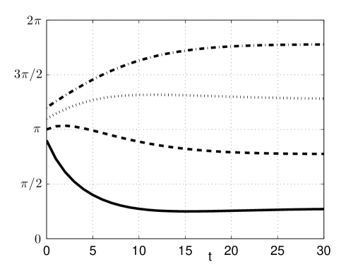
Consider the model (24), (25) with n=4𝑛4n=4, θ1(0)=0.9πsubscript𝜃100.9𝜋\theta_{1}(0)=0.9\piθ2(0)=πsubscript𝜃20𝜋\theta_{2}(0)=\pi, θ3(0)=1.1πsubscript𝜃301.1𝜋\theta_{3}(0)=1.1\pi and θ4(0)=1.2πsubscript𝜃401.2𝜋\theta_{4}(0)=1.2\pi. Fig. 7 depicts θ(t)𝜃𝑡\theta(t) for the control in (30) with v=(141)41=3/16𝑣1superscript41superscript41316v=(1-4^{-1})4^{-1}=3/16. It may be seen that θ(t)𝜃𝑡\theta(t) converges to θ¯:=[0.2768π0.7768π1.2768π1.7768π]assign¯𝜃superscriptmatrix0.2768𝜋0.7768𝜋1.2768𝜋1.7768𝜋\bar{\theta}:=\begin{bmatrix}0.2768\pi&0.7768\pi&1.2768\pi&1.7768\pi\end{bmatrix}^{\prime}, i.e., to a stationary configuration. Since θ¯iθ¯i1=0.5πsubscript¯𝜃𝑖subscript¯𝜃𝑖10.5𝜋\bar{\theta}_{i}-\bar{\theta}_{i-1}=0.5\pi for all i𝑖i, this configuration is also balanced. \square

Refer to caption
Figure 7: Dynamics of the model in Example 9: θ1(t)subscript𝜃1𝑡\theta_{1}(t) (solid line), θ2(t)subscript𝜃2𝑡\theta_{2}(t) (dashed), θ3(t)subscript𝜃3𝑡\theta_{3}(t) (dotted), and θ4(t)subscript𝜃4𝑡\theta_{4}(t) (dash-dot) as a function of t𝑡t.

V Discussion

Various models inspired by physics, such as the Vicsek et al. model [30] and Kuramoto oscillators, have played an important role in the development of consensus theory (see, e.g., [6, 3]).

The ribosome flow model on a ring (RFMR) is the mean field approximation of ASEP with periodic boundary conditions. In this paper, we reinterpreted the RFMR as a nonlinear consensus model. Indeed, the dynamics corresponds to a multi-agent system in which every agent interacts with its two closest neighbors on the ring only. Every solution converges to a stationary state and when all the transition rates are equal this stationary state corresponds to average consensus. A natural question for further research is what are the advantages of this nonlinear average consensus network with respect to the well-known linear average consensus network.

We analyzed the RFMR using tools from monotone dynamical systems theory. Our results show that the RFMR has several nice properties. It is an irreducible cooperative dynamical system admitting a continuum of linearly ordered equilibrium points, and every trajectory converges to an equilibrium point. The RFMR is on the “verge of contraction”, and it entrains to periodic transition rates.

Topics for further research include the following. ASEP with periodic boundary conditions has been studied extensively in the physics literature and many explicit results are known. For example, the time scale until the system relaxes to the (stochastic) steady state is known [1]. A natural research direction is based on extending such results to the RFMR.

For the RFM, that is, the mean-field approximation of ASEP with open boundary conditions, it has been shown that the steady-state translation rate R𝑅R satisfies the equation

0=f(R),0𝑓𝑅0=f(R),

where f𝑓f is a continued fraction in R𝑅R [14]. Using the well-known relationship between continued fractions and tridiagonal matrices (see, e.g., [32]) yields that R1/2superscript𝑅12R^{-1/2} is the Perron root of a certain non-negative symmetric tridiagonal matrix with entries that depend on the λisubscript𝜆𝑖\lambda_{i}[22]. This has many applications. For example it implies that R=R(λ0,,λn)𝑅𝑅subscript𝜆0subscript𝜆𝑛R=R(\lambda_{0},\dots,\lambda_{n}) in the RFM is a concave function on +n+1subscriptsuperscript𝑛1\mathbb{R}^{n+1}_{+} [22]. An interesting question is whether R𝑅R in the RFMR can also be described using such equations.

The irreducibility of the Jacobian J𝐽J plays a crucial role in the proof of global stability for monotone dynamical systems with a first integral [18, 17]. This seems reasonable, as convergence to consensus often requires some kind of connectivity in a corresponding communication graph [16]. An interesting research topic is the generalization of graph-theoretic conditions for convergence to consensus in time-varying linear consensus networks (see, e.g., [19]) to time-varying nonlinear monotone systems.

References

  • [1] R. A. Blythe and M. R. Evans, “Nonequilibrium steady states of matrix-product form: a solver’s guide,” J. Phys. A: Math. Theor., vol. 40, no. 46, pp. R333–R441, 2007.
  • [2] T. Chou, K. Mallick, and R. K. P. Zia, “Non-equilibrium statistical mechanics: from a paradigmatic model to biological transport,” Reports on Progress in Physics, vol. 74, p. 116601, 2011.
  • [3] F. Dorfler and F. Bullo, “Synchronization and transient stability in power networks and nonuniform Kuramoto oscillators,” SIAM J. Control Optim., vol. 50, no. 3, pp. 1616–1642, 2012.
  • [4] R. A. Horn and C. R. Johnson, Matrix Analysis, 2nd ed.   Cambridge University Press, 2013.
  • [5] Q. Hui and W. M. Haddad, “Distributed nonlinear control algorithms for network consensus,” Automatica, vol. 44, no. 9, pp. 2375–2381, 2008.
  • [6] A. Jadbabaie, J. Lin, and A. S. Morse, “Coordination of groups of mobile autonomous agents using nearest neighbour rules,” IEEE Trans. Automat. Control, vol. 48, pp. 988–1001, 2003.
  • [7] J. Ji-Fa, “Periodic monotone systems with an invariant function,” SIAM J. Math. Anal., vol. 27, pp. 1738–1744, 1996.
  • [8] P. D. Leenheer, D. Angeli, and E. D. Sontag, “Monotone chemical reaction networks,” J. Mathematical Chemistry, vol. 41, pp. 295–314, 2007.
  • [9] X. Liu, T. Chen, and W. Lu, “Consensus problem in directed networks of multi-agents via nonlinear protocols,” Physics Letters A, vol. 373, no. 35, pp. 3122–3127, 2009.
  • [10] W. Lohmiller and J.-J. E. Slotine, “On contraction analysis for non-linear systems,” Automatica, vol. 34, pp. 683–696, 1998.
  • [11] C. T. MacDonald, J. H. Gibbs, and A. C. Pipkin, “Kinetics of biopolymerization on nucleic acid templates,” Biopolymers, vol. 6, pp. 1–25, 1968.
  • [12] M. Margaliot, E. D. Sontag, and T. Tuller, “Entrainment to periodic initiation and transition rates in a computational model for gene translation,” PLoS ONE, vol. 9, no. 5, p. e96039, 2014.
  • [13] M. Margaliot and T. Tuller, “On the steady-state distribution in the homogeneous ribosome flow model,” IEEE/ACM Trans. Computational Biology and Bioinformatics, vol. 9, pp. 1724–1736, 2012.
  • [14] M. Margaliot and T. Tuller, “Stability analysis of the ribosome flow model,” IEEE/ACM Trans. Computational Biology and Bioinformatics, vol. 9, pp. 1545–1552, 2012.
  • [15] M. Margaliot and T. Tuller, “Ribosome flow model with positive feedback,” J. Royal Society Interface, vol. 10, p. 20130267, 2013.
  • [16] M. Mesbahi and M. Egerstedt, Graph Theoretic Methods in Multiagent Networks.   Princeton University Press, 2010.
  • [17] J. Mierczynski, “A class of strongly cooperative systems without compactness,” Colloq. Math., vol. 62, pp. 43–47, 1991.
  • [18] J. Mierczynski, “Cooperative irreducible systems of ordinary differential equations with first integral,” ArXiv e-prints, 2012. [Online]. Available: http://arxiv.org/abs/1208.4697
  • [19] L. Moreau, “Stability of multiagent systems with time-dependent communication links,” IEEE Trans. Automat. Control, vol. 50, pp. 169–182, 2005.
  • [20] R. Olfati-Saber, J. A. Fax, and R. M. Murray, “Consensus and cooperation in networked multi-agent systems,” Proc. IEEE, vol. 95, pp. 215–233, 2007.
  • [21] R. Olfati-Saber and R. M. Murray, “Consensus problems in networks of agents with switching topology and time-delays,” IEEE Trans. Automat. Control, vol. 49, pp. 1520–1533, 2004.
  • [22] G. Poker, Y. Zarai, M. Margaliot, and T. Tuller, “Maximizing protein translation rate in the ribosome flow model: the general case,” 2014, submitted.
  • [23] G. Russo, M. di Bernardo, and E. D. Sontag, “Global entrainment of transcriptional systems to periodic inputs,” PLOS Computational Biology, vol. 6, p. e1000739, 2010.
  • [24] A. Schadschneider, D. Chowdhury, and K. Nishinari, Stochastic Transport in Complex Systems: From Molecules to Vehicles.   Elsevier, 2011.
  • [25] R. Sepulchre, D. A. Paley, and N. E. Leonard, “Stabilization of planar collective motion with limited communication,” IEEE Trans. Automat. Control, vol. 53, pp. 706–719, 2008.
  • [26] H. L. Smith, Monotone Dynamical Systems: An Introduction to the Theory of Competitive and Cooperative Systems, ser. Mathematical Surveys and Monographs.   Providence, RI: Amer. Math. Soc., 1995, vol. 41.
  • [27] S. Srinivasa and M. Haenggi, “A statistical mechanics-based framework to analyze ad hoc networks with random access,” IEEE Trans. Mobile Computing, vol. 11, pp. 618–630, 2012.
  • [28] B. Tang, Y. Kuang, and H. Smith, “Strictly nonautonomous cooperative system with a first integral,” SIAM J. Math. Anal., vol. 24, pp. 1331–1339, 1993.
  • [29] G. Tripathy and M. Barma, “Driven lattice gases with quenched disorder: Exact results and different macroscopic regimes,” Phys. Rev. E, vol. 58, pp. 1911–1926, 1998.
  • [30] T. Vicsek, A. Czirok, E. Ben-Jacob, I. Cohen, and O. Shochet, “Novel type of phase transition in a system of self-driven particles,” Phys. Rev. Lett., vol. 75, pp. 1226–1229, 1995.
  • [31] M. Vidyasagar, Nonlinear Systems Analysis.   Englewood Cliffs, NJ: Prentice Hall, 1978.
  • [32] H. S. Wall, Analytic Theory of Continued Fractions.   Bronx, NY: Chelsea Publishing Company, 1973.
  • [33] Y. Zarai, M. Margaliot, and T. Tuller, “Explicit expression for the steady-state translation rate in the infinite-dimensional homogeneous ribosome flow model,” IEEE/ACM Trans. Computational Biology and Bioinformatics, vol. 10, pp. 1322–1328, 2013.
  • [34] Y. Zarai, M. Margaliot, and T. Tuller, “Maximizing protein translation rate in the ribosome flow model: the homogeneous case,” IEEE/ACM Trans. Computational Biology and Bioinformatics, 2014, to appear.
  • [35] R. Zia, J. Dong, and B. Schmittmann, “Modeling translation in protein synthesis with TASEP: A tutorial and recent developments,” J. Statistical Physics, vol. 144, pp. 405–428, 2011.