Using the Quantum Zeno Effect for Suppression of Decoherence

Abstract

Projective measurements are an essential element of quantum mechanics. In most cases, they cause an irreversible change of the quantum system on which they act. However, measurements can also be used to stabilize quantum states from decay processes, which is known as the Quantum Zeno Effect (QZE). Here, we demonstrate this effect for the case of a superposition state of a nuclear spin qubit, using an ancilla to perform the measurement. As a result, the quantum state of the qubit is protected against dephasing without relying on an ensemble nature of NMR experiments. We also propose a scheme to protect an arbitrary state by using QZE.

• August 2015

Keywords: Quantum Zeno Effect, Decoherence Suppression, NMR

1 Introduction

Interactions between a quantum system and its environment lead to changes of the system state and can result in the loss of coherence. This effect, often called decoherence, is a limiting factor for many applications, such as quantum computing. The loss of information associated with this process can be measured by the decreasing overlap between the initial and current states. This overlap (state fidelity) changes quadratically for times short enough compared to the inverse of the strength of the system-environment coupling and the correlation time of the environment, provided this coupling is also static on the relevant timescale [1, 2]. If such a system is repeatedly projected back to the original state by measurements performed before the state has changed significantly, the effect of the system-environment interaction can be effectively eliminated in the limit of sufficiently frequent measurements. This is termed the Quantum Zeno Effect (QZE) [3]. There are many potential applications of QZE, like entanglement generation [4], quantum metrology [5, 6], and quantum imaging [7].

It is worth mentioning that QZE is different from dynamical decoupling, which also suppresses decoherence. Although both schemes were unified from the viewpoint of a strong interaction between a system of interest and the others [8], there is a clear difference between them. While dynamical decoupling uses unitary control to average out the system-environment interaction [9], the non-unitary dynamics introduced by the measurements is essential for the state stabilization in QZE.

In the simplest case, the evolution suppressed by QZE is driven by a single interaction to a static external degree of freedom. Typical examples include a transition between two states of a single trapped ion [10], nuclear magnetic resonance (NMR) [11], and atomic systems [12, 13]. Another example is the confinement of a unitary dynamics in a specific subspace, as demonstrated in a rubidium Bose Einstein condensate [14]. In a more sophisticated case, QZE restrains the non-unitary dynamics of an open quantum system [3], instead of suppressing a unitary evolution driven by external fields. One experiment controlled such non-unitary dynamics, the escape rate of atoms from a trap, using the QZE [15]. However, QZE to suppress the dephasing of a two-level system was not demonstrated yet.

In this paper, we present a proof-of-principle demonstration that QZE is equally possible to stabilize the state of a quantum system subject to dephasing by successive measurements. We employ a liquid-state NMR Quantum Computer with a two-spin molecule. However, the ensemble nature of NMR is not essential to implement the measurements in our experiments, unlike in [11, 16]. A similar scheme was proposed for a non-ensemble system in [17]. Also, QZE experiments without relying on an ensemble average were reported [18].

This paper is organized as follows. In Sec. II, a brief review on QZE and a detailed theoretical background of our experiment are presented. We show a proof-of-principle demonstration, including a characterization of the molecule employed in our experiments, in Sec. III. The last section is devoted to conclusion and discussions, where we propose a scheme to protect an arbitrary state by using QZE.

2 Theory

2.1 Quantum Zeno Effect

In order to understand the essence of QZE, it is sufficient to consider a coherent superposition of a qubit being dephased by a randomly fluctuating classical field [1, 2], with the concept of “mixing process” [19]. The relevant Hamiltonian is thus

$$\mathcal{H}(t) = H_{s}+H_{I}+H_{en},$$ (1)

$$H_{s} = \frac{\omega_{s}}{2}\sigma_{z},$$ (2)

$$H_{I} = \lambda\sigma_{z}\hat{A},$$ (3)

$$H_{en} = \omega_{en}\hat{B},$$ (4)

where $\omega_{s}$ denotes the energy of the system, $\lambda$ denotes the strength of the fluctuating field, $\hat{A}$ denotes the environmental operator to represent the interaction with the system, $\omega_{en}$ denotes the environmental energy, $\hat{B}$ denotes the environmental operator, and $\sigma_{i}$ is a Pauli matrix. The Hamiltonian contains only $\sigma_{z}$ because only pure dephasing is considered. We go to an interaction picture, obtaining

$$H_{I}(t)\simeq\lambda\sigma_{z}\hat{A}(t),$$ (5)

where $\hat{A}(t)=e^{i\omega_{en}\hat{B}}\hat{A}e^{-i\omega_{en}\hat{B}}$.

We prepare a superposition state $\displaystyle|+\rangle=\frac{1}{\sqrt{2}}(|0\rangle+|1\rangle)$ for the system. The density matrix of the system and the environment is $\displaystyle\rho(0)=\rho_{s}(0)\otimes\rho_{en}$ where $\rho_{s}(0)=|+\rangle\langle+|$ and $\rho_{en}$ denotes the initial state of the environment. Formally integrating the von Neumann equation $\dot{\rho}=-i[\mathcal{H},\rho]$, we obtain

$$\rho(t)=\rho(0)-i\lambda\int_{0}^{t}dt_{1}[\sigma_{z}\hat{A}(t_{1}),\rho(t_{1})].$$

The natural unit system with $\hbar=1$ is used. Iterating $\rho(t_{1})$ on the right hand side and replacing $\rho(t_{2})$ by $\rho(0)$, we have the second order expression

$$\rho(t) \simeq \rho(0)-i\lambda\int_{0}^{t}dt_{1}[\sigma_{z}\hat{A}(t_{1}),\rho(0)]$$

$$- \lambda^{2}\int_{0}^{t}\int_{0}^{t_{1}}dt_{1}dt_{2}[\sigma_{z}\hat{A}(t_{1}),[\sigma_{z}\hat{A}(t_{2}),\rho(0)]].$$

Tracing out the environment, we get

$$\rho_{s}(t) = \rho_{s}(0)-\lambda^{2}\int_{0}^{t}\int_{0}^{t_{1}}dt_{1}dt_{2}\langle\hat{A}(t_{1})\hat{A}(t_{2})\rangle[\sigma_{z},[\sigma_{z},\rho_{s}(0)]].$$ (6)

where $\rho_{s}(t)={\rm Tr}_{en}[\rho(t)]$ denotes the density operator of the system, ${\rm Tr}_{en}[\cdots]$ denotes a partial trace of the environment, and $\langle\hat{A}(t_{1})\hat{A}(t_{2})\rangle={\rm Tr}[\hat{A}(t_{1})\hat{A}(t_{2})\rho_{en}]$ denotes a correlation function. Here, we assume an unbiased noise $\langle\hat{A}(t)\rangle={\rm Tr}[\hat{A}(t)\rho_{en}]\simeq 0$ and a time symmetry $\langle\hat{A}(t_{1})\hat{A}(t_{2})\rangle=\langle\hat{A}(t_{2})\hat{A}(t_{1})\rangle$.

If the correlation time of the noise is much shorter than the relevant time scale of the system [20], the duration of each measurement in our case, we can approximate the correlation function by a $\delta$-function

$$\langle\hat{A}(t_{1})\hat{A}(t_{2})\rangle=2\tau_{c}\delta(t_{1}-t_{2}),$$

where $\tau_{c}$ is the correlation time. Substituting into Eq. (6), we have $\rho_{s}(t)\simeq\rho_{s}(0)-\lambda^{2}\tau_{c}t[\sigma_{z},[\sigma_{z},\rho_{s}(0)]].$ The state fidelity $F(t)=\langle+|\rho_{s}(t)|+\rangle$ is then

$$F(t)\simeq 1-2\lambda^{2}\tau_{c}t,$$ (7)

which corresponds to a linear decay. It is a well known fact QZE is not observable in this regime [3].

In the opposite limit of a slowly fluctuating environment, where $|t_{1}-t_{2}|\ll\tau_{c}$, the correlation function is constant,

$$\langle\hat{A}(t_{1})\hat{A}(t_{2})\rangle=1,$$

and Eq. (6) becomes $\rho_{s}(t)\simeq\rho_{s}(0)-\frac{1}{2}\lambda^{2}t^{2}[\sigma_{z},[\sigma_{z},\rho_{s}(0)]]$ for $\lambda^{2}\tau_{c}t$ $\ll$ $1$, i.e., the decoherence quadratically starts:

$$F(t)\simeq 1-\lambda^{2}t^{2}.$$ (8)

This is the regime the QZE can be observed: if $N$ sequential projective measurements of $|+\rangle\langle+|$ are carried out on the system and the delay between the measurements is short compared to the correlation time, $T/N\ll\tau_{c}$, the system remains in the initial state with a probability $P(N)=(F(T/N))^{N})\simeq\left(1-\frac{\lambda^{2}T^{2}}{N^{2}}\right)^{N}\simeq e^{-\frac{\lambda^{2}T^{2}}{N}}$ . Since the exponent can become arbitrarily small for large $N$, the decoherence vanishes asymptotically.

2.2 Theoretical Background of Experiment

We intend to show a proof-of-principle demonstration with NMR that QZE is employed for protecting a phase decoherence. We need to answer two questions: 1) how to obtain a system that shows a quadratic decay. 2) how to measure a quantum system without employing ensemble averages, unlike usual NMR experiments [11, 16].

2.2.1 Quadratic Decay.

A molecule in a solvent strongly and rapidly interacts with molecules of the solvent. These interactions are so strong and rapid that they effectively cancel with each other. Therefore, the effective interaction between the molecule and the solvent is often small [21]. This phenomenon is called motional narrowing. Since $T_{1}$ and $T_{2}$ of a spin in the molecule become longer, peaks in its NMR spectrum become sharper. The total number of quantum gates that can be performed within the coherence time is estimated as $T_{2}/\tau_{G}$, where $\tau_{G}$ denotes the time of the gate operation. These long $T_{2}$ guarantees many quantum operations and liquid state NMR is often employed to demonstrate quantum algorithms.

We introduce molecules with magnetic dipole moments, originated from electrons, into the solvent. These molecules generate strong but short range magnetic fields. They are short range in the sense that they decay with $r^{-3}$ or faster as a function of $r$, the distance. These molecules are called magnetic impurities. They also move rapidly in the solvent. When a magnetic impurity passes by a molecule, a strong interaction between a spin in the molecule and the magnetic impurity changes the spin state abruptly. Such an interaction leads to a final spin state uncorrelated to the initial one. Motional narrowing does not occur, since there are not enough magnetic impurities for their effects to be canceled on average.

The interaction of the spin with the magnetic impurity is a $\delta$ function-like in time, and thus we do not expect a quadratic decay of the spin state. The higher density of the magnetic impurity leads to shorter $T_{1}$ and $T_{2}$, but the characteristic of the state decay is always linear, like in Eq. (7).

Now, let us consider a two-spin molecule. One of the two spins (called E) is under the influence of a magnetic impurity and interacts with the other spin (called S) through a scalar coupling (for simplicity, the weak coupling limit [22] is assumed)

$$\mathcal{H}_{\rm J}=J\sigma_{z}^{\rm S}\sigma_{z}^{\rm E}/4,$$ (9)

where $\sigma_{i}^{\rm E}$ $(\sigma_{i}^{\rm S})$ is a Pauli operator acting on the spin E (S). $J$ is the strength of the scalar coupling, in frequency units. The spin S interacts only with the spin E and free from the magnetic impurity. The delta function-like interaction on the spin E due to the magnetic impurity is transformed into a slower interaction on the spin S by the scalar coupling. In this case, $J$ and $T_{1}$ of the spin E determine the correlation time. However, for the case considered in this paper, the $J$ term is more essential in the practical range of $T_{1}$ of the spin E and the correlation time becomes of the order of $2\pi/J$.

We can obtain a spin showing a quadratic decay with a two-spin molecule and magnetic impurities. The correlation time is of the order of $2\pi/J$, usually of few milliseconds for a carbon and hydrogen nuclei combination and thus this interaction is well controllable with NMR techniques. A similar approach has been reported, but using a series of pulses instead of magnetic impurities [19].

2.2.2 Projective Measurements.

A field gradient was often employed as a projective measurement in NMR experiments [11, 16]. However, it is based on a spacial averaging, or the ensemble nature of NMR, and thus it is considered as a mere simulation of a projective measurement. Therefore, we cannot employ a field gradient as a projective measurement in our experiment.

We have to implement a measurement according to its definition. A measurement of a system means the system is entangled to a measurement apparatus. Then, the measurement apparatus falls into one of its eigenstates. The corresponding eigenvalue is treated as the measured value [23]. According to this idea, we are able to implement a non-selective measurement $M_{\rm DS}$ with another qubit, called a device (D), as follows

$$M_{\rm DS}(\rho) = \frac{1}{2}Ad({\mathcal{E}}_{1},\rho)+\frac{1}{2}Ad({\mathcal{E}}_{2},\rho),$$ (10)

where $Ad(*,\rho)=*\rho*^{\dagger}$, ${\mathcal{E}}_{1}=CNOT_{\rm DS}$ and ${\mathcal{E}}_{2}=\sigma_{y}^{\rm D}\,CNOT_{\rm DS}$. $CNOT_{\rm DS}$ is a CNOT gate whose control and target qubits are the device D and the system S, respectively. We employ $CNOT_{\rm DS}$ as an entangler, while $\sigma_{y}^{\rm D}$ causes the phase decoherence of the device D [24]. This measurement operation is virtual and instantaneous. This procedure is effective when the system and device are not correlated before the measurements are performed. Such condition is satisfied, since the device is perfectly decohered by the operator $\sigma_{y}^{D}$ at the end of each measurement.

It is worth mentioning that we use a stochastic master equation to describe the measurement, and such a master equation usually requires an average of the measurement outcomes [20]. However, the average technique is not against the fact that our scheme does not rely on the nature of ensemble average. Even for a single spin, one needs to repeat the experiment many times, and needs to take an average of the measurement results. For example, in [25], they consider a single NV center, and a model similar to ours is applied to include the fluctuating noise, using an average. Similarly, our calculation described here can be applied to a single spin.

2.2.3 QZE Simulation.

We combine the ideas in § 2.2.1 and § 2.2.2 to design an ideal QZE simulation. We consider a three-qubit system. The first qubit is a system S of which phase is protected. The second qubit E mediates and filters the random noise caused by a magnetic impurity to the system. The third qubit is a device D.

First, we consider a time development without $M_{\rm DS}$ as follows.

$$\left[\tau_{xy}\right]^{N},$$ (11)

where $\tau_{xy}$ is the period when the system decoheres and $N$ is the number of repetitions. We describe the open system dynamics with the operator sum formalism [26]. The density matrix change during $\tau_{xy}$ is

$$\rho\rightarrow(1-p_{e}\tau_{xy})Ad(e^{-i{\mathcal{H}}_{\rm J}\tau_{xy}},\rho)+p_{e}\tau_{xy}Ad\left((\sigma_{x}^{\rm E}\cos\theta+\sigma_{y}^{\rm E}\sin\theta)e^{-i{\mathcal{H}}_{\rm J}\tau_{xy}},\rho\right),$$ (12)

where $p_{e}$ determines the strength of decoherence, $\sigma_{i}^{\rm E}$ is a $\sigma_{i}$ operator acting on the spin E, and $\theta$ is a random variable indicating the rotation axis of the $\pi$-rotation on the spin E, caused by the magnetic impurity. $p_{e}$ is a function of the concentrations of the magnetic impurity and the molecule of interest. Since the initial state of E is $|0\rangle\langle 0|_{E}$ and $H_{J}$ contains only $\sigma_{z}^{\rm E}$, $Ad((\sigma_{x}^{\rm E}\cos\theta+\sigma_{y}^{\rm E}\sin\theta)^{n},|0\rangle\langle 0|_{E})$ is equivalent to $Ad((\sigma_{y}^{\rm E})^{n},|0\rangle\langle 0|_{E})$ for the interaction $H_{J}$, where $n$ is an arbitrary integer. Therefore, we can replace the second term of $\sigma_{x}^{\rm E}\cos\theta+\sigma_{y}^{\rm E}\sin\theta$ by $\sigma_{y}^{\rm E}$. We show the simulation results (red and green) with $p_{e}=0.05$ and $0.00$ in figure 1. The initial state is $|+\rangle\langle+|_{S}\otimes|0\rangle\langle 0|_{E}\otimes|0\rangle\langle 0|_{D}$. figure 2 shows the differences between simulations of $p_{e}=0.05$ (red) and $0.00$ (green) in the initial stage of the dynamics, shown in figure 1. A quadratic behaviour is observed.

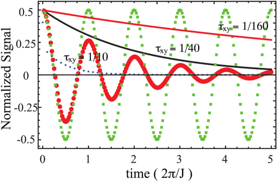
Figure 1: Simulated FID signal with $p_{e}=0.05$ by Eq. (11) (large red) that shows oscillatory behaviour but decays in time. The data without decay (green) is the case of $p_{e}=0$ and is shown for comparison. The three curves without oscillatory behaviours are simulations with the measurement $M_{\rm DS}$. The red curve with $\displaystyle\tau_{xy}=1/160$ decays slower than the black one, with $\displaystyle\tau_{xy}=1/40$, as expected. The blue curve (dots) with $\displaystyle\tau_{xy}=1/10$ decays even faster than the envelope of the simulated FID signal.

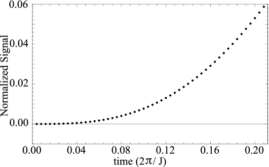
Figure 2: The differences between simulations with $p_{e}=0.05$ (red) and $0.00$ (green) in the initial stage of the dynamics, shown in figure 1. A quadratic behaviour is observed.

Second, we introduce $M_{\rm DS}$ as follows.

$$\left[\tau_{xy}-M_{\rm DS}\right]^{N}$$ (13)

We show the simulation results with $p_{e}=0.05$ and three different $\tau_{xy}$’s in figure 1. The result with $\displaystyle\tau_{xy}=1/40$ (black) decays faster than that of $\displaystyle\tau_{xy}=1/160$ (red), as expected. The result with $\displaystyle\tau_{xy}=1/10$ decays even faster than the envelope of the simulated FID.

We can obtain the same results of figure 1 with $M_{ES}$, where $E$ is the spin mediating the random noise. $M_{\rm ES}$ is obtained replacing $CNOT_{\rm DS}$ and $\sigma_{y}^{\rm D}$ (equivalent with $\sigma_{x}^{\rm D}\cos\theta+\sigma_{y}^{\rm D}\sin\theta$) in Eq. (10) with $CNOT_{\rm ES}$ and $\sigma_{x}^{\rm E}\cos\theta+\sigma_{y}^{\rm E}\sin\theta$ (equivalent with $\sigma_{y}^{\rm E}$), respectively. It implies that we are able to measure the system S with the spin E, without introducing the device (third spin) D.

3 Experiments and Simulations

3.1 Sample

Our spectrometer is a JEOL ECA-500. The experiments were carried out using a ¹³C-labeled chloroform (Cambridge Isotopes) diluted in $d_{6}$-acetone with a 303 mM concentration, at room temperature. We added a magnetic impurity (47.7 mM of Iron(III) acetylacetonate, a relaxation agent to control $T_{1}$ and $T_{2}$ in NMR experiments) to the solution, which mainly introduces a random flip-flop motion of the ¹H spin, since the carbon atom is surrounded and protected by three chlorine and one ¹H atoms, as illustrated in the inset of figure 3. This is a realization of the configuration discussed in § 2.2.1.

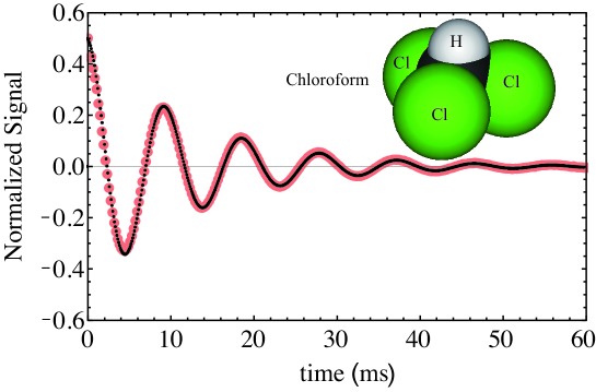
Figure 3: Measured (large red) and simulated (small black) FID signals of ¹³C. The ¹³C atom is in the center of the schematic chloroform molecule, surrounded by the ¹H and the three chlorine atoms. The selected parameters are $(T_{d},1/p_{s})=(6.5,300)$ ms. $T/N_{t}=0.1$ ms in Eq. (17) is taken for the computation.

3.1.1 $T_{1}$ and $T_{2}$ Measurements and Bang-Bang Control

To characterize the sample, we measured $T_{1}$ and $T_{2}$ of the ¹H and ¹³C spins. $T_{1}$ and $T_{2}$ of the ¹H are both about 7 ms. It is reasonable because the magnetic impurity simultaneously flips spins and destroys their phase coherence. On the other hand, $T_{1}$ of the ¹³C spin is 300 ms, while its $T_{2}$ is 17 ms. Without the magnetic impurities, $T_{1}$ and $T_{2}$ of the ¹³C spin are 20 s and 0.3 s [27]. So, the $T_{2}$ relaxation is speed up by about 20 times. We measured $T_{1}$ using the standard inversion recovery sequence. Due to a good field homogeneity, $T_{2}$ can be obtained directly from the Free Induction Decay (FID) signal [22], see figure 3. This shorter $T_{2}$, compared with $T_{1}$, can be understood according to the discussion in § 2.2.1. For our sample, $J/2\pi\approx 215$ Hz.

We expect a quadratic decay in the FID signal as shown in figure 2. It is, however, difficult to observe such behaviour due to experimental limitations. Therefore, we performed Bang-Bang controls on our sample, as shown in figure 4. Bang-Bang controls also require a quadratic decay to be effective and thus we are able to judge if our sample have it at the initial stage of decoherence. The effective $T_{2}$ of the ¹³C is measured through the application of a XY-4 sequence [28, 29], which compensates pulse imperfections, to the ¹³C spin. When the interval between the pulses is below 4 ms, the effective $T_{2}$ becomes longer. We observe a maximum in figure 4 which may be understood by the discussions in [30, 31]. We will consider this elsewhere.

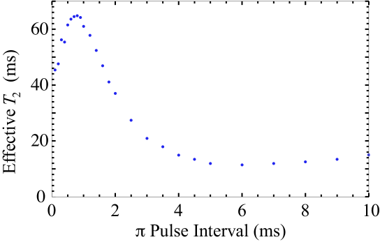
Figure 4: Effective $T_{2}$’s of the ¹³C spin as a function of the intervals between $\pi$-pulses of the XY-4 sequence applied to the ¹³C spin.

Further, we also measured this effective $T_{2}$ applying a series of $\pi$-pulses to the ¹H spin, as shown in figure 5. If they are frequent enough, these $\pi$-pulses effectively decouple the ¹H and the ¹³C spins, as well known in NMR [22]. The effective $T_{2}$ at the $\pi$-pulse interval of 0.2 ms becomes $97/17\sim 6$ times longer than that without $\pi$-pulses. This result indicates that the dominant (more than 80 %) source of the decoherence of the ¹³C spin is the ¹H one.

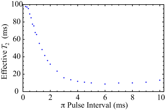
Figure 5: Effective $T_{2}$’s of the ¹³C spin as a function of the intervals between $\pi$-pulses of the XY-4 sequence applied to the ¹H spin.

3.1.2 Simulation of the FID with operator sum formalism.

We reproduce the observed FID signal shown in figure 3 using the operator sum formalism [26].

The thermal state density matrix of the two qubit system is well approximated as

$$\rho=\left(\frac{\sigma_{0}}{2}\right)^{\otimes 2}+\epsilon_{s}\frac{\sigma_{z}\otimes\sigma_{0}}{4}+\epsilon_{e}\frac{\sigma_{0}\otimes\sigma_{z}}{4},$$ (14)

where $\epsilon_{i}=\hbar\omega_{i}/2k_{B}T$, $\omega_{i}$ is the Larmor frequency of the $i$-th spin, and $\sigma_{0}$ is the identity matrix of dimension 2. The suffixes $s$ and $e$ denote the ¹³C and ¹H spin, respectively. Eq. (14) can be rewritten as

$$\rho=(1-\epsilon_{s})\left(\frac{\sigma_{0}}{2}\right)^{\otimes 2}+\epsilon_{s}|0\rangle\langle 0|\otimes\frac{\sigma_{0}}{2}+\epsilon_{e}\frac{\sigma_{0}\otimes\sigma_{z}}{4}.$$

Since the trace of the NMR observable, such as $\sigma_{x,y}$, is zero, the term $(1-\epsilon_{s})\left(\sigma_{0}/2\right)^{\otimes 2}$ cannot be observed in NMR experiments and can be ignored. Moreover, only the ¹³C spin is observed (or, $Tr\left(\sigma_{x,y}\otimes\sigma_{0},\rho\right)$ is measured), the above density matrix can be regarded as $\epsilon_{s}\rho_{\rm th}$, where $\rho_{\rm th}=|0\rangle\langle 0|\otimes(\sigma_{0}/2)$. This state can be normalized as a pseudopure state $|0\rangle\langle 0|$ for the ¹³C spin, without any initialization operation.

The effect of the ¹H spin in the ¹³C spin dynamics during the FID can be explained with Eq. (12) taking the ¹H spin as the spin E. $p_{e}$ is given as $1/(2T_{d})$ where $T_{d}$ is the flip-flopping time constant. When the evolution time $T$ is divided into $N_{t}$ equal steps, the state after the $i$-th step is obtained as

$$\rho_{i+1} = \left(1-p_{e}\frac{T}{N_{t}}\right)Ad(e^{-i{\mathcal{H}}_{J}T/N_{t}},\rho_{i})+p_{e}\frac{T}{N_{t}}Ad\left(\left(\sigma_{0}\otimes\sigma_{y}\right)e^{-i{\mathcal{H}}_{J}T/N_{t}},\rho_{i}\right).$$ (15)

In our experiments, we also have to take into account a longitudinal relaxation of the ¹³C spin, a process towards the thermal state, which is $\rho_{th}$ in our case [24]. It can be described as

$$\rho_{i+1}=\left(1-p_{s}\frac{T}{N_{t}}\right)Ad(e^{-i{\mathcal{H}}_{J}T/N_{t}},\rho_{i})+p_{s}\frac{T}{N_{t}}\rho_{\rm th},$$ (16)

where $p_{s}$ is expected to be the inverse of $T_{1}$ of the ¹³C spin.

When the dynamics of both the ¹³C and ¹H spins are considered, the state after the $i$-th iteration is

$$\ \rho_{i+1} = \left(1-\left(p_{s}+p_{e}\right)\frac{T}{N_{t}}\right)Ad(e^{-i{\mathcal{H}}_{J}T/N_{t}},\rho_{i})+p_{e}\frac{T}{N_{t}}Ad(\sigma_{0}\otimes\sigma_{y},\rho_{i})+p_{s}\frac{T}{N_{t}}\rho_{\rm th},$$ (17)

where $\left(\sigma_{0}\otimes\sigma_{y}\right)e^{-i{\mathcal{H}}_{J}T/N_{t}}$ is approximated as $\sigma_{0}\otimes\sigma_{y}$. This approximation is valid because we take $N_{t}$ such that $JT/N_{t}\ll 1$.

Black small dots in figure 3 show the simulated FID signal with $T/N_{t}=0.1$ ms. Taking a proper parameter set of $(T_{d},1/p_{s})=(6.5,300)$ ms, our simulation reproduces the measured FID signal very well. $T_{d}$ and $1/p_{s}$ are equal to $T_{2}(=T_{1})$ of the ¹H spin and $T_{1}$ of the ¹³C spin within experimental errors, respectively.

3.2 QZE Experiments

We take the ¹³C and ¹H spins as S and E in § 2.2.3, respectively. We do not require a readout of the measurements, and thus a non-selective measurement is sufficient to observe the QZE. The initial state for our experiments is $|+\rangle\langle+|\otimes\sigma_{0}/2=Ad\left(e^{-i\frac{\pi}{2}\sigma_{y}/2}\otimes\sigma_{0},\rho_{\rm th}\right)$, obtained applying a $\pi/2$ pulse to the thermal state $\rho_{\rm th}$.

3.2.1 Implementation of Non-Selective Measurements.

The essential role of the $CNOT$s in $M_{\rm ES}$ and $M_{\rm DS}$ in § 2.2 is to entangle the two spins. So, we are able to employ another entangler, $e^{-i\pi\sigma_{z}\otimes\sigma_{z}/4}$ [32], which is locally equivalent to the CNOT employed in $M_{ES}$. Our measurement procedure is as follows,

1. applying $\displaystyle e^{\pm i\frac{\pi}{2}\sigma_{y}/2}\otimes\sigma_{0}$

2. a time delay $\tau_{z}$

3. applying $\displaystyle e^{\mp i\frac{\pi}{2}\sigma_{y}/2}\otimes\sigma_{0}$

and we call this sequence $M_{\pm}(\tau_{z})$ [32]. The first and third steps can be almost ideally implemented with composite pulses (SCROFULOUS [33]). During the second step, the ¹³C and ¹H spins are entangled via ${\mathcal{H}}_{J}$ and the ¹H spin decoheres simultaneously. The dynamics of the ¹³C spin due to $M_{\pm}(\tau_{z})$ is non-unitary, in contrast to the unitary control used in dynamical decoupling sequences. If we ignore the relaxation in the step (ii), $M_{\pm}(\tau_{z})$ is equivalent to

$$\left(e^{\mp i\frac{\pi}{2}\sigma_{y}/2}\otimes\sigma_{0}\right)e^{-i(J\tau_{z})\sigma_{z}\otimes\sigma_{z}/4}\left(e^{\pm i\frac{\pi}{2}\sigma_{y}/2}\otimes\sigma_{0}\right)=e^{\mp i(J\tau_{z})\sigma_{x}\otimes\sigma_{z}/4}.$$ (18)

This operator entangles the spins.

We need to optimize the $\tau_{z}$ value in our experiments, since it should satisfy some conflicting conditions. To maximally entangle the spins, we should have $\tau_{z}=\frac{2\pi}{2J}\approx 2.5$ ms. To fully decohere the ¹H spin, we should have $\tau_{z}$ longer than $T_{2}$ for the proton spin. However, a longer $\tau_{z}$ reduces the QZE due to ¹³C longitudinal relaxation.

To perform the QZE experiment, we employ the pulse sequence

$$\left[\tau_{xy}~{}-~{}M_{\pm}(\tau_{z})\right]^{N},$$ (19)

where $\tau_{xy}$ indicates a waiting time when the phase decoherence occurs. We replace $M_{\rm DS}$ in Eq. (13) with a realistic $M_{\pm}(\tau_{z})$, which is equally effective as a measurement.

We confirm the importance of the period $\tau_{z}$ in our measurement ($M_{\pm}(\tau_{z})$) taking $\tau_{z}=0$ in figure 6. It is easy to see that $M_{\pm}(0)$ is an identity operator from Eq. (18). Therefore, we expect that an experiment of $[\tau_{xy}-M_{\pm}(0)]^{N}$ reproduces the FID signal shown in figure 3, if we take into account of $\tau_{M}$ (the period of $M_{\pm}(0)$ = two successive composite pulses). The results with $\tau_{xy}=0.3,0.5,1.0$ and 1.5 ms are identical with the FID signal. The results with $\tau_{xy}=$ 0.1 and 0.2 ms are distorted, which may be caused by the fact that our spectrometer cannot produce such frequent pulses. The results described in figure 6 demonstrate that the composite $\frac{\pi}{2}$ pulses do not change the decay dynamics induced by the proton spin, as long as no entangler is applied.

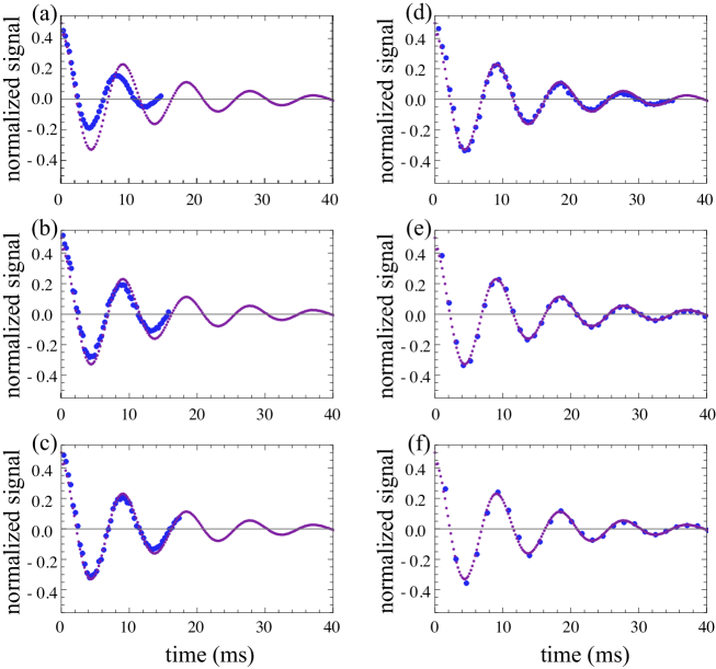
Figure 6: QZE experiments with $M_{-}(0)$ when $\tau_{xy}=$ (a) 0.1, (b) 0.2, (c) 0.3, (d) 0.5, (e) 1.0, and (f) 1.5 ms. The $x$-coordinate of the $n$’th point is calculated with $n(\tau_{M}\alpha+\tau_{xy})$, where $\alpha$ is a fitting parameter. $\tau_{M}=2\times 58~{}\mu$s is the period of two successive composite pulses, while we choose $\alpha=0.4$ for these experiments to reproduce the FID signal best. They are compared with the measured FID signal (small red points).

3.2.2 QZE Experiments and Simulations.

The simulation of the dynamics of the ¹³C spin during the QZE experiment is performed as follows. The pulse sequence of Eq. (19) is divided into

$$[\tau_{xy}-e^{\pm i\frac{\pi}{2}\sigma_{y}/2}\otimes\sigma_{0}-\tau_{z}-e^{\mp i\frac{\pi}{2}\sigma_{y}/2}\otimes\sigma_{0}]^{N},$$

where $e^{\pm i\frac{\pi}{2}\sigma_{y}/2}\otimes\sigma_{0}$ is a composite $\pi/2$ pulse acting on the ¹³C spin in the step (i) or (iii) in $M_{\pm}(\tau_{z})$. The time developments during both $\tau_{xy}$ and $\tau_{z}$ are calculated using the Eq. (17). Additionally, the time development $(\rho\rightarrow\rho^{\prime})$ during the composite $\pi/2$-pulse with the duration $\tau=58~{}\mu$s is calculated by

$$\rho^{\prime} = \left(1-\left(p_{s}+p_{e}\right)\tau\right)Ad(e^{-i(\mp\frac{\pi}{2}\frac{\sigma_{y}}{2}\otimes\sigma_{0}+{\mathcal{H}}_{J}\tau)},\rho)+p_{e}\tau Ad(\sigma_{0}\otimes\sigma_{y},\rho)+p_{s}\tau\rho_{\rm th}.$$ (20)

For example, in the case of $\tau_{xy}=0.3$ ms and $\tau_{z}=2.0$ ms, a detailed simulation procedure is as follows. The initial state of the experiment is $|+\rangle\langle+|\otimes\sigma_{0}$, which can be obtained after the application of a $\pi/2$ pulse to $\rho_{th}$. The output of each step is the input of the next one.

a:

Simulating the time development during $\tau_{xy}$ with Eq. (17). We iterate this 3 times because $\tau_{xy}=0.3$ ms and $T/N_{t}=0.1$ ms.

b:

The evolution of the state during the first rotation, $e^{\pm i\frac{\pi}{2}\sigma_{y}/2}\otimes\sigma_{0}$, is calculated using the Eq. (20).

c:

The time development during $\tau_{z}$ is simulated with Eq. (17). Since $\tau_{z}=2$ ms, this is iterated 20 times.

d:

The effects of the second rotation, $e^{\mp i\frac{\pi}{2}\sigma_{y}/2}\otimes\sigma_{0}$, are taken into account using Eq. (20).

After this last step, the whole procedure is repeated $N$ times.

Figure 7 shows the results of the QZE experiments with $M_{-}(\tau_{z})$ varying the parameter $\tau_{xy}$, but keeping a constant $\tau_{z}=1.0$ ms. The data is compared to the simulations to check the validity of our model. We show the results with $M_{-}(\tau_{z})$. Since the signal changes with $M_{-}(\tau_{z})$ is larger than those with $M_{+}(\tau_{z})$, they should be more suitable to check the quality of the simulations. Our simulations reproduce the experimental results well.

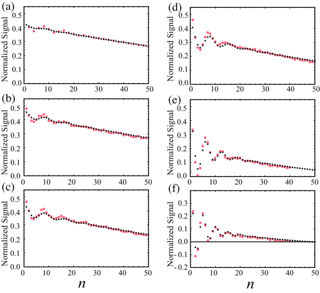
Figure 7: Measured (large red) and simulated QZE experiments (small black) with $\tau_{xy}=$ (a) 0.1, (b) 0.2, (c) 0.3, (d) 0.5, (e) 1.0, and (f) 1.5 ms in the case of $\tau_{z}=1.0$ ms. The $x$-axis indicates $n$’th measurement. We take $M_{-}(\tau_{z})$ as a “measurement” in Eq. (19). $(T_{d},1/p_{s})=(6.5,300)$ ms. $T/N_{t}=0.1$ ms is taken for simulations during $\tau_{xy}$ and $\tau_{z}$.

The results with $\tau_{xy}\leq 0.2$ ms in figure 6 are largely distorted from the FID signal. On the other hand, a more oscillatory behaviour is observed for large $\tau_{xy}$ values, as seen in figure 7. These oscillations are originated from the $J$-coupling and the large oscillations indicate that the QZE is less effective. Therefore, $\tau_{xy}=0.3$ ms is the optimal measurement frequency for the QZE demonstration with our imperfect measurement of $M_{-}(1.0~{}{\rm ms})$ [31].

We vary $\tau_{z}$ from 0.8, 1.0, 1.2, 1.5, 2.0, and 2.5 ms in $M_{\pm}(\tau_{z})$ with the constant $\tau_{xy}=0.3$ ms, as shown in figure 8. The simulations with $M_{+}(\tau_{z})$ are very similar to those with $T_{1s}=\infty$ (without longitudinal relaxation of the ¹³C spin). It can be understood as follows. The state during $\tau_{z}$ is very close to $\rho_{\rm th}$ in the case of $M_{+}(\tau_{z})$. The longitudinal relaxation given as Eq. (16) is not effective in this case since the state during $\tau_{z}$ are almost the same as $\rho_{\rm th}$. On the contrary, the state during $\tau_{z}$ is very close to $|1\rangle\langle 1|\otimes\sigma_{0}/2$ in the case of $M_{-}(\tau_{z})$. This process transforms the state $|1\rangle\langle 1|\otimes\sigma_{0}/2$ to $|0\rangle\langle 0|\otimes\sigma_{0}/2=\rho_{\rm th}$, which means the relaxation is more effective in this case. We are able to avoid most of the unwanted effects of longitudinal relaxation on the ¹³C spin dynamics during $\tau_{z}$ taking $M_{+}(\tau_{z})$ as a measurement. The longer $\tau_{z}$ leads to fewer oscillations of the signal, as seen in figure 8. This shows that $\tau_{z}\sim 2.5$ ms is long enough to implement the non-selective measurement.

The signals with $M_{+}(\tau_{z})$ decay slower than the envelope of the FID signal, as shown in figure  8. This fact shows that the dephasing of ¹³C spin is reduced by the QZE, since the decay of the FID signal is caused by the dephasing of the ¹³C spin, as discussed in § 2.2. It is worth mentioning that, the only difference between the figures 6 and 8 are the existence of the entangling operations (measurements by the device), and the suppression of the decoherence in the figure 8 comes from the implementation of the measurements. Further, a single set of parameters $(T_{d},1/p_{s})=(6.5,300)$ ms for the simulations can reproduce all the experimental results well, as shown in figures 3, 7, and 8.

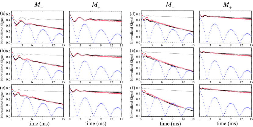
Figure 8: Measured (large red) and simulated QZE experiments (small black) with $\tau_{z}=$ (a) 0.8, (b) 1.0, (c) 1.2, (d) 1.5, (e) 2.0, and (f) 2.5 ms in the case of $\tau_{xy}=0.3$ ms. The $x$-coordinate of the $n$’th point is calculated from $n\tau_{xy}$ without taking into account the measurement times $\sim n\tau_{z}$. $(T_{d},1/p_{s})=(6.5,300)$ ms. $T/N_{t}=0.1$ ms is taken, while the pulse duration is 58 $\mu$s. The solid lines are simulations when $T_{1s}=\infty$. The absolute values of the measured FID signals ($\times$’s) are also plotted for comparison.

4 Conclusion and Discussions

We successfully suppressed the dephasing of an ensemble of spins through the application of sequential non-selective measurements. Note that these measurements does not rely on the ensemble nature of NMR. This is a proof-of-principle demonstration of the Quantum Zeno Effect suppressing non-unitary evolution.

One interesting extension of this work would be the protection of an arbitrary unknown state, as discussed in the early stages of quantum information processing [34]. Here, we propose a scheme for a specific case, when $|\psi_{i}\rangle=\alpha|0\rangle+\beta|1\rangle$ is protected.

We encode $|\psi_{i}\rangle\langle\psi_{i}|$ to a two-qubit state by adding an ancillary qubit, as

$$\rho=|\psi\rangle\langle\psi|,$$ (21)

where, $|\psi\rangle=\alpha|++\rangle+\beta|--\rangle$.

The decoherence is described with the operator sum formalism as

$$\rho^{\prime} = (1-\epsilon)\rho+\frac{1}{2}\epsilon|\psi_{d}\rangle\langle\psi_{d}|+\frac{1}{2}\epsilon|\psi^{\prime}_{d}\rangle\langle\psi^{\prime}_{d}|,$$ (22)

where $|\psi_{d}\rangle$ $=$ $\alpha|-+\rangle+\beta|+-\rangle$ and $|\psi^{\prime}_{d}\rangle$ $=$ $\alpha|+-\rangle+\beta|-+\rangle$.

Since the error rate $\epsilon$ is supposed to be small, we ignore the terms of order $\epsilon^{2}$ or higher. We assume a quadratic decay of the first qubit, or $\epsilon=\Gamma^{2}t^{2}$, where $t$ is the interval between the measurements. Then, we perform the following projection operator

$$P_{\rm even} = |++\rangle\langle++|+|--\rangle\langle--|$$ (23)

and we obtain

$$\rho^{\prime\prime} = (1-\epsilon)\rho,$$ (24)

although realization of $P_{\rm even}$ is an experimental challenge. One possible implementation of $P_{\rm even}$ is to use a third qubit. If we measure nonselectively this third qubit, after we entangle the third qubit with the first and second qubits, this provides us with a parity projection. When we repeat this procedure $N$-times in the period $T$, then $\rho_{T}$ at the time $T$ is

$$\rho_{T} = \left(1-\Gamma^{2}\left(\frac{T}{N}\right)^{2}\right)^{N}\rho.$$ (25)

In the limit of infinite $N$, we obtain $\rho_{T}=\rho$. $\rho_{T}$ may be decoded to obtain $|\psi_{i}\rangle$ back.

References

References

- [1] Nakazato H, Namiki M and Pascazio S 1996 Int. J. Mod. Phys. B 10 247
- [2] Palma G M, Suominen K A and Ekert A K 1996 Proc. Roy. Soc. London Ser. A 452 567
-
[3]
Misra B and Sudarshan E C G 1977 J. Math. Phys.
18 756
see also a recent review paper by Facchi P and Pascazio S 2008 J. of Phys. A: Math. and Theor. 41, 493001 references therein - [4] Nakazato H, Takazawa T and Yuasa K 2003 Phys. Rev. Lett. 90 060401
- [5] Matsuzaki Y, Benjamin S C and Fitzsimons J 2011 Phys. Rev. A. 84 012103
- [6] Chin A W, Huelga S F and Plenio M B 2012 Phys. Rev. Lett. 109 233601
- [7] Kwiat P, Weinfurter H, Herzog T, Zeilinger A and Kasevich M A 1995 Phys. Rev. Lett. 74 4763
- [8] See, for example, Facchi P and Pascazio S 2008 J. Phys. A: Math. Theor. 41 493001 references therein
- [9] Lidar D A, Review of Decoherence-Free Subspaces, Noiseless Subsystems, and Dynamical Decoupling, in Quantum Information and Computation for Chemistry: Advances in Chemical Physics Volume 154 (ed S. Kais), (John Wiley & Sons, Hoboken, New Jersey) references therein
- [10] Itano W M, Heinzen D J, Bollinger J J and Wineland D J 1990 Phys. Rev. A 41 2295
- [11] Xiao L and Jones J 2006 Physics Letters A 359 424
- [12] Streed E W, Mun J, Boyd J, Campbell G K, Medley P, Ketterle W and Pritchard D E 2006 Phys. Rev. Lett. 97 260402
- [13] Bernu J, Deléglise S, Sayrin C, Kuhr S, Dotsenko I, Brune M, Raimond J M and Haroche S 2008 Phys. Rev. Lett. 101 180402
- [14] Schafer F, et al. 2014 Nature communications 5 3194
- [15] Fischer M C, Gutiérrez-Medina B and Raizen M G 2001 Phys. Rev. Lett. 87 040402
- [16] Álvarez G A, Rao D D B, Frydman L and Kurizki G 2010 Phys. Rev. Lett. 105 160401
-
[17]
Matsuzaki Y, Saito S, Kakuyanagi Kand Semba K
2010
Phys. Rev. B 82 180518
Matsuzaki Y and Tanaka H 2012 arXiv:1209.3136
Matsuzaki Y and Tanaka H 2016 J. Phys. Soc. Jpn. 85 014001 - [18] Balzer C, Hannemann Th, Reiß D, Wunderlich Chr, Neuhauser W, and Toschek P E 2002 Opt. Commun. 211 235, Toschek P E and Wunderlich Ch 2001 Eur. Phys. J. D 14 387
- [19] See, for example, Kondo Y et al. 2007 J. Phys. Soc. Jpn. 76 074002 references therein
- [20] Gardiner C W and Zoller P, Quantum noise: a handbook of Markovian and non-Markovian quantum stochastic methods with applications to quantum optics, Vol. 56, (Springer, 2004)
- [21] See, for example, Abragam A, Principles of Nuclear Magnetism, (Oxford University Press, New York, 1989)
- [22] Levitt M H, Spin Dynamics, (John Wiley and Sons, New York, 2008)
- [23] Zurek W H 2003 Rev. Mod. Phys. 75 715
- [24] Nielsen M A and Chuang I L, Quantum Computation and Quantum Information (Cambridge University Press, 2000)
- [25] See, for example, De Lange G, et al. 2010 Science 330 Issue 6000 60 references therein
- [26] Barnum H, Nielsen M A and Schumacher B 1998 Phys. Rev. A 57 4153
- [27] Nakahara M, Kondo Y, Hata K and Tanimura S 2004 Phys. Rev. A 70 052319
- [28] Ali Ahmed M A, Álvarez G A and Suter D 2013 Phys. Rev. A 87 042309 references therein
- [29] Gullion T, Baker D B and Conradi M S 1990 J. Magn. Reson. 89 479
-
[30]
Yuge T, Sasaki S and Hirayama Y 2011 Phys. Rev. Lett.
107 170504
Álvarez G A and D. Suter 2011 Phys. Rev. Lett. 107 230501 - [31] Facchi F, Nakaguro Y, Nakazato H, Pascazio S, Unoki M, and Yuasa K 2003 Phys. Rev. A 68 012107
- [32] Kondo Y 2007 J. Phys. Soc. Jpn. 76 104004
- [33] Cummins H K, Llewellyn G, and Jones J A 2003 Phys. Rev. A 67 042308
- [34] Barenco A, Berthiaume A, Deutsch D, Ekert A, Jozsa R and Macchiavello C 1997 S. I. A. M. Journal on Computing 26-5 1541