Spatial discretization error in Kalman filtering for discrete-time infinite dimensional systems

Abstract.

We derive a reduced-order state estimator for discrete-time infinite dimensional linear systems with finite dimensional Gaussian input and output noise. This state estimator is the optimal one-step estimate that takes values in a fixed finite dimensional subspace of the system’s state space — consider, for example, a Finite Element space. We then derive a Riccati difference equation for the error covariance and use sensitivity analysis to obtain a bound for the error of the state estimate due to the state space discretization.

1. Introduction

In this paper, we consider the state estimation problem for infinite dimensional discrete time linear systems with finite dimensional Gaussian input and output noise. The objective is to find the optimal one-step state estimate from a given subspace of the original state space (for example a Finite Element space). We shall also find a bound for the error due to the spatial discretization to the state estimate at the infinite time limit.

The dynamics of the system under consideration is given by

(1) $$\begin{cases}x_{k}=Ax_{k-1}+Bu_{k},\\ y_{k}=Cx_{k}+w_{k},\\ x_{0}\sim N(m,S_{0})\end{cases}$$

where $x_{k}\in\mathcal{X}$, $A\in\mathcal{L}(\mathcal{X})$, $B\in\mathcal{L}(\mathbb{C}^{q},\mathcal{X})$, and $C\in\mathcal{L}(\mathcal{X},\mathbb{C}^{m})$. The state space $\mathcal{X}$ is a separable Hilbert space. The noise processes are assumed to be Gaussian, $u_{k}\sim N(0,U)$ and $w_{k}\sim N(0,R)$ where $U\in\mathbb{R}^{q\times q}$ and $R\in\mathbb{R}^{m\times m}$ are positive-definite and symmetric. It is also assumed that $u$, $w$, and $x_{0}$ are mutually independent, and the noises at different times are independent.

When measurements $y_{j}$ for $j=1,...,k$ are known, the state estimate $\hat{x}_{k}$ minimizing the conditional expectation $\mathbb{E}\!\left(\left|\!\left|\hat{x}_{k}-x_{k}\right|\!\right|_{\mathcal{X}}^{2}\Big{|}\{y_{j},\,j=1,...,k\}\right)$ is given by $\hat{x}_{k}=\mathbb{E}\!\left(x_{k}|\{y_{j},\,j\leq k\}\right)$. In the presented Gaussian case, the conditional expectation $\hat{x}_{k}$ can be computed recursively from $\hat{x}_{k-1}$ and $y_{k}$. This recursive scheme is known as the Kalman filter, originally presented in [12] in the finite dimensional setting. For infinite dimensional systems, the generalization is straightforward and it can be done, for example, using the presentation by Bogachev [4: Section 3.10] or the more explicit presentation [14] by Krug. Let us present a short introduction. It is well known that linear combinations of Gaussian random variables are also Gaussian random variables. Further, if $\left[\begin{matrix}h_{1}\\ h_{2}\end{matrix}\right]\sim N\left(\left[\begin{matrix}m_{1}\\ m_{2}\end{matrix}\right],\left[\begin{matrix}P_{11}&P_{12}\\ P_{12}^{*}&P_{22}\end{matrix}\right]\right)$ where $h_{1}\in\mathcal{X}$ and $h_{2}$ is finite dimensional, then

(2) $$\mathbb{E}\!\left(h_{1}|h_{2}\right)=m_{1}+P_{12}P_{22}^{+}(h_{2}-m_{2})$$

and

(3) $$\textup{Cov}\left[h_{1}-\mathbb{E}\!\left(h_{1}|h_{2}\right),h_{1}-\mathbb{E}\!\left(h_{1}|h_{2}\right)\right]=P_{11}-P_{12}P_{22}^{+}P_{12}^{*}.$$

Remark that $\textup{Cov}\left[\mathbb{E}\!\left(h_{1}|h_{2}\right),\mathbb{E}\!\left(h_{1}|h_{2}\right)\right]=P_{12}P_{22}^{+}P_{12}^{*}$ so that in fact,

(4) $$\textup{Cov}\left[h_{1}-\mathbb{E}\!\left(h_{1}|h_{2}\right),h_{1}-\mathbb{E}\!\left(h_{1}|h_{2}\right)\right]$$

$$\hskip 28.45274pt=\textup{Cov}\left[h_{1},h_{1}\right]-\textup{Cov}\left[\mathbb{E}\!\left(h_{1}|h_{2}\right),\mathbb{E}\!\left(h_{1}|h_{2}\right)\right].$$

Applying (2) and (3) to the jointly Gaussian random variable $[x_{k},y_{1},...,y_{k}]$ and the block matrix inversion formula

(5) $$\!\left[\begin{smallmatrix}F\!&G\!\\ G^{T}&H\end{smallmatrix}\right]^{\!-1}\!\!=\left[\begin{smallmatrix}F^{-1}\!+F^{-1}G(H\!-G^{T}F^{-1}G)^{-1}G^{T}F^{-1}&-F^{-1}G(H\!-G^{T}F^{-1}G)^{-1}\\ -(H-G^{T}F^{-1}G)^{-1}G^{T}F^{-1}&(H-G^{T}F^{-1}G)^{-1}\end{smallmatrix}\right]$$

to $P_{22}\,\widehat{=}\,\textup{Cov}\left[[y_{1},...,y_{k}],[y_{1},...,y_{k}]\right]$ eventually leads to the full state Kalman filter equations

(6) $$\hat{x}_{k}=A\hat{x}_{k-1}+K_{k}^{(F)}(y_{k}-CA\hat{x}_{k-1})$$

where $K_{k}^{(F)}$ for $k=1,2,...$ are called Kalman gains, and they are given by $K_{k}^{(F)}=\tilde{P}_{k}^{(F)}C^{*}(C\tilde{P}_{k}^{(F)}C^{*}+R)^{-1}$, and the Riccati difference equation (RDE)

(7) $$\begin{cases}\tilde{P}_{k}^{(F)}=AP_{k-1}^{(F)}A^{*}+BUB^{*},\\ P_{k}^{(F)}=\tilde{P}_{k}^{(F)}-\tilde{P}_{k}^{(F)}C^{*}(C\tilde{P}_{k}^{(F)}C^{*}+R)^{-1}C\tilde{P}_{k}^{(F)}.\end{cases}$$

Here $P_{k}^{(F)}=\textup{Cov}\left[x_{k}-\hat{x}_{k},x_{k}-\hat{x}_{k}\right]$ is the (estimation) error covariance and $\tilde{P}_{k}^{(F)}=\textup{Cov}\left[x_{k}-\mathbb{E}\!\left(x_{k}|[y_{1},...,y_{k-1}]\right),x_{k}-\mathbb{E}\!\left(x_{k}|[y_{1},...,y_{k-1}]\right)\right]$ is the prediction error covariance. The initial values are $\hat{x}_{0}=m$ and $P_{0}^{(F)}=S_{0}$. The superscript $(F)$ refers to full Kalman filter estimate and it is used for later purposes.

Numerical implementation of the Kalman filter to infinite dimensional systems requires discretization of the state space. If the implementation is then carried out directly to the discretized system, the result is not optimal. In particular, if the state estimation is performed online, the restrictions in computing power might prevent using a very fine mesh for the simulations. In such cases it is beneficial to take the discretization error into account in the state estimation. The purpose of this paper is to derive the optimal one-step state estimate that takes values in the discretized state space, and to analyze the discrepancy between the proposed state estimate and the full state Kalman filter estimate.

We tackle this task in Section 2 by first fixing the structure of the filter in (8). In the spirit of Kalman filtering, we require that the $k^{\textrm{th}}$ estimate depends only on the previous estimate and the current measured output $y_{k}$. We then find the expression for a filter with such structure. The rest of the paper is organized as follows: In Section 3, we derive a Riccati difference equation for the estimation error covariance for the proposed method. Compared to (7), this equation contains an additional term due to the discretization. In Section 4, we use sensitivity analysis for algebraic Riccati equations — developed by Sun in [23] — to determine a bound for the error due to the discretization at the infinite time limit. In short, it is shown that when the approximation properties of the subspace improve at some rate as the spatial discretization is refined, then the finite dimensional state estimate converges to the full state Kalman filter estimate at least with the same convergence rate. In Section 5, the proposed method is implemented to one dimensional wave equation with damping, and the result is compared with the Kalman filter that does not take into account the spatial discretization error.

The “engineer’s approach”, i.e., the direct Kalman filter implementation to the discretized system is studied in [1] by Bensoussan and in [7] by Germani et al. The latter contains a convergence result for the finite dimensional state estimate (in continuous time) with a convergence rate estimate. They also show convergence of the solutions of the corresponding Riccati differential equations in the space of continuous Hilbert-Schmidt operator-valued functions. A method where the discretization error is taken into account is proposed by Pikkarainen in [17]. Their approach is based on keeping track of the discretization error mean and covariance. Then with certain approximations on the error distributions, they too end up with a one-step method that is numerically implemented in [11] by Huttunen and Pikkarainen.

Our method is very closely related to the reduced-order filtering methods that have been studied since the introduction of the Kalman filter itself; see e.g., [2; 3; 19; 20; 22]. The articles by Bernstein and Hyland, [2; 3] yield a state estimator similar to ours for continuous time. They obtain algebraic optimality equations for the error covariance and Kalman gain limits as the time index $k\to\infty$, in terms of “optimal projections”. Our solution is somewhat more straightforward, and we obtain the error covariances and Kalman gains for all time steps. A similar method is developed by Simon in [19] with a more restrictive assumption on the filter structure. For a more thorough introduction and review on the earliest results on reduced-order filtering techniques, we refer to [22] by Stubberud and Wismer and to [20] by Sims.

Infinite dimensional Kalman filter has numerous applications. The practical application that motivated the paper [17] is the electrical impedance process tomography, studied by Seppänen et al. in [18]. Infinite dimensional Kalman filter implementation to optical tomography problem can be found in [9] by Hiltunen et al. Quasiperiodic phenomena is studied by Solin and Särkkä in [21] using the infinite dimensional Kalman filter. They use a weather prediction model and fMRI brain imaging as example cases. The numerical treatment is done using truncated eigenbasis approach instead of using FEM as in the example of this article.

Notation

We denote by $\mathcal{L}(\mathcal{X}_{1},\mathcal{X}_{2})$ the space of bounded linear operators from $\mathcal{X}_{1}$ to $\mathcal{X}_{2}$, and $\mathcal{L}(\mathcal{X})=\mathcal{L}(\mathcal{X},\mathcal{X})$. The subspace of self-adjoint operators in $\mathcal{X}$ is denoted by $\mathcal{L}^{*}(\mathcal{X})$. The spectrum of an operator is denoted by $\sigma(\cdot)$. The sigma algebra generated by a random variable (or random variables) is denoted by $\mathcal{S}(\cdot)$. The Moore-Penrose pseudoinverse of a matrix $T$ is denoted by $T^{+}$.

The covariance of square integrable random variables $x_{1}\in\mathcal{X}_{1}$ and $x_{2}\in\mathcal{X}_{2}$ is the operator in $\mathcal{L}(\mathcal{X}_{2},\mathcal{X}_{1})$ defined for $h\in\mathcal{X}_{2}$ by
$\textup{Cov}\left[x_{1},x_{2}\right]h:=\mathbb{E}\!\left((x_{1}-\mathbb{E}\!\left(x_{1}\right))\left<x_{2}-\mathbb{E}\!\left(x_{2}\right),h\right>_{\mathcal{X}_{2}}\right)$.

2. The reduced-order state estimate

Let $\Pi_{s}:\mathcal{X}\to\mathcal{X}$ be an orthogonal projection from the state space $\mathcal{X}$ (a separable, complex Hilbert space) to an $n$-dimensional subspace of $\mathcal{X}$ (e.g., a finite element space). Assume we have a coordinate system in $\mathbb{C}^{n}$ associated to this subspace, such that the inner product is preserved, and denote by $\Pi:\mathcal{X}\to\mathbb{C}^{n}$ the representation of the projection $\Pi_{s}$ in this coordinate system. That is, $\left<\Pi_{s}x_{1},\Pi_{s}x_{2}\right>_{\mathcal{X}}=\left<\Pi x_{1},\Pi x_{2}\right>_{\mathbb{C}^{n}}$ for $x_{1},x_{2}\in\mathcal{X}$. Then it holds that $\Pi\Pi^{*}=I\in\mathbb{C}^{n\times n}$ and $\Pi^{*}\Pi=\Pi_{s}$.

Finding an exact solution to the estimation problem of the finite dimensional $\Pi x_{k}$ would require solving the full state Kalman filtering problem and then projecting the estimate by $\Pi$. This, of course, doesn’t make much practical sense. As mentioned above, we want to find the optimal state estimate $\tilde{x}_{k}$ in $\Pi_{s}\mathcal{X}$ that can be computed from the previous state estimate $\tilde{x}_{k-1}$ and the current measurement $y_{k}$. More precisely, we want to obtain $\tilde{x}_{k}$’s satisfying

(8) $$\begin{cases}\tilde{x}_{0}=\Pi m,\\ \tilde{x}_{k}=\Pi\mathbb{E}\!\left(x_{k}|\tilde{x}_{k-1},y_{k}\right),\qquad k\geq 1,\end{cases}$$

where $x_{k}$ satisfy (1). One thing to notice here is that in contrast to the full state filtering, the conditioning is not done over a filtration, because — loosely speaking — we lose some information when we only take into account the last measurement and the last estimate of the state projection. Without loss of generality, we may assume that $m=0$ (see Remark 2.1). Note that this also implies $\mathbb{E}\!\left(x_{k}\right)=0$ and further, $\mathbb{E}\!\left(\tilde{x}_{k}\right)=0$ and $\mathbb{E}\!\left(y_{k}\right)=0$ for all $k\geq 1$.

We then proceed to find a concrete representation for $\tilde{x}_{k}$. From (8) it can be inductively deduced that $[x_{k-1},\tilde{x}_{k-1}]$ is Gaussian and from (1), also $[x_{k},\tilde{x}_{k-1},y_{k}]$ is Gaussian. The reasoning leading to the full state Kalman filter equations utilizing equations (2) and (3) together with the block matrix inversion formula (5) can be generalized for any Gaussian random variable $[h_{1},h_{2},h_{3}]$ with $h_{1}\in\mathcal{X}$, and $h_{2}$ and $h_{3}$ finite dimensional, to obtain

(9) $$\mathbb{E}\!\left(h_{1}|h_{2},h_{3}\right)= \mathbb{E}\!\left(h_{1}|h_{2}\right)+\textup{Cov}\left[h_{1}-\mathbb{E}\!\left(h_{1}|h_{2}\right),h_{3}-\mathbb{E}\!\left(h_{3}|h_{2}\right)\right]\times$$

$$\times\textup{Cov}\left[h_{3}-\mathbb{E}\!\left(h_{3}|h_{2}\right),h_{3}-\mathbb{E}\!\left(h_{3}|h_{2}\right)\right]^{-1}(h_{3}-\mathbb{E}\!\left(h_{3}|h_{2}\right)).$$

The corresponding equation can be obtained for the covariance operator. The full state Kalman filter equations (6) and (7) are obtained by applying (9) to $h_{1}=x_{k}$, $h_{2}=[y_{1},...,y_{k-1}]$, and $h_{3}=y_{k}$. In what follows, we obtain $\tilde{x}_{k}$ by applying (9) to $h_{1}=x_{k}$, $h_{2}=\tilde{x}_{k-1}$, and $h_{3}=y_{k}$.

Since $m=0$, there exists an operator $Q_{k-1}\in\mathcal{L}(\mathbb{R}^{n},\mathcal{X})$ such that

(10) $$\mathbb{E}\!\left(x_{k-1}|\tilde{x}_{k-1}\right)=Q_{k-1}\tilde{x}_{k-1}$$

and the (estimation) error covariance

(11) $$P_{k-1}:=\textup{Cov}\left[x_{k-1}-Q_{k-1}\tilde{x}_{k-1},x_{k-1}-Q_{k-1}\tilde{x}_{k-1}\right].$$

Using these we can make an orthogonal decomposition of the state

$$x_{k-1}=\mathbb{E}\!\left(x_{k-1}|\tilde{x}_{k-1}\right)+\left(x_{k-1}-\mathbb{E}\!\left(x_{k-1}|\tilde{x}_{k-1}\right)\right)=:Q_{k-1}\tilde{x}_{k-1}+v_{k-1}$$

where $v_{k-1}\sim N\big{(}0,P_{k-1}\big{)}$ and it is independent of the estimate $\tilde{x}_{k-1}$. Together with (1), this gives decompositions for the state $x_{k}$ and output $y_{k}$:

(12) $$\begin{cases}x_{k}=Ax_{k-1}+Bu_{k}=A(Q_{k-1}\tilde{x}_{k-1}+v_{k-1})+Bu_{k},\\ y_{k}=Cx_{k}+w_{k}=C(A(Q_{k-1}\tilde{x}_{k-1}+v_{k-1})+Bu_{k})+w_{k}\end{cases}$$

from which one can deduce $\mathbb{E}\!\left(x_{k}|\tilde{x}_{k-1}\right)=AQ_{k-1}\tilde{x}_{k-1}$ and $\mathbb{E}\!\left(y_{k}|\tilde{x}_{k-1}\right)=CAQ_{k-1}\tilde{x}_{k-1}$.

Then we need the two covariances in (9). To this end, define the prediction error covariance for which we get a representation from (12),

(13) $$\tilde{P}_{k}:=\textup{Cov}\left[x_{k}-\mathbb{E}\!\left(x_{k}|\tilde{x}_{k-1}\right),x_{k}-\mathbb{E}\!\left(x_{k}|\tilde{x}_{k-1}\right)\right]=AP_{k-1}A^{*}+BUB^{*}.$$

Using the two equations in (12), we get

$$\textup{Cov}\left[x_{k}-\mathbb{E}\!\left(x_{k}|\tilde{x}_{k-1}\right),y_{k}-\mathbb{E}\!\left(y_{k}|\tilde{x}_{k-1}\right)\right]=\tilde{P}_{k}C^{*}$$

and the covariance of output prediction error from the second equation in (12)

$$\textup{Cov}\left[y_{k}-\mathbb{E}\!\left(y_{k}|\tilde{x}_{k-1}\right),y_{k}-\mathbb{E}\!\left(y_{k}|\tilde{x}_{k-1}\right)\right]=C\tilde{P}_{k}C^{*}+R.$$

Now we have all the components for obtaining $\tilde{x}_{k}$ by (9),

(14) $$\mathbb{E}\!\left(x_{k}|\tilde{x}_{k-1},y_{k}\right)=AQ_{k-1}\tilde{x}_{k-1}+\underbrace{\tilde{P}_{k}C^{*}\big{(}C\tilde{P}_{k}C^{*}\!+R\big{)}^{-1}}_{=:K_{k}}(y_{k}\!-CAQ_{k-1}\tilde{x}_{k-1}).$$

It remains to compute the error covariance $P_{k}$ defined in (11), and the operator $Q_{k}$ defined through (10). By (4), $P_{k}$ is given by

$$P_{k}=S_{k}-Q_{k}\tilde{S}_{k}Q_{k}^{*}$$

where $S_{k}=\textup{Cov}\left[x_{k},x_{k}\right]$ is the state covariance and $\tilde{S}_{k}=\textup{Cov}\left[\tilde{x}_{k},\tilde{x}_{k}\right]$ is the state estimate covariance. The state $x_{k}$ is a linear combination of mutually independent Gaussian random variables $x_{k-1}$ and $u_{k}$ and so $S_{k}$ can be obtained from the Lyapunov difference equation

(15) $$S_{k}=AS_{k-1}A^{*}+BUB^{*}$$

and the first one, $S_{0}$, is the initial state covariance in (1). Also, by (12),

(16) $$y_{k}-CAQ_{k-1}\tilde{x}_{k-1}=CAv_{k}+CBu_{k}+w_{k}\sim N\big{(}0,C\tilde{P}_{k}C^{*}+R\big{)}$$

where $v_{k}$, $u_{k}$, and $w_{k}$ are mutually independent and also independent with the state estimate $\tilde{x}_{k-1}$. Thus, by (14), also $\tilde{S}_{k}$ is obtained from a Lyapunov difference equation,

(17) $$\tilde{S}_{k}=\Pi AQ_{k-1}\tilde{S}_{k-1}Q_{k-1}^{*}A^{*}\Pi^{*}+\Pi K_{k}\big{(}C\tilde{P}_{k}C^{*}+R\big{)}(\Pi K_{k})^{T}$$

with $\tilde{S}_{0}=0$.

By (2), $Q_{k}$ is given by

(18) $$Q_{k}=\textup{Cov}\left[x_{k},\tilde{x}_{k}\right]\tilde{S}_{k}^{-1}.$$

The case when $\tilde{S}_{k}$ is not invertible is discussed in Remark 2.2. The cross covariance operator $V_{k}:=\textup{Cov}\left[x_{k},\tilde{x}_{k}\right]$ in (18) can be computed by “anchoring” $x_{k}$ and $\tilde{x}_{k}$ to $\tilde{x}_{k-1}$ using equations (12) and (14) and the fact that $Av_{k-1}+Bu_{k}\sim N\big{(}0,\tilde{P}_{k}\big{)}$,

$$\textup{Cov}\left[x_{k},\tilde{x}_{k}\right]=AQ_{k-1}\tilde{S}_{k-1}Q_{k-1}^{*}A^{*}\Pi^{*}+\tilde{P}_{k}C^{*}\big{(}C\tilde{P}_{k}C^{*}+R\big{)}^{-1}C\tilde{P}_{k}\Pi^{*}.$$

It is worth noting here that $\tilde{S}_{k}=\Pi\textup{Cov}\left[x_{k},\tilde{x}_{k}\right]$ implying the intuitive fact, $\Pi Q_{k}=I$ in the case that $\tilde{S}_{k}$ is invertible.

Let us conclude by presenting some remarks concerning the derivation of the reduced-order state estimate and then collecting the relevant equations to an algorithm.

Remark 2.1.

The assumption $m=0$ does not restrict generality, since we can always always add $\Pi A^{k}m$ to $\tilde{x}_{k}$ and subtract $CA^{k}m$ from $y_{k}$ in (12). However, this is how to make the derivation accurate. In practical implementation, it is reasonable to just start the state estimate from $\tilde{x}_{0}=\Pi m$ and then proceed as described.

Remark 2.2.

If $\tilde{S}_{k}$ is not invertible, it means that $\mathcal{R}(\tilde{S}_{k})$, the range of $\tilde{S}_{k}$, does not cover the whole space $\mathbb{C}^{n}$. The estimate $\tilde{x}_{k}$ lies on $\mathcal{R}(\tilde{S}_{k})$ almost surely. Thus $Q_{k}$ is not determined uniquely in this case. By imposing additional requirements $\Pi Q_{k}=I$ and ${(I-\Pi_{s})Q_{k}}\big{|}_{\mathcal{R}(\tilde{S}_{k})^{\bot}}=0$ then $Q_{k}$ is uniquely determined and it is given by $Q_{k}=\tilde{Q}_{k}+\Pi^{*}(I-\Pi\tilde{Q}_{k})=\Pi^{*}+(I-\Pi_{s})\tilde{Q}_{k}$ where $\tilde{Q}_{k}=\textup{Cov}\left[x_{k},\tilde{x}_{k}\right]\tilde{S}_{k}^{+}$.

Algorithm 2.3.

As with the full state Kalman filter, the following operator-valued equations can be computed beforehand (offline):

$$S_{k} =AS_{k-1}A^{*}+BUB^{*},$$

$$\tilde{P}_{k} =AP_{k-1}A^{*}+BUB^{*},$$

$$K_{k} =\tilde{P}_{k}C^{*}\big{(}C\tilde{P}_{k}C^{*}\!+R\big{)}^{-1},$$

$$V_{k} =AQ_{k-1}\tilde{S}_{k-1}Q_{k-1}^{*}A^{*}\Pi^{*}+K_{k}\big{(}C\tilde{P}_{k}C^{*}+R\big{)}(\Pi K_{k})^{T},$$

$$\tilde{S}_{k} =\Pi V_{k},$$

$$Q_{k} =\Pi^{*}+(I-\Pi_{s})\tilde{S}_{k}^{+}V_{k},$$

$$P_{k} =S_{k}-Q_{k}\tilde{S}_{k}Q_{k}^{*}.$$

The initial values are $S_{0}$ (given in (1)), $P_{0}=S_{0}$, $\tilde{S}_{0}=0$, and $Q_{0}=\Pi^{*}$. The state estimate is given by

$$\tilde{x}_{0} =\Pi m,$$

$$\tilde{x}_{k} =\Pi AQ_{k-1}\tilde{x}_{k-1}+\Pi K_{k}(y_{k}-CAQ_{k-1}\tilde{x}_{k-1}).\hskip 19.91692pt$$

Practical implementation of the proposed method is discussed in Section 6.1. An alternative equation for $P_{k}$ is derived in the following section.

3. The error covariance equation

Motivated by the main theorem of [2], we next seek for a Riccati difference equation satisfied by the error covariance $P_{k}$. This equation will be needed later for determining a bound for the error in the state estimate due to the spatial discretization. To this end, define the augmented state $\bar{x}_{k}:=\left[\begin{matrix}x_{k}\\ \tilde{x}_{k}\end{matrix}\right]$ for which we have dynamic equations

$$\!\left[\begin{matrix}x_{k}\\ \tilde{x}_{k}\end{matrix}\right]\! =\!\left[\!\!\begin{array}[]{cc}A&0\\ \Pi K_{k}CA&\Pi(A-K_{k}CA)Q_{k-1}\end{array}\!\!\!\right]\!\!\left[\begin{matrix}x_{k-1}\\ \tilde{x}_{k-1}\end{matrix}\right]+\left[\!\!\begin{array}[]{cc}B&0\\ \Pi K_{k}CB&\Pi K_{k}\end{array}\!\!\right]\!\!\left[\begin{matrix}u_{k}\\ w_{k}\end{matrix}\right]$$

$$=:\bar{A}_{k}\bar{x}_{k-1}+\bar{B}_{k}\bar{u}_{k}.$$

The augmented state covariance satisfies the Lyapunov difference equation

(19) $$\bar{S}_{k}=\bar{A}_{k}\bar{S}_{k-1}\bar{A}_{k}^{*}+\bar{B}_{k}\bar{U}\bar{B}_{k}^{*}$$

where $\bar{U}=\left[\begin{matrix}U&0\\ 0&R\end{matrix}\right]$. This covariance can be written as a block operator by $\bar{S}_{k}=\left[\begin{matrix}S_{k}&V_{k}\\ V_{k}^{*}&\tilde{S}_{k}\end{matrix}\right]$ where $S_{k}$ and $\tilde{S}_{k}$ are the state and state estimate covariances, given in (15) and (17), respectively. Now it holds that $Q_{k}=V_{k}\tilde{S}_{k}^{-1}$ (or $Q_{k}=V_{k}\tilde{S}_{k}^{+}+\Pi^{*}(I-\Pi V_{k}\tilde{S}_{k}^{+})$ if $\tilde{S}_{k}$ is not invertible) and thus for the reduced-order error covariance defined in (11), it holds that $P_{k}=S_{k}-V_{k}\tilde{S}_{k}^{+}V_{k}^{*}$. Also, for the prediction error covariance we have $\tilde{P}_{k}=A(S_{k}-V_{k}\tilde{S}_{k}^{+}V_{k}^{*})A^{*}+BUB^{*}$ by (13). Using these notations we get from (19)

$$V_{k} =AS_{k-1}A^{*}C^{*}K^{*}\Pi^{*}+AV_{k-1}\tilde{S}_{k-1}^{+}V_{k-1}^{*}A^{*}(\Pi-\Pi K_{k}C)^{*}+BUB^{*}C^{*}K_{k}^{*}\Pi^{*}$$

$$=\tilde{P}_{k}C^{*}(C\tilde{P}_{k}C^{*}+R)^{-1}C\tilde{P}_{k}\Pi^{*}+AV_{k-1}\tilde{S}_{k-1}^{+}V_{k-1}^{*}A^{*}\Pi^{*},$$

and similarly $\tilde{S}_{k}=\Pi V_{k}=V_{k}^{*}\Pi^{*}$. Using the state covariance Lyapunov equation (15) and the equations above and noting that $V_{k}\tilde{S}_{k}^{+}V_{k}^{*}=Q_{k}V_{k}^{*}=V_{k}Q_{k}^{*}=Q_{k}\tilde{S}_{k}Q_{k}^{*}$, we see that the error covariance $P_{k}$ satisfies the Riccati difference equation (RDE)

(20) $$\begin{cases}\tilde{P}_{k}=AP_{k-1}A^{*}+BUB^{*},\\ P_{k}=\tilde{P}_{k}-\tilde{P}_{k}C^{*}(C\tilde{P}_{k}C^{*}+R)^{-1}C\tilde{P}_{k}+\\ \ +(I-Q_{k}\Pi)(AV_{k-1}\tilde{S}_{k-1}^{+}V_{k-1}^{*}A^{*}\!+\tilde{P}_{k}C^{*}(C\tilde{P}_{k}C^{*}+R)^{-1}C\tilde{P}_{k})(I-Q_{k}\Pi)^{*}.\end{cases}$$

This equation is posed in $\mathcal{L}(\mathcal{X})$. Note that this is not a complete set of equations, but the last equation in Algorithm 2.3 can be replaced by the second equation in (20). Compared to the RDE (7) for the full state Kalman filter, this equation contains the additional load term in the last line of (20). In the next section we find an upper bound for the effect of this additional term to the solution at the infinite time limit but first we need to go through some auxiliary results.

Proposition 3.1.

Let $\mathcal{S}_{1}$ and $\mathcal{S}_{2}$ be sigma algebras, such that $\mathcal{S}_{1}\subset\mathcal{S}_{2}$ and $x$ an integrable random variable. Then $\mathbb{E}\!\left(x|\mathcal{S}_{1}\right)=\mathbb{E}\!\left(\mathbb{E}\!\left(x|\mathcal{S}_{2}\right)|\mathcal{S}_{1}\right)$.

If $x$ is quadratically integrable then

$$\textup{Cov}\left[\mathbb{E}\!\left(x|\mathcal{S}_{1}\right),\mathbb{E}\!\left(x|\mathcal{S}_{1}\right)\right]\leq\textup{Cov}\left[\mathbb{E}\!\left(x|\mathcal{S}_{2}\right),\mathbb{E}\!\left(x|\mathcal{S}_{2}\right)\right]\leq\textup{Cov}\left[x,x\right].$$

Lemma 3.2.

Assume that the state covariance $S_{k}$ defined in (15) satisfies $S_{k}\leq S$ for all $k$ for some trace class operator $S\in\mathcal{L}^{*}(\mathcal{X})$. For the discretization error term in the RDE (20), it holds that

$$M_{k}:= \,(I-Q_{k}\Pi)(AV_{k-1}\tilde{S}_{k-1}^{+}V_{k-1}^{*}A^{*}\!+\tilde{P}_{k}C^{*}(C\tilde{P}_{k}C^{*}+R)^{-1}C\tilde{P}_{k})(I-Q_{k}\Pi)^{*}$$

(21) $$\leq \,(I-\Pi_{s})S(I-\Pi_{s})^{*}=:M.$$

Proof.

Note that $V_{k-1}\tilde{S}_{k-1}^{+}V_{k-1}^{*}=Q_{k-1}\tilde{S}_{k-1}Q_{k-1}^{*}$. Then by (14) and (16) it can be seen that

$$M_{k}=\textup{Cov}\left[(I-Q_{k}\Pi)\mathbb{E}\!\left(x_{k}|\tilde{x}_{k-1},y_{k}\right),(I-Q_{k}\Pi)\mathbb{E}\!\left(x_{k}|\tilde{x}_{k-1},y_{k}\right)\right].$$

It holds that

$$Q_{k}\Pi\mathbb{E}\!\left(x_{k}|\tilde{x}_{k-1},y_{k}\right)=Q_{k}\tilde{x}_{k}=\mathbb{E}\!\left(x_{k}|\tilde{x}_{k}\right)=\mathbb{E}\!\left(\mathbb{E}\!\left(x_{k}|\tilde{x}_{k-1},y_{k}\right)|\tilde{x}_{k}\right)$$

where the first equality follows by (8), the second by the definition of $Q_{k}$, (10), and the third by Proposition 3.1 and $\mathcal{S}(\tilde{x}_{k})\subset\mathcal{S}(\tilde{x}_{k-1},y_{k})$ which, in turn, can be seen from (8).

Thus $Q_{k}$ minimizes

$$\mathbb{E}\!\left(\left<e,\mathbb{E}\!\left(x_{k}|\tilde{x}_{k-1},y_{k}\right)-Z\tilde{x}_{k}\right>_{\mathcal{X}}^{2}\right)=\mathbb{E}\!\left(\left<e,(I-Z\Pi)\mathbb{E}\!\left(x_{k}|\tilde{x}_{k-1},y_{k}\right)\right>_{\mathcal{X}}^{2}\right)$$

$$=\left<e,(I-Z\Pi)\textup{Cov}\left[\mathbb{E}\!\left(x_{k}|\tilde{x}_{k-1},y_{k}\right),\mathbb{E}\!\left(x_{k}|\tilde{x}_{k-1},y_{k}\right)\right](I-Z\Pi)^{*}e\right>_{\mathcal{X}}$$

over $Z\in\mathcal{L}(\mathbb{C}^{n},\mathcal{X})$ for all $e\in\mathcal{X}$. Since $\Pi_{s}=\Pi^{*}\Pi$, it holds that

$$M_{k} \leq(I-\Pi_{s})\textup{Cov}\left[\mathbb{E}\!\left(x_{k}|\tilde{x}_{k-1},y_{k}\right),\mathbb{E}\!\left(x_{k}|\tilde{x}_{k-1},y_{k}\right)\right](I-\Pi_{s})^{*}$$

$$\leq(I-\Pi_{s})\textup{Cov}\left[x_{k},x_{k}\right](I-\Pi_{s})^{*}\leq M$$

where the middle inequality holds by Proposition 3.1. ∎

Lemma 3.3.

Let $P_{k}^{(j)}$ for $j=1,2$, be the solutions of the RDEs

(22) $$\begin{cases}\tilde{P}_{k}^{(j)}=AP_{k-1}^{(j)}A^{*}+W_{k}^{(j)},\\ P_{k}^{(j)}=\tilde{P}_{k}^{(j)}-\tilde{P}_{k}^{(j)}C^{*}(C\tilde{P}_{k}^{(j)}C^{*}+R)^{-1}C\tilde{P}_{k}^{(j)}\end{cases}$$

where $P_{0}^{(2)}\geq P_{0}^{(1)}\geq 0$ and $W_{k}^{(2)}\geq W_{k}^{(1)}\geq 0$. Then $P_{k}^{(2)}\geq P_{k}^{(1)}$ for all $k\geq 0$.

This follows from [6: Lemma 3.1] by de Souza in the finite dimensional setting. The proof is just algebraic manipulation and it holds also in the infinite dimensional setting (if the output is finite dimensional). However, we shall present a straightforward proof.

Proof.

We show $P_{1}^{(2)}\geq P_{1}^{(1)}$. For larger $k$ the result follows by induction. Define the block diagonal covariances in $\mathcal{L}^{*}(\mathcal{X}^{3})$

$$\tilde{P}_{B}^{(1)}=\left[\begin{smallmatrix}AP_{0}^{(1)}A^{*}&&\\ &W_{1}^{(1)}&\\ &&0\end{smallmatrix}\right]\qquad\textrm{and}\qquad\tilde{P}_{B}^{(2)}=\left[\begin{smallmatrix}AP_{0}^{(2)}A^{*}&&\\ &W_{1}^{(1)}&\\ &&W_{1}^{(2)}\!-W_{1}^{(1)}\end{smallmatrix}\right]$$

and $C_{B}:=[C\ C\ C]$. Then define

$$P_{B}^{(j)} =\tilde{P}_{B}^{(j)}-\tilde{P}_{B}^{(j)}C_{B}^{*}(C_{B}\tilde{P}_{B}^{(j)}C_{B}^{*}+R)^{-1}C_{B}\tilde{P}_{B}^{(j)}\qquad\textrm{for }j=1,2$$

$$P_{B}^{(\times)} =\tilde{P}_{B}^{(2)}-\tilde{P}_{B}^{(2)}C_{B}^{*}(C_{B}\tilde{P}_{B}^{(1)}C_{B}^{*}+R)^{-1}C_{B}\tilde{P}_{B}^{(2)}.$$

Now $\tilde{P}_{B}^{(2)}\geq\tilde{P}_{B}^{(1)}$ implies $P_{B}^{(2)}\geq P_{B}^{(\times)}$. Then $P_{B}^{(1)}=\left[\begin{smallmatrix}I&&\\ &I&\\ &&0\end{smallmatrix}\right]P_{B}^{(\times)}\left[\begin{smallmatrix}I&&\\ &I&\\ &&0\end{smallmatrix}\right]$ and so $P_{B}^{(\times)}\geq P_{B}^{(1)}$. Now $P_{1}^{(j)}=[I\ I\ I]P_{B}^{(j)}\left[\begin{smallmatrix}I\\ I\\ I\end{smallmatrix}\right]$ and so $P_{1}^{(2)}\geq P_{1}^{(1)}$. ∎

The following lemma is due to Hager and Horowitz, [8]:

Lemma 3.4.

Assume that $S_{k}\leq S$ for all $k$ for some trace class operator $S\in\mathcal{L}^{*}(\mathcal{X})$ where $S_{k}$ is defined in (15). Let $P_{k}^{(F)}$ be the solution of (7) and $P_{k}^{(b)}$ be the solution of (22) with $W_{k}^{(b)}=W^{(b)}=BUB^{*}+AMA^{*}$ where $M$ is defined in (21). Assuming $P_{0}^{(b)}=P_{0}^{(F)}=0$, then $P_{k}^{(b/F)}\to P^{(b/F)}$ strongly as $k\to\infty$. Also, the limit operators $P^{(b/F)}\geq 0$ are the unique nonnegative solutions of the discrete time algebraic Riccati equation (DARE)

(23) $$\begin{cases}\tilde{P}^{(b/F)}=AP^{(b/F)}A^{*}+W^{(b/F)},\\ P^{(b/F)}=\tilde{P}^{(b/F)}-\tilde{P}C^{*}(C\tilde{P}^{(b/F)}C^{*}+R)^{-1}C\tilde{P}^{(b/F)}\end{cases}$$

where $W^{(F)}=BUB^{*}$.

If $\sigma(A-K^{(F)}CA)\subset B(0,\rho)$ with $\rho<1$ where $K^{(F)}$ is the limit of the full state Kalman gain, that is

(24) $$K^{(F)}=\tilde{P}^{(F)}C^{*}(C\tilde{P}^{(F)}C^{*}+R)^{-1},$$

then $P_{k}^{(F)}\to P^{(F)}$ strongly, starting from any $P_{0}^{(F)}\geq 0$.

The first part follows from [8: Theorem 1] because $P_{k}^{(j)}\leq S$, and the second part from [8: Theorem 3].

Even the weak convergence would suffice for the dominated convergence of trace class operators:

Lemma 3.5.

If $P$, $S$, and $P_{k}$ for $k=0,1,...$ are trace class operators in $\mathcal{L}^{*}(\mathcal{X})$, $P_{k}\leq S$ for all $k$, and $P_{k}\overset{\textrm{w}}{\longrightarrow}P$, then $\textup{tr}(P_{k})\to\textup{tr}(P)$.

The proof is rather straightforward after noting that $\left<e_{j},P_{k}e_{j}\right>_{\mathcal{X}}\to\left<e_{j},Pe_{j}\right>_{\mathcal{X}}$ as $k\to\infty$, for all $j\in\mathbb{N}$ where $\{e_{j}\}_{j\in\mathbb{N}}$ is an orthonormal basis for $\mathcal{X}$.

4. Error analysis

Next we use sensitivity analysis for DAREs and the results of the preceding section to show a bound for the discrepancy $\mathbb{E}\!\left(\left|\!\left|Q_{k}\tilde{x}_{k}-\hat{x}_{k}\right|\!\right|_{\mathcal{X}}^{2}\right)$ of the full and reduced-order state estimates, defined in (6) and (8), respectively. The results of this section are based on bounding the effect of the perturbation $M_{k}$ in (21) caused by the spatial discretization. Such bound is possible if we have additional information about the smoothness of the state $x_{k}$. That is, it is assumed that $x_{k}$ lies in a subspace $\mathcal{X}_{1}$ of $\mathcal{X}$ — which is a Hilbert space itself — and that the projection $\Pi_{s}$ approximates well the vectors in that subspace, meaning that the norm $\left|\!\left|I-\Pi_{s}\right|\!\right|_{\mathcal{L}(\mathcal{X}_{1},\mathcal{X})}$ becomes small as the spatial discretization is refined.

We show two theorems — first (Thm. 4.1) is an a priori type estimate on the convergence rate of $\mathbb{E}\!\left(\left|\!\left|Q_{k}\tilde{x}_{k}-\hat{x}_{k}\right|\!\right|_{\mathcal{X}}^{2}\right)$, and the second (Thm. 4.2) is an a posteriori estimate of the error $\mathbb{E}\!\left(\left|\!\left|Q_{k}\tilde{x}_{k}-\hat{x}_{k}\right|\!\right|_{\mathcal{X}}^{2}\right)$.

Theorem 4.1.

Consider the system (1) and the reduced order state estimator $Q_{k}\tilde{x}_{k}$ derived in Sections 2 and 3. Make the following assumptions:

• $x_{k}\in\mathcal{X}_{1}$ a.s. for all $k$ where $\mathcal{X}_{1}$ is a Hilbert space that is a vector subspace of $\mathcal{X}$ and $\sup_{k}\mathbb{E}\!\left(\left|\!\left|x_{k}\right|\!\right|_{\mathcal{X}_{1}}^{2}\right)<\infty$.

• The state covariance $S_{k}$ defined in (15) converges to the solution of the Lyapunov equation $S=ASA^{*}+BUB^{*}$, that is, $S=\sum_{j=0}^{\infty}A^{j}BUB^{*}(A^{*})^{j}$ and $S_{k}\leq S$ for all $k\geq 0$. Use this $S$ in the definition of $M$ in (21).

• The converged full state Kalman filter is exponentially stable, meaning $\sigma(A-K^{(F)}CA)\subset B(0,\rho)$ for some $\rho<1$ where $K^{(F)}$ is the Kalman gain of the converged full state Kalman filter, introduced in (24).

If $\left|\!\left|I-\Pi_{s}\right|\!\right|_{\mathcal{L}(\mathcal{X}_{1},\mathcal{X})}$ is small enough, it holds that

$$\limsup_{k\to\infty}\mathbb{E}\!\left(\left|\!\left|Q_{k}\tilde{x}_{k}-\hat{x}_{k}\right|\!\right|_{\mathcal{X}}^{2}\right)\leq C\left|\!\left|I-\Pi_{s}\right|\!\right|_{\mathcal{L}(\mathcal{X}_{1},\mathcal{X})}^{2}+\mathcal{O}\!\left(\left|\!\left|I-\Pi_{s}\right|\!\right|_{\mathcal{L}(\mathcal{X}_{1},\mathcal{X})}^{4}\right)$$

where $\displaystyle C=\left(\!1+L\left|\!\left|A-K^{(F)}CA\right|\!\right|_{\mathcal{L}(\mathcal{X})}^{2}\right)\sup_{k}\mathbb{E}\!\left(\left|\!\left|x_{k}\right|\!\right|_{\mathcal{X}_{1}}^{2}\right)$ and $L$ is defined in Lemma A.1.

Proof.

Assume first that the initial state is completely known, that is, $S_{0}=0$. Let $P_{k}$ be the error covariance of the reduced order method, satisfying the RDE (20) and $M_{k}$ be defined in (21). It is easy to confirm that the shifted covariance $P_{k}^{(a)}:=P_{k}-M_{k}$ satisfies the RDE

$$\begin{cases}\tilde{P}_{k}^{(a)}=AP_{k-1}^{(a)}A^{*}+BUB^{*}+AM_{k}A^{*},\\ P_{k}^{(a)}=\tilde{P}_{k}^{(a)}-\tilde{P}_{k}^{(a)}C^{*}\big{(}C\tilde{P}_{k}^{(a)}C^{*}+R\big{)}^{-1}C\tilde{P}_{k}^{(a)}.\end{cases}$$

Then denote by $P_{k}^{(b)}$ and $\tilde{P}_{k}^{(b)}$ the solution of a similar RDE but with the term $AM_{k}A^{*}$ replaced by $AMA^{*}$ where $M$ is the upper bound for $M_{k}$, defined in (21). Finally, let $P_{k}^{(F)}$ be the error covariance of the full Kalman filter estimate, given in (7) and $\hat{x}_{k}=\mathbb{E}\!\left(x_{k}|\{y_{j},j\leq k\}\right)$ is given in (6).

By computing the trace of both sides of (4), we see that for a Gaussian random variable $[h_{1},h_{2}]$ it holds that

$$\mathbb{E}\!\left(\left|\!\left|h_{1}\right|\!\right|_{\mathcal{X}}^{2}\right)=\mathbb{E}\!\left(\left|\!\left|\mathbb{E}\!\left(h_{1}|h_{2}\right)\right|\!\right|_{\mathcal{X}}^{2}\right)+\mathbb{E}\!\left(\left|\!\left|h_{1}-\mathbb{E}\!\left(h_{1}|h_{2}\right)\right|\!\right|_{\mathcal{X}}^{2}\right).$$

Now $\tilde{x}_{k}$ depends linearly on $[y_{1},...,y_{k}]$ and thus clearly $\mathcal{S}(\tilde{x}_{k})\subset\mathcal{S}(y_{1},...,y_{k})$. By Proposition 3.1, it holds that $Q_{k}\tilde{x}_{k}=\mathbb{E}\!\left(x_{k}|\tilde{x}_{k}\right)=\mathbb{E}\!\left(\hat{x}_{k}|\tilde{x}_{k}\right)$. Thus it holds that

$$\mathbb{E}\!\left(\left|\!\left|Q_{k}\tilde{x}_{k}-\hat{x}_{k}\right|\!\right|_{\mathcal{X}}^{2}\right)=\mathbb{E}\!\left(\left|\!\left|\hat{x}_{k}\right|\!\right|_{\mathcal{X}}^{2}\right)-\mathbb{E}\!\left(\left|\!\left|Q_{k}\tilde{x}_{k}\right|\!\right|_{\mathcal{X}}^{2}\right)$$

$$=\mathbb{E}\!\left(\left|\!\left|x_{k}\right|\!\right|_{\mathcal{X}}^{2}\right)-\mathbb{E}\!\left(\left|\!\left|Q_{k}\tilde{x}_{k}\right|\!\right|_{\mathcal{X}}^{2}\right)-\left(\mathbb{E}\!\left(\left|\!\left|x_{k}\right|\!\right|_{\mathcal{X}}^{2}\right)-\mathbb{E}\!\left(\left|\!\left|\hat{x}_{k}\right|\!\right|_{\mathcal{X}}^{2}\right)\right)$$

$$=\mathbb{E}\!\left(\left|\!\left|x_{k}-Q_{k}\tilde{x}_{k}\right|\!\right|_{\mathcal{X}}^{2}\right)-\mathbb{E}\!\left(\left|\!\left|x_{k}-\hat{x}_{k}\right|\!\right|_{\mathcal{X}}^{2}\right)=\textup{tr}\big{(}P_{k}^{(a)}\big{)}+\textup{tr}(M_{k})-\textup{tr}\big{(}P_{k}^{(F)}\big{)}.$$

By Lemmas 3.2 and 3.3, $P_{k}^{(F)}\leq P_{k}^{(a)}\leq P_{k}^{(b)}$ and thus $\textup{tr}\big{(}P_{k}^{(a)}\big{)}-\textup{tr}\big{(}P_{k}^{(F)}\big{)}\leq\textup{tr}\big{(}P_{k}^{(b)}\big{)}-\textup{tr}\big{(}P_{k}^{(F)}\big{)}$. By Lemma 3.4, $P_{k}^{(b)}\to P^{(b)}$ and $P_{k}^{(F)}\to P^{(F)}$ strongly (recall $S_{0}=0$) where $P^{(b)}$ and $P^{(F)}$ are the solutions of the corresponding DAREs, that is, equation (23) with $W^{(b)}=BUB^{*}+AMA^{*}$ and $W^{(F)}=BUB^{*}$. Also, by Lemma 3.5, $\textup{tr}\big{(}P_{k}^{(b)}\big{)}\to\textup{tr}\big{(}P^{(b)}\big{)}$ and $\textup{tr}\big{(}P_{k}^{(F)}\big{)}\to\textup{tr}\big{(}P^{(F)}\big{)}$. Denote $\Delta P:=P^{(b)}-P^{(F)}$ and note that $\Delta P\in\mathcal{L}^{*}(\mathcal{X})$ is a positive (semi-)definite trace class operator. Then an upper bound for the discrepancy is given by

(25) $$\limsup_{k\to\infty}\mathbb{E}\!\left(\left|\!\left|Q_{k}\tilde{x}_{k}-\hat{x}_{k}\right|\!\right|_{\mathcal{X}}^{2}\right)\leq\textup{tr}(\Delta P)+\textup{tr}(M).$$

Equation (30) in Lemma A.2 gives a representation for $\Delta P$. The next step is to use this equation to find a bound for $\textup{tr}(\Delta P)$. Because the full Kalman filter is assumed to be exponentially stable, by Lemmas A.1 and A.2, we have

$$\textup{tr}(\Delta P)\leq\textup{tr}\big{(}{\bf L}^{-1}(E_{1}+E_{2}+h_{1}(\Delta P))\big{)}$$

where ${\bf L}\in\mathcal{L}(\mathcal{L}^{*}(\mathcal{X}))$ is defined in Lemma A.1 and $E_{1}$, $E_{2}$, and $h_{1}(\Delta P)$ are defined in Lemma A.2. The term $h_{2}(\Delta P)$ in (30) is excluded here because it is negative definite (see the discussion after Lemma A.1).

Now we have $E_{1}\geq 0$ and so by Lemma A.1,

$$\textup{tr}({\bf L}^{-1}E_{1})\leq L\textup{tr}(E_{1})\leq L\left|\!\left|A-K^{(F)}CA\right|\!\right|_{\mathcal{L}(\mathcal{X})}^{2}\textup{tr}(M)$$

where $L$ is defined in Lemma A.1. From $E_{2}$ the negative definite part can be omitted and thus

$$\textup{tr}({\bf L}^{-1}E_{2})\leq L\left|\!\left|K^{(F)}C\right|\!\right|_{\mathcal{L}(\mathcal{X})}^{2}\!\textup{tr}\!\left(\!AMA^{*}C^{*}\left(C(\tilde{P}^{(F)}\!+AMA^{*})C^{*}\!+R\right)^{-1}\!CAMA^{*}\!\right)$$

$$\leq L\left|\!\left|K^{(F)}C\right|\!\right|_{\mathcal{L}(\mathcal{X})}^{2}\left|\!\left|A\right|\!\right|_{\mathcal{L}(\mathcal{X})}^{4}\left|\!\left|C\right|\!\right|_{\mathcal{L}(\mathcal{X},\mathcal{Y})}^{2}\textup{tr}\!\left(\!\!\left(C(\tilde{P}^{(F)}+AMA^{*})C^{*}\!+R\right)^{-1}\right)\textup{tr}(M)^{2}$$

$$\leq L\left|\!\left|K^{(F)}C\right|\!\right|_{\mathcal{L}(\mathcal{X})}^{2}\left|\!\left|A\right|\!\right|_{\mathcal{L}(\mathcal{X})}^{4}\left|\!\left|C\right|\!\right|_{\mathcal{L}(\mathcal{X},\mathcal{Y})}^{2}\textup{tr}\!\left(\!\!\left(C\tilde{P}^{(F)}C^{*}\!+R\right)^{-1}\right)\textup{tr}(M)^{2}.$$

To get a bound for $\textup{tr}\left({\bf L}^{-1}h_{1}(\Delta P)\right)$, recall the following properties of the operator trace and the Hilbert-Schmidt norm:

$$\left|\!\left|AB\right|\!\right|_{HS}\leq\left|\!\left|A\right|\!\right|_{\mathcal{L}(\mathcal{X})}\left|\!\left|B\right|\!\right|_{HS},\quad\left|\!\left|A\right|\!\right|_{HS}\leq\textup{tr}(A),\textrm{ for }A\in\mathcal{L}^{*}(\mathcal{X}),\ A\geq 0,$$

$$\textrm{and}\quad\textup{tr}(AB)\leq\left|\!\left|A\right|\!\right|_{HS}\left|\!\left|B\right|\!\right|_{HS}.$$

Using these and (29) yields $\textup{tr}\left({\bf L}^{-1}h_{1}(\Delta P)\right)$

$$\leq L_{0}\left(2\left|\!\left|A-K^{(F)}CA\right|\!\right|_{\mathcal{L}(\mathcal{X})}\left|\!\left|CA\right|\!\right|_{\mathcal{L}(\mathcal{X},\mathcal{Y})}\left|\!\left|\Delta K\right|\!\right|_{HS}+\left|\!\left|CA\right|\!\right|_{\mathcal{L}(\mathcal{X},\mathcal{Y})}^{2}\left|\!\left|\Delta K\right|\!\right|_{HS}^{2}\right)\textup{tr}(\Delta P)$$

where $L_{0}$ is defined in Lemma A.1, $\Delta K=K^{(F)}-K^{(b)}$, and $K^{(b)}=\tilde{P}^{(b)}C^{*}(C\tilde{P}^{(b)}C^{*}+R)^{-1}$. By the last part of Lemma A.2, we have

(26) $$\left|\!\left|\Delta K\right|\!\right|_{HS}\leq\big{(}\hat{c}_{1}+\hat{c}_{2}\textup{tr}(M)\big{)}\textup{tr}(M)$$

where

$$\hat{c}_{1}= \left(1+\left|\!\left|\tilde{P}^{(F)}\right|\!\right|_{\mathcal{L}(\mathcal{X})}\left|\!\left|C\right|\!\right|_{\mathcal{L}(\mathcal{X},\mathcal{Y})}^{2}\left|\!\left|\left(C\tilde{P}^{(F)}C^{*}+R\right)^{-1}\right|\!\right|_{\mathcal{L}(\mathcal{Y})}\right)\times$$

$$\qquad\times\left|\!\left|C\right|\!\right|_{\mathcal{L}(\mathcal{X},\mathcal{Y})}\left|\!\left|A\right|\!\right|_{\mathcal{L}(\mathcal{X})}^{2}\left|\!\left|\left(C\tilde{P}^{(F)}C^{*}+R\right)^{-1}\right|\!\right|_{\mathcal{L}(\mathcal{Y})}$$

$$\textrm{and}\hskip 59.75078pt\hat{c}_{2}=\left|\!\left|A\right|\!\right|_{\mathcal{L}(\mathcal{X})}^{4}\left|\!\left|C\right|\!\right|_{\mathcal{L}(\mathcal{X},\mathcal{Y})}^{3}\left|\!\left|\left(C\tilde{P}^{(F)}C^{*}+R\right)^{-1}\right|\!\right|_{\mathcal{L}(\mathcal{Y})}^{2}.$$

Collecting these inequalities we finally get

(27) $$\textup{tr}(\Delta P)\leq\frac{a\textup{tr}(M)+b\textup{tr}(M)^{2}}{1-\big{(}c_{1}\textup{tr}(M)+c_{2}\textup{tr}(M)^{2}+c_{3}\textup{tr}(M)^{3}+c_{4}\textup{tr}(M)^{4}\big{)}}$$

where

$$a =L\left|\!\left|A-K^{(F)}CA\right|\!\right|_{\mathcal{L}(\mathcal{X})}^{2},$$

$$b =L\left|\!\left|K^{(F)}C\right|\!\right|_{\mathcal{L}(\mathcal{X})}^{2}\left|\!\left|A\right|\!\right|_{\mathcal{L}(X)}^{4}\left|\!\left|C\right|\!\right|_{\mathcal{L}(\mathcal{X},\mathcal{Y})}^{2}\textup{tr}\left(\!\left(C\tilde{P}^{(F)}C^{*}+R\right)^{-1}\right),$$

$$c_{1} =2L_{0}\left|\!\left|A-K^{(F)}CA\right|\!\right|_{\mathcal{L}(\mathcal{X})}\left|\!\left|CA\right|\!\right|_{\mathcal{L}(\mathcal{X},\mathcal{Y})}\hat{c}_{1},$$

$$c_{2} =2L_{0}\left|\!\left|A-K^{(F)}CA\right|\!\right|_{\mathcal{L}(\mathcal{X})}\left|\!\left|CA\right|\!\right|_{\mathcal{L}(\mathcal{X},\mathcal{Y})}\hat{c}_{2}+L_{0}\left|\!\left|CA\right|\!\right|_{\mathcal{L}(\mathcal{X},\mathcal{Y})}^{2}\hat{c}_{1}^{2},$$

$$c_{3} =2L_{0}\left|\!\left|CA\right|\!\right|_{\mathcal{L}(\mathcal{X},\mathcal{Y})}^{2}\hat{c}_{1}\hat{c}_{2},$$

$$c_{4} =L_{0}\left|\!\left|CA\right|\!\right|_{\mathcal{L}(\mathcal{X},\mathcal{Y})}^{2}\hat{c}_{2}^{2}.$$

To complete the proof under the assumption $S_{0}=0$, use (25), (27), and note that by the definition of $M$ in (21) and $S$ in assumption (ii),

$$\textup{tr}(M)=\sup_{k}\mathbb{E}\!\left(\left|\!\left|(I-\Pi_{s})x_{k}\right|\!\right|_{\mathcal{X}}^{2}\right)\leq\left|\!\left|I-\Pi_{s}\right|\!\right|_{\mathcal{L}(\mathcal{X}_{1},\mathcal{X})}^{2}\sup_{k}\mathbb{E}\!\left(\left|\!\left|x_{k}\right|\!\right|_{\mathcal{X}_{1}}^{2}\right).\vspace{-3mm}$$

In case $S_{0}>0$, the convergence $P_{k}^{(b)}\to P^{(b)}$ has to be established. Denote $\Phi=A-K^{(F)}CA$ and $\Delta\Phi=\Delta KCA$. Pick $\lambda\in\mathbb{C}$ from the resolvent set of $\Phi$. Then using the Woodbury formula, we get

$$\left(\lambda-(A-K^{(b)}CA)\right)^{-1}=\left(\lambda-\Phi-\Delta\Phi\right)^{-1}$$

$$= (\lambda-\Phi)^{-1}+(\lambda-\Phi)^{-1}\Delta\Phi\left(I-(\lambda-\Phi)^{-1}\Delta\Phi\right)^{-1}(\lambda-\Phi)^{-1}$$

and $\hskip 71.13188pt\displaystyle\left|\!\left|(\lambda-\Phi)^{-1}\Delta\Phi\right|\!\right|_{\mathcal{L}(\mathcal{X})}\leq\frac{\left|\!\left|\Delta\Phi\right|\!\right|_{\mathcal{L}(\mathcal{X})}}{|\lambda|-\rho}$
where $\rho<1$ is the spectral radius of $\Phi$. The invertibility of $\lambda-(A-K^{(b)}CA)$ is then guaranteed if $\left|\!\left|\Delta KCA\right|\!\right|_{\mathcal{L}(\mathcal{X})}<|\lambda|-\rho$ which implies that the spectral radius of $A-K^{(b)}CA$ is at most $\rho+\left|\!\left|\Delta KCA\right|\!\right|_{\mathcal{L}(\mathcal{X})}$. So when $\textup{tr}(M)$ is small enough, then also $A-K^{(b)}CA$ is exponentially stable and $P_{k}^{(b)}\to P^{(b)}$ strongly. ∎

The assumption (iii) in Theorem 4.1 is very difficult to check. Also, it is hard to say what it means that “$\left|\!\left|I-\Pi_{s}\right|\!\right|_{\mathcal{L}(\mathcal{X}_{1},\mathcal{X})}$ is small enough” which is related to the denominator in Eq. (27) and the exponential stability of $A-K^{(b)}CA$. Consequently, this theorem should be considered as an a priori convergence speed estimate when the discretization is refined, that is, when $\left|\!\left|I-\Pi_{s}\right|\!\right|_{\mathcal{L}(\mathcal{X}_{1},\mathcal{X})}\to 0$.

However, if one has already computed the operators $Q_{k}$ and $K_{k}$ and they have converged to $Q_{\infty}$ and $K_{\infty}$ and it has turned out that $\sigma(A-K_{\infty}CA)\subset B(0,\rho)$ for some $\rho<1$, then by the same argument as in Theorem 4.1 we get the following improved error estimate:

Theorem 4.2.

Make the assumptions (i) and (ii) in Theorem 4.1. Assume also that the operators $K_{k}$, $Q_{k}$, and $M_{k}$ related to the reduced order filter have converged to $K_{\infty}$, $Q_{\infty}$ and $M_{\infty}$, respectively, and $\sigma(A-K_{\infty}CA)\subset B(0,\rho)$ for some $\rho<1$. Then

$$\limsup_{k\to\infty}\mathbb{E}\!\left(\left|\!\left|Q_{k}\tilde{x}_{k}-\hat{x}_{k}\right|\!\right|_{\mathcal{X}}^{2}\right)\leq C_{1}\left|\!\left|I-\Pi_{s}\right|\!\right|_{\mathcal{L}(\mathcal{X}_{1},\mathcal{X})}^{2}+C_{2}\left|\!\left|I-\Pi_{s}\right|\!\right|_{\mathcal{L}(\mathcal{X}_{1},\mathcal{X})}^{4}$$

where $\displaystyle C_{1}=\left(1+\tilde{L}\left|\!\left|A-K^{(F)}CA\right|\!\right|_{\mathcal{L}(\mathcal{X})}^{2}\right)\sup_{k}\mathbb{E}\!\left(\left|\!\left|x_{k}\right|\!\right|_{\mathcal{X}_{1}}^{2}\right)$,

$$C_{2}=\tilde{L}\left|\!\left|K^{(F)}C\right|\!\right|_{\mathcal{L}(\mathcal{X})}^{2}\left|\!\left|A\right|\!\right|_{\mathcal{L}(\mathcal{X})}^{4}\left|\!\left|C\right|\!\right|_{\mathcal{L}(\mathcal{X},\mathcal{Y})}^{2}\textup{tr}\!\left(\!\!\left(C\tilde{P}^{(F)}C^{*}\!+R\right)^{\!-1}\right)\!\!\left(\sup_{k}\mathbb{E}\!\left(\left|\!\left|x_{k}\right|\!\right|_{\mathcal{X}_{1}}^{2}\!\right)^{\!2}\right),$$

and $\tilde{L}$ is defined in Lemma A.1.

Proof.

The covariances $P_{k}^{(a)}$ and $\tilde{P}_{k}^{(a)}$ defined in the proof of Theorem 4.1 converge to $P^{(a)}$ and $\tilde{P}^{(a)}$ that are the solution of the DARE

$$\begin{cases}\tilde{P}^{(a)}=AP^{(a)}A^{*}+BUB^{*}+AM_{\infty}A^{*},\\ P^{(a)}=\tilde{P}^{(a)}-\tilde{P}^{(a)}C^{*}\big{(}C\tilde{P}^{(a)}C^{*}+R\big{)}^{-1}C\tilde{P}^{(a)}.\end{cases}$$

Now bounding $\Delta P:=P^{(a)}-P^{(F)}$ by using the alternative expression (31) for $\Delta P$ given in Lemma A.2 and otherwise proceeding as in the proof of Theorem 4.1 leads to the result. Note that

$$K_{\infty}=\lim_{k\to\infty}\tilde{P}_{k}C^{*}(C\tilde{P}_{k}C^{*}+R)^{-1}$$

but since $\tilde{P}_{k}^{(a)}=\tilde{P}_{k}$ for all $k$, it holds that $K_{\infty}=\tilde{P}^{(a)}C^{*}(C\tilde{P}^{(a)}C^{*}+R)^{-1}$. ∎

Remark 4.3.

The coefficients $C_{1}$ and $C_{2}$ in the above theorem depend on $K^{(F)}$ and $\tilde{P}^{(F)}$ which is not desirable. It is possible to bound these coefficients from above without computing them. Firstly, we have

$$\left|\!\left|A-K^{(F)}CA\right|\!\right|_{\mathcal{L}(\mathcal{X})}^{2}\leq 2\left|\!\left|A-K_{\infty}CA\right|\!\right|_{\mathcal{L}(\mathcal{X})}^{2}+2\left|\!\left|CA\right|\!\right|_{\mathcal{L}(\mathcal{X},\mathcal{Y})}^{2}\left|\!\left|\Delta K\right|\!\right|_{\mathcal{L}(\mathcal{Y},\mathcal{X})}^{2}.$$

Now $\left|\!\left|\Delta K\right|\!\right|_{\mathcal{L}(\mathcal{Y},\mathcal{X})}\leq\left|\!\left|\Delta K\right|\!\right|_{HS}$ for which we have (26), $\left|\!\left|\tilde{P}^{(F)}\right|\!\right|_{\mathcal{L}(\mathcal{X})}\leq\left|\!\left|\tilde{P}^{(a)}\right|\!\right|_{\mathcal{L}(\mathcal{X})}$, $\left|\!\left|\left(C\tilde{P}^{(F)}C^{*}+R\right)^{-1}\right|\!\right|_{\mathcal{L}(\mathcal{Y})}\!\leq\frac{1}{\min(\textup{eig}(R))},\$ and $\ \textup{tr}\!\left(\!\!\left(C\tilde{P}^{(F)}C^{*}+R\right)^{-1}\right)\leq\textup{tr}(R^{-1})$.

5. Numerical example

In this section, Algorithm 2.3 is implemented to the temporally discretized 1D wave equation with damping,

(28) $$\begin{cases}\frac{\partial^{2}}{\partial t^{2}}z(x,t)=-\epsilon\frac{\partial}{\partial t}z(x,t)+\frac{\partial^{2}}{\partial x^{2}}z(x,t)+Bu(t),\qquad x\in[0,1],\\ z(0,t)=z(1,t)=0,\\ y(t)=Cz(x,t)+w(t),\\ z(x,0)=z_{0}\end{cases}$$

where $u\in\mathbb{R}^{3}$ and $w\in\mathbb{R}^{2}$ are the formal derivatives of Brownian motions with incremental covariances $U$ and $R$, respectively. The initial state is a Gaussian random variable $z_{0}\sim N(0,P_{0})$, and $u$, $w$, and $z_{0}$ are mutually independent. The input operator $B$ is a multiplication operator but we define its structure only on the discrete-time level. The output operator $C\in\mathcal{L}(\mathcal{X},\mathbb{R}^{2})$ is given by $Cz=\left[\left<c_{1},z\right>_{L^{2}(0,1)},\left<c_{2},z\right>_{L^{2}(0,1)}\right]^{T}$ where $c_{1}(x)=\frac{1.4}{(x+1)^{.7}}$ and $c_{2}(x)=\frac{1}{(2-x)^{.3}}$.

The equation is transformed to a first order differential equation with respect to the time variable by introducing the augmented state $\left[\begin{matrix}z\\ v\end{matrix}\right]$ where $v=\frac{\partial}{\partial t}z$ is the velocity variable. The natural augmented state space is $\mathcal{X}=H_{0}^{1}[0,1]\times L^{2}(0,1)$. In $H_{0}^{1}[0,1]:=\{z\in H^{1}[0,1]\,|\,z(0)=z(1)=0\}$ we use the norm $\left|\!\left|z\right|\!\right|_{H_{0}^{1}[0,1]}^{2}:=\int_{0}^{1}z^{\prime}(x)^{2}dx$. The equation is then temporally discretized using the implicit Euler method with time step $\Delta t$. The state space discretization is carried out by Finite Element Method using piecewise linear elements on two meshes on the interval $[0,1]$. The first one is a finer mesh with $N_{f}$ equispaced discretization points. The fine mesh solution is regarded as the true solution. The second, coarse mesh consists of $N_{c}$ discretization points, also equally spaced with discretization intervals of length $h_{c}=1/(N_{c}+1)$. It is required that the function space consisting of the piecewise linear elements on the coarse mesh is a subspace of the fine mesh space. This is satisfied when $N_{f}+1=k(N_{c}+1)$ for some integer $k$. The coarse mesh space is the range of $\Pi$. In the augmented state of the discretized system, the input operator is $B_{d}=\left[\begin{matrix}0&0&0\\ b_{1}(x)&b_{2}(x)&b_{3}(x)\end{matrix}\right]$ where $b_{1}(x)=(1-x)\sin(\pi x)$, $b_{2}(x)=7x^{2}(1-x)$, and $b_{3}(x)=\sin(6\pi x)^{2}/x$. The input noise covariance for the discrete time system is $U_{d}=\Delta tU$.

The solution of (28) actually has additional smoothness, namely $[z\ v]^{T}\in\mathcal{X}_{1}=\left(H_{0}^{1}[0,1]\cap H^{2}[0,1]\right)\times H_{0}^{1}[0,1]$ almost surely — note that $B_{d}\in\mathcal{L}(\mathbb{R}^{3},\mathcal{X}_{1})$. It is well known that the piecewise linear elements approximate $H^{2}$-functions in one dimension so that $\left|\!\left|z-\Pi_{s}z\right|\!\right|_{H^{1}[0,1]}\leq C_{2}h_{c}\left|\!\left|z\right|\!\right|_{H^{2}[0,1]}$ and $H^{1}$-functions so that $\left|\!\left|v-\Pi_{s}v\right|\!\right|_{L^{2}(0,1)}\leq C_{1}h_{c}\left|\!\left|v\right|\!\right|_{H^{1}[0,1]}$, see for example [15: Section 5.1].

Fig. 1 (left) shows the state $z(x,t)$ together with the three different state estimates in one simulation. The full state Kalman filter estimate (F) and the reduced-order state estimate (A) cannot be distinguished from each other. The third state estimate (C) is computed in the coarse mesh without taking the discretization error into account. The simulation parameters are shown in Table 1 (left). The spectral radius was .996 for both the full state Kalman filter and the reduced-order filter. We are interested in the stationary Kalman filter and so the simulations were first run 2000 steps to get rid of initial transitions. The expected (squared) errors of the different methods are shown in Table 1 (right) separately for the position variable $z$ and the velocity variable $v$.

As $h_{c}\to 0$, the expected squared difference between the reduced-order estimate and full state Kalman filter estimate, $\lim_{k\to\infty}\mathbb{E}\!\left(\left|\!\left|Q_{k}\tilde{x}_{k}-\hat{x}_{k}\right|\!\right|_{\mathcal{X}}^{2}\right)$, tends to zero. Fig. 1 (right) illustrates this convergence in the example case. Regression analysis gives $\lim_{k\to\infty}\mathbb{E}\!\left(\left|\!\left|Q_{k}\tilde{x}_{k}-\hat{x}_{k}\right|\!\right|_{\mathcal{X}}^{2}\right)\approx 86.8h^{7.06}$ whereas Theorem 4.1 gives $\mathcal{O}(h^{2})$ convergence rate.

Table 1. Left: Simulation parameters. Right: Squared error averages over 500 simulations.

Symbol	value
$\Delta t$	.01
$U$	diag(1 , 1 , .25)
$R$	diag(.3 , .15)
$N_{f}$	65
$N_{c}$	5
$\epsilon$	.4

Method	F	A	C
Position	.6122	.6126	.6352
Velocity	.8150	.8154	.9294

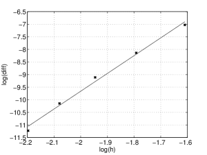
Figure 1. Left: The true solution and estimates given by the three filtering methods. Right: The convergence of $\lim_{k\to\infty}\mathbb{E}\!\left(\left|\!\left|Q\tilde{x}_{k}-\hat{x}_{k}\right|\!\right|_{\mathcal{X}}^{2}\right)$ as $h_{c}\to 0$ is shown with the x-markers. The solid line is a fitted regression line. The plot is in logarithmic scale.

6. Conclusions and remarks

When the system at hand is infinite dimensional (or its dimension is very large), one needs to make some finite (or lower) dimensional approximation of the system in order to be able to actually compute something. For what comes to the Gaussian state estimation problem, the spatial discretization introduces a bias in the Kalman filter but the result can be improved by taking that error into account when determining the Kalman gain.

In this paper, we derived the optimal one-step state estimator $\tilde{x}_{k}$ for an infinite dimensional system that takes values in a pre-defined finite dimensional subspace $\Pi_{s}\mathcal{X}$ of the system’s state space $\mathcal{X}$. The presented method also gives an operator $Q_{k}$ that gives $\mathbb{E}\!\left(x_{k}|\tilde{x}_{k}\right)=Q_{k}\tilde{x}_{k}$. This operator can be used as a sort of post-processor of the obtained state estimate.

Sections 3 and 4 were devoted to finding a bound for the error caused by the discretization. The error measure is the $L^{2}(\Omega,\mathcal{X})$-distance between the reduced-order state estimate $Q_{k}\tilde{x}_{k}$ and the full state Kalman filter estimate $\hat{x}_{k}$, that is, $\mathbb{E}\!\left(\left|\!\left|Q_{k}\tilde{x}_{k}-\hat{x}_{k}\right|\!\right|_{\mathcal{X}}^{2}\right)$. It was found that this distance converges to zero as the approximation abilities of the projection $\Pi_{s}$ improve.

A numerical example on temporally discretized 1D wave equation was presented in Section 5. It was noted that the presented method worked well even with fairly low level of discretization. The spatial discretization was done using piecewise linear hat functions whose approximating properties were noted to converge with rate $\mathcal{O}(h)$ when the discretization is refined. By Theorem 4.1 this would imply convergence rate $\mathbb{E}\!\left(\left|\!\left|Q_{k}\tilde{x}_{k}-\hat{x}_{k}\right|\!\right|_{\mathcal{X}}^{2}\right)=\mathcal{O}(h^{2})$ for the reduced-order state estimate. However, numerical simulations showed that this convergence was actually of order $\mathcal{O}(h^{7})$ in the example case.

6.1. On practical implementation

Even though all the computations needed for the update of the state estimate are carried out in the finite dimensional subspace $\Pi_{s}\mathcal{X}$ in the presented method, the offline computations needed for determining the Kalman gains $K_{k}$ and the operators $Q_{k}$ are still formally carried out in the infinite dimensional $\mathcal{X}$. In practice, there are very few cases where this can be done analytically, and even then it is hardly worth the effort. A practical approach is proposed in the example, namely introducing two computational meshes for the problem at hand — a fine mesh and a coarse mesh. The fine mesh discretization is then regarded as the true system and $K_{k}$ and $Q_{k}$ are computed using this discretization. This mesh should be as fine as reasonably possible. The online state estimation is then carried out in the coarse mesh. Of course, the criterion for this mesh is that the time evolution of the state estimator has to be solvable with the available computing power in time before the next measurement arrives.

In practical implementation of the presented method, one weak point is the computation of $Q_{k}$ which in theory requires computation of the (pseudo)inverse of the $n\times n$ matrix $\tilde{S}_{k}$, see (18). As noted in Remark 2.2, when $\tilde{S}_{k}$ is not invertible then $Q_{k}=\Pi^{*}+(I-\Pi_{s})V_{k}\tilde{S}_{k}^{+}$. This equation for $Q_{k}$ could also be used if the pseudoinverse is not computed accurately, but by using some approximative or regularizing scheme. Then the part that $Q_{k}$ maps to $\Pi_{s}\mathcal{X}$ is readily taken care of and from $V_{k}\tilde{S}_{k}^{+}$ one can compute an approximation to a couple of the most important dimensions in the null space of $\Pi$.

We also remark that there is no guarantee that $Q_{k}$ and $K_{k}$ would converge. Further, even if they do converge, there are no algebraic equations for obtaining the limits directly. Thus, the only way to obtain them is to iterate the recursive equation sufficiently many times. However, consider the case that we are given $\Pi x_{k}$ and we want to recover $x_{k}$. Then (assuming $\mathbb{E}\!\left(x_{k}\right)=0$) the optimal solution is given by $\mathbb{E}\!\left(x_{k}|\Pi x_{k}\right)=:\widehat{Q}_{k}\Pi x_{k}$ where

$$\widehat{Q}_{k}=\Pi^{*}+(I-\Pi_{s})S_{k}\Pi^{*}(\Pi S_{k}\Pi^{*})^{+}$$

where $S_{k}=\textup{Cov}\left[x_{k},x_{k}\right]$ is given by (15). Then we have $x_{k}=\widehat{Q}_{k}\Pi x_{k}+v_{k}$ where $v_{k}\sim N(0,\widehat{V}_{k})$ where

$$\widehat{V}_{k}=(I-\Pi_{s})S_{k}(I-\Pi_{s})^{*}-(I-\Pi_{s})S_{k}\Pi^{*}(\Pi S_{k}\Pi^{*})^{+}\Pi S_{k}(I-\Pi_{s})^{*}.$$

Now $S_{k}$ converges and the limit $S_{\infty}$ can be obtained as the solution of the Lyapunov equation $S_{\infty}=AS_{\infty}A^{*}+BUB^{*}$. Of course, the error $v_{k}$ is correlated but making the (false) assumption that it is not, leads to an approximate reduced order error covariance (in converged form)

$$\begin{cases}\tilde{P}=\Pi A\widehat{Q}_{\infty}P\widehat{Q}_{\infty}^{*}A^{*}\Pi^{*}+\Pi BUB^{*}\Pi^{*}+\Pi A\widehat{V}_{\infty}A^{*}\Pi^{*},\\ P=\tilde{P}-\tilde{P}\widehat{Q}_{\infty}^{*}C^{*}(C\widehat{Q}_{\infty}\tilde{P}\widehat{Q}_{\infty}^{*}C^{*}+R)^{-1}C\widehat{Q}_{\infty}\tilde{P}.\end{cases}$$

It was found that using this approximative state estimate worked reasonably well in the presented example. With the parameters on the left in Table 1, the error $\left|\!\left|\widehat{Q}_{\infty}\tilde{x}_{k}-x_{k}\right|\!\right|_{\mathcal{X}}^{2}$ was in average over 500 simulations .6148 for the position variable and .8179 for the velocity variable (cf. the right panel of Table 1).

6.2. Further work

Let us end the paper by briefly discussing topics that would require further work. An immediate question is whether a similar result can be obtained for the Kalman–Bucy filter, that is, for continuous time systems. Here the discrete time systems were studied for technical convenience but, in principle, there should not be any reasons why it couldn’t be done. For example the results of [2], [3] and [7] were obtained in the continuous time setting. In particular [7] might give useful tools for treating this problem.

The dual problem to the Gaussian state estimation problem is the optimal control problem for linear systems with quadratic cost functions. A natural question is whether the results of this paper can be translated to that problem. For example Mohammadi et al. use truncated eigenbasis approach to approximately solve the algebraic Riccati equation arising from optimal control of a diffusion-convection-reaction in [16].

One topic that was not given much attention in this paper is the optimality of the assumptions on the system. It is well known that the classical Kalman filter might work just fine even though the underlying system is not stable. We, on the other hand, used many times the input stability of the system, i.e., the state covariance is uniformly bounded by some trace class operator $S_{k}\leq S$. Also, we had to state as an assumption that the full state Kalman filter is exponentially stable, that is, $\sigma(A-\hat{K}CA)\subset B(0,\rho)$ for some $\rho<1$. Relaxing this assumption would be desirable since for example strong (that is, asymptotical) stability of the full state filter is proved in [10: Theorem 4.2] — although under a controllability assumption that would exclude finite dimensional control.

Acknowledgements

The author has been supported by the Finnish Graduate School in Engineering Mechanics. The author thanks Dr. Jarmo Malinen for valuable comments on the manuscript.

Appendix A Auxiliary results

Lemma A.1.

Define the operator ${\bf L}\in\mathcal{L}(\mathcal{L}^{*}(\mathcal{X}))$ by

$${\bf L}W:=W-(A-K^{(F)}CA)W(A-K^{(F)}CA)^{*}$$

where $\sigma(A-K^{(F)}CA)\subset B(0,\rho)$ for $\rho<1$. This operator has the following properties:

• ${\bf L}$ is boundedly invertible.

• If ${\bf L}W=X$, then $X\geq 0$ implies $W\geq 0$.

• There exists a constant $L>0$ s.t. $\textup{tr}({\bf L}^{-1}X)\leq L\textup{tr}(X)$ for all positive definite trace class operators $X\in\mathcal{L}^{*}(\mathcal{X})$. Denote by $L$ the smallest possible constant. Denote $L_{0}:=\sum_{j=0}^{\infty}\left|\!\left|(A-K^{(F)}CA)^{2j}\right|\!\right|_{\mathcal{L}(\mathcal{X})}$. We have $L\leq L_{0}<\infty$.

Define also $\tilde{\bf L}W:=W-(A-K_{\infty}CA)W(A-K_{\infty}CA)^{*}$ where $K_{\infty}$ is the converged gain of the reduced order filter (if it converges) and denote by $\tilde{L}$ the corresponding trace bound for $\tilde{\bf L}^{-1}$.

Proof.

(i): The inverse of ${\bf L}$ is given by

(29) $${\bf L}^{-1}X=\sum_{j=0}^{\infty}(A-K^{(F)}CA)^{j}X((A-K^{(F)}CA)^{*})^{j}.$$

By Gelfand’s formula (see [13: Theorem 7.5-5]), the sum converges in operator topology because $\sigma(A-K^{(F)}CA)\subset B(0,\rho)$ for some $\rho<1$.

(ii): Assume that $X\in\mathcal{L}^{*}(\mathcal{X})$ is positive semidefinite. From (29) it is easy to see that ${\bf L}^{-1}X$ is positive semidefinite. Clearly also if $X$ is negative semidefinite then $W$ is negative semidefinite.

(iii): If $X\in\mathcal{L}^{*}(\mathcal{X})$ is a positive definite trace class operator and $T\in\mathcal{L}(\mathcal{X})$ then $\textup{tr}(TXT^{*})\leq\left|\!\left|T\right|\!\right|_{\mathcal{L}(\mathcal{X})}^{2}\textup{tr}(X)$. This together with (29) imply (iii). ∎

If ${\bf L}W=X_{+}-X_{-}$ where $X_{+},X_{-}\geq 0$ then $W=W_{+}-W_{-}$ where ${\bf L}W_{\pm}=X_{\pm}$ and $W_{+},W_{-}\geq 0$. Of course $\textup{tr}(W)\leq\textup{tr}(W_{+})\leq L\textup{tr}(X_{+})$. Thus, if the right hand side can be represented as a sum of a positive definite and a negative definite part, then only the positive definite part needs to be taken into account when computing an upper bound for the trace of the solution.

Lemma A.2.

The perturbation $\Delta P$ in the proof of Theorem 4.1 satisfies

$$\Delta P=(A-K^{(F)}CA)\Delta P(A-K^{(F)}CA)^{*}+E_{1}+E_{2}+h_{1}(\Delta P)+h_{2}(\Delta P)$$

(30) $$={\bf L}^{-1}\left(E_{1}+E_{2}+h_{1}(\Delta P)+h_{2}(\Delta P)\right)$$

where

$$E_{1}=(I-K^{(F)}C)AMA^{*}(I-K^{(F)}C)^{*},$$

$$E_{2}=-(I-K^{(F)}C)AMA^{*}C^{*}\left(C(\tilde{P}^{(F)}+AMA^{*})C^{*}+R\right)^{-1}CAMA^{*}(I-K^{(F)}C)^{*}$$

$$+K^{(F)}CAMA^{*}C^{*}\left(C(\tilde{P}^{(F)}+AMA^{*})C^{*}+R\right)^{-1}CAMA^{*}C^{*}K^{(F)*},$$

$$h_{1}(\Delta P)=\Delta KCA\Delta P(A-K^{(F)}CA)^{*}+(A-K^{(F)}CA)\Delta P(\Delta KCA)^{*}+\Delta KCA\Delta P(\Delta KCA)^{*}$$

where $\Delta K=K^{(F)}-K^{(b)}$, and

$$h_{2}(\Delta P)= -(A-K^{(b)}CA)\Delta PA^{*}C^{*}\!\left(C(\tilde{P}^{(F)}\!+AMA^{*}\!+A\Delta PA^{*})C^{*}\!+R\right)^{-1}\!\times$$

$$\qquad\qquad\times CA\Delta P(A-K^{(b)}CA)^{*}.$$

Alternatively, the equation (30) can be written as

(31) $$\Delta P=(A-K^{(b)}CA)\Delta P(A-K^{(b)}CA)^{*}+E_{1}+E_{2}+h_{2}(\Delta P).$$

The perturbation of the Kalman gain is given by

$$\Delta K= \left((\tilde{P}^{(F)}+AMA^{*})C^{*}\left(C(\tilde{P}^{(F)}+AMA^{*})C^{*}+R\right)^{-1}C-I\right)\times$$

$$\qquad\qquad\times AMA^{*}C^{*}(C\tilde{P}^{(F)}C^{*}+R)^{-1}.$$

For a proof, see [23: Lemma 2.1]. There everything is finite-dimensional but the proof of this Lemma is based on just algebraic manipulation and it holds also in the infinite-dimensional setting. Note that the matrix $C(\tilde{P}^{(F)}+M+A\Delta PA^{*})C^{*}+R$ is invertible because $C(\tilde{P}^{(F)}+M+A\Delta PA^{*})C^{*}\geq 0$ and $R>0$. In the proof of [23: Lemma 2.1], some additional assumptions on the perturbations is needed to guarantee the invertibility of the corresponding matrix (denoted by $\tilde{C}$ there). To get (31), note that

$$h_{1}(\Delta P)=(A-K^{(b)}CA)\Delta P(A-K^{(b)}CA)^{*}-(A-K^{(F)}CA)\Delta P(A-K^{(F)}CA)^{*}.$$

For the last part, see in particular [23: Eq. (A.8)].

References

Bensoussan [1971] Bensoussan,
A. (1971). Filtrage Optimal des Systèmes linéaires,
Dunod, Paris.
Bernstein and Hyland [1985]
Bernstein, D. and Hyland, D. (1985). “The optimal projection
equations for reduced-order state estimation,” Transactions on Automatic
control 30, 583–585.
Bernstein and Hyland [1986]
Bernstein, D. and Hyland, D. (1986). “The optimal projection
equations for finite-dimensional fixed-order dynamic compensation of
infinite-dimensional systems,” SIAM Journal on Control and Optimization
24, 122–151.
Bogachev [1998]
Bogachev, V. (1998). Gaussian Measures, American Mathematical Society,
Mathematical Surveys and Monographs, 62.
Da Prato and Zabczyk [1979]
Da Prato, G. and Zabczyk, J. (1979). Stochastic Equations in
Infinite Dimensions, Encyclopedia of Mathematics and its Applications, 44, Cambridge University Press.
De Souza [1989]
De Souza, C. (1989). “On stabilizing properties of solutions
of the Riccati difference equation,” Transactions on Automatic control
34, 1313–1316.
Germani et al. [1988]
Germani, A., Jetto, L., and Piccioni, M. (1988). “Galerkin
approximation for optimal linear filtering of infinite-dimensional linear
systems,” SIAM Journal on Control and Optimization 26, 1287–1305.
Hager and Horowitz [1976]
Hager, W. W. and Horowitz, L. L. (1976). “Convergence and
stability properties of the discrete Riccati operator equation and the
associated optimal control and filtering problems,” SIAM Journal on Control
and Optimization 14, 295–312.
Hiltunen et al. [2011]
Hiltunen, P., Särkkä, S., Nissilä, I., Lajunen, A., and Lampinen, J.
(2011). “State space regularization in the nonstationary
inverse problem for diffuse optical tomography,” Inverse Problems
27.
Horowitz [1974]
Horowitz, L. L. (1974). Optimal Filtering of Gyroscopic Noise, PhD.
thesis, Massachusetts Institute of Technology.
Huttunen and Pikkarainen [2007]
Huttunen, J. and Pikkarainen, H. (2007). “Discretization error
in dynamical inverse problems: one-dimensional model case,” Journal of
Inverse and Ill-posed Problems 15, 365–386.
Kalman [1960]
Kalman, R. (1960). “A new approach to linear filtering and
prediction problems,” Journal of Basic Engineering 82, 35–45.
Kreyszig [1989]
Kreyszig, E. (1989). Introductory Functional Analysis with
Applications, Wiley & Sons.
Krug [1991]
Krug, P. (1991). “The conditional expectation as estimator of
normally distributed random variables with values in infinitely dimensional
Banach spaces,” Journal of Multivariate Analysis 38, 1–14.
Larsson and Thomée [2005]
Larsson, S. and Thomée, V. (2005). Partial Differential Equations
with Numerical Methods, Texts in Applied Mathematics 45, Springer-Verlag.
Mohammadi et al. [2012]
Mohammadi, L., Aksikas, I., Dubljevic, S., and Forbes, J. (2012).
“LQ-boundary control of a diffusion-convection-reaction system,”
International Journal of Control 2, 171–181.
Pikkarainen [2006]
Pikkarainen, H. (2006). “State estimation approach to
nonstationary inverse problems: discretization error and filtering problem,”
Inverse Problems 22, 365–379.
Seppänen et al. [2001]
Seppänen, A., Vauhkonen, M., Somersalo, E., and Kaipio, J. (2001).
“State space models in process tomography — approximation of state
noise covariance,” Inverse Problems in Engineering 9, 561–585.
Simon [2007]
Simon, D. (2007). “Reduced order kalman filtering without
model reduction,” Control and Intelligent Systems 35, 169–174.
Sims [1982]
Sims, C. (1982). “Reduced-order modelling and filtering,”
Control and Dynamic Systems 18, 55–103.
Solin and Särkkä [2013]
Solin, A. and Särkkä, S. (2013). “Infinite-dimensional
Bayesian filtering for detection of quasiperiodic phenomena in
spatiotemporal data,” Physical Review E 88, 052909.
Stubberud and Wismer [1970]
Stubberud, A. and Wismer, D. (1970). “Suboptimal Kalman
filter techniques,” in C. Leondes, ed., “Theory and Applications of
Kalman Filtering,” Advisory Group for Aerospace Research and Development,
105–117.
Sun [1998]
Sun, J. (1998). “Sensitivity analysis of the discrete-time
algebraic Riccati equation,” Linear Algebra and its Applications
275–276, 595–615.