Non-Adiabatic Quantum Dynamics of Grover’s Adiabatic Search Algorithm

Abstract

We study quantum dynamics of Grover’s adiabatic search algorithm with the equivalent two-level system. Its adiabatic and non-adiabatic evolutions are visualized as trajectories of Bloch vectors on a Bloch sphere. We find the change in the non-adiabatic transition probability from exponential decay for short running time to inverse-square decay for long running time. The size dependence of the critical running time is expressed in terms of Lambert $W$ function. The transitionless driving Hamiltonian is obtained to make a quantum state follow the adiabatic path. We demonstrate that a constant Hamiltonian, approximate to the exact time-dependent driving Hamiltonian, can alter the non-adiabatic transition probability from the inverse square decay to the inverse fourth power decay with running time. This may open up a new way of reducing errors in adiabatic quantum computation.

Introduction–

Grover’s quantum search algorithm Grover97 is known to find a marked one out of $N$ entries with the $O(\sqrt{N})$ queries on a quantum computer, otherwise the $O(N)$ queries are needed on a classical computer. While it was initially designed to be implemented on a quantum circuit model, its adiabatic quantum computation version Farhi , called Grover’s adiabatic search algorithm, was also proposed and the equivalence between them was proved Vandam ; Aharonov ; Roland03 .

Much attention has been paid to solving an instantaneous eigenvalue problem of a time-dependent Hamiltonian of an adiabatic quantum algorithm because the minimum gap of a system determines the validity of an adiabatic quantum evolution and thus its computational complexity Messiah ; Farhi . The non-adiabatic transition to other states, i.e., the deviation from the adiabatic evolution, is the main concern in adiabatic quantum computation. To know in detail how the non-adiabatic transition decreases asymptotically with running time, the minimum gap of the instantaneous eigenvalues is not enough, so a time-dependent Schrödinger equation has to be solved.

In this paper, we study quantum dynamics of Grover’s adiabatic search algorithm with an equivalent two-level system to calculate its non-adiabatic transition probability. The adiabatic and non-adiabatic evolutions of a quantum state are represented by trajectories on a Bloch sphere. We show that the non-adiabatic transition probability changes from exponential decay for short running time to inverse square decay for long running time. The dependence of the critical running time on the problem size is written in terms of Lambert $W$ function. Finally, We show that a constant driving Hamiltonian could reduce significantly the non-adiabatic transition probability, which may speed up adiabatic quantum computation.

Hamiltonian of adiabatic search algorithm–

Let us start with introducing the time-dependent Hamiltonian for Grover’s adiabatic search algorithm Roland03 ; Schaller . The adiabatic quantum computation is based on the adiabatic theorem which states that if a time-dependent Hamiltonian changes slowly enough, then an eigenstate of an initial Hamiltonian, an input state, evolves to an eigenstate of a final Hamiltonian, an output state Farhi ; Messiah . Grover’s search algorithm takes the input state as a superposition of all possible states $|{\varphi_{\rm in}}\rangle=\frac{1}{\sqrt{N}}\sum_{i=0}^{N-1}|{i}\rangle$ with $N$ entries. It is the ground state of the initial Hamiltonian $H_{0}=\mathbf{I}-|{\varphi_{\rm in}}\rangle\langle{\varphi_{\rm in}}|=\mathbf{I}-\frac{1}{N}\sum_{i,j}|{i}\rangle\langle{j}|$ where $\mathbf{I}$ is an $N\times N$ identity matrix. Note that $\sum_{i,j}|{i}\rangle\langle{j}|$ is a matrix with all entries 1 whose eigenvalues are 0 ($N-1$ multiples) and $N$ Horn . The output or target state $|{w}\rangle$ to find is the ground state of the final (or problem) Hamiltonian $H_{p}=\mathbf{I}-|{w}\rangle\langle{w}|$. The slow change from the initial to final Hamiltonians can be done as $H(t)=f(s)H_{0}+g(s)H_{p}$ where $s\equiv t/T$ is the dimensionless (or macroscopic) time Messiah ; Betz , $T$ is the running time acting as an adiabatic parameter, and a turn-off function $f(s)$ and turn-on function $g(s)$ satisfy $f(0)=g(1)=1$ and $f(1)=g(0)=0$. The simplest choice of $f$ and $g$ is to interpolate $H_{0}$ and $H_{p}$ linearly, i.e., $f(s)=1-s$ and $g(s)=s$.

Instantaneous eigenvalues and eigenstates–

Grover’s search algorithm is understood as a rotation from the input state $|{\varphi_{\rm in}}\rangle$ to the target state $|{w}\rangle$. This implies it is essentially a two-dimensional problem formed by two linearly-independent vectors $|{\varphi_{\rm in}}\rangle$ and $|{w}\rangle$. While in quantum circuit model the full rotation is done by $O(\sqrt{N})$ successive finite rotations, it is done by a continuous rotation in adiabatic quantum computation. The two vectors $|{w}\rangle$ and $|{\varphi_{\rm in}}\rangle$ are linearly independent but not orthogonal. An orthonormal basis is easily constructed from the matrix representation of $\mathbf{I}-H(s)=f(s)|{\varphi_{\rm in}}\rangle\langle{\varphi_{\rm in}}|+g(s)|{w}\rangle\langle{w}|$ whose only the $w$-th diagonal element is different. Thus, the time-dependent Hamiltonian for Grover’s adiabatic search algorithm is represented with the orthonormal basis $\{|{w}\rangle,|{w_{\perp}}\rangle\}$ as

$$H(s)=\mathbf{I}-\frac{f}{N}\left[\begin{array}[]{cc}1+N\frac{g}{f}&\sqrt{N-1}\\[10.0pt] \sqrt{N-1}&N-1\end{array}\right]\,,$$ (3)

where $|{w_{\perp}}\rangle=\frac{1}{\sqrt{N-1}}\sum_{i\neq w}^{N}|{i}\rangle\,.$ Hamiltonian (3) is written in convenient form as

$$H(s)=\frac{(f+g)}{2}\,\mathbf{I}-\frac{1}{2N}\left[\begin{array}[]{rr}Z(s)&X(s)\\[10.0pt] X(s)&-Z(s)\end{array}\right]\,,$$ (6)

where $Z(s)\equiv 2f+N(g-f)$ and $X(s)\equiv 2f\sqrt{N-1}$. Since the first term in Eq. (6) is not relevant to dynamics, it will be dropped. The Hamiltonian is written as

$$H(s)=-\frac{\hbar\omega(s)}{2}\left[\begin{array}[]{rr}\cos\theta(s)&\sin\theta(s)\\[10.0pt] \sin\theta(s)&-\cos\theta(s)\end{array}\right]\,,$$ (9)

where the gap between the ground and excited states is given by $\hbar\omega(s)\equiv\frac{1}{N}\sqrt{Z^{2}+X^{2}}=\sqrt{(f-g)^{2}+\frac{4}{N}fg}\,$. Here mixing angle $\theta$ is defined by $\tan\theta(s)\equiv X(s)/Z(s)$. While a different choice of $f$ and $g$ gives rise to a different energy gap, hereafter we consider only a linear interpolation case. Hereafter we set $\hbar=1$.

As in a textbook of quantum mechanics, the instantaneous eigenstates of $H(s)|{e_{\pm}(s)}\rangle=e_{\pm}(s)|{e_{\pm}(s)}\rangle$ read

$$|{e_{-}(s)}\rangle=\left[\begin{array}[]{cc}\cos\tfrac{\theta}{2}\\[10.0pt] \sin\tfrac{\theta}{2}\end{array}\right]\,,\quad|{e_{+}(s)}\rangle=\left[\begin{array}[]{rr}-\sin\tfrac{\theta}{2}\\[10.0pt] \cos\tfrac{\theta}{2}\end{array}\right]\,.$$ (14)

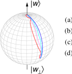
As represented by a Bloch vector in Fig. 1, the input state $|{\varphi_{\rm in}}\rangle=|{e_{-}(0)}\rangle$ is a vector with azimuthal angle $\tan\theta=(2-N)/2\sqrt{N-1}$. The target state $|{w}\rangle=|{e_{-}(1)}\rangle$ points to the north pole. Thus, like the Landau-Zener-Majorana-Stückelberg problem Landau ; Zener ; Majorana ; Stuckelberg , Grover’s adiabatic search algorithm is just a rotation of a single qubit driven by time-dependent Hamiltonian (9).

Figure 1: (color online). Trajectories of a Bloch vector ${\bf r}(t)$ on a Bloch sphere for various running times (a) $T=10$, (b) $T=100$, (c) $T=300$. (d) The blue longitudinal line represents the adiabatic path. Here $N=4$ is set. If $N$ is large, an initial Bloch vector becomes closer to $|{w_{\perp}}\rangle$.

Quantum dynamics of adiabatic search algorithm–

To understand non-adiabatic effects, we solve numerically a time-dependent Schrödinger equation

$$i\hbar\frac{d}{dt}|{\psi(t)}\rangle=H_{T}(t)|{\psi(t)}\rangle\,,$$ (15)

where a time-dependent Hamiltonian $H_{T}(t)$ is given by Eq. (9). As illustrated in Fig. 1, a quantum state $|{\psi(t)}\rangle=\alpha(t)|{w}\rangle+\beta(t)|{w_{\perp}}\rangle$ is visualized by a Bloch vector ${\bf r}(t)\equiv\langle{\psi(t)}|\bm{\sigma}|{\psi(t)}\rangle$ with Pauli matrices $\sigma_{k}$ for $k=x,y,z$. In the adiabatic limit of $T\gg\sqrt{N}$, an evolved quantum state remains in the instantaneous ground state, that is, $|{\psi(t)}\rangle\simeq|{e_{-}(t)}\rangle$ up to the dynamical and geometric phase factors. So, the Bloch vector ${\bf r}_{\rm ad}(s)=\langle{e_{-}(s)}|\bm{\sigma}|{e_{-}(s)}\rangle$ travels to the north pole along the longitude line on a Bloch sphere.

Figure 2: (color online). Transition probability $P(s)$ of being in an instantaneous eigenstate $|{e_{+}(s)}\rangle$ as a function of $s$ for (a) $T=20$, (b) $T=200$, (c) $T=500$, (d) $T=1000$. Here the system size $N=10$ is taken. $P(s)$ is magnified by $10,300,2000,10000$ times, respectively.

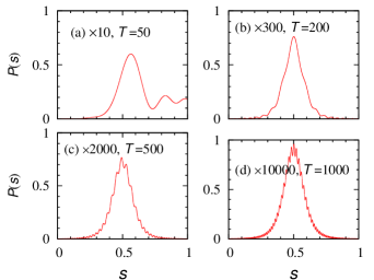
The adiabatic path is a good approximation to the exact evolution if running time $T$ is large enough, that is, the Hamiltonian changes slowly enough. For finite running time $T$, however, a real path deviates from the adiabatic path as illustrated in Fig. 1. To see this in detail, we examine how a quantum state $|{\psi(t)}\rangle$ is deviated from the instantaneous eigenstate $|{e_{-}(t)}\rangle$ as adiabatic parameter $T$ is varied. The evolved state $|{\psi(t)}\rangle$ is written in terms of instantaneous eigenstates as $|{\psi(s)}\rangle=a(s)|{e_{-}(s)}\rangle+b(s)|{e_{+}(s)}\rangle\,$. Fig. 2 plots the transition probability $P(s)=1-|a(s)|^{2}$ of being in an instantaneous ground state $|{e_{+}(s)}\rangle$ for various running time $T$. For short running time $T$, as shown in Fig. 2 (a), the maximum of $P(s)$ does not coincide with the location of the minimum energy gap. As depicted in Figs. 2 (b), (c), and (d), $P(s)$ becomes smaller and more symmetric and reaches at its peak at $s=1/2$ as running time $T$ is increased.

Transition of non-adiabatic transition–

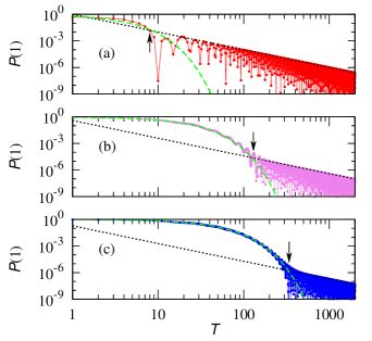
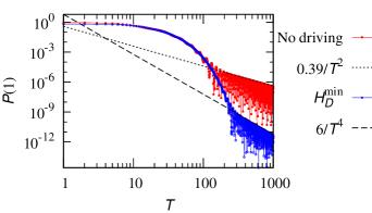
The non-adiabatic transition probability $P(1)$ at $s=1$ indicates the error of adiabatic quantum computation. The asymptotic form of $P(1)$ for the Landau-Zener-Majorana-Stückelberg problem is known to decrease exponentially Landau ; Zener ; Majorana ; Stuckelberg . Suzuki and Okada Suzuki , however, calculated numerically the residual energy, the difference between the energy expectation $E(s)=\langle{\psi(s)}|H(s)|{\psi(s)}\rangle$ and the instantaneous ground energy $e_{-}(s)$, for a modified Landau-Zener-Majorana-Stükelberg problem. They showed the transition of the residual energy from exponential decay only for short running time to the inverse-square decay for long running time. The similar result was obtained by Rezakhani et al. Rezakhani . Note $1/T^{2}$ decay was reported for the simulated annealing system by Santoro et al. Santoro and for adiabatic quantum teleportation by Oh et al. Oh13 . As illustrated in Fig. 3, we calculate numerically the non-adiabatic transition probability $P(1)$ as a function of running time $T$ and find

$$P(1)\sim\begin{cases}\exp\left(-A\,T\right)&\text{for\, $T<T_{c}$}\\[10.0pt] B/{T^{2}}&\text{for\, $T>T_{c}$}\end{cases}\,.$$ (16)

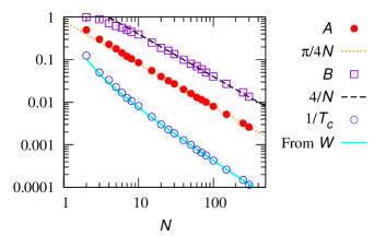
The coefficients $A$, $B$, and the transition time $T_{c}$ depend on the system size $N$, as shown in Fig. 4. The numerical data show $A\sim\pi/4N$ and $B\sim 4/N$. The critical running time $T_{c}$ can be defined by a solution of the transcendental equation $e^{-A\,T}=B/T^{2}$ in Eq. (16). It is given by

$$T_{c}=-\frac{2}{A}W_{-1}\left(-\frac{A\sqrt{B}}{2}\right)\sim\frac{8N}{\pi}W_{-1}\left(-\frac{\pi}{4\sqrt{N^{3}}}\right)\,,$$ (17)

where $W_{-1}$ is the lower branch of the Lambert $W$ function Lambert ; Corless .

Figure 3: (color online). Log-log plots of the non-adiabatic transition probability $P$ as function of running time $T$ for (a) $N=$ 2, (b) $N=10$, and (c) $N=20$. The green dashed line is $\exp(-AT)$ and the black dotted line is $B/T^{2}$. The arrows indicate the critical running time $T_{c}$.

Figure 4: (color online). Coefficients $A$ and $B$ in Eq. (16), and $1/T_{c}$ as a function of the system size $N$. The cyan solid line is a plot with Eq. (17).

Transitionless driving–

When the time-dependent Schrödinger equation is transformed to the adiabatic frame, it is clearly seen why the non-adiabatic transition happens. Demirplak and Rice Demirplak , and Berry Berry showed that a time-dependent Hamiltonian $H_{D}(t)$, called the counter or transitionless driving term, in addition to the original time-dependent Hamiltonian makes a quantum state follow the original adiabatic state exactly. The main idea is to make a driving Hamiltonian cancel the non-adiabatic term seen in the adiabatic frame. The driving Hamiltonian $H_{D}(t)$ for Hamiltonian (9) reads

$$H_{D}(t)=i\hbar\,\frac{\partial U^{{\dagger}}(t)}{\partial t}\,U(t)=-\hbar\,\frac{\dot{\theta}}{2}\,\sigma_{y}$$ (18)

where the unitary operator $U(t)$ is composed of instantaneous eigenstates $|{e_{\pm}(t)}\rangle$

$$U(t)=\left[\begin{array}[]{rr}\cos\frac{\theta}{2}&-\sin\frac{\theta}{2}\\[10.0pt] \sin\frac{\theta}{2}&\cos\frac{\theta}{2}\end{array}\right]\,,$$ (21)

and $\dot{\theta}=\frac{d\theta}{ds}\frac{ds}{dt}=\frac{1}{T}\frac{d\theta}{ds}$. Note Pauli operator $\sigma_{y}$ is represented by $\sigma_{y}=-i|{w}\rangle\langle{w_{\perp}}|+i|{w_{\perp}}\rangle\langle{w}|$. For linear interpolation, one has $\dot{\theta}(t)=2\frac{\sqrt{N-1}}{NT}\left[(1-2s)^{2}+\frac{4}{N}(1-s)s\right]^{-1}$. As expected, the driving Hamiltonian goes to zero in the adiabatic limit, $T\gg 1$.

While the driving Hamiltonian $H_{D}(t)$ makes a quantum state evolve exactly along the longitudinal line (adiabatic path) regardless of $T$, it seems to be difficult to control the strength $\dot{\theta}$ even in linear interpolation case. So, we investigate whether an approximate but constant driving Hamiltonian, instead of the exact time-dependent driving Hamiltonian (18), could reduce some errors. We consider two constant driving Hamiltonians which are the minimum and maximum values of $H_{D}$, respectively

$$H_{D}^{\min}=-\frac{\hbar\sqrt{N-1}}{NT}\,\sigma_{y}\,,\;\;H_{D}^{\max}=-\frac{\hbar\sqrt{N-1}}{T}\,\sigma_{y}\,.$$ (22)

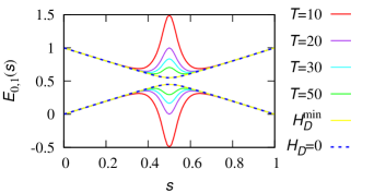
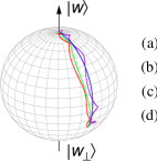
Fig. 5 shows how the instantaneous eigenvalues change when the driving Hamiltonian $H_{D}(s)$ is added to $H(s)$. The role of $H_{D}$ is to make the gap at the avoided crossing wider. While the approximate driving Hamiltonian $H_{D}^{\rm min}$ seems to make a very little change in adiabatic energy levels and the trajectory as shown in Fig. 6, it produces drastic change in the non-adiabatic transition probability for long running time, from $O(1/T^{2})$ to $O(1/T^{4})$ as depicted in Fig. 7. Let take a close look at it in connection with the adiabatic condition

$$T\gg\frac{\max_{s}|\langle{e_{+}(s)}|\frac{dH}{ds}|{e_{-}(s)}\rangle|}{\min_{s}\Delta E(s)^{2}}\,,$$ (23)

where $\Delta E$ is the energy gap. For two Hamiltonians $H(s)$ and $H(s)+H_{\min}^{D}$ with $T=10$, while the numerators in Eq. (23) are same, the denominators change slightly, to be more specific, from $0.01$ to $0.010396$. Although the right-hand side of the inequality (23) changes very little, $P(1)$ for long running time changes from the inverse square to fourth power decays. Note that $H_{D}^{\rm min}$ also reduces $P(1)$ for short running time.

Figure 5: (color online). Instantaneous eigenvalues $E_{0,1}(s)$ of $H(s)+H_{D}(s)$ as a function of $s$ for $T=10,20,30,50$, $H_{D}^{\rm min}$ at $T=10$, and $H_{D}=0$. The size of the system is $N=100$.

Figure 6: (color online). Trajectories of Bloch vectors on a Bloch sphere when the quantum evolution is driven (a) by adiabatically or exactly $H_{D}(t)$, (b) by $H_{D}^{\min}$, (c) by $H_{D}^{\max}$, and (d) without driving. Here $N=4$ and $T=10$ are taken.

Figure 7: (color online). Non-adiabatic transition probability $P(1)$ as a function of running time $T$ with $H_{D}^{\min}$ (blue) and without driving Hamiltonian (red). Here $N=10$ is taken.

Conclusion–

We studied quantum dynamics of Grover’s adiabatic search algorithm as a time-dependent two-level system. The transition from the non-adiabatic and adiabatic quantum evolutions were visualized by changes in trajectories of Bloch vectors on a Bloch sphere. We found a drastic change in the non-adiabatic transition probability from well-known exponential decay for short running time to the inverse-square decay for longer running time. The dependence of the critical running time on the problem size is obtained with Lambert $W$ function. We showed an approximate but constant driving Hamiltonian could reduce the non-adiabatic transition probability significantly which becomes the inverse fourth power decay for long running time. It would be interesting to see whether the results obtained in this paper could be applied to other quantum system, for example, a quantum Ising model Campo , or quantum optimization problems Boixo . While our results was obtained by numerical calculations, it would be interesting to seek an exact analytic solution.

References

- (1) Lov K. Grover, Phys. Rev. Lett. , 79, 325 (1997).
- (2) E. Farhi, J. Goldstone, S. Gutmann, J. Lapan, A. Lundgren, and D. Preda, Science 292, 472 (2001).
- (3) W. van Dam, M. Mosca, and U. Vazirani, Proceedings of the 42nd Annual Symposium on Foundations of Computer Science, p. 279-287 (2001).
- (4) D. Aharonov, W. Van Dam, J. KEPME, Z. Landau, S. Lloyd, and O. Regev, SIAM J. Comput. 37, 166 (2007).
- (5) J. Roland and N. J. Cerf, Phys. Rev. A 68, 062311 (2003); ibid, 062312 (2003).
- (6) A. Messiah, Quantum Mechanics (North-Holland, Amsterdam, 1963).
- (7) G. Schaller, S. Mostame, R. Schützhold, Phys. Rev. A 73, 062307 (2006).
- (8) R. A. Horn and C. R. Johnson, Matrix Analysis (Cambridge Univ. Press, Cambridge, 1990), p. 39.
- (9) V. Betz and S. Teufel, in Lect. Notes Phys. 690, 19 (2006).
- (10) L. D. Landau, Physics of the Soviet Union 2, 46 (1932).
- (11) C. M. Zener, Proc. R. Soc. London Ser. A 137, 696 (1932).
- (12) E. Majorana, Nuovo Cimento 9, 43 (1932).
- (13) E. C. G. Stückelberg, Helv. Phys. Acta 5, 369 (1932).
- (14) S. Suzuki and M. Okada, in Lect. Notes Phys. 679, 207 (2005).
- (15) A. T. Rezakhani, A. K. Pimachev, and D. A. Lidar Phys. Rev. A 82, 052305 (2010).
- (16) G. E. Santoro, R. Martoňák, E. Tosatti, and R. Car, Science 295, 2427 (2002).
- (17) S. Oh, Y.-P. Shim, J. Fei, M. Friesen, and X. Hu, Phys. Rev. A 87, 022332 (2013).
- (18) J. H. Lambert, Acta Helvetica, Physico-mathematico-anatomico-13botanico-medica 3, 128 (1758).
- (19) R. M. Corless, G. H. Gonnet, D. E. G. Hare, D. J. Jeffrey, and D. E. Knuth, Adv. in Comp. Math., 5 329 (1996).
- (20) M. Demirplak and S. A. Rice, J. Phys. Chem. A 107, 9937 (2003).
- (21) M. V. Berry, J. Phys. A: Math. Theor. 42, 365303 (2009).
- (22) A. del Campo, M. M. Rams, and W. H. Zurek, Phys. Rev. Lett. 109, 115703 (2012).
- (23) S. Boixo, T. Albash, F. M. Spedalieri, N. Chancellor, and D. A. Lidar, Nat. Commun. 4, 3067 (2013).