Absorption at the dust sublimation radius and the dichotomy between X-ray and optical classification in the Seyfert galaxy H0557-385

Abstract

In this work, the analysis of multi-epoch (1995-2010) X-ray observations of the Seyfert 1 galaxy H0557-385 is presented. The wealth of data presented in this analysis show that the source exhibits dramatic spectral variability, from a typical unabsorbed Seyfert 1 type spectrum to a Compton-thin absorbed state, on time scales of $\sim$ 5 years. This extreme change in spectral shape can be attributed to variations in the column density and covering fraction of a neutral absorbing medium attenuating the emission from the central continuum source. Evidence for Compton reflection of the intrinsic nuclear emission is present in each of the spectra, though this feature is most prominent in the low-state spectra, where the associated Fe emission line complex is clearly visible. In addition to the variable absorbing medium, a warm absorber component has been detected in each spectral state. Optical spectroscopy concurrent with the 2010 XMM-Newton observation campaign have detected the presence of broad optical emission lines during an X-ray absorption event. From the analysis of both X-ray and optical spectroscopic data, it has been inferred that the X-ray spectral variability is a result of obscuration of the central emission region by a clumpy absorber covering $\geq$ 80 per cent of the source with an average column density of N${}_{\text{H}}$ $\sim$ 7$\times$10²³ cm^-2, and which is located outside the broad line region at a distance from the central source consistent with the dust sublimation radius of the AGN.

1 Introduction

This work documents the X-ray and optical spectral analysis of the extreme “changing-look” Seyfert 1 active galactic nucleus (AGN) H0557-385. AGN that exhibit significant X-ray absorption variability have been the focus of intensive research efforts in recent years, since the interpretation of X-ray absorption variability patterns allow the innermost regions of such objects to be studied. In some cases, where the data permitted, the X-ray absorbing medium has been inferred to exist on scales coincident with the optical Broad Line Region (BLR, e.g. Risaliti et al., 2007; Bianchi et al., 2009; Sanfrutos et al., 2013), which is often characterised by short time scale (days/weeks) variability. On the other hand, long time scale (months/years) spectral variations have been associated with absorption by material present in the circumnuclear torus (e.g. Piconcelli et al., 2007; Rivers, Markowitz & Rothschild, 2011; Miniutti et al., 2014), first inferred to exist as the main component of the Unification Model for AGN (Antonucci, 1993; Urry & Padovani, 1995), and eventually spatially resolved via interferometric mid-infrared observations (e.g. NGC 1068, Jaffe et al., 2004).

In order to fully explain the observed properties of AGN, theoretical considerations have shown that the circumnuclear torus is required to consist of a distribution of discrete, or clumpy, clouds at distances from the supermassive black hole (SMBH) of not more than a few pc (Krolik & Begelman, 1988; Elitzur & Shlosman, 2006; Nenkova et al., 2008a, b). Observational evidence in favour of a clumpy toroidal absorber has been obtained via interferometry in the 8 - 13 $\mu$m range in the case of the Circinus Galaxy (Tristram et al., 2007). In addition to the associated obscuration effects, a clumpy circumnuclear torus would imply that the Seyfert 1/2 dichotomy is not only dependent on the torus orientation angle with respect to the observer, but is also dependent on the probability of the observers line of sight (LOS) intercepting a toroidal cloud. Therefore it would be expected that, assuming a clumpy torus, the probability of directly observing the AGN continuum source would always be finite (Elitzur, 2008, 2012).

H0557-385 (z=0.03387) was originally identified as a Seyfert 1 AGN by Fairall, McHardy & Pye (1982). An early analysis into the nature of this source was based on data obtained by ASCA, and was presented by Turner, Netzer & George (1996), where the authors report the presence of continuum absorption below 2 keV. Similar absorption features were detected in subsequent XMM-Newton observations presented by Ashton et al. (2006, hereafter A06), where the spectra suggested that line of sight absorption was present in two distinct ionization phases. Here a phase is defined as gas at a particular column density and ionisation parameter. A06 also report the presence of neutral absorption (N${}_{\text{H}}$ = 1.2$\times$10²¹ cm^-2) attenuating the primary emission, however the data did not allow the location of this component to be well constrained. Further XMM-Newton observations carried out in 2006 showed a dramatic change in spectral shape, with a decrease in flux by a factor of $\sim$10. Longinotti et al. (2009, hereafter L09) interpret this change in spectral shape as being due to a partial covering of the source by neutral circumnuclear clouds. This paper presents the outcome of an intensive observational campaign that was launched in 2010, which includes XMM-Newton and Swift observations in the X-ray domain, and optical spectroscopy obtained at the 4.1 m Southern Astrophysical Research Telescope (SOAR, Chile). Archival X-ray data are also included in this work. Following from the work of L09, this analysis re-examines the spectral variability in terms of the partial covering scenario, using the multi-epoch observational data to impose constraints on the geometry, location, and composition of the absorbing structures.

This paper is organised as follows: In Section 2, the acquisition of all X-ray and optical data used in this analysis will be documented. Section 3 will outline the theoretical model that has been developed, as well as a statistical investigation of the assumptions made while modelling the spectra. Section 4 will then present the physical interpretations of the spectral results, as well as a discussion of the nature of the absorbing medium in H0557-385. The adopted cosmological parameters are H₀ = 70 km s^-1 Mpc^-1, and $\Lambda$ = 0.73.

2 Observations and Data reduction

2.1 X-ray Observations

Table 1: Observation log of H0557-385. For observations 1-9, the fluxes have been measured by applying the best fit model to each individual data set. For the Swift observations, the flux was measured by fitting a powerlaw to each individual data set.
¹ Effective exposure time, or the net exposure time after all filtering processes have been carried out.

Obs. $\#$	Mission	Obs. Id.	Date	Eff. Exp.1	Flux0.3-2	Flux2-10
			year-month-day	(ks)	10-12 erg cm-2 s-1	10-12 erg cm-2 s-1
1	ASCA	73070000	1995-03-23	37	1.5${}^{+1.0}_{-0.8}$	21.8${}^{+1.5}_{-3}$
2	BeppoSAX	511090031	2001-01-26	19	9.6$\pm$0.9	34.3$\pm$1.6
3	XMM	0109130501	2002-04-04	3	10.3${}^{+0.3}_{-0.5}$	34.4${}^{+0.7}_{-0.8}$
4	XMM	0109131001	2002-09-17	4	10.93${}^{+0.2}_{-0.11}$	42.5$\pm{0.7}$
5	XMM	0404260101	2006-08-11	41	0.43${}^{+0.07}_{-0.02}$	3.48${}^{+0.06}_{-0.2}$
6	XMM	0404260301	2006-11-03	56	0.37${}^{+0.08}_{-0.03}$	3.02${}^{+0.09}_{-0.18}$
7	XMM	0651530201	2010-10-15	21	0.60${}^{+0.02}_{-0.15}$	3.3${}^{+0.1}_{-1.1}$
8	XMM	0651530301	2010-10-19	24	0.56${}^{+0.08}_{-0.09}$	3.0${}^{+0.1}_{-0.3}$
9	XMM	0651530401	2010-10-31	21	0.52${}^{+0.08}_{-0.09}$	2.93${}^{+0.05}_{-0.4}$
Swift Monitoring
		Obs. Id.	Date	Eff. Exp.1	Flux${}_{\text{0.4-2}}$	Flux${}_{\text{2-5}}$
			year-month-day	(ks)	10${}^{\text{-13}}$ erg cm${}^{\text{-2}}$ s${}^{\text{-1}}$	10${}^{\text{-13}}$ erg cm${}^{\text{-2}}$ s${}^{\text{-1}}$
		00090392001	2010-04-03	3.5	4.7${}_{-1.9}^{+1.6}$	6.9${}_{-2.5}^{+2.2}$
		00090392002	2010-04-23	3.4	4.6${}_{-1.6}^{+1.9}$	6.7${}_{-2.4}^{+2.1}$
		00090392003	2010-05-13	3.4	4.6${}_{-1.4}^{+1.2}$	6.6${}_{-2.4}^{+2.2}$
		00090392004	2010-06-02	2.6	4.8${}_{-1.7}^{+1.7}$	7.0${}_{-2.5}^{+2.5}$
		00090392005	2010-06-22	3.4	5.6${}_{-2.1}^{+1.8}$	8.4${}_{-2.8}^{+2.4}$
		00090392006	2010-07-12	4.2	5.1${}_{-1.4}^{+1.6}$	7.7${}_{-1.7}^{+2.1}$
		00090392007	2010-08-01	3.7	3.9${}_{-1.8}^{+1.2}$	5.6${}_{-1.6}^{+1.7}$
		00090392008	2010-08-21	4.1	3.9${}_{-1.4}^{+1.4}$	5.8${}_{-2.0}^{+1.9}$
		00090392009	2010-09-10	2.6	7.1${}_{-2.5}^{+2.2}$	10.3${}_{-4.1}^{+3.6}$
		00090392010	2010-09-14	1.6	6.8${}_{-3.8}^{+3.6}$	9.8${}_{-4.4}^{+4.2}$
		00090392011	2010-09-30	3.4	4.6${}_{-1.8}^{+1.8}$	6.8${}_{-2.8}^{+2.0}$
		00090392012	2010-10-20	3.6	5.6${}_{-2.0}^{+1.7}$	8.2${}_{-2.6}^{+2.6}$
		00090392013	2010-11-09	3.8	5.8${}_{-1.6}^{+1.5}$	8.3${}_{-2.4}^{+3.1}$
		00090392014	2010-11-29	3.8	5.9${}_{-1.4}^{+1.8}$	8.7${}_{-2.1}^{+2.6}$
		00090392015	2010-12-19	2.3	5.5${}_{-1.6}^{+2.2}$	7.8${}_{-2.8}^{+3.2}$
		00090392016	2011-01-08	3.0	4.1${}_{-1.6}^{+2.0}$	6.4${}_{-2.4}^{+2.5}$
		00090392017	2011-01-28	3.6	4.6${}_{-2.0}^{+1.4}$	6.5${}_{-2.4}^{+2.6}$
		00090392018	2011-02-17	3.9	4.4${}_{-1.4}^{+1.6}$	6.5${}_{-1.8}^{+2.2}$
		00090392019	2011-03-09	3.7	5.5${}_{-1.4}^{+2.1}$	8.3${}_{-2.5}^{+2.4}$
		00091016001	2011-06-28	1.6	3.4${}_{-2.4}^{+2.0}$	5.0${}_{-2.7}^{+3.7}$
		00091016002	2011-06-29	2.3	4.3${}_{-1.8}^{+2.0}$	6.2${}_{-2.8}^{+2.6}$
		00091016003	2011-08-11	3.7	3.3${}_{-1.5}^{+1.5}$	4.9${}_{-2.4}^{+2.2}$
		00091016004	2011-09-24	3.2	4.8${}_{-2.0}^{+1.5}$	6.9${}_{-3.2}^{+2.1}$
		00091016005	2011-11-07	2.0	2.8${}_{-2.1}^{+1.7}$	4.0${}_{-2.3}^{+1.9}$
		00091016006	2011-11-10	1.5	4.1${}_{-3.1}^{+2.8}$	5.9${}_{-3.0}^{+3.9}$

To date, there have been seven XMM-Newton (Jansen et al., 2001) observations (see Table 1) of the Seyfert 1 AGN H0557-385 taken between 2002 and 2010. In addition, Table 1 includes BeppoSAX and ASCA observations. Spectral products for both observatories were downloaded from the BeppoSAX archive interface and the Tartarus data base, respectively. The BeppoSAX observations of this source have been presented by Quadrelli et al. (2003) and Dadina (2007). The EPIC pn CCD operated in large window mode for the 2002 observations, and in small window mode for all other observations. Both MOS CCDs operated in small window mode for each observation. The observation data files have been processed using the XMM-Newton science analysis systems (SAS) version 13.0.0, including the latest calibration files available as of June 2013.

Intervals of high background activity were removed by first extracting a light curve in the energy range 10 - 12 keV, and then applying rate thresholds of 0.35 counts s^-1 and 0.4 counts s^-1 for the EPIC MOS and EPIC pn respectively. All observations showed relatively low levels of background contamination, except for Obs. 0404260101, where the event list is a combination of two separate event lists that were generated during the observation (L09).

Data obtained from the EPIC pn camera will be the primary focus of the following analysis, and for this reason, the description of all subsequent data reduction and spectral fitting procedures will refer only to EPIC pn spectra, unless otherwise stated. Circular source and background regions were extracted using pattern 0 - 4. For each of the 2006 and 2010 observations, the 0.3 - 10 keV count rate was below the critical value (small window mode: 25 counts s^-1) for which pile-up occurs, while for the 2002 observations the SAS task epatplot was run to verify that the spectra were not affected by pile-up. Inspection of the light curves for each observation reveals that there is no significant spectral variation on the short time scales over which the observations were carried out, therefore the full time-integrated spectra will be used in the following analysis for each observation.

For all observations RGS spectral products were obtained by running the SAS task rgsproc. However, the signal to noise ratio of the 2006 - 2010 data is so low that no accurate spectral measurements could be made. The RGS data of the 2002 observations have been presented in great detail in a previous analysis of this source (A06). Since a detailed analysis of the warm absorber is out of the scope of this paper, their results will be assumed and quoted when necessary. For these reasons, the RGS data will not be included in the present analysis.

From 2010 April to 2011 November the Swift observatory monitored H0557-385 every 3 - 4 weeks (see Table 1). The data from the X-ray Telescope (XRT, Burrows et al. (2005)) were always acquired in Photon Counting mode. The data were reduced with xrtpipeline 0.12.6, spectral products were extracted with xselect from source and background circular regions of 25 and 35 arcsec of radius, respectively.

2.2 Optical Observations

This source was also observed using the SOAR/Goodman optical spectrograph during the period November 2010 - January 2011. The observations were carried out using the 600 l/mm grating and the 0.8” slit width oriented at the position angle PA = 0^∘. The detector consisted of a Fairchild CCD 2048$\times$2048 pixels with a spatial scale of 0.15”/pixel. This setup provides a spectral resolution of 3.2 Å and a spectral coverage from 4360 Å to 6950 Å, allowing the simultaneous detection of H$\gamma$, H$\beta$, [O iii] $\lambda$5007, and H$\alpha$. The first observation was carried out on 2010 October 17 (UT), consuming a total of 1.7 h; the second on 2010 November 3 (UT), with a total of 2.3 h; and the last on 2011 January 30 (UT), lasting 2 h. The former two visits were nearly simultaneous with XMM-Newton pointings, on 2010 October 15 and 2010 October 31. In all cases, the seeing was  0.8” with no photometric conditions.

The observing procedure consisted of recording three individual science frames of 900 s of integration each, totaling 2700 s on-source. Right before or after, a lamp frame of CuHeAr was obtained for wavelength calibration, followed by the observation of a spectroscopic standard star for flux calibration and deriving instrument response. Flats and bias frames were taken as diurnal calibrations.

The optical data were reduced following standard IRAF procedures, that is, bias subtraction and division by a normalised flat field spectrum. The spectra were then extracted by summing up the signal recorded for the galaxy along the spatial direction. Individual 1D spectra of each night were wavelength calibrated using CuHeAr lamp frames and then combined to obtain a single 1D spectrum. It was then flux calibrated using the spectrum of the standard star LTT 2415, for the observations of October and November, and Hiltner 600 for that of January.

Finally, it was necessary to correct the data for Galactic extinction. Here, a value of E(B-V) = 0.038 was adopted, as determined by Schlafly & Finkbeiner (2011). Figure  1 shows the wavelength and flux calibrated optical spectra taken on the three different dates: 2010-10-17, 2010-11-03, and 2011-01-30. Overall, the agreement in the continuum shape and emission line features is very good. Differences in the continuum level, mostly redward of 5300 Å, can be seen but these are of the order of 10 per cent or less. Considering that the observations were carried out under non-photometric conditions and the slit was not oriented at the parallactic angle, differences in the flux level between the different spectra are expected, and can account for the apparent variability.

Figure 1: Spectra of H0557-385 taken on the three different visits to this source. The observations of 2010 Oct 17 and 2010 Nov 03 were displaced along the vertical direction for displaying purposes.

XMM-Newton’s Optical Monitor (OM) telescope carried out observations of the source simultaneously with the EPIC observations. All OM data has been processed using the standard SAS task omichain. For the 2002 and 2006 observations, the OM was operated with the following optical and UV filters: 5430 (V), 4500 (B), 3440 (U), 2910 (UVW1), 2120 (UVW2), and 2310 (UVM2) Å. For the 2010 observations only the UV filters were used: 3440 (U), 2910 (UVW1), and 2310 (UVM2) Å.

3 Spectral Analysis

The following analysis was carried out using xspec version 12.8.0f (Arnaud, 1996). Errors are quoted throughout at the 90 per cent confidence level ($\Delta\chi^{2}$=2.71) for a single parameter of interest. For each of the following spectral models, a Galactic column density of 4$\times$10²⁰ cm^-2 (Dickey & Lockman, 1990) is applied, and all elemental abundances are set to solar values unless stated otherwise.

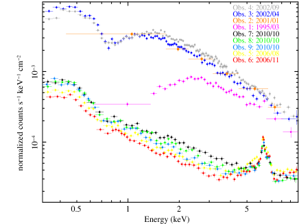
Figure 2: XMM-Newton, ASCA, and BeppoSAX observations of H0557-385.

The X-ray spectra for the nine deepest observations listed in Table 1 are shown in Figure 2. It is noted here that the detailed spectral analysis described in the following sections applies only to Obs. 1 - 9 due to the superior signal to noise ratio of these spectra. The poorer signal to noise ratio of the Swift data render it inappropriate for detailed spectral modelling, and so it will be analysed separately in Section 3.5.

To allow for clearer visual comparison, the spectra in Figure 2 have been divided by the corresponding detector effective area. From inspection of Figure 2, it can be seen that there is dramatic spectral variability observed in this source across the entire 0.3 - 10 keV band. Three main spectral states have been identified in this source; an extreme change in spectral shape occurs between the intermediate- (ASCA 1995), high- (XMM-Newton 2002), and low- (XMM-Newton 2006/2010) state spectra, on a time scale of years. In addition, a less dramatic variation can be seen among the low-state spectra, which occurs on shorter time scales of weeks/months.

The overall strategy for this analysis is as follows; first a model that explains the low-state variability will be defined. Once a robust best-fit for the low-state spectra is established, it will then be used as a global model and extended to all other spectral states. In this way it will be tested if the same physical processes can explain both phases of the variability.

3.1 Determining a Global Spectral Model

The spectral analysis of the low-state spectra began with an analysis of the XMM-Newton Obs. 6 and 7 (see Table 1), since they represent the upper and lower bounds to the observed low-state variability. Since the presence of a two-phase warm absorber in this source is already well documented in the literature (A06 and L09), this component was included in the baseline model that consists of an intrinsic X-ray power law absorbed by a two-phase warm absorber system. The warm absorber is approximated by two zxipcf components (Miller et al., 2007), and the Galactic column density by the tbabs model (Wilms, Allen & McCray, 2000). A Gaussian line at 6.4 keV was added to fit the prominent Fe K$\alpha$ emission clearly visible in the spectra. Following from the conclusion in L09 that the variability between spectral states is due to a neutral partial covering, this component was added (zpcfabs in xspec) such that the intrinsic power law was then absorbed by both ionised and neutral absorption. The spectral indices of the primary emission were assumed to take a common value for both of the spectra (model components that are set to be equal between spectral states in this manner will be referred to throughout as “tied”). The column densities and ionisation parameters of the warm absorbers have also been tied for both epochs (a test of this assumption is presented in Section 3.3). The remaining parameters, which include the normalisation of the power law, and the column density and covering fraction of the neutral absorber, were left free to vary between the states.

This model, which can be considered the basis from which the global model will be built, does not provide a good fit to the data ($\chi_{\nu}^{2}$ = 1.84), as is expected. From inspection of the residuals generated by this fit, it was seen that the model provided a poor fit to the soft X-ray spectrum. In particular, positive residuals were seen to be present around 0.9 keV, which were also observed in L09, where the feature was modelled with a Gaussian line with energy consistent with emission from the Ne ix triplet. Contributions to the 0.5 - 2 keV spectrum is generally expected in AGN from both emission from the photoionised narrow line region (NLR, Bianchi, Guainazzi & Chiaberge, 2006), and gas ionised by stellar activity in the host galaxy (LaMassa, Heckman & Ptak, 2012). To account for this in the CCD spectra, and following the approach presented in Miniutti et al. (2014), the collisionally-ionised gas emission model apec was adopted as a phenomenological description of the residuals in H0557-385. Adding this component improved the fit considerably by $\Delta\chi^{2}$ = 175 for 2 degrees of freedom (DOF) for a plasma temperature of kT $\simeq$ 0.9 keV, with flux F${}^{\text{APEC}}_{\text{0.5\,-\,2}}$ = 5.4 $\pm$ 0.3$\times$10${}^{\text{-14}}$ erg cm${}^{\text{-2}}$ s${}^{\text{-1}}$. Since this component is associated in either case with extended regions, it is expected to remain constant over long time scales, and therefore the normalisation was tied for each epoch. In addition, because this emission is due to activity at larger scales, it is not absorbed by the neutral/ionised components that absorb the primary X-ray emission.

Table 2: Best-fitting parameters for the global fit to each spectral state. The tied components have been set to be equal for each individual data set, but are free to vary for the global fit. The variable components have been left free to vary for each individual data set. Apec plasma temperature in units of keV, norm in units of 10^-5 ph keV^-1 cm^-2 s^-1, pexmon norm in units of 10^-3 ph keV^-1 cm^-2 s^-1, column densities in units of 10²² cm^-2, ionisation parameters, $\xi$, in units of erg cm s^-1, power law norm in units of 10^-2 ph keV^-1 cm^-2 s^-1.
¹ Covering fractions for the fit to the high-state spectra are fixed to one, as it is not expected that this parameter is measureable in these unabsorbed states.
² The unabsorbed 0.3 - 2 keV and 2 - 10 keV luminosities measured using the EPIC best-fit model in units of 10⁴⁴ erg s^-1.

Tied Components
APEC		PEXMON	Warm Absorber1		Warm Absorber2		Power Law	Fit Statistic
kT	Norm	Norm	N${}_{\text{H}}$	Log($\xi$)	N${}_{\text{H}}$	Log($\xi$)	$\Gamma$	$\chi^{2}_{\nu}$
0.853${}^{+0.018}_{-0.02}$	1.94$\pm{0.09}$	2.78$\pm{0.11}$	2.65$\pm{0.04}$	2.11$\pm{0.01}$	0.243$\pm{0.004}$	0.27$\pm{0.01}$	1.978$\pm{0.004}$	1.35
Variable Components
	Obs. $\#$	Power Law	Neutral Absorber		L${}_{0.3-2}^{2}$	L${}_{2-10}^{2}$
		Norm	N${}_{\text{H}}$	C${}_{\text{f}}$
	1	1.01$\pm{0.03}$	2.27$\pm{0.08}$	0.917$\pm{0.013}$	0.5$\pm{0.3}$	0.7$\pm{0.1}$
	3	1.443$\pm{0.015}$	0.089$\pm{0.003}$	11	1.16$\pm{0.06}$	1.03$\pm{0.02}$
	4	1.769$\pm{0.014}$	0.138$\pm{0.003}$	11	1.417$\pm{0.014}$	1.27$\pm{0.03}$
	5	0.63$\pm{0.03}$	66.6${}^{+1.6}_{-1.5}$	0.940$\pm{0.003}$	0.51$\pm{0.08}$	0.46$\pm{0.03}$
	6	0.64${}^{+0.11}_{-0.08}$	76.2${}^{+1.6}_{-1.5}$	0.952${}^{+0.008}_{-0.007}$	0.51$\pm{0.11}$	0.47$\pm{0.03}$
	7	0.39$\pm{0.03}$	61$\pm{3}$	0.858${}^{+0.011}_{-0.013}$	0.32$\pm{0.08}$	0.29$\pm{0.09}$
	8	0.49$\pm{0.04}$	78$\pm{3}$	0.90$\pm{0.01}$	0.40$\pm{0.06}$	0.37$\pm{0.04}$
	9	0.63$\pm{0.05}$	88$\pm{3}$	0.929${}^{+0.006}_{-0.007}$	0.51$\pm{0.09}$	0.46$\pm{0.07}$

The prominent Fe K$\alpha$ complex in the hard X-ray band is generally associated with emission from neutral gas, possibly located in the obscuring “torus” as suggested by the Unification Model for AGN (Antonucci, 1993) (see also Ghisellini, Haardt & Matt, 1994). Therefore, for physical consistency, the Gaussian line modelling the Fe K$\alpha$ emission was replaced with a neutral Compton reflection component (pexmon in xspec, Nandra et al., 2007). This component describes the Compton reflection of the primary emission by optically thick gas in a disk-like geometry around the source. The associated emission lines (Fe K$\alpha$ 6.4 keV, Fe K$\beta$ 7.05 keV, and Ni K$\alpha$ 7.47 keV) are included, as well as a Compton shoulder at 6.315 keV, the strength of which is dependent on the inclination angle, which is assumed here to be 45^∘. The illuminating spectral index was set to be equal to that of the intrinsic power law, and the normalisation of this component was tied for both observations. This gives a slightly poorer fit ($\Delta\chi^{2}$ = 28 for the same DOF), however due to the physical relevance of the neutral reflection, and the fact that it still provides a relatively good fit, the analysis will proceed with the inclusion of this component. It is noted here that since the Compton reflection component is expected to exist on larger scales, it is not absorbed by the variable neutral absorber attenuating the primary X-ray emission. This assumption will be validated in Section 3.3.

This model, which successfully accounts for the variability between the 2006 and 2010 observations, was then extended to the remaining low-state spectra. Again, for this fit, all parameters have been tied except for the normalisation of the intrinsic power law, and the column density and covering fraction of the neutral absorber. From visual inspection of the data-to-model ratio generated by this fit, it was clear that each of the low-state spectra are well explained by this model, validating the assumption that the variability observed in the low state spectra is due to neutral absorption attenuating the primary emission.

To test if this holds for the intermediate- and high-state spectra, the model described above was then applied to the remaining XMM-Newton and ASCA observations. The data, best-fit model, and data-to-model ratio are given in Figure 3, and the corresponding best-fit parameters and their errors are given in Table 2. Again it can be seen that the model provides a reasonable fit for the multi-epoch spectra, with a $\chi^{2}_{\nu}$ = 1.35, and no obvious structure present in the residuals (except for some residuals present around 6 - 7 keV, which are discussed in Section 4.1). Since the BeppoSAX spectrum is approximately coincident with the 2002 XMM-Newton spectra, it was not included in the global fit, but instead was fit separately in the 0.4 - 8 keV range to test for consistency with the results quoted in Table 2. The model described above was fit to the BeppoSAX data, with all components tied to the best-fit values quoted in Table 2, except for the normalisation of the power law and column density of the neutral absorber, which were measured to be 1.44$\pm{0.08}\times$10${}^{\text{-2}}$ ph keV${}^{\text{-1}}$ cm${}^{\text{-2}}$ s${}^{\text{-1}}$ and 0.11$\pm{0.04}\times$10²² cm^-2 respectively. As expected, these values are consistent with those found for Obs. 3. This fit gave a fit statistic of $\chi^{2}_{\nu}$ = 1.01, indicating that the model provides an extremely good fit to the BeppoSAX data.

Included in this model is a Gaussian line with energy fixed to 6.67 keV, accounting for the detection of the Fexxv K$\alpha$ emission line also reported in L09. This line is statistically required by some of the spectra in the global fit, but gave a measured normalisation consistent with zero in Obs 4, 8, and 9. Each of the spectra were fitted individually, and it was found that the upper limit on this line is consistent with the best fit value of the global model. Therefore, in order to apply the global model to all of the spectra simultaneously, the normalisation of this line was kept fixed to its best fit value ($\simeq$ 3$\times$10${}^{\text{-6}}$ ph cm${}^{\text{-2}}$ s${}^{\text{-1}}$) during the spectral fitting.

In the following sections, the assumptions made in modelling these spectra will be statistically investigated, while a physical interpretation of these assumptions will be provided in Section 4.

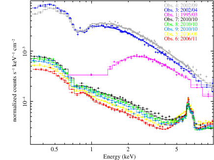
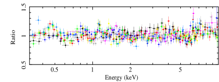
Figure 3: The upper panel shows the data and applied model for all of the spectra listed in Table 2, while the lower panel gives the corresponding residuals for each fit.

3.2 Power Law Normalisation and Neutral Absorber Covering Fraction Correlation

For the large column densities measured by the model defined above, there is an intrinsic degeneracy between the normalisation of the powerlaw continuum and the covering fraction of the neutral absorber. It was necessary therefore to take this effect into account when determining the true errors on these parameters for ASCA Obs. 1 and XMM-Newton Obs. 5 - 9 (where the covering fraction is $>$ 80 per cent in each case). To calculate the true errors on these parameters, the two dimensional confidence levels for these parameters were plotted for the 68, 90, and 99 per cent levels of confidence, which correspond to deviations in the $\chi^{2}$ best-fit value of 2.3, 4.61, and 9.21 respectively (Avni, 1976). The 90 per cent confidence level errors for these parameters can then be measured from the upper and lower bounds of the 90 per cent confidence contours. The errors quoted in Table 2 for these parameters have been measured in this way. The confidence contours for ASCA Obs. 1 and XMM-Newton Obs. 5-9 are shown in Figure 4.

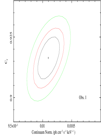
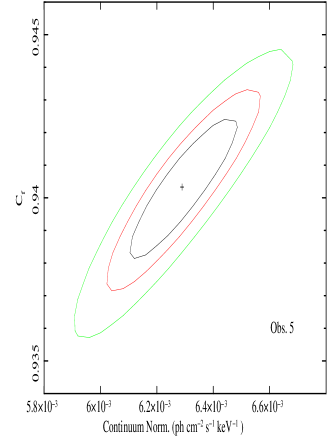
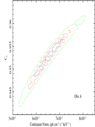
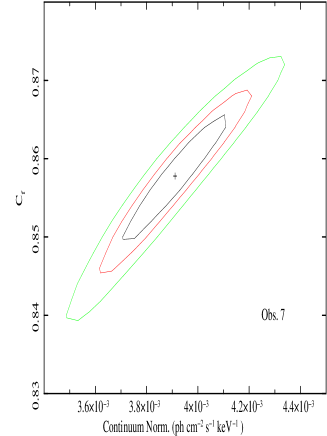
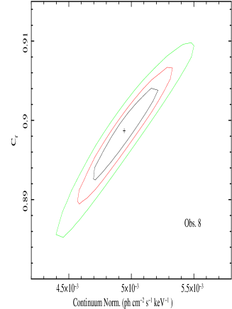
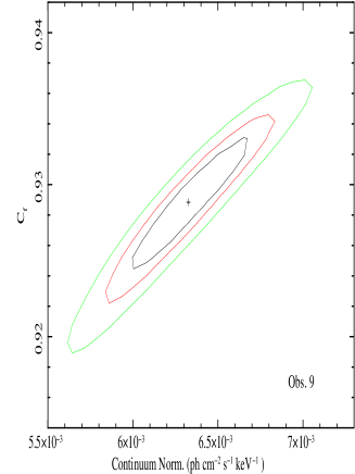
Figure 4: The 68 (black), 90 (red) and 99 (green) per cent confidence contours for power law normalisation and covering fraction of the neutral absorber for ASCA Obs. 1 and XMM-Newton Obs. 5 - 9. The strong correlation between these two parameters is clearly present in Obs. 5 - 9. For Obs. 1 the effect is less pronounced since for these data the neutral absorber component is less prominent due to a lower column density (N${}_{\text{H}}$ $\sim$ 2$\times$10²²).

3.3 Tied Spectral Components

When defining the global model, the ionised absorber components were tied to a common value for each of the spectra, assuming that they do not vary over the time scale of observation. The ionised absorbers have little effect on the low-state spectra, where neutral absorption dominates, and therefore can only be reliably constrained by the high-state spectra. Using spectra 3 and 4, it is therefore possible to set a lower limit on the time scales over which the ionised absorbers remain constant. To do this, the model was again applied to the 2002 XMM-Newton spectra, this time also allowing the column densities and ionisation parameters of the ionised absorbers to vary for both spectra. The best-fit values for the ionised absorber components are given in Table 3. Allowing the ionised absorber components to be variable marginally improves the fit by $\Delta\chi^{2}$ = 29 for 4 DOF. However, from inspection of the parameters and their errors listed in Table 3, it can be seen that the parameters of the second warm absorber component are statistically consistent, while the ionisation parameter of the first warm absorber varies slightly between the two measurements. Therefore it can be concluded that these components are not observed to vary significantly between Obs. 3 and 4.

Table 3: Best-fit parameters for the ionised absorber components when allowed to be free to vary for the 2002 high-state spectra. Column densities, N${}_{\text{H}}$ in units of 10²² cm^-2, ionisation parameters, $\xi$, in units of erg cm s^-1.

Obs. $\#$	Warm Absorber1		Warm Absorber2
	N${}_{\text{H}}$	Log($\xi$)	N${}_{\text{H}}$	Log($\xi$)
3	1.2${}^{+0.3}_{-0.2}$	2.00${}^{+0.16}_{-0.2}$	0.39${}^{+0.10}_{-0.03}$	0.27${}^{+0.08}_{-0.16}$
4	0.9$\pm{0.3}$	1.54${}^{+0.2}_{-0.19}$	0.39${}^{+0.13}_{-0.05}$	0.27${}^{+0.06}_{-0.2}$

The global spectral model also assumes that the spectral index of the power law is invariant between each of the spectra. To investigate if this assumption is valid, the spectral index was allowed to be free to vary for each observation in the global fit. The resultant best fit values were in the range 1.933 - 2.068. This lack of dramatic variability indicates that this component is adequately represented by a model that assumes an invariant spectral index.

The reflection component (pexmon in xspec) was also assumed to remain constant over the time scale of observation. To test this, the model was fit as described in Section 3.1, but also allowing the normalisation of the pexmon component to be free to vary for each observation. For each of the low-state spectra and Obs. 4, the normalisation was found to be consistent with the average value quoted in Table 2. For Obs. 1 and 3, the normalisation was found to be slightly higher than the average value (6 $\pm$ 2$\times$10^-3 ph keV^-1 cm^-2 s^-1), which may be linked to the higher intrinsic flux at these epochs. In order to test for obscuring material on the LOS to the reflection component, a neutral absorption component (zpcfabs) was applied to pexmon. This model was fit with each parameter (except for the column density of the additional absorption component) tied to the best fit values given in Table 2. This fit gave column density values $\leq$ 8$\times$10${}^{\text{20}}$, consistent with the assumption that the pexmon component is not observed through the same absorbing medium that obscures the primary emission.

3.4 Variable Spectral Components

The model defined in section 3.1 proposes that the dramatic spectral variability is due primarily to variations in the neutral absorber obscuring the AGN primary emission. However, an alternate explanation for such dramatic spectral variability is that the emission from the active nucleus has faded, or switched off, leaving only reflected spectral imprints as indications of past activity (Guainazzi et al., 1998; Gilli et al., 2000; Matt, Guainazzi & Maiolino, 2003). To test if this is the case in H0557-385, the global model was again applied to each of the low-state spectra, however this time the neutral absorption component was removed. This results in a very poor fit ($\chi^{2}_{\nu}$ = 5.42), demonstrating that the spectral variations in H0557-385 cannot be accounted for by only considering changes in the primary emission. In addition, it can be seen from Figure 2 that emission at soft X-ray energies has increased in 2010 with respect to 2006, suggesting that nuclear emission is leaking through the absorber. This observation provides further evidence in favour of the partial covering model adopted in this analysis.

It was also assumed in section 3.1 that the intervening gas is composed of neutral material. The validity of this assumption was investigated by testing the effect of a variable absorber composed by ionised material. This test was performed by replacing the neutral absorption component (zpcfabs in xspec) with an ionised absorption component (zxipcf in xspec). This model was fit to the low-state XMM-Newton data, with the following parameters left free to vary for each of the spectra: the column density, covering fraction, and ionisation parameter of the ionised absorber, and the normalisation of the intrinsic power law. Statistically, this model provides a better fit, with $\Delta\chi^{2}$ = 102 for 5 DOF when compared to the model where absorption is produced by neutral gas. However, the inclusion of the ionised absorber yields a much higher value of the power law photon index i.e. $\Gamma$ $\simeq$ 2.6. If the power law is forced to be the same as in the global model with neutral absorption (i.e. by fixing $\Gamma$ $\simeq$ 2), a poorer fit is found ($\Delta\chi^{2}$ = 46 with an increase of 1 DOF).

Figure 5 shows that the change in the power law slope is probably the only observable that can be effectively used to gauge the ionization state of the variable absorber, because the ionised absorber imprints very mild absorption features on the continuum, which are virtually undetectable with CCD data at this flux. Nonetheless, the neutral and ionised absorber models present different spectral indices when fitted to the low-state data, as shown in the figure. This difference is mostly appreciable above 10 keV, a region of the spectrum that is not well sampled by current data. In fact, the data accumulated by the BAT instrument onboard Swift (in the energy range 15 - 150 keV) are integrated over a long time period, (70 months, Baumgartner et al., 2013), therefore an absorber measured in the BAT spectrum might actually be the combined result of mixed spectral states. Therefore, the averaged BAT spectrum is not appropriate for constraining the ionised absorber model at high energies.

It is noted that the measured unabsorbed intrinsic power law spectral index of $\sim$ 2 is more in agreement with the mean value of the spectral index in the 3 - 10 keV range, $<\Gamma_{3-10}>$ = 1.91 $\pm$ 0.07, found by Nandra et al. (1997), by modelling a sample of 18 Seyfert 1 galaxies observed by ASCA and with the value $<\Gamma>$ = 1.89 $\pm$ 0.11 measured by Piconcelli et al. (2005) in the 2 - 12 keV spectra of a sample of 40 QSO from the Palomar-Green (PG) Bright Quasar Survey sample. This remark provides further support to the assumption of a variable absorber composed of neutral material.

Finally, it is also possible that the absorbing medium becomes ionised in response to the increase in intrinsic flux from the source during the high-state epoch. This may lead to a decrease in the opacity of the absorbing medium, with the column density falling with increasing intrinsic flux (e.g. Pounds et al., 2004). However, this effect is not expected to occur in H0557-385, since the analysis carried out in A06 has shown that the 2002 RGS spectra require absorption by neutral material.

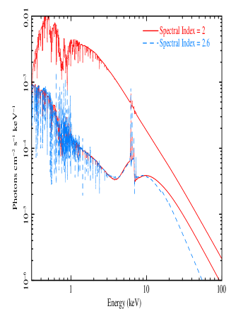
Figure 5: A comparison between the ionised and neutral absorption models is shown. The red lines show the high and low state neutral absorption models with $\Gamma$ $\simeq$ 2. The dashed blue line represents the ionised absorption model which requires $\Gamma$ = 2.6. It is noted here that the intensities of the emission lines around 6 keV are not exactly aligned. This is due to the fact that the neutral absorption models (red lines) were fit using both high- and low-state spectra, while the ionised absorber model was fit using only the low-state spectra, thus giving slightly different values for the normalisation of the pexmon component.

3.5 Results from the Swift Monitoring

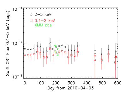
Figure 6: Historic fluxes from the Swift XRT data obtained from 2010 March to 2011 November. For comparison, the figure includes also the three contemporaneous XMM-Newton observations of 2010 October. The three data points are all concentrated at Day 200 and can be recognized thanks to the smaller error bars compared to the Swift ones.

Due to the low count rate, the Swift spectra were rebinned with 5 counts per channel and the Cash statistic was applied for spectral fitting. Although each individual spectrum provides only basic information on the spectral shape of the source, it is very clear that all Swift snapshots caught H0557-385 still in the lowest flux state of 2006 and 2010. Therefore, the flux was simply measured in the 0.4 - 2 keV and 2 - 5 keV bands by fitting a power law to the XRT spectra. From the historic light curve presented in Figure 6, it is evident that during the Swift monitoring, which lasted approximately 1.5 years, the source does not undergo extreme variability (as between the states of 1995, 2002, and 2006). In addition, it is noted that the data obtained by the Swift UVOT show that no significant variability is detected at UV/optical wavelengths for the entire duration of the monitoring. This information will be taken into account in the discussion presented in Section 4.

3.6 Optical Spectroscopy of the BLR and Optical/UV photometry from XMM-Newton Optical Monitor

As the integrated emission line spectrum of H0557-385 is likely affected by internal extinction and the observed continuum includes contribution from the host galaxy, it is first necessary to correct for these two effects before assessing if the AGN varied during the different pointings.

Both internal extinction and contribution of stellar light were determined using the code starlight (Cid Fernandes et al., 2004, 2005; Mateus et al., 2006; Asari et al., 2007). Basically the code fits an observed spectrum O_λ with a combination, in different proportions, of a number of simple stellar populations (SSPs). In addition, in trying to describe the continuum of a Seyfert 1, the contribution of central engine should also be included. Usually this component is represented by a featureless continuum (FC; e.g. Koski (1978)) of powerlaw form that follows the expression F_λ $\propto$ $\lambda^{\alpha}$. Therefore, this component was also added to the base of elements.

Extinction is modelled by starlight as due to foreground dust, and parametrised by the V-band extinction A_v. The extinction law of Cardelli, Geoffrey & Mathis (1989) was used in this procedure as it is widely used in AGNs.

The synthesis carried out with starlight shows that 30$\%$ of the continuum emission at H$\beta$ is due to stellar population. Also, it shows that the observed continuum is affected by an A_v of 1.63, which translates into an internal extinction E(B-V) of 0.53. This latter value is in very good agreement with the E(B-V) of 0.54$\pm$0.08 derived from the line flux ratio H$\alpha$/H$\beta$ measured in the observed spectrum (adopting an intrinsic Balmer decrement of 3.1), giving additional support to the spectral synthesis results. Therefore, after correcting the three spectra for an E(B-V) of 0.53 and subtracting the stellar population, we are left with the continuum that can be attributed entirely to the AGN.

In order to determine if H0557-385 truly varied during the three visits, the method described in Peterson et al. (1991) was followed. It consists of using the strong, narrow [O iii] $\lambda$5007 line as an internal flux standard. The large spatial extend of the NLR and the low electron density (which implies in a very long recombination time) tend to damp out the effect of any short-term variation of the ionising continuum. Therefore, by making the well-justified assumption that the narrow line flux F${}_{\rm[O\,{\textsc{iii}}]}$ is constant over the time scale of interest, variability in the continuum and the broad component of the H$\beta$ line can be discerned by measuring the ratios F_λ/F${}_{\rm[O\,{\textsc{iii}}]}$ and F${}_{\rm H\beta_{BC}}$/F${}_{\rm[O\,{\textsc{iii}}]}$, where F_λ refers to the continuum flux at some specific wavelength (here, taken to be 4870 Å  as in Peterson et al. (1991), in the laboratory rest frame) and F${}_{\rm H\beta_{BC}}$ is the integrated flux in the broad component of the H$\beta$ line. Because the spectra also included H$\gamma$, the ratio F${}_{H\gamma_{BC}}$/F${}_{\rm[O\,{\textsc{iii}}]}$ is also included as a consistency check, where F${}_{H\gamma_{BC}}$ refers to the flux of the broad component of that line. It was decided that the H$\alpha$ line would not be used in this analysis because it is too far in wavelength from [O iii] $\lambda$5007, making it susceptible to atmospheric dispersion effects, considering that the position angle during the observations was not aligned along the parallactic angle.

Because the three spectra were taken using the same telescope and instrument setup, it is perfectly valid to measure the above line ratios for each date and then compare these ratios among the different dates without the need of any normalisation. However, the observations of November 03 and January 30 have also been normalised to the [O iii] flux.

Table 4 lists the line fluxes measured in the three spectra. In order to deblend the broad and narrow components from the observed profile, it was assumed that both H$\beta$ and H$\gamma$ can be represented by a combination of Gaussian profiles. For these two H i lines, two components were always necessary. For each of the three different dates, an excellent agreement was found in the number of components, full-width at half maximum (FWHM) values, and integrated emission line fluxes.

It was found that the narrow component of H$\beta$ has a FWHM of 910 $\pm$ 40 km s^-1 in velocity space. The broad component displayed a FWHM of 3140 $\pm$ 90 km s^-1. These values are already corrected in quadrature by an instrumental broadening of 200 km s^-1, measured from the sky lines present in the spectra.

It is interesting to note that in all three spectra, the peak of the broad component of the Balmer lines is blueshifted relative to that of the narrow component by 11 Å or 680 km s^-1. The position of the narrow component of the H i lines as well as that of [O iii] $\lambda$5007 coincides with the systemic velocity. These results indicate that part of the BLR in H0557-385 may be in an outflow.

Table 4 also lists the line ratios derived from the optical observations. The lack of any variability between the three visits is evident, as the ratios measured in the spectra agree within the uncertainties (3$\sigma$). Therefore, it is concluded that the source remained stable during the sampled period.

Table 4: Optical emission line fluxes measured from the optical spectra of H0557-385.
^a In units of 10^-13 erg cm^-2 s^-1
bContinuum flux at 4870 Å. In units of 10^-13 erg cm^-2 s^-1 Å^-1

	2010-10-17	2010-11-03	2011-01-30
Line Fluxa
[O iii] $\lambda$5007	5.02$\pm$0.23	5.2$\pm$0.19	3.48$\pm$0.15
H$\beta_{NC}$	3.14$\pm$0.20	3.24$\pm$0.16	2.17$\pm$0.12
H$\beta_{BC}$	10.51$\pm$0.71	10.9$\pm$0.53	7.25$\pm$0.41
H$\gamma_{NC}$	1.64$\pm$0.24	1.74$\pm$0.28	1.14$\pm$0.27
H$\gamma_{BC}$	3.14$\pm$0.72	3.98$\pm$0.77	2.79$\pm$0.95
F${}_{4870}^{b}$	0.11$\pm$0.02	0.12$\pm$0.03	0.08$\pm$0.02
Flux Ratio
F4870/F${}_{[O\,{\textsc{iii}}]}\times$4870 Å	107$\pm$20	112$\pm$28	112$\pm$19
FHβ/F${}_{[O\,{\textsc{iii}}]}$	2.1$\pm$0.1	2.1$\pm$0.1	2.1$\pm$0.1
FHγ/F${}_{[O\,{\textsc{iii}}]}$	0.6$\pm$0.2	0.8$\pm$0.2	0.8$\pm$0.3

The ultraviolet flux densities have been checked in the M2 and W1 filters (2310 and 2910 Å) from the OM telescope onboard XMM-Newton, which observed simultaneously to the X-ray instruments. These OM data are available for all XMM-Newton observations but one (2006 November). The OM data do not reveal significant variations in any band, therefore it is concluded that the variability of the X-ray emission observed over the years is not related to variation in the ultraviolet source.

4 Discussion

The multi-epoch spectral model defined in Section 3.1 has shown that H0557-385 is a remarkable example of X-ray absorption variability. The emergent picture is that of an AGN in which most of the spectral features show no variation over the time scale of observation. Instead, the flux variability of this source can be attributed entirely to neutral material attenuating the AGN primary emission. Based on this, a physical discussion of the constant spectral components will first be provided, while an investigation into the nature of the X-ray absorber will be given in Sections 4.2 and 4.3.

4.1 Physical Interpretation of the Constant Spectral Components

The Fe K emission line complex that dominates the low-state spectra is also detected in the intermediate- and high-state spectra, though its shape is less pronounced due to the higher intrinsic flux. This feature has been modelled using a Compton reflection component, where the normalisation has been determined to remain approximately constant for each of the low-state spectra (see Section 3.3). This, along with the fact that the model component (pexmon) is not required to be absorbed by the variable neutral absorption that attenuates the intrinsic power law (also Section 3.3), suggests that this feature originates primarily from material that is exterior to the X-ray absorber. Considering that X-ray variability is often associated with material originating in the BLR region or inner torus, this evidence would then be in favour of an extended torus origin for the reflecting material, as expected by the the Unification model for AGN (Antonucci, 1993). Though this feature has been adequately accounted for by assuming constant reflection of the primary emission, some failure of the model is evident from positive residuals present at $\sim$ 6.4 keV (see Figure 3). It is possible that an additional contribution to the Fe K emission complex may originate from more internal regions of the torus that may partake in continuum absorption (see Section 4.3). This would contaminate the extended (and therefore constant) Fe K emission region with emission from material that may be variable on shorter time scales. However, Fe K$\alpha$ emission from material originating at smaller distances from the continuum source (e.g. the accretion disk) is ruled out from the absence of a broad relativistic component in this feature (L09).

In addition to the power law component, characteristic of AGN emission, the soft X-ray spectra of this source show evidence for absorption by ionised material that is present in two phases (a feature also reported in A06 and L09). It has been shown that the warm absorber components are not observed to vary between Obs. 3 and 4 (see Section 3.3 and Table 3). While the exact origin of the warm absorbers observed in AGN is not well established, a study based on a sample of 23 AGN (Blustin et al. 2005) showed that this component is likely to originate in outflows from the circumnuclear torus (see also Kaastra et al. 2012), or even at kpc scale, as recently proposed by Di Gesu et al. (2013) for the source 1H 0419-577. Such an origin for the warm absorption in this source is tentatively supported by the lack of short term variability in the properties of the warm absorbers, since smaller distances from the SMBH would imply more rapid variability (for recent examples see Longinotti et al. (2013) and Gofford et al. (2014)).

As discussed in Section 3.1, the global model required an emission component (apec) to account for residuals present in the soft X-ray band. Emission in the 0.5 - 2 keV spectrum is expected to occur from gas photoionised by the AGN (Bianchi, Guainazzi & Chiaberge, 2006; Guainazzi & Bianchi, 2007), as well as gas ionised by stellar activity in the host galaxy (LaMassa, Heckman & Ptak, 2012). The low statistical quality of the RGS data makes it difficult to distinguish between these different processes, however, the following simple diagnostics can be used to determine which process is more likely.

First, if it is to be assumed that the luminosity of this component is entirely due to galactic star formation, an upper limit on the star formation rate (SFR) in the host galaxy can be determined via the relation SFR = 2.2$\times$10^-40 L_0.5-2 M_⊙ yr^-1 (Ranalli, Comastri & Setti, 2003). From the apec luminosity, L${}^{\text{APEC}}_{\text{0.5-2}}$ = 1.36 $\pm$ ${0.07}\times$10⁴¹ erg s^-1, the estimate for the SFR is $\simeq$ 29.9 $\pm$ 1.5 M_⊙ yr^-1. This SFR is unusually high and would classify H0557-385 as a starburst galaxy, as these objects typically present SFRs of 5 - 50M_⊙ yr${}^{\text{-1}}$ within a region of 0.1 - 1 kpc extent (Kennicutt, 1998). As the optical spectra do not show any sign of young stellar population compatible with a starburst activity, these results suggest that it may not be appropriate to attribute the emission of the X-ray component entirely to star formation.

Following the method described in Bianchi, Guainazzi & Chiaberge (2006), the ratios of Oiii to soft X-ray flux (using the flux of the APEC component, F${}^{\text{APEC}}_{\text{0.5\,-\,2}}$ = 5.4 $\pm$ 0.3$\times$10${}^{\text{-14}}$ erg cm${}^{\text{-2}}$ s${}^{\text{-1}}$, reported in Section 3.1) for the optical observations 2010-10-17, 2010-11-03, 2011-01-30 were calculated to be 9.3, 9.6, and 6.4 respectively. These ratios are in the same range as those reported in Bianchi, Guainazzi & Chiaberge (2006) for a sample of Seyfert 2 galaxies in which the soft X-ray emission regions have been shown to be concident in spatial extent with the NLR, as mapped by the Oiii emission. This evidence supports the view that the 0.5 - 2 keV emission in this source may originate from the photoionisation of NLR gas, rather than from star formation in the host galaxy.

4.2 Physical Structure of the AGN H0557-385

In attempting to provide a physical interpretation of the spectral features observed in H0557-385, it is instructive to first establish a picture of the AGN structure based on its physical properties. Using Equation 4 from Zamfir et al. (2010), it is possible to derive an estimate for the black hole mass if the FWHM of the broad component of the H$\beta$ line and the luminosity of the continuum at 5100 Å are known. Using the SOAR/Goodman optical spectrograph, the flux of this source at 5100 Å was measured to be 1.02$\pm 0.03\times$10${}^{\text{-14}}$erg s^-1 cm^-2 Å^-1, which corresponds to a luminosity 5100L₅₁₀₀ = 1.31$\pm 0.04\times$10${}^{\text{44}}$erg s^-1. From this result, and the FWHM of the broad component of the H$\beta$ line given in Section 3.6, the mass of the central black hole was found to be M_BH $\sim$ 6.4$\times$10⁷M${\rm\odot}$.

The black hole mass can also be determined from the luminosity and FWHM of the broad component of the H_α line, using Equation 9 from Greene & Ho (2005). The flux of the broad component of the H$\alpha$ line was measured to be F${}_{H\alpha_{BC}}$ = 1.30$\pm 0.05\times$10${}^{\text{-12}}$erg cm^-2 s^-1, giving a luminosity L${}_{H\alpha_{BC}}$ = 3.23$\pm 0.14\times$10${}^{\text{42}}$ erg s^-1. The FWHM was measured to be 4293 km s${}^{\text{-1}}$. From these results, it was found that the value for the black hole mass, M_BH $\sim$ 6.4$\times$10⁷M${\rm\odot}$, agreed with the limits of Equation 9 from Greene & Ho (2005). Therefore, this value will be adopted for the remainder of this analysis.

Hereafter, a linear size of the X-ray source is assumed to be equal to D_s $\simeq$ 10R${}_{\text{g}}$, where R${}_{\text{g}}$ = GM${}_{\text{BH}}$/c², as suggested for other AGN by micro-lensing (Chartas et al., 2002, 2009) and occultation (Risaliti et al., 2007) experiments. It is noted however, that the data presented here do not show the same ingress/egress detail that was available for NGC 1365. Using the value for the black hole mass given above gives D${}_{\text{s}}$ $\simeq$ 1$\times$10¹⁴ cm.

Next, the dust sublimation radius will be estimated. The dust sublimation radius was proposed as an upper boundary on the BLR (Netzer & Laor, 1993), interior to which dust grains are evaporated by emission from the central source. This radius, which is often taken as representative of the inner boundary of the dusty torus, is given by

$$\mathrm{R_{d}\simeq 0.4\left(\frac{L}{10^{45}\,erg\,s^{-1}}\right)^{1/2}\left(\frac{1500\,K}{T_{sub}}\right)^{2.6}pc}$$ (1)

(Nenkova et al., 2008b) where L is the bolometric luminosity, and T${}_{\text{sub}}$ is the dust grain evaporation temperature, generally taken to be the evaporation temperature of graphite grains, T $\sim$ 1500 K (Barvainis, 1987). It is noted here that the sharp boundary given by Equation 1 is an approximation. In reality the transition from dusty to dust-free regions is gradual, the radius at which dust grains can exist being dependent on the grain radii. Taking the maximum luminosity measured by the EPIC best-fit model (Obs. 4, Table 2) and applying a bolometric correction of 20 (Vasudevan & Fabian, 2007)) gives a bolometric luminosity of L_BOL = 2.5$\times$10⁴⁵ erg s^-1. Inserting this value into the above equation gives R${}_{\text{d}}\simeq$ 2$\times$10¹⁸ cm ($\sim$ 0.6 pc). This result can also be used to estimate the outer edge of the torus, which is expected to lie in the range R${}_{\text{out}}$ $\simeq$ 5 - 30 R${}_{\text{d}}$ (see Miniutti et al., 2014, and reference therein). Taking the upper bound of R${}_{\text{out}}$ = 30 R${}_{\text{d}}$ gives R${}_{\text{out}}$ $\simeq$ 5.5$\times$10¹⁹ cm ($\sim$ 18 pc).

It is expected that the broad optical emission lines observed in AGN originate from material that is interior to the dust sublimation radius. From optical spectroscopy (Rodríguez-Ardila, Pastoriza & Donzelli, 2000) three components of the broad H$\alpha$ emission line have been detected in H0557-385 with FWHM that correspond to 1035, 2772, and 11000 km s^-1 in velocity space. Using the correction factor $\frac{\sqrt{3}}{2}$, which is appropriate when considering a spherical BLR (Zhang & Wu, 2002), the orbital velocities of the BLR clouds can be estimated from these line widths. The FWHM of the lines given above correspond to cloud velocities of 900, 2400, and 9550 km s^-1 respectively. Assuming that such clouds are in Keplerian motion around the source gives orbital radii of 1$\times$10¹⁸, 1.5$\times$10¹⁷, and 9$\times$10¹⁵ cm respectively. As expected, these values are all within the upper limit set by the dust sublimation radius.

A second, independent estimate of the distance to the BLR can be made using the relationship between the radius of the BLR and the optical luminosity of the AGN. From Equation 1 in Bentz et al. (2007, see also ()) the radius of the BLR can be found if the luminosity at 5100 Å is known. From the continuum luminosity, 5100L₅₁₀₀ = 1.31$\pm 0.04\times$10${}^{\text{44}}$erg s^-1, the radius of the BLR was found to be R${}_{\text{BLR}}\simeq$ 1$\times$10¹⁷ cm, which is in agreement with the orbital radii of the BLR clouds determined above.

The distance to the BLR can be estimated in a similar way from Equation 1 in Kaspi et al. (2005) using the 2 - 10 keV luminosity. From this relation, and, as before, taking the maximum measured luminosity (Obs. 4, Table 2), the distance to the BLR was found to be R${}_{\text{BLR}}$ $\simeq$ 1$\times$10¹⁷ cm. Again, this value is a good approximation to the previous estimations presented in this section. To allow for ease of comparison, the distance estimates that were derived in this section are illustrated in Figure 7.

Figure 7: An illustration of the AGN geometry as described in Section 4.2. The central black sphere represents the X-ray emission region, with linear size, D${}_{\text{s}}$ = 1$\times$10¹⁴ cm. The spheres labeled a, b, and c represent three components of the BLR at distances of 9$\times$10¹⁵, 1.5$\times$10¹⁷, and 1$\times$10¹⁸ cm respectively. The point labeled x represents the radius of the BLR (1$\times$10¹⁷ cm) as inferred from both the 2 - 10 keV luminosity and the luminosity at 5100 Å (see text for details). Finally, the points R${}_{\text{d}}$ and R${}_{\text{out}}$ represent the estimated inner and outer radii of the circumnuclear torus, at distances of 2$\times$10¹⁸ and 5.5$\times$10¹⁹ cm respectively. The red circles illustrate the possible “clumpy” interior structure of the torus, as discussed in Section 4.3. Distances are not to scale.

4.3 Origin of the X-Ray Absorbers

In the last eight years, H0557-385 exhibited an X-ray spectrum typical of an obscured Seyfert 2 galaxy. The nuclear emission is seen through a partial covering cold absorber with an average column density of $\sim$7$\times$10²³ cm^-2. However, optical spectroscopy simultaneous with some of the X-ray observations in 2010 unveiled a broad-line AGN, consistent with its historical classification as a Seyfert 1. Unless the discrepancy between the optical and the X-ray classification is due to different variability time scales, not adequately monitored by the sparse observations which are available, H0557-385 belongs to the class of AGN that do not fit the 0th order Seyfert Unification scenario. Deep AGN surveys suggest that the fraction of these discrepant object could be as large as 30% (Merloni et al., 2014).

There are two possible explanations for this behaviour: a) the X-ray partial covering clouds are located within the BLR; b) the X-ray absorbing clouds are dust-free (and can be located anywhere). We address in this Section the nature and location of the obscuring clouds in H0057-385, using time constraints derived from our monitoring campaigns.

The first evidence of dramatic X-ray absorption in this source is the transition from the intermediate-state (1995) to the earliest unabsorbed state (2000). The ASCA data (1995) suggest a moderate column density (N${}_{\text{H}}$ $\sim$ 2$\times$10²² cm^-2) neutral absorber covering more than 90 per cent of the X-ray emitting region, while the BeppoSAX data (2000) show the source in an unabsorbed state. Assuming the simplest possible geometry, where a cloud moving with transverse velocity, V${}_{\text{c}}$, with respect to our LOS moves a distance that is equal to at least the linear size of the X-ray source, D${}_{\text{s}}$, in time $\Delta$T, gives the relation D${}_{\text{s}}$ $\leq$ V${}_{\text{c}}\Delta$T.

Rearranging the above equation to find the velocity of the cloud gives V${}_{\text{c}}$ $\geq$ D${}_{\text{s}}$/$\Delta$T, and for $\Delta$T = (T${}_{\text{Obs. 2}}$ - T${}_{\text{Obs. 1}}$) = 1.81$\times$10⁸ s and the value for D${}_{\text{s}}$ derived in Section 4.2, the velocity of the cloud is V_c $\geq$ 5.5 km s^-1. Assuming the cloud is in Keplerian motion around the source, this velocity corresponds to a cloud orbiting at a radius R_c $\leq$ 3$\times$10²² cm from the source. Following the same logic, but considering the obscuring event that occured sometime between Obs. 4 and 5 gives a cloud velocity V${}_{\text{c}}$ $\geq$ 8 km s^-1, refining the orbital radius to R${}_{\text{c}}$ $\leq$ 1$\times$10²² cm. These extreme upper limits on the distance to the cloud arise from the poor time constraints available on these events, and in principle they may be consistent with an absorber located in the dust lane or in the disc of the host Galaxy.

However, the X-ray absorbing clouds are not expected to exist on such large scales, primarily because such an absorber would also obscure the optical BLR, which is clearly observed in this source (see Section 3.6 and Figure 1) during the X-ray obscured states of 2010. An absorber at these scales would also be expected to cause a drop in the UV flux, which again is not observed (Section 3.6). Further evidence of an inner absorber comes from the fact that in 2010 we observe weekly variation of the X-ray obscuration. To investigate the possibility that the absorber is located instead on much smaller scales, the occultation epoch from 2006 to 2011 is examined. It is assumed that the source remains covered by a single absorbing structure from Obs. 5 to the latest Swift observation, giving a minimum occultation time scale of $\Delta$T${}_{\text{occ,1}}^{\text{min}}$ = 1.657$\times$10⁸ s. The linear size of the cloud, D${}_{\text{c}}$, can be related to V${}_{\text{c}}$, $\Delta$T${}_{\text{occ}}^{\text{min}}$, and D${}_{\text{s}}$ according to the relation

$$\mathrm{D_{c}\geq V_{c}\Delta T_{occ}^{min}+D_{s}}$$ (2)

Table 5: The estimated properties of the X-ray absorber obtained by assuming that it either forms part of the BLR or the circumnuclear torus. An absorber column density of N${}_{\text{H}}$ = 7.4$\times$10²³ cm^-2 is assumed (see text for details).

Velocity	$\Delta$T${}_{\text{occ,1}}^{\text{min}}$		$\Delta$T${}_{\text{occ,2}}^{\text{min}}$
(km s-1)	D${}_{\text{c}}$ (cm)	N${}_{\text{e}}$ (cm-3)	D${}_{\text{c}}$ (cm)	N${}_{\text{e}}$ (cm-3)
Broad Line Region
900	$\geq$ 1.5$\times$1016	$\leq$ 5$\times$107	$\geq$ 4.7$\times$1015	$\leq$ 1.6$\times$108
2400	$\geq$ 4$\times$1016	$\leq$ 2$\times$107	$\geq$ 1$\times$1016	$\leq$ 6$\times$107
9550	$\geq$ 1.6$\times$1017	$\leq$ 4.6$\times$106	$\geq$ 5$\times$1016	$\leq$ 1.5$\times$107
Torus
124	$\geq$ 2$\times$1015	$\leq$ 4$\times$108	$\geq$ 7$\times$1014	$\leq$ 1$\times$109
650	$\geq$ 1$\times$1016	$\leq$ 7$\times$107	$\geq$ 3$\times$1015	$\leq$ 2$\times$108

(Miniutti et al., 2014). Inserting BLR cloud orbital velocities (see Section 4.2) into Equation 2 yields the corresponding minimum cloud linear size that would be required to produce the observed obscuration. From these results, an estimate of the electron density, N${}_{\text{e}}$, can be made from the relation N${}_{\text{e}}$ = N${}_{\text{H}}$/D${}_{\text{c}}$, where N${}_{\text{H}}$ can be taken to be the average of the column densities measured in Obs. 5 - 9, giving N${}_{\text{H}}$ = 7.4$\times$10²³ cm^-2. It is noted that during this occultation event, there is no information available on the absorption state of the source between Obs. 6 and 7, which corresponds to a time scale of $\sim$ 4 years, in which time the source may not necessarily remain in an obscured state. Therefore, the values for D${}_{\text{c}}$ and N${}_{\text{e}}$ were also calculated using a minimum occultation time scale that only extends from the start to the end of the Swift monitoring; $\Delta$T${}_{\text{occ,2}}^{\text{min}}$ = 5.07$\times$10⁷ s. As can be seen from Figure 6, the source is not observed to revert to an unobscured state during the course of this monitoring. However, it is noted that even the Swift campaign does not provide a continuous record of the flux of the source; the largest interval between two observations being around three and a half months. Therefore, it is emphasised that all calculations involving $\Delta$T${}_{\text{occ,2}}^{\text{min}}$ are based on the assumption that the source remains in an obscured state for the duration of the monitoring. The cloud properties obtained from these calculations are listed in Table 5.

An alternate interpretation is that the X-ray absorbers form part of the circumnuclear torus. As discussed in Section 4, the inner and outer boundaries of the torus are given by R${}_{\text{d}}$ $\simeq$ 2$\times$10¹⁸ and R${}_{\text{out}}$ $\simeq$ 5.5$\times$10¹⁹ cm respectively. Assuming Keplerian motion, the velocities of material at these distances are V${}_{\text{d}}$ $\simeq$ 650 km s^-1 and V${}_{\text{out}}$ $\simeq$ 124 km s^-1. Following the same formalism as before, the estimated cloud properties were calculated and are listed in Table 5.

The upper limits on the electron density, N${}_{\text{e}}$, of the clouds at the BLR velocity using T${}_{\text{occ,1}}$ are inconsistent with the expected density of the BLR (Popović, 2003), and only marginally consistent if T${}_{\text{occ,2}}$ is employed (see Table 5). On the other hand, the upper limits on the electron density of the clouds at the torus velocity are well consistent with the expected torus density (see Elitzur & Shlosman, 2006; Miniutti et al., 2014). This evidence is considered an indication that the clouds responsible for the X-ray variability episodes in H0557-385 might be dust-free, and located beyond the BLR and within the dust sublimation radius.

As discussed in Section 4.2, the dust sublimation radius does not represent a sharp boundary, but rather a region where gas gradually condenses into dust as distance from the source increases (Nenkova et al., 2008b). From this analysis, it is expected that, while the X-ray absorbing material may be located at the dust sublimation radius, it is likely to be primarily dust free. This is evident from the fact that broad optical emission lines are clearly observed in this source (see Figure 1) during X-ray obscured spectral states. An X-ray absorber located outside the BLR would be expected to obscure the broad emission lines, unless it is dust-free. The fact that broad optical emission lines are observed in this source is strong evidence in favour of a dust-free absorber.

Considering then, that the X-ray absorber must be dust free, it is suggested here that it lies in the intervening region, exterior to the BLR, but interior to the inner boundary of the “dusty” torus. This deduction gives credence to the suggestion that the BLR and torus may in fact be two components of a single, continuous medium that surrounds the nucleus, toroidal in shape, where the dust-to-gas ratio gradually increases in proportion to the distance from the central continuum source, a scenario that has been observationally supported via infrared spectroscopy by the evidence that the outer radius of the BLR is limited by dust (Landt et al., 2014).

Furthermore, in order to fully account for the X-ray spectral variability observed in this source, it must be assumed that the X-ray absorbing medium is not homogeneous, but rather consists of discrete “clumps” (or clouds) of gas, as illustrated in Figure 7. This would explain the observed variation among the low-state spectra, and the subsequent variations in the covering fraction of the absorber, as measured by the spectral model defined in Section 3.1. A clumpy torus absorber would allow intrinsic emission from the AGN to leak through, and give rise to variations in the soft X-ray spectrum, even among obscured states. This phenomenon is clearly observed in H0557-385. Finally, a clumpy absorber would imply that the probability of directly observing the (unobscured) AGN continuum would be finite, and dependent on the individual cloud size and number density. In light of this interpretation, the high-state (unobscured) spectra (XMM-Newton 2002, BeppoSAX 2000) would represent epochs when the observers LOS did not intercept material in the clumpy environment which caused the obscuration event(s) of 2006/2010.

5 Conclusions

In this analysis, the X-ray spectral variability associated with the Seyfert 1 AGN H0557-385 has been interpreted as being due to the occultation of the central emission region by high column density (N${}_{\text{H}}$ $\sim$ 7$\times$10²³ cm^-2) neutral material, covering $\geq$ 80 per cent of the X-ray emission region.

From consideration of the absorption time scales, it has been inferred that the absorbing material forms part of the clumpy circumnuclear torus, at a distance of $\sim$ 2$\times$10¹⁸ cm from the X-ray emission region. The detection of broad optical emission lines in this source implies that the obscuration occurs in a dust-free region within, or very close to, the dust sublimation radius. It may be possible that the LOS grazes the diffuse upper atmosphere of the clumpy torus, which would explain why a Compton-thick absorption state, normally associated with obscuration by the circumnuclear torus, is never observed in this source.

In order to further understand the nature of the absorbing medium in this source, it would be necessary to first observe an “unveiling” event, that is, to monitor the emersion of the central continuum source from the absorbed state. If such observations were available, it may be possible to explore the evolution of the cloud covering fraction with time, and hence place tighter constraints on the geometry and location of the obscuring clouds. In addition, observations of this source at energies $>$ 10 keV would be useful in attempting to determine the ionisation state of the absorbing medium (see Section 3.4). This data would then provide an additional estimate of the distance to the absorbing cloud based on the measured value of the ionisation parameter. This measurement could be possible with deep NuSTAR or Astro-H observations.

References

- Antonucci (1993) Antonucci R., 1993, ARA&A, 31, 473
- Arnaud (1996) Arnaud K. A., 1996, ASP Conf. Ser., 101, 17
- Asari et al. (2007) Asari N. V., Cid Fernandes R., Stasinska G., Torres-Papaqui J. P., Mateus A., Sodré L., Schoenell W., Gomes J. M., 2007, MNRAS, 381, 263
- Ashton et al. (2006) Ashton C. E., Page M. J., Branduardi-Raymont G., Blustin A. J., 2006, MNRAS, 366, 521
- Avni (1976) Avni Y., 1976, ApJ, 210, 642
- Barvainis (1987) Barvainis R., 1987, ApJ, 320, 537
- Baumgartner et al. (2013) Baumgartner W. H., Tueller J., Markwardt C. B., Skinner G. K., Barthelmy S., Mushotzky R. F., Evans P. A., Gehrels N., 2013
- Bentz et al. (2007) Bentz M. C., Denney K. D., Peterson B. M., Pogge R. W., 2007, in Ho L. C., Wang J.-W., eds, The Central Engine of Active Galactic Nuclei. Astron. Soc. Pac., San Francisco, p. 380
- Bentz et al. (2006) Bentz M. C., Peterson B. M., Pogge R. W., Vestergaard M., Onken C. A., 2006, ApJ, 644, 133
- Bianchi, Guainazzi & Chiaberge (2006) Bianchi S., Guainazzi M., Chiaberge M., 2006, A&A, 448, 499
- Bianchi et al. (2009) Bianchi S., Piconcelli E., Chiaberge M., Bailón E. J., Matt G., Fiore F., 2009, ApJ, 695, 781
- Burrows et al. (2005) Burrows D. H. et al., 2005, Space Sci. Rev., 120, 165
- Cardelli, Geoffrey & Mathis (1989) Cardelli J. A., Geoffrey G. C., Mathis J. S., 1989, ApJ, 345, 245
- Chartas et al. (2002) Chartas G., Agol E., Eracleous M., Garmire G., Bautz M. W., Morgan N. D., 2002, ApJ, 568, 509
- Chartas et al. (2009) Chartas G., Kochanek C. S., Dai X., Poindexter S., Garmire G., 2009, ApJ, 693, 174
- Cid Fernandes et al. (2004) Cid Fernandes R., Gu Q., Melnick J., Terlevich E., Terlevich R., Knuth D., Rodigues Lacerda R., Joguet B., 2004, MNRAS, 355, 273
- Cid Fernandes et al. (2005) Cid Fernandes R., Mateus A., Sodré L., Stasinska G., Gomes J. M., 2005, MNRAS, 358, 363
- Dadina (2007) Dadina M., 2007, A&A, 461, 1209
- Di Gesu et al. (2013) Di Gesu L. et al., 2013, A&A, 556, A94
- Dickey & Lockman (1990) Dickey J. M., Lockman F. J., 1990, ARA&A, 28, 215
- Elitzur (2008) Elitzur M., 2008, New Astron. Rev., 52, 274
- Elitzur (2012) Elitzur M., 2012, ApJL, 747, L33
- Elitzur & Shlosman (2006) Elitzur M., Shlosman I., 2006, ApJ, 648, L101
- Fairall, McHardy & Pye (1982) Fairall A. P., McHardy I. M., Pye J. P., 1982, MNRAS, 198, 13P
- Ghisellini, Haardt & Matt (1994) Ghisellini G., Haardt F., Matt G., 1994, MNRAS, 267, 743
- Gilli et al. (2000) Gilli R., Maiolino R., Marconi A., Risaliti G., Dadina M., Weaver K. A., Colbert E. J. M., 2000, A&A, 355, 485
- Gofford et al. (2014) Gofford J. et al., 2014, ApJ, 784
- Greene & Ho (2005) Greene J. E., Ho L. C., 2005, ApJ, 630, 122
- Guainazzi & Bianchi (2007) Guainazzi M., Bianchi S., 2007, MNRAS, 374, 1290
- Guainazzi et al. (1998) Guainazzi M. et al., 1998, MNRAS, 301, L1
- Jaffe et al. (2004) Jaffe W. et al., 2004, Nature, 429, 47
- Jansen et al. (2001) Jansen F. et al., 2001, A&A, 365, L1
- Kaspi et al. (2005) Kaspi S., Maoz D., Netzer H., Peterson B. M., Vestgaard M., Jannuzi B. T., 2005, ApJ, 629, 61
- Kennicutt (1998) Kennicutt R., 1998, ApJ, 498, 541
- Koski (1978) Koski A. T., 1978, ApJ, 223, 56
- Krolik & Begelman (1988) Krolik J. H., Begelman M. C., 1988, ApJ, 329, 702
- LaMassa, Heckman & Ptak (2012) LaMassa S. M., Heckman T. M., Ptak A., 2012, ApJ, 758
- Landt et al. (2014) Landt H., Ward M. J., Elvis M., Karovska M., 2014, MNRAS, 439, 1051
- Longinotti et al. (2009) Longinotti A. L., Bianchi S., Ballo L., de La Calle I., Guainazzi M., 2009, MNRAS, 394, L1
- Longinotti et al. (2013) Longinotti A. L. et al., 2013, ApJ, 766
- Mateus et al. (2006) Mateus A., Sodré L., Cid Fernandes R., Stasinska G., Schoenell W., Gomes J. M., 2006, MNRAS, 370, 721
- Matt, Guainazzi & Maiolino (2003) Matt G., Guainazzi M., Maiolino R., 2003, MNRAS, 342, 422
- Merloni et al. (2014) Merloni A. et al., 2014, MNRAS, 437, 3550
- Miller et al. (2007) Miller L., Turner T. J., Reeves J. N., George I. M., Kraemer S. B., Wingert B., 2007, A&A, 463, 131
- Miniutti et al. (2014) Miniutti G. et al., 2014, MNRAS, 437, 1776
- Nandra et al. (1997) Nandra K., George I. M., Mushotzky R. F., Turner T. J., Yaqoob T., 1997, ApJ, 477, 602
- Nandra et al. (2007) Nandra K., O’Neill P. M., George I. M., Reeves J. N., 2007, MNRAS, 382, 194
- Nenkova et al. (2008a) Nenkova M., Sirocky M. M., Nikutta R., Ž Ivezić, Elitzur M., 2008a, ApJ, 685, 147
- Nenkova et al. (2008b) Nenkova M., Sirocky M. M., Nikutta R., Ž Ivezić, Elitzur M., 2008b, ApJ, 685, 160
- Netzer & Laor (1993) Netzer H., Laor A., 1993, ApJ, 404, L51
- Peterson et al. (1991) Peterson B. M. et al., 1991, ApJ, 368, 119
- Piconcelli et al. (2007) Piconcelli E., Bianchi S., Guainazzi M., Fiore F., Chiaberge M., 2007, A&A, 466, 855
- Piconcelli et al. (2005) Piconcelli E., Jimenez-Bailón E., Guainazzi M., Schartel N., Rodríguez-Pascual P. M., Santos-Lleó M., 2005, A&A, 432, 15
- Popović (2003) Popović L. C., 2003, ApJ, 599, 140
- Pounds et al. (2004) Pounds K. A., Reeves J. N., Page K. L., O’Brien P. T., 2004, ApJ, 616, 696
- Quadrelli et al. (2003) Quadrelli A., Malizia A., Bassani L., Malaguti G., 2003, A&A, 411, 77
- Ranalli, Comastri & Setti (2003) Ranalli P., Comastri A., Setti G., 2003, A&A, 399, 39
- Risaliti et al. (2007) Risaliti G., Elvis M., Fabbiano G., Baldi A., Zezas A., Salvati M., 2007, ApJ, 659, L111
- Rivers, Markowitz & Rothschild (2011) Rivers E., Markowitz A., Rothschild R., 2011, ApJ, 742, L29
- Rodríguez-Ardila, Pastoriza & Donzelli (2000) Rodríguez-Ardila A., Pastoriza M. G., Donzelli C. J., 2000, ApJS, 126
- Sanfrutos et al. (2013) Sanfrutos M., Miniutti G., Agís-González B., Fabian A. C., Miller J. M., Panessa F., Zoghbi A., 2013, MNRAS, 436, 1588
- Schlafly & Finkbeiner (2011) Schlafly E. F., Finkbeiner D. P., 2011, ApJ, 737, 103
- Tristram et al. (2007) Tristram K. R. W. et al., 2007, A&A, 474, 837
- Turner, Netzer & George (1996) Turner T. J., Netzer H., George I. M., 1996, ApJ, 463, 134
- Urry & Padovani (1995) Urry M. C., Padovani P., 1995, PASP, 107, 803
- Vasudevan & Fabian (2007) Vasudevan R. V., Fabian A. C., 2007, MNRAS, 381, 1235
- Wilms, Allen & McCray (2000) Wilms J., Allen A., McCray R., 2000, ApJ, 542, 914
- Zamfir et al. (2010) Zamfir S., Sulentic J. W., Marziani P., Dultzin D., 2010, MNRAS, 403, 1759
- Zhang & Wu (2002) Zhang T. Z., Wu X. B., 2002, ChJAA, 2, 487