Model Hamiltonian for topological Kondo insulator SmB₆

Abstract

Starting from the k$\cdot$p method in combination with first-principles calculations, we systematically derive the effective Hamiltonians that capture the low energy band structures of recently discovered topological Kondo insulator SmB₆. Using these effective Hamiltonians we can obtain both the energy dispersion and the spin texture of the topological surface states, which can be detected by further experiments.

I Introduction

Searching for new topological insulators (TI) has become an active research field in condensed matter physicsQi and Zhang (2011); Hasan and Kane (2010). A topological insulator has insulating and topologically non-trivial bulk band structure giving rise to robust Dirac like surface states, which are protected by time reversal symmetry and have the spin-momentum locking feature. Such topological surface states have several remarkable properties. For example, the suppression of back scattering and localization on the TI surfaceRoushan et al. (2009); Alpichshev et al. (2010); Zhang et al. (2009); Xia et al. (2009); Beidenkopf et al. (2011). Furthermore, if superconductivity is induced on the surface of TIs via proximity effects, the Majorana bound states can be induced Fu and Kane (2008); Santos et al. (2010); Qi et al. (2010). These novel properties make topological insulator a promising platform for the design of spintronics devices and future quantum computing applicationsMoore (2010).

Recently the mixed valence compound SmB₆ has been proposed to be topological insulator and attracts lots of research interestsDzero et al. (2009, 2012); Alexandrov et al. (2013a); Ye et al. (2013); Dzero and Galitski (2013); Lu et al. (2013). Unlike the other well studied topological insulator materials, i.e. the Bi₂Se₃ family, the strong correlation effects in mixed valence TIs are crucial to understand the electronic structure due to the partially filled 4f bandsLu et al. (2013); Weng et al. (2014); Deng et al. (2013). There are two main effects induced by the on-site Coulomb interaction among the f-electrons, one is the strong modification of the 4f band width, the other is the correction to the effective spin-orbital coupling and crystal fieldAlexandrov et al. (2013b); Legner et al. (2014); Werner and Assaad (2013). As a consequence, the band inversion in the modified band structure happens between the 5d and 4f band (with total angular momentum j=5/2) around the three X points in the Brillouin Zone. Unlike the situation in Bi₂Se₃ family, where the band inversion happens between two bands both with the p character and similar band width, the band inversion in SmB₆ happens between two bands with the band widths differing by orders, which leads to very unique low energy electronic structure. Since the band inversion happens at the Zone boundary (X points), which project to three different points in surface Brillouin Zone leading to three different Dirac points on generic surfaces.

Experimentally, the first evidence of topological surface states has been found by transport measurements, and then by angle resolved photo emission spectroscopy (ARPES), Scanning Tunneling Spectroscopy (STS), quantum oscillation magneto-resistance measurementsFrantzeskakis et al. (2013a); Wolgast et al. (2013); Xu et al. (2013); Li et al. (2013); Neupane et al. (2013); Kim et al. (2013); Jiang et al. (2013); Thomas et al. (2013); Yee et al. (2013); Denlinger et al. (2013a); Frantzeskakis et al. (2013b); Ruan et al. (2014); Denlinger et al. (2013b). Unlike the electronic structures in large energy scale, which is mainly determined by the local atomic physics, the topological nature of the electronic structure can be fully described by the quasi-particle structure only, whose form can be determined from the symmetry principles. In the present paper, we will construct a k$\cdot$p model capturing the full topological and symmetry features of the low energy quasi-particle structure, which leads to topological surface states with the renormalized Fermi velocities. All the symmetry allowed terms in the above k$\cdot$p model have been obtained by fitting with the band structure obtained by the LDA+Gutzwiller calculation introduced in a previous paperLu et al. (2013). Such a analytical model gives a clear theoretical description for the quasi-particle structure of SmB₆, which can be widely used in the further studies.

The organization of the present paper is as follows. In Sec.II, we present the crystal structure and band structure of SmB₆. Then we construct the effective models to describe the bulk band structure for this material from the symmetry considerations in Sec.III. Furthermore we calculate surface states and the spin texture on the the (001) surface based on our model Hamiltonian and show that it is consistent with the tight-binding calculation results. Conclusions are given in the end of this paper.

II Crystal structure and band structure

In this section we first describe the crystal structure of the SmB₆ and then discuss the nontrivial topological bulk band structure of it.

crystal structure: SmB₆ has the CsCl-type crystal structure with $Pm\bar{3}m$ space group. The Sm ions are located at the corner and B₆ octahedron are located at the body center of the cubic lattice as shown in Figure 1(a). The corresponding bulk and projected Brillouin zone (BZ) of (001) surface for SmB₆ are shown in Fig.1(b).

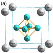
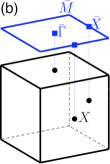
Figure 1: (Color online) (a) The CsCl-type structure of SmB₆with $Pm\bar{3}m$ space group. Sm ions and B₆ octahedron are located at the corner and center of the cubic lattice respectively. (b) The bulk Brillouin zone of SmB₆ (black cubic) and its projection onto the (001) (blue square). The $X$ points (black dots) in the bulk BZ are projected to $\bar{\Gamma}$ and $\bar{X}$ points (blue square points ) in the (001) surface BZ.

electronic structure: Previous electronic structure studies find that in SmB₆ the band inversion happens between Sm 4f bands with total angular momentum $j=5/2$ and one of the 5d bands, which leads to fractional occupation in 4f $j=5/2$ orbitals or "non-integer chemical valence" Beaurepaire et al. (1990); Cohen et al. (1970); Eibschutz et al. (1972); Chazalviel et al. (1976). Since the band inversion happens at three X points in the BZ, where the 4f and 5d states have opposite parities, the Z₂ topological non-trivial band structure is formedKane and Mele (2005); Fu and Kane (2006). In order to include the strong Coulomb interaction among the f electrons, we implement the local density approximation in density functional theory with the Gutzwiller variational method (LDA+Gutzwiller) and apply it to calculate the renormalized band structure of SmB₆.

Here we briefly introduce the LDA+Gutzwiller method, for detailed descriptions please refer to Ref.[Deng et al., 2009; Lu et al., 2013]. The LDA+Gutzwiller method combines the LDA with Gutzwiller variational method, which takes care of the strong atomic feature of the f-orbitals in the ground state wave function. In this method, we implement the single particle Hamiltonian obtained by LDA with on site interaction terms describing the atomic multiplet features, which can be written as,

$$H=H_{LDA}+H_{int}+H_{DC}$$ (1)

where $H_{LDA}$, $H_{int}$ and $H_{DC}$ represent the LDA Hamiltonian, on-site interaction and the double counting terms respectivelyKotliar et al. (2006). The LDA Hamiltonian can be expressed in a tight binding form by constructing the projected Wannier functions for both 5d and 4f bandsKuneÅ¡ et al. (2010); Solovyev et al. (2007); Mostofi et al. (2008).The on-site interactions can be described in terms of Slater integrals as introduced in detail in the previous paperLu et al. (2013). The double counting term $H_{DC}$ subtracts the correlation energy already included in LDA calculation. Within the Gutzwiller approximation, an effective Hamiltonian $H_{eff}$ describing the quasi-particle band structure can be obtained, which describes the low energy dynamics including the topological surface statesLu et al. (2013). To further study the low energy physics of SmB₆, i.e. the behavior of the surface states, a simple k$\cdot$p model Hamiltonian will be very useful. In the next section, we will construct such a model by expanding the $H_{eff}$ near the three X points.

III Model Hamiltonian for SmB₆

In this section, we will systematically derive the effective Hamiltonian near $X$ points based on k$\cdot$p theory combined with the results of first-principle calculations. We only give the effective Hamiltonian at $X_{1}=(0,0,\frac{1}{2})$ point. The effective Hamiltonian at the other two $X$ points can be obtained by acting $C_{4x}$ or $C_{4y}$ rotation operations on the Hamiltonian at $X_{1}$. Using the symmetry group at the $X$ point we can construct the effective k$\cdot$p model near this point and all the parameters used in such a model can be obtained by fitting to the renormalized band structure obtained by LDA+Gutzwiller.

The k$\cdot$p Hamiltonian is obtained from our one-partial effective Hamiltonian

$$H_{eff}\psi_{n,\mathbf{k}}(\mathbf{r})=E_{n,\mathbf{k}}\psi_{n,\mathbf{k}}(\mathbf{r}),$$ (2)

where $\psi_{n,\mathbf{k}}=e^{i\mathbf{k}\cdot\mathbf{r}}u_{n,\mathbf{k}}(\mathbf{r})$ are the Bloch wave functions and the effective Hamiltonian only consists of the kinetic-energy operator, a local periodic crystal potential, and the spin-orbit interaction term:

$$H_{eff}=\frac{p^{2}}{2m}+V(\mathbf{r})+\frac{\hbar}{4m_{0}^{2}c^{2}}(\mathbf{\sigma}\times\nabla V)\cdot\mathbf{p}.$$ (3)

In terms of the cellular functions $u_{n,\mathbf{k}}(\mathbf{r}),$ Eq.(2) becomes

$$H_{\mathbf{k}}u_{n,\mathbf{k}}(\mathbf{r}) \equiv \bigg{[}\frac{p^{2}}{2m}+V(\mathbf{r})+\frac{\hbar}{4m_{0}^{2}c^{2}}(\sigma\times\nabla V)\cdot(\mathbf{p}+\hbar\mathbf{k})$$ (4)

$$+ \frac{\hbar}{m}\mathbf{k}\cdot\mathbf{p}\bigg{]}u_{n,\mathbf{k}}(\mathbf{r})=\epsilon_{n,\mathbf{k}}u_{n,\mathbf{k}}(\mathbf{r}),$$

where $\epsilon_{n,\mathbf{k}}\equiv E_{n,\mathbf{k}}-\frac{\hbar^{2}k^{2}}{2m}$. Expanding the above Hamiltonian at given high symmetry point $k_{0}$, the eigen-equation at $k_{0}+k$ can be obtained by

$$\bigg{[}H_{\mathbf{k}_{0}}+\frac{\hbar}{m}\mathbf{k}\cdot\mathbf{p}\bigg{]}u_{n,\mathbf{k}_{0}+\mathbf{k}}(\mathbf{r})=\epsilon_{n,\mathbf{k}_{0}+\mathbf{k}}u_{n,\mathbf{k}_{0}+\mathbf{k}}(\mathbf{r}),$$ (5)

where we have ignored the k-dependent spin-orbit term, which is usually much small. Once $E_{n,\mathbf{k}_{0}}$ and $u_{n,\mathbf{k}_{0}}$are known, the function $u_{n,\mathbf{k}_{0}+\mathbf{k}}(\mathbf{r})$ can be obtained by treating the term $H_{kp}=\frac{\hbar}{m}\mathbf{k}\cdot\mathbf{p}$ in Eq.(5) as a perturbation. It is more convenient to rewrite the perturbation as

$$H_{kp}=\frac{\hbar}{m}\mathbf{k}\cdot\mathbf{p}=\frac{\hbar}{2m}(k_{+}p_{-}+k_{-}p_{+})+\frac{\hbar}{m}k_{z}p_{z},$$ (6)

where the operator $p_{\pm}=p_{x}\pm ip_{y}$ and $k_{\pm}=k_{x}\pm ik_{y}$.

In the SmB₆ system, we expand the $H_{eff}$ near the three X points. We chose the k$\cdot$p basis function at X point as

$$\left|\frac{3}{2},\frac{3}{2}\right\rangle_{d},\left|\frac{3}{2},-\frac{3}{2}\right\rangle_{d},\left|\frac{5}{2},\frac{5}{2}\right\rangle_{f},\left|\frac{5}{2},-\frac{5}{2}\right\rangle_{f}$$

$$\left|\frac{5}{2},\frac{3}{2}\right\rangle_{f},\left|\frac{5}{2},-\frac{3}{2}\right\rangle_{f},\left|\frac{5}{2},\frac{1}{2}\right\rangle_{f},\left|\frac{5}{2},-\frac{1}{2}\right\rangle_{f},$$ (7)

which can well describe the orbital characters for the eigenstates near the Fermi energy. We can then project the k$\cdot$p Hamiltonian into above basis and the matrix elements of $H_{kp}$ are constrained by the crystal symmetries at $X$ point. The little group at $X$ point is $D_{4h}$, which contains the following symmetry operations:

(1) fourfold rotation along the $z$ direction $\hat{C}_{4z}$ =$e^{-i\frac{2\pi}{4}\hat{J}_{z}}$, where $\hat{J}_{\alpha}$ ($\alpha=x,y,z$) is the operator for the $\alpha$ component of the total angular momentum.

(2) inversion symmetry $\hat{P}=I_{2}\oplus-I_{6}$, where $I_{m}$ is the m$\times$m identity matrix.

(3) time reversal symmetry $\hat{T}$=$\Theta K=e^{-i\pi\hat{J}_{y}}K$, where $K$ is the complex conjugate operator.

(4) twofold rotation along $y$ direction $\hat{C}_{2y}=e^{-i\pi\hat{J}_{y}}$ .

The symmetry operation can help us to reduce the independent parameters that appear in the $k\cdot p$ Hamiltonian. For example, considering the rotation $C_{4z}$ around the $z$ direction, we have

$${}_{d}\left\langle\frac{3}{2},\frac{3}{2}\right|p_{-}\left|\frac{5}{2},\frac{5}{2}\right\rangle_{f}={}_{d}\left\langle\frac{3}{2},\frac{3}{2}\right|C_{4z}^{\dagger}C_{4z}p_{-}C_{4z}^{\dagger}C_{4z}\left|\frac{5}{2},\frac{5}{2}\right\rangle_{f}.$$ (8)

Since ${}_{d}\langle\frac{3}{2},\frac{3}{2}|C_{4z}^{\dagger}={}_{d}\langle\frac{3}{2},\frac{3}{2}|e^{i\frac{2\pi}{4}\frac{3}{2}}$, $C_{4z}p_{\pm}C_{4z}^{\dagger}=e^{\mp i\frac{2\pi}{4}}p_{\pm}$, and $C_{4z}|\frac{5}{2},\frac{5}{2}\rangle_{f}=e^{-i\frac{2\pi}{4}\frac{5}{2}}|\frac{5}{2},\frac{5}{2}\rangle_{f}$, we get that $c_{1}\equiv\frac{\hbar}{2m}{}_{d}\langle\frac{3}{2},\frac{3}{2}|p_{-}|\frac{5}{2},\frac{5}{2}\rangle_{f}$ is invariant under $C_{4z}$ rotation and can be non-zero. While ${}_{d}\langle\frac{3}{2},\frac{3}{2}|p_{+}|\frac{5}{2},\frac{5}{2}\rangle_{f}$ get a minus sign under $C_{4z}$ rotation, which means it must vanish. Following the same procedge, we can get $c_{1}^{\prime}\equiv\frac{\hbar}{2m}{}_{d}\langle\frac{3}{2},-\frac{3}{2}|p_{+}|\frac{5}{2},-\frac{5}{2}\rangle_{f}$ is finite. When considering the 2-fold rotation along the $y$ direction $C_{2y}$, we get the relation between $c_{1}$ and $c_{1}^{\prime}$ as

$$c_{1} = \frac{\hbar}{2m}{}_{d}\langle\frac{3}{2},\frac{3}{2}|p_{-}|\frac{5}{2},\frac{5}{2}\rangle_{f}$$ (9)

$$= \frac{\hbar}{2m}{}_{d}\langle\frac{3}{2},\frac{3}{2}|C_{2y}^{\dagger}C_{2y}p_{-}C_{2y}^{\dagger}C_{2y}|\frac{5}{2},\frac{5}{2}\rangle_{f}$$

$$= -\frac{\hbar}{2m}{}_{d}\langle\frac{3}{2},-\frac{3}{2}|p_{+}|\frac{5}{2},-\frac{5}{2}\rangle_{f}=-c_{1}^{\prime}.$$

Due to the time-reversal symmetry, the $c_{1}$ can be chosen to be real. Similar considerations can be used to calculate all matrix elements and we obtain the effective Hamiltonian, which is invariant under all symmetry operations at $X$ point up to the first order of $k$,

$$H_{X}=\left(\begin{array}[]{cccccccc}\epsilon_{d}&0&c_{1}k_{+}&c_{2}k_{z}&c_{3}k_{z}&c_{4}k_{+}&c_{5}k_{-}&0\\ &\epsilon_{d}&c_{2}k_{z}&-c_{1}k_{-}&-c_{4}k_{-}&c_{3}k_{z}&0&-c_{5}k_{+}\\ &&\epsilon_{f_{5}}&0&0&d_{1}&0&0\\ &&&\epsilon_{f_{5}}&d_{1}&0&0&0\\ &&&&\epsilon_{f_{3}}&0&0&0\\ &&\dagger&&&\epsilon_{f_{3}}&0&0\\ &&&&&&\epsilon_{f_{1}}&0\\ &&&&&&&\epsilon_{f_{1}}\end{array}\right),$$ (10)

where $\epsilon_{d}=D+D_{xy}(k_{x}^{2}+k_{y}^{2})+D_{z}k_{z}^{2}$, $\epsilon_{f_{i}}=F_{i}+F_{i,xy}(k_{x}^{2}+k_{y}^{2})+F_{i,z}k_{z}^{2}$ ($i=5,3,1$) and $k_{\pm}=k_{x}\pm ik_{y}$. The parameters are listed in Table.1. The fitted energy dispersion for SmB₆ is plotted in Fig.2. It shows that our model Hamiltonian with eight bands captures the main features of the band dispersion near $X$ point.

Table 1: Parameters in our model Hamiltonian fitted for SmB₆, where the unit of energy is eV and the unit of length is the lattice constant.

$D$	$D_{xy}$	$D_{z}$	$F_{1}$	$F_{1,xy}$	$F_{1,z}$
-1.5698	29.9233	18.2502	-0.0532	-0.0020	-0.0300
$F_{3}$	$F_{3,xy}$	$F_{3,z}$	$F_{5}$	$F_{5,xy}$	$F_{5,z}$
0.0163	-0.5776	-0.4476	-0.0164	-0.1543	-0.1543
$c_{1}$	$c_{2}$	$c_{3}$	$c_{4}$	$c_{5}$	$d_{1}$
-0.2787	-0.318	-0.502	-0.5960	0.0021	-0.0132

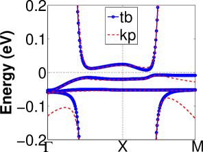
Figure 2: The energy dispersion obtained from our model Hamiltonian with 8 bands (thin red line) is compared with that from tight-binding calculations (thick blue line). Here $M$ to $X$ lines represents the dispersion along the $k_{x}$ direction while the $X$ to $\Gamma$ lines is for the $k_{z}$ direction..

An important physical consequence of the non-trivial topological band structure is the existence of Dirac like surface states with chiral spin texture. The $X$ points in the bulk BZ are projected to $\bar{\Gamma}$ and $\bar{X}$ points in the (001) surface BZ as shown in Fig.1(b). To study the surface state and the spin texture near $\bar{\Gamma}$ point, we consider a thick slab limited in $z\in[-d/2,d/2]$ with open boundary conditions, where $d$ is the thickness of the slab in $z$ direction. Now $k_{z}$ is not a good quantum number which should be replaced by $-i\partial_{z}$. The eigenwave function will be given by $\psi(k_{x},k_{y},z)$, which can be expanded using basis {$\varphi_{n}(z)=\sqrt{2/d}\;sin[n\pi(z+\frac{d}{2})/d]$} $(n=0,1,2,3,...)$. The Hamiltonian for the slab structure is written as $H_{\bar{\Gamma},mn}^{slab}(k_{x},k_{y})=\langle\varphi_{m}(z)|H_{s}(k_{x},k_{y},-i\partial_{z})|\varphi_{n}(z)\rangle$. The surface states near $\bar{\Gamma}$ point can be calculated directly from $H_{\bar{\Gamma}}^{slab}(k_{x},k_{y})$. For the surface states and spin texture near $\bar{X}$ point, we can use the same method but change the $z$ direction to $x$ direction. The calculated surface states near $\bar{\Gamma}$ and $\bar{X}$ points are shown in Fig.3(b) and compared with the results from tight-binding calculation Fig.3(a). There are three Dirac cone like surface states. One located at $\bar{\Gamma}$ points, the other two located at two $\bar{X}$ points, which is different with most of the known 3D topological insulators, such as B$i_{2}$Se₃.

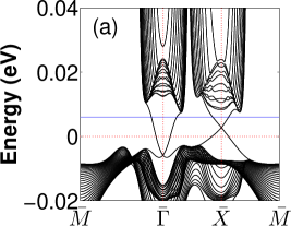
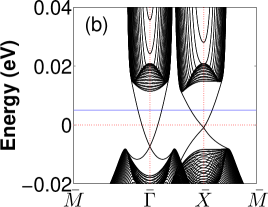
Figure 3: The (001) direction surface states near $\bar{\Gamma}$ and $\bar{X}$ point, (a) from the tight-binding model; (b) from the k$\cdot$p model results. The blue solid line indicates the energy for the spin-texture calculations.

From $H_{\bar{\Gamma},\bar{X}}^{slab}$ we can further get the spin texture of the surface states near $\bar{\Gamma}$ and $\bar{X}$ points. The spin texture at the energy of 6meV is shown in Fig.4, which shows a strong spin-moment locking on the surface states. We will discuss the spin texture from the symmetry consideration below.

  

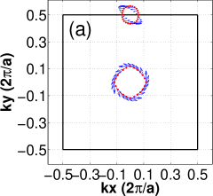
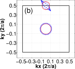
Figure 4: Spin texture on the (001) direction surface states near $\bar{\Gamma}$ and $\bar{X}$ point, (a) from the tight-binding model; (b) from the k$\cdot$p model results.

To understand the spin orientation on the surface states, we can construct the surface effective Hamiltonian at $\bar{\Gamma}$ and $\bar{X}$ points on the 2D projected surface BZ. On the 2D BZ, the little group is $C_{4v}$ at $\bar{\Gamma}$ point and $C_{2v}$ at $\bar{X}$ point. The surface states at these two points are transformed as the states with $j_{z}=\pm 3/2$ under the symmetry operation in the little group. Form the symmetry consideration, we can write down the effective Hamiltonian for the surface states at $\bar{\Gamma}$ and $\bar{X}$ points respectively:

1) At $\bar{\Gamma}$ point: The Hamiltonian satisfy the $C_{4v}$ symmetry and time-reversal symmetry must having the following form up to the third order of $k$:

$$H_{\bar{\Gamma}}^{ss}(k)=c_{0}k^{2}+\bigg{[}i(c_{1}k_{+}+c_{2}k_{+}^{2}k_{-}+c_{3}k_{-}^{3})\hat{\sigma}_{+}+h.c.\bigg{]},$$ (11)

in the basis of {$|j_{z}=\frac{3}{2}\rangle,|j_{z}=-\frac{3}{2}\rangle$}. Where $\hat{\sigma}_{\pm}=\hat{\sigma}_{x}\pm i\hat{\sigma}_{y}$, $k_{\pm}=k_{x}\pm ik_{y}$ and $k^{2}=k_{x}^{2}+k_{y}^{2}$. The parameters are listed in table.2

Here we should determine the spin operators $\hat{s}_{x,y,z}$ for the surface model Hamiltonian at $\bar{\Gamma}$ point . We start from the tight-binding Hamiltonian $H_{eff}$, which is written in the tight-binding basis space expanded by $d$ and $f$ orbitals located on Sm atoms. Based on this tight-binding model we can construct a thick slab terminated in the (001) direction and calculate the surface states $|\Psi_{\alpha}\rangle$, $\alpha=1,2$. The spin operator $\mathbf{\hat{S}}$ for this slab system can be easily written in the tight-binding basis. Then, we project the spin operator $\mathbf{\hat{S}}$ onto the surface states subspace. Finally, we find that the spin operators for surface states are

$$s_{x}^{\alpha\beta} = \langle\Psi_{\alpha}|\hat{S}_{x}|\Psi_{\beta}\rangle=0.0953\sigma_{x}^{\alpha\beta}$$

$$s_{y}^{\alpha\beta} = \langle\Psi_{\alpha}|\hat{S}_{y}|\Psi_{\beta}\rangle=-0.0953\sigma_{y}^{\alpha\beta}$$

$$s_{z}^{\alpha\beta} = \langle\Psi_{\alpha}|\hat{S}_{z}|\Psi_{\beta}\rangle=0.0638\sigma_{z}^{\alpha\beta}$$ (12)

The total angular momentum operators in the surface states subspace can also be calculated as $\hat{j}_{x}=-0.6648\hat{\sigma}_{x}$, $\hat{j}_{y}=0.6648\hat{\sigma}_{y}$ $\hat{j}_{z}=-0.5405\hat{\sigma}_{z}$.

In order to predict or understand properties of the surface states under the external magnetic field, we give the Zeeman coupling terms for surface states, which takes the following form

$$H_{\bar{\Gamma}}^{ss,Z}=\mu_{B}\sum_{\alpha,\beta}g_{\alpha\beta}{\hat{\sigma}}_{\alpha}B_{\beta},$$ (13)

which is obtained by projecting the $H_{Zeeman}=\frac{\mu_{B}}{\hbar}(\hat{\mathbf{L}}+2\hat{\mathbf{S}})\cdot\mathbf{B}$ term into the surface states subspace. Here $\hat{\mathbf{L}}$ and $\hat{\mathbf{S}}$ are the orbital angular momentum and spin operator of the slab system. The the non-zero matrix elements of the g factor matrix for surface states at $\bar{\Gamma}$ point are listed in table.2

2) At $\bar{X}$ point: As shown in Fig.(3), the Dirac cone has a good linear dispersion. The surface effective Hamiltonian which satisfying the $C_{2v}$ symmetry and time-reversal symmetry must have the following form up to the second order of $k$ in the basis of {$|j_{z}=\frac{3}{2}\rangle,|j_{z}=-\frac{3}{2}\rangle$},

$$H_{\bar{X}}^{ss}(\mathbf{k})=(\epsilon_{0}+a_{0}k^{2})\sigma_{0}+\big{[}i(a_{1}k_{+}+a_{2}k_{-})\hat{\sigma}_{+}+h.c.\big{]}.$$ (14)

The spin operators for surface states are

$$\hat{s}_{x}=0.0687\hat{\sigma}_{x};\;\hat{s}_{y}=-0.1223\hat{\sigma}_{y};\;\hat{s}_{z}=-0.1484\hat{\sigma}_{z}$$ (15)

The total angular momentum operators in the surface states subspace can also be calculated as $\hat{j}_{x}=-0.4201\hat{\sigma}_{x}$, $\hat{j}_{y}=0.7870\hat{\sigma}_{y}$ $\hat{j}_{z}=0.9309\hat{\sigma}_{z}$, The Zeeman term for surface states at $\bar{X}$ point is the same as Eq.(13) and the g factors are listed in table.2.

Table 2: Parameters for the surface states model. The unit of energy is eV and the unit of length is the lattice constant.

$H_{\bar{\Gamma}}^{ss}$	$c_{0}$	$c_{1}$	$c_{2}$	$c_{3}$
	0.64105	0.01524	1.1081	-0.0516
	$g_{xx}$	$g_{yy}$	$g_{zz}$
	-0.5695	0.5695	-0.4768
$H_{\bar{X}}^{ss}$	$a_{0}$	$a_{1}$	$a_{2}$	$\epsilon_{0}$
	0.011276	0.003059	-0.02322	0.008654
	$g_{xx}$	$g_{yy}$	$g_{zz}$
	-0.3514	0.6647	0.7825

CONCLUSIONS

To summarize, we have derived the model Hamiltonians around the three X points for the 3D TI SmB₆ based on the first principles results and the symmetry considerations. The bulk band structure, the surface states on (001) surface and the spin texture of the surface states can be well described by our model Hamiltonians. These effective Hamiltonians could facilitate further investigations of similar intriguing materials.

Acknowledgments This work was supported by the WPI Initiative on Materials Nanoarchitectonics, and Grant-in-Aid for Scientific Research under the Innovative Area "Topological Quantum Phenomena" (No.25103723), MEXT of Japan. H.M. Weng, Zhong Fang and X. Dai acknowledge the NSF of China and the 973 Program of China (No. 2011CBA00108 and No. 2013CB921700) for support.

References

- Qi and Zhang (2011) X.-L. Qi and S.-C. Zhang, Reviews of Modern Physics 83, 1057 (2011).
- Hasan and Kane (2010) M. Z. Hasan and C. L. Kane, Reviews of Modern Physics 82, 3045 (2010).
- Roushan et al. (2009) P. Roushan, J. Seo, C. V. Parker, Y. S. Hor, D. Hsieh, D. Qian, A. Richardella, M. Z. Hasan, R. J. Cava, and A. Yazdani, Nature 460, 1106 (2009).
- Alpichshev et al. (2010) Z. Alpichshev, J. G. Analytis, J.-H. Chu, I. R. Fisher, Y. L. Chen, Z. X. Shen, A. Fang, and A. Kapitulnik, Physical Review Letters 104, 016401 (2010).
- Zhang et al. (2009) T. Zhang, P. Cheng, X. Chen, J.-F. Jia, X. Ma, K. He, L. Wang, H. Zhang, X. Dai, Z. Fang, et al., Physical Review Letters 103, 266803 (2009).
- Xia et al. (2009) Y. Xia, D. Qian, D. Hsieh, L. Wray, A. Pal, H. Lin, A. Bansil, D. Grauer, Y. S. Hor, R. J. Cava, et al., Nature Physics 5, 398 (2009).
- Beidenkopf et al. (2011) H. Beidenkopf, P. Roushan, J. Seo, L. Gorman, I. Drozdov, Y. S. Hor, R. J. Cava, and A. Yazdani, Nature Physics 7, 939 (2011).
- Fu and Kane (2008) L. Fu and C. L. Kane, Physical Review Letters 100, 096407 (2008).
- Santos et al. (2010) L. Santos, T. Neupert, C. Chamon, and C. Mudry, Physical Review B 81, 184502 (2010).
- Qi et al. (2010) X.-L. Qi, T. L. Hughes, and S.-C. Zhang, Physical Review B 82, 184516 (2010).
- Moore (2010) J. E. Moore, Nature 464, 194 (2010).
- Dzero et al. (2009) M. Dzero, K. Sun, V. Galitski, and P. Coleman, Physical Review Letters 10, 106408 (2009).
- Dzero et al. (2012) M. Dzero, K. Sun, P. Coleman, and V. Galitski, Physical Review B 85, 045130 (2012).
- Alexandrov et al. (2013a) V. Alexandrov, M. Dzero, and P. Coleman, Physical Review Letters 111, 226403 (2013a).
- Ye et al. (2013) M. Ye, J. W. Allen, and K. Sun, arXiv.org p. 7191 (2013), eprint 1307.7191.
- Dzero and Galitski (2013) M. Dzero and V. Galitski, Journal of Experimental and Theoretical Physics 117, 499 (2013).
- Lu et al. (2013) F. Lu, J. Zhao, H. Weng, Z. Fang, and X. Dai, Physical Review Letters 110, 096401 (2013).
- Weng et al. (2014) H. Weng, J. Zhao, Z. Wang, Z. Fang, and X. Dai, Physical Review Letters 112, 016403 (2014).
- Deng et al. (2013) X. Deng, K. Haule, and G. Kotliar, Physical Review Letters 111, 176404 (2013).
- Alexandrov et al. (2013b) V. Alexandrov, M. Dzero, and P. Coleman, Physical Review Letters 111, 226403 (2013b).
- Legner et al. (2014) M. Legner, A. Ruegg, and M. Sigrist, Physical Review B 89, 085110 (2014).
- Werner and Assaad (2013) J. Werner and F. F. Assaad, Physical Review B 88, 035113 (2013).
- Frantzeskakis et al. (2013a) E. Frantzeskakis, N. de Jong, B. Zwartsenberg, Y. Huang, Y. Pan, X. Zhang, J. Zhang, F. Zhang, L. Bao, O. Tegus, et al., Physical Review X 3, 041024 (2013a).
- Wolgast et al. (2013) S. Wolgast, Ç. Kurdak, K. Sun, J. W. Allen, D.-J. Kim, and Z. Fisk, Physical Review B 88, 180405 (2013).
- Xu et al. (2013) N. Xu, X. Shi, P. K. Biswas, C. E. Matt, R. S. Dhaka, Y. Huang, N. C. Plumb, M. Radovic, J. H. Dil, E. Pomjakushina, et al., Physical Review B 88, 121102 (2013).
- Li et al. (2013) G. Li, Z. Xiang, F. Yu, T. Asaba, B. Lawson, P. Cai, C. Tinsman, A. Berkley, S. Wolgast, Y. S. Eo, et al., arXiv.org p. 5221 (2013), eprint 1306.5221.
- Neupane et al. (2013) M. Neupane, N. Alidoust, S. Y. Xu, T. Kondo, Y. Ishida, D. J. Kim, C. Liu, I. Belopolski, Y. J. Jo, T. R. Chang, et al., Nature Communications 4 (2013).
- Kim et al. (2013) D. J. Kim, S. Thomas, T. Grant, J. Botimer, Z. Fisk, and J. Xia, Nature Scientific Reports 3, 3150 (2013).
- Jiang et al. (2013) J. Jiang, S. Li, T. Zhang, Z. Sun, F. Chen, Z. R. Ye, M. Xu, Q. Q. Ge, S. Y. Tan, X. H. Niu, et al., Nature Communications 4, 3010 (2013).
- Thomas et al. (2013) S. Thomas, D. J. Kim, S. B. Chung, T. Grant, Z. Fisk, and J. Xia, arXiv.org p. 4133 (2013), eprint 1307.4133.
- Yee et al. (2013) M. M. Yee, Y. He, A. Soumyanarayanan, D.-J. Kim, Z. Fisk, and J. E. Hoffman, arXiv.org p. 1085 (2013), eprint 1308.1085.
- Denlinger et al. (2013a) J. D. Denlinger, J. W. Allen, J. S. Kang, K. Sun, J. W. Kim, J. H. Shim, B. I. Min, D.-J. Kim, and Z. Fisk, arXiv.org p. 6637 (2013a), eprint 1312.6637.
- Frantzeskakis et al. (2013b) E. Frantzeskakis, N. de Jong, B. Zwartsenberg, Y. K. Huang, Y. Pan, X. Zhang, J. X. Zhang, F. X. Zhang, L. H. Bao, O. Tegus, et al., Physical Review X 3, 4260431 (2013b).
- Ruan et al. (2014) W. Ruan, C. Ye, M. Guo, F. Chen, X. Chen, G.-M. Zhang, and Y. Wang, Physical Review Letters 112, 136401 (2014).
- Denlinger et al. (2013b) J. D. Denlinger, J. W. Allen, J.-S. Kang, K. Sun, B.-I. Min, D.-J. Kim, and Z. Fisk, arXiv.org p. 6636 (2013b), eprint 1312.6636.
- Beaurepaire et al. (1990) E. Beaurepaire, J. P. Kappler, and G. Krill, Physical Review B 41, 6768 (1990).
- Cohen et al. (1970) R. L. Cohen, M. Eibschutz, and K. W. West, Physical Review Letters 24, 383 (1970).
- Eibschutz et al. (1972) M. Eibschutz, R. L. Cohen, E. Buehler, and J. H. Wernick, Physical Review B 6, 18 (1972).
- Chazalviel et al. (1976) J. N. Chazalviel, M. Campagna, G. K. Wertheim, and P. H. Schmidt, Physical Review B 14, 4586 (1976).
- Kane and Mele (2005) C. L. Kane and E. J. Mele, Physical Review Letters 95, 146802 (2005).
- Fu and Kane (2006) L. Fu and C. Kane, Physical Review B 74, 195312 (2006).
- Deng et al. (2009) X. Deng, L. Wang, X. Dai, and Z. Fang, Physical Review B 79, 075114 (2009).
- Kotliar et al. (2006) G. Kotliar, S. Savrasov, K. Haule, V. Oudovenko, O. Parcollet, and C. Marianetti, Reviews of Modern Physics 78, 865 (2006).
- Kuneš et al. (2010) J. Kuneš, R. Arita, P. Wissgott, A. Toschi, H. Ikeda, and K. Held, Computer Physics Communications 181, 1888 (2010).
- Solovyev et al. (2007) I. V. Solovyev, Z. V. Pchelkina, and V. I. Anisimov, Physical Review B 75, 045110 (2007).
- Mostofi et al. (2008) A. A. Mostofi, J. R. Yates, Y.-S. Lee, I. Souza, D. Vanderbilt, and N. Marzari, Computer Physics Communications 178, 685 (2008).