A Poincaré-Bendixson theorem for meromorphic connections on Riemann surfaces

Abstract.

We shall prove a Poincaré-Bendixson theorem describing the asymptotic behavior of geodesics for a meromorphic connection on a compact Riemann surface. We shall also briefly discuss the case of non-compact Riemann surfaces, and study in detail the geodesics for a holomorphic connection on a complex torus.

1. Introduction

The main goal of this paper is to prove a Poincaré-Bendixson theorem describing the asymptotic behavior of geodesics for a meromorphic connection on a compact Riemann surface.

Roughly speaking (see Section 2 for more details), a meromorphic connection on a Riemann surface $S$ is a $\mathbb{C}$-linear operator $\nabla\colon\mathcal{T}(S)\to\mathcal{M}^{1}(S)\otimes\mathcal{T}(S)$, where $\mathcal{T}(S)$ is the space of holomorphic vector fields on $S$ and $\mathcal{M}^{1}(S)$ is the space of meromorphic 1-forms on $S$, satisfying a Leibniz rule $\nabla(\phi s)=\phi\nabla s+d\phi\otimes s$ for every $s\in\mathcal{T}(S)$ and every meromorphic function $\phi\in\mathcal{M}(S)$. Meromorphic connections are a classical subject, related for instance to linear differential systems (see, e.g., [IY08]); but in this paper we shall study them following a less classical point of view, introduced in [AT11].

A meromorphic connection $\nabla$ on a Riemann surface $S$ (again, see Section 2 for details) can be represented in local coordinates by a meromorphic 1-form; it turns out that the poles (and the associated residues) of this form do not depend on the coordinates but only on the connection. If $p\in S$ is not a pole, as for ordinary connections in differential geometry, it is possible to use $\nabla$ for differentiating along a direction $v\in T_{p}S$ any vector field $s$ defined along a curve in $S$ tangent to $v$, obtaining a tangent vector $\nabla_{v}s\in T_{p}S$. In particular, if $\sigma\colon(a,b)\to S$ is a smooth curve with image contained in the complement of the poles, it makes sense to consider the vector field $\nabla_{\sigma^{\prime}}\sigma^{\prime}$ along $\sigma$; and we shall say that $\sigma$ is a geodesic for $\nabla$ if $\nabla_{\sigma^{\prime}}\sigma^{\prime}\equiv O$.

As far as we know, geodesics for meromorphic connections in this sense were first introduced in [AT11]. As shown there, locally they behave as Riemannian geodesics of a flat metric; but their global behavior can be very different from the global behavior of Riemannian geodesics. Thus they are an interesting object of study per se; but they also have dynamical applications, in particular in the theory of local discrete holomorphic dynamical systems of several variables — explaining why we are particularly interested in their asymptotic behavior.

One of the main open problems in local dynamics of several complex variables is the understanding of the dynamics, in a full neighbourhood of the origin, of holomorphic germs tangent to the identity, that is of germs of holomorphic endomorphisms of $\mathbb{C}^{n}$ fixing the origin and with differential there equal to the identity. In dimension one, the Leau-Fatou flower theorem (see, e.g., [Aba10] or [Mil06]) provides exactly such an understanding; and building on this theorem Camacho ([Cam78]; see also [Shc82]) in 1978 has been able to prove that every holomorphic germ tangent to the identity in dimension one is locally topologically conjugated to the time-1 map of a homogeneous vector field. In other words, time-$1$ maps of homogeneous vector fields provide a complete list of models for the local topological dynamics of one-dimensional holomorphic germs tangent to the identity.

In recent years, many authors have begun to study the local dynamics of germs tangent to the identity in several complex variables; see, e.g., Écalle [Éca81a, Éca81b, Éca85], Hakim [Hak97, Hak98], Abate, Bracci, Tovena [Aba01, AT03, ABT04, AT11], Rong [Ron10], Molino [Mol09], Vivas [Viv11], Arizzi, Raissy [AR14], and others. A few generalizations to several variables of the Leau-Fatou flower theorem have been proved, but none of them was strong enough to be able to describe the dynamics in a full neighbourhood of the origin; furthermore, examples of unexpected phenomena not appearing in the one-dimensional case have been found. Thus it is only natural to try and study the dynamics of meaningful classes of examples, with the aim of extracting ideas applicable to a general setting; and Camacho’s theorem suggests that a particularly interesting class of examples is provided by time-1 maps of homogeneous vector fields. (Actually, the evidence collected so far strongly suggests that a several variable version of Camacho’s theorem might hold: generic germs tangent to the identity should be locally topologically conjugated to time-1 maps of homogeneous vector fields. But we shall not pursue this topic here.)

This is the approach initiated in [AT11]; and we discovered that there is a strong relationship between the dynamics of the time-1 map of homogeneous vector fields and the dynamics of geodesics for meromorphic connections on Riemann surfaces. To describe this relationship, we need to introduce a few notations and definitions.

Let $Q$ be a homogeneous vector field on $\mathbb{C}^{n}$ of degree $\nu+1\geq 2$. First of all, notice that the orbits of its time-1 map are contained in the real integral curves of $Q$; so we are interested in studying the dynamics of the real integral curves of the complex homogeneous vector field $Q$. (Actually, it turns out that complex integral curves of a homogeneous vector field are related to — classically studied— sections which are horizontal with respect to a meromorphic connection; see [AT11] for details.)

A characteristic direction for $Q$ is a direction $v\in\mathbb{P}^{n-1}(\mathbb{C})$ such that the complex line (the characteristic leaf) issuing from the origin in the direction $v$ is $Q$-invariant. An integral curve issuing from a point of a characteristic leaf stays in that leaf forever; so the dynamics in a characteristic leaf is one-dimensional, and thus completely known. In particular, if the vector field $Q$ is a multiple of the radial field (we shall say that $Q$ is dicritical) every direction is characteristic, the dynamics is one-dimensional and completely understood. So, we are mainly interested in understanding the dynamics of integral curves outside the characteristic leaves of non-dicritical vector fields.

Then in [AT11] we proved the following result:

Theorem 1.1 (Abate-Tovena [AT11]).

Let $Q$ be a non-dicritical homogeneous vector field of degree $\nu+1\geq 2$ in $\mathbb{C}^{n}$ and let $M_{Q}$ be the complement in $\mathbb{C}^{n}$ of the characteristic leaves of $Q$. Let $[\cdot]\colon\mathbb{C}^{n}\setminus\{O\}\to\mathbb{P}^{n-1}(\mathbb{C})$ denote the canonical projection. Then there exists a singular holomorphic foliation $\mathcal{F}$ of $\mathbb{P}^{n-1}(\mathbb{C})$ in Riemann surfaces, and a partial meromorphic connection $\nabla$ inducing a meromorphic connection on each leaf of $\mathcal{F}$, whose poles coincide with the characteristic directions of $Q$, such that the following hold:

1. if $\gamma\colon I\to M_{Q}$ is an integral curve of $Q$ then the image of $[\gamma]$ is contained in a leaf $S$ of $\mathcal{F}$ and it is a geodesic for $\nabla$ in $S$;

2. conversely, if $\sigma\colon I\to\mathbb{P}^{n-1}(\mathbb{C})$ is a geodesic for $\nabla$ in a leaf $S$ of $\mathcal{F}$ then there are exactly $\nu$ integral curves $\gamma_{1},\ldots,\gamma_{\nu}\colon I\to M_{Q}$ such that $[\gamma_{j}]=\sigma$ for $j=1,\ldots,\nu$.

Thanks to this result, we see that the study of integral curves for a homogeneous vector field in $\mathbb{C}^{n}$ is reduced to the study of geodesics for meromorphic connections on a Riemann surface $S$ (obtained as a leaf of the foliation $\mathcal{F}$).

In [AT11] the latter study has been carried out in the case $S=\mathbb{P}^{1}(\mathbb{C})$, which is the only case arising when $n=2$ (and indeed it has led to a fairly extensive understanding of the dynamics of homogeneous vector fields in $\mathbb{C}^{2}$, including the description of the dynamics in a full neighbourhood of the origin for a substantial class of examples); the main goal of this paper is to extend this study from $\mathbb{P}^{1}(\mathbb{C})$ to a generic compact Riemann surface, with the hope of applying in the future our results to the study of the dynamics of homogeneous vector fields in $\mathbb{C}^{n}$ with $n\geq 3$.

More precisely, we shall prove a Poincaré-Bendixson theorem (see Theorems 4.3 and 5.1) describing the $\omega$-limit set of the geodesics for a meromorphic connection on a generic compact Riemann surface. We recall that, in general, a “Poincaré-Bendixson theorem” is a result describing recurrence properties of a class of dynamical systems (see [Cie12] for a survey on the subject). An important ingredient in our proof will indeed be another Poincaré-Bendixson theorem, due to Hounie ([Hou81]), describing the minimal sets for smooth singular line fields on compact orientable surfaces (which in turn follows from a similar statement for smooth vector fields, see [Sch63]).

The paper is organized as follows. In Section 2 we collect all the preliminary results that we shall need. In Section 3 we generalize results obtained in [AT11] concerning geodesics for meromorphic connections on the Riemann sphere to geodesics for meromorphic connections on a generic compact Riemann surface. In Sections 4 and 5 we prove our main Theorems: we shall show that it is possible to see a geodesic for a meromorphic connection as part of an integral curve for a suitable line field on the surface, which, in a neighbourhood of the support of the geodesic, is singular exactly on the poles of the connection; then, thanks to the result of Hounie mentioned above, we shall be able to give a topological description of the possible minimal sets, and we shall conclude the proof by applying the theory developed in the previous sections. In Section 6 we shall briefly discuss what happens on non-compact Riemann surfaces. Finally, in Section 7 we present a detailed study of the geodesics for holomorphic connections on complex tori (the only compact Riemann surfaces admitting meromorphic connections without poles).

2. Preliminary notions

Throughout this paper we shall denote by $S$ a Riemann surface and by $p\colon TS\to S$ the tangent bundle on $S$. Furthermore, $\mathcal{O}_{S}$ will be the structure sheaf of $S$, i.e., the sheaf of germs of holomorphic functions on $S$, and $\mathcal{M}_{S}$ the sheaf of germs of meromorphic functions. $\mathcal{T}\mathcal{S}$ will denote the sheaf of germs of holomorphic sections of $TS$ and $\mathcal{M}_{TS}$ the sheaf of germs of its meromorphic sections. Finally, $\Omega^{1}_{S}$ will denote the sheaf of germs of holomorphic 1-forms, and $\mathcal{M}_{S}^{1}$ the sheaf of germs of meromorphic 1-forms.

We start recalling the definitions and the first properties of holomorphic and meromorphic connections on $p\colon TS\to S$. We refer to [AT11] and [IY08] for details.

Definition 2.1.   A holomorphic connection on the tangent bundle $p\colon TS\to S$ over a Riemann surface is a $\mathbb{C}$-linear map $\nabla\colon\mathcal{T}\mathcal{S}\to\Omega^{1}_{S}\otimes\mathcal{T}\mathcal{S}$ satisfying the Leibniz rule

$$\nabla(fs)=df\otimes s+f\nabla s$$

for all $s\in\mathcal{T}\mathcal{S}$ and $f\in\mathcal{O}_{S}$. We shall often write $\nabla_{u}s$ for $\nabla s(u)$.

A geodesic for a holomorphic connection $\nabla$ is a real curve $\sigma\colon I\to S$, with $I\subseteq\mathbb{R}$ an interval, such that $\nabla_{\sigma^{\prime}}\sigma^{\prime}\equiv 0$.

Let us see what this definition means in local coordinates. Given a holomorphic atlas $\{(U_{\alpha},z_{\alpha})\}$ on $S$, we denote by $\partial_{\alpha}:=\partial/\partial z_{\alpha}$ the induced local generator of $TS$ over $U_{\alpha}$. We shall always suppose that the $U_{\alpha}$’s are simply connected. On each $U_{\alpha}$ we can find a holomorphic 1-form $\eta_{\alpha}$ such that

$$\nabla\partial_{\alpha}=\eta_{\alpha}\otimes\partial_{\alpha}\;,$$

and we shall say that the form $\eta_{\alpha}$ represents the connection $\nabla$ on $U_{\alpha}$. In fact we see that, for a general section $s$ of $TS$, we can locally compute $\nabla s$ by representing $s|_{U_{\alpha}}$ as $s_{\alpha}\partial_{\alpha}$ for some holomorphic function $s_{\alpha}$ on $U_{\alpha}$ and writing

$$\nabla(s_{\alpha}\partial_{\alpha})=ds_{\alpha}\otimes\partial_{\alpha}+s_{\alpha}\nabla(\partial_{\alpha})=ds_{\alpha}\otimes\partial_{\alpha}+s_{\alpha}\eta_{\alpha}\otimes\partial_{\alpha}=(ds_{\alpha}+\eta_{\alpha})\otimes\partial_{\alpha}\;.$$

Definition 2.2.   Let $g$ be an Hermitian metric on $p\colon TS\to S$. We say that a connection $\nabla$ on $TS$ is adapted to, or compatible with, the metric $g$ if

$$d\langle R,T\rangle=\langle\nabla R,T\rangle+\langle R,\overline{\nabla}T\rangle$$

for every pair of smooth vector fields $R$, $T$, that is if

$$X\langle R,T\rangle=\langle\nabla_{X}R,T\rangle+\langle R,\nabla_{\bar{X}}T\rangle$$

for every triple of smooth vector fields $X$, $R$ and $T$ on $S$.

It is known that it is possible to associate to any Hermitian metric a (not necessarily holomorphic) connection on the tangent bundle adapted to it, the Chern connection. Locally, it is also possible to solve the converse problem, i.e., to construct local metrics adapted to a given holomorphic connection on $TS$. To do this, it is convenient to consider the local real function $n_{\alpha}\colon U_{\alpha}\to\mathbb{R}^{+}$ given by

$$n_{\alpha}(p)=g_{p}(\partial_{\alpha},\partial_{\alpha})\;.$$

It is straightforward to see that $n_{\alpha}$ is a smooth function and, conversely, we see that the function $n_{\alpha}$ uniquely determines the metric on $U_{\alpha}$.

With these notations in place it is not difficult to see that the compatibility of a metric $g$ with a holomorphic connection $\nabla$ on the domain $U_{\alpha}$ of a local chart is equivalent to

(2.1) $$\partial n_{\alpha}=n_{\alpha}\eta_{\alpha}\;.$$

Equation (2.1) can actually be solved:

Proposition 2.1 ([AT11], Proposition 1.1).

Let $\nabla\colon\mathcal{T}\mathcal{S}\to\Omega^{1}_{S}\otimes\mathcal{T}\mathcal{S}$ be a holomorphic connection on a Riemann surface $S$. Let $\left(U_{\alpha},z_{\alpha}\right)$ be a local chart for $S$ and let $\eta_{\alpha}\in\Omega^{1}_{S}(U_{\alpha})$ be the 1-form representing $\nabla$ on $U_{\alpha}$. Given a holomorphic primitive $K_{\alpha}$ of $\eta_{\alpha}$ on $U_{\alpha}$, then

$$n_{\alpha}=\exp(2\mathrm{Re}\,K_{\alpha})=\exp(K_{\alpha}+\bar{K_{\alpha}})$$

is a positive solution of (2.1).

Conversely, if $n_{\alpha}$ is a positive solution of (2.1) then for any $z_{0}\in U_{\alpha}$ and any simply connected neighbourhood $U\subseteq U_{\alpha}$ of $z_{0}$ there exists a holomorphic primitive $K_{\alpha}\in\mathcal{O}(U)$ of $\eta_{\alpha}$ over $U$ such that $n_{\alpha}=\exp(2\mathrm{Re}\,K_{\alpha})$ in U. Furthermore, $K_{\alpha}$ is unique up to a purely imaginary additive constant.

Finally, two (local) solutions of (2.1) differ (locally) by a positive multiplicative constant.

Remark 2.1.  It is important to notice that Proposition 2.1 gives only local metrics adapted to $\nabla$; a global metric adapted to $\nabla$ might not exist (see [AT11, Proposition 1.2]).

So we can associate to a holomorphic connection $\nabla$ a conformal family of compatible local metrics. It turns out (see [AT11]) that these local metrics are locally isometric to the Euclidean metric on $\mathbb{C}$. In fact, given any holomorphic primitive $K_{\alpha}$ of $\eta_{\alpha}$, let the function $J_{\alpha}\colon U_{\alpha}\to\mathbb{C}$ be a holomorphic primitive of $\exp({K_{\alpha}})$. We immediately remark that $J_{\alpha}$ actually exists, because $U_{\alpha}$ is simply connected, and that it is locally invertible, because $J_{\alpha}^{\prime}=\exp({K_{\alpha}})$. In the following Proposition we summarize the main properties of $J_{\alpha}$.

Proposition 2.2 ([AT11]).

Let $\nabla\colon\mathcal{T}\mathcal{S}\to\Omega^{1}_{S}\otimes\mathcal{T}\mathcal{S}$ be a holomorphic connection on a Riemann surface $S$. Let $\left(U_{\alpha},z_{\alpha}\right)$ be a local chart for $S$ with $U_{\alpha}$ simply connected, $\eta_{\alpha}$ the 1-form representing $\nabla$ on $U_{\alpha}$, and $K_{\alpha}$ a holomorphic primitive of $\eta_{\alpha}$ on $U_{\alpha}$. Then every primitive $J_{\alpha}\colon U_{\alpha}\to\mathbb{C}$ of $\exp(K_{\alpha})$ is a local isometry between $U_{\alpha}$, endowed with the metric represented by $n_{\alpha}=\exp(2\mathrm{Re}\,K_{\alpha})$, and $\mathbb{C}$, endowed with the Euclidean metric. In particular, every local metric adapted to $\nabla$ is flat, that is its Gaussian curvature vanishes identically.

Moreover, a smooth curve $\sigma\colon I\to{U_{\alpha}}$ is a geodesic for $\nabla$ if and only if there are two constants $c_{0}$ and $w_{0}\in\mathbb{C}$ such that $J_{\alpha}(\sigma(t))=c_{0}t+w_{0}$. In particular, the geodesic with $\sigma(0)=z_{0}$ and $\sigma^{\prime}(0)=v_{0}\in\mathbb{C}^{*}$ is given by

(2.2) $$\sigma(t)=J_{\alpha}^{-1}\left(c_{0}t+J_{\alpha}(z_{0})\right)\;,$$

where $c_{0}=\exp\left({K_{\alpha}}(z_{0})\right)v_{0}$ and $J_{\alpha}^{-1}$ is the analytic continuation of the local inverse of $J_{\alpha}$ near $J_{\alpha}(z_{0})$ such that $J_{\alpha}^{-1}\left(J_{\alpha}(z_{0})\right)=z_{0}$.

Finally, a curve $\sigma\colon[0,\varepsilon)\to U_{\alpha}$ is a geodesic for $\nabla$ if and only if

(2.3) $$\sigma^{\prime}(t)=\exp\left(-{K_{\alpha}}(\sigma(t))\right)\exp\left({K_{\alpha}}(\sigma(0))\right)\sigma^{\prime}(0)\;,$$

if and only if

(2.4) $$J_{\alpha}(\sigma(t))=\exp\left({K_{\alpha}}(\sigma(0))\right)\sigma^{\prime}(0)t+J_{\alpha}(\sigma(0)).$$

Remark 2.2.   Another consequence of the existence of a conformal family of local metrics adapted to $\nabla$ is that we can introduce on each tangent space $T_{p}S$ a well-defined notion of angle between tangent vectors, clearly independent of the particular local metric used to compute it.

We shall now give the official definition of meromorphic connection.

Definition 2.3.   A meromorphic connection on the tangent bundle $p\colon TS\to S$ of a Riemann surface $S$ is a $\mathbb{C}$-linear map $\nabla\colon\mathcal{M}_{TS}\to\mathcal{M}^{1}_{S}\otimes_{\mathcal{M}(S)}\mathcal{M}_{TS}$ satisfying the Leibniz rule

$$\nabla(\tilde{f}\tilde{s})=d\tilde{f}\otimes\tilde{s}+\tilde{f}\nabla\tilde{s}$$

for all $\tilde{s}\in\mathcal{M}_{TS}$ and $\tilde{f}\in\mathcal{M}_{S}$.

It is easy to see that on a local chart $(U_{\alpha},z_{\alpha})$ a meromorphic connection is represented by a meromorphic 1-form, that we continue to call $\eta_{\alpha}$, such that

$$\nabla(\partial_{\alpha})=\eta_{\alpha}\otimes\partial_{\alpha}$$

and so

$$\nabla(\tilde{s})=\nabla(\tilde{s}_{\alpha}\partial_{\alpha})=(d\tilde{s}_{\alpha}+\eta_{\alpha})\otimes\partial_{\alpha}$$

for every local meromorphic section $\tilde{s}|_{U_{\alpha}}=\tilde{s_{\alpha}}\partial_{\alpha}$ on $U_{\alpha}$, exactly as it happens for holomorphic connections.

In particular, all the forms $\eta_{\alpha}$’s are holomorphic if and only if $\nabla$ is a holomorphic connection. More precisely, if we say that $p\in S$ is a pole for a meromorphic connection $\nabla$ if $p$ is a pole of $\eta_{\alpha}$ for some (and hence any) local chart $U_{\alpha}$ at $p$, then $\nabla$ is a holomorphic connection on the complement $S^{0}$ of the poles of $\nabla$ in $S$.

This allows to define geodesics for a meromorphic connections as we did for holomorphic connections.

Definition 2.4.  A geodesic for a meromorphic connection $\nabla$ on $p\colon TS\to S$ is a real curve $\sigma\colon I\to S^{0}$, with $I\subseteq\mathbb{R}$ an interval, such that $\nabla_{\sigma^{\prime}}\sigma^{\prime}\equiv 0$.

The following definition will be of primary importance in the sequel.

Definition 2.5.  The residue $\mathrm{Res}_{p}\nabla$ of a meromorphic connection $\nabla$ at a point $p\in S$ is the residue of any 1-form $\eta_{\alpha}$ representing $\nabla$ on a local chart $(U_{\alpha},z_{\alpha})$ at $p$. Clearly, $\mathrm{Res}_{p}\nabla\neq 0$ only if $p$ is a pole of $\nabla$.

It is easy to see that the residue of a meromorphic connection at a point $p\in S$ is well defined, i.e., it does not depend on the particular chart $U_{\alpha}$. Moreover, by the Riemann-Roch formula, the sum of the residues of a meromorphic connection $\nabla$ is independent from the particular connection, as stated in the following classical Theorem (see [IY08] for a proof).

Theorem 2.1.

Let $S$ be a compact Riemann surface and $\nabla$ a meromorphic connection on $p\colon TS\to S$. Then

(2.5) $$\sum_{p\in S}\mathrm{Res}_{p}\nabla=-\chi_{S}\;,$$

where $\chi_{S}$ is the Euler characteristic of $S$.

Our main result is a classification of the possible $\omega$-limit sets for the geodesics of meromorphic connections on the tangent bundle of a compact Riemann surface. We recall that the $\omega$-limit set $\omega(\sigma)$ of a curve $\sigma\colon[0,\varepsilon)\to S^{0}$ is given by the points $p$ of $S$ for which there exists a sequence $\{t_{n}\}$, with $t_{n}\to\varepsilon$, such that $\sigma(t_{n})\to p$. It is easy to see that

$$\omega(\sigma)=\bigcap_{\varepsilon^{\prime}<\varepsilon}\overline{\{\sigma(t)\colon t>\varepsilon^{\prime}\}}.$$

The main part of the proof will consist in extending the tangent field of the geodesic to a smooth line field (a rank-1 real foliation) on $S$, singular only on the poles of the connection. Then we shall be able to use the following theorem by Hounie ([Hou81]) to study the minimal sets of this line field, where a minimal set for a line field $\Lambda$ is a closed, non-empty, $\Lambda$-invariant subset of $S$ without proper subsets having the same properties:

Theorem 2.2 (Hounie [Hou81]).

Let $S$ be a compact connected two-dimensional smooth real manifold (e.g., a Riemann surface) and let $\Lambda$ be a smooth line field with singularities on $S$. Then a $\Lambda$-minimal set $\Omega$ must be one of the following:

1. a singularity of $\Lambda$;

2. a closed integral curve of $\Lambda$, homeomorphic to $S^{1}$;

3. all of $S$, and in this case $\Lambda$ is equivalent to an irrational line field on the torus (i.e., there exists a homeomorphism $\phi\colon S\to T$ between $S$ and a torus $T$ transforming the given foliation into one induced by an irrational line field).

3. Meromorphic connections on the tangent bundle

In this section, we study in more detail geodesics for meromorphic connections on the tangent bundle of a compact Riemann surface. In particular, we extend results contained in Section 4 of [AT11] from $\mathbb{P}^{1}(\mathbb{C})$ to the case of a generic compact Riemann surface $S$.

To do so, we start introducing the following definitions/notations.

Definition 3.1.   Let $S$ be a compact Riemann surface. Let $\nabla$ be a meromorphic connection on $TS$ and let $S^{0}\subseteq S$ be the complement of the poles.

• A geodesic ($n$-)cycle is the union of $n$ geodesic segments $\sigma_{j}\colon[0,1]\to S^{0}$, disjoint except for the conditions $\sigma_{j}(0)=\sigma_{j-1}(1)$ for $j=2,\ldots,n$ and $\sigma_{1}(0)=\sigma_{n}(1)$. The points $\sigma_{j}(0)$ will be called vertices of the geodesic cycle.

• A ($m$-)multicurve is a union of $m$ disjoint geodesic cycles. A multicurve will be said to be disconnecting if it disconnects $S$, non-disconnecting otherwise.

• A part $P$ is the closure of a connected open subset of $S$ whose boundary is a multicurve $\gamma$. A component $\sigma$ of $\gamma$ is surrounded if the interior of $P$ contains both sides of a tubular neighbourhood of $\sigma$ in $S$; it is free otherwise. The filling $\hat{P}$ of a part $P$ is the compact surface obtained by glueing a disk along each of the free components of $\gamma$, and not removing any of the surrounded components of $\gamma$.

We remark that a part may be all of $S$, when the associated multicurve is non-disconnecting (which is equivalent to saying that the multicurve has no free components). Moreover, we see that every disconnecting multicurve contains the boundary of a part $P\varsubsetneq S$.

As recalled in the previous section, we can associate to a meromorphic connection $\nabla$ conformal families of local metrics on the regular part $S^{0}\subseteq S$ of the Riemann surface, and we have a well-defined notion of angle between tangent vectors. In particular, it makes sense to speak of the external angle $\epsilon$ at a vertex $\sigma_{j}(0)$ of a geodesic cycle as the angle between the tangent vectors $\sigma^{\prime}_{j-1}(1)$ and $\sigma^{\prime}_{j}(0)$; by definition, $\epsilon\in(-\pi,\pi)$.

Again using the conformal families of local metric it is possible to define the geodesic curvature $k_{g}$ of a curve contained in $S^{0}$. In particular, if $p\in S$ is a pole of $\nabla$ and $\tau$ is a small (clockwise) circle around $p$, not containing other poles, we have

(3.1) $$\int_{\tau}k_{g}=-2\pi(1+\mathrm{Re}\,\mathrm{Res}_{p}(\nabla))\;;$$

see [AT11, Theorem 4.1].

With all these ingredients at our disposal, it becomes natural to try and apply a Gauss-Bonnet Theorem to study the relation between the residues of the connection $\nabla$ in a part $P$ of $S$, the external angles at the vertices of the multicurve bounding $P$ and the topology of $S$ (cp. [AT11, Theorem 4.1]).

Theorem 3.1.

Let $\nabla$ be a meromorphic connection on a compact Riemann surface $S$, with poles $\{p_{1},\dots,p_{r}\}$ and set $S^{0}:=S\setminus\{p_{1},\dots,p_{r}\}$. Let $P$ be a part of $S$ whose boundary multicurve $\gamma\subset S^{0}$ has $m_{f}\geq 1$ free components, positively oriented with respect to $P$. Let $z_{1},\dots,z_{s}$ denote the vertices of the free components of $\gamma$, and $\varepsilon_{j}\in(-\pi,\pi)$ the external angle at $z_{j}$. Suppose that $P$ contains the poles $\{p_{1},\dots,p_{g}\}$ and denote by $g_{\hat{P}}$ the genus of the filling $\hat{P}$ of $P$. Then

(3.2) $$\sum_{j=1}^{s}\varepsilon_{j}=2\pi\left(2-m_{f}-2g_{\hat{P}}+\sum_{j=1}^{g}\mathrm{Re}\,\mathrm{Res}_{p_{j}}(\nabla)\right)\;.$$

Proof.  For $j=1,\ldots,g$ let $\tau_{j}$ be a small clockwise circle bounding a disk in $P$ centered at $p_{j}$, and let $k_{g}^{j}$ be the geodesic curvature of $\tau_{j}$.

Applying the Gauss-Bonnet Theorem as in [AT11, Theorem 4.1] to the complement $P^{0}$ in $P$ of the small disks bounded by $\tau_{1},\ldots,\tau_{g}$ we find that

(3.3) $$\sum_{j=1}^{g}\int_{\tau_{j}}k_{g}^{j}+\sum_{j=1}^{s}\varepsilon_{j}=2\pi\chi_{P^{0}}=2\pi(2-m_{f}-g-2g_{\hat{P}})\;.$$

But from (3.1) we get

(3.4) $$\sum_{j=1}^{g}\int_{\tau_{j}}k_{g}^{j}=-2\pi g-2\pi\sum_{j=1}^{g}\mathrm{Re}\,\mathrm{Res}_{p_{j}}(\nabla)\;.$$

Comparing (3.3) and (3.4) we get the assertion. $\Box$

Remark 3.1.  When the multicurve $\gamma$ does not disconnect $S$ then Theorem 3.1 reduces to Theorem 2.1. Indeed, in this case $\gamma$ has no free components, and thus (3.2) becomes

$$0=2\pi\left(2-2g_{S}+\sum_{j=1}^{g}\mathrm{Re}\,\mathrm{Res}_{p_{j}}(\nabla)\right)\;,$$

which is equivalent to (2.5).

In the next two Corollaries we highlight what happens when the disconnecting multicurve is made up by a single geodesic or by a single geodesic cycle composed by two geodesics (cp. [AT11, Corollaries 4.2 and 4.3]).

Corollary 3.1 (One disconnecting geodesic).

Let $\nabla$ be a meromorphic connection on a compact Riemann surface $S$, with poles $\{p_{1},\dots,p_{r}\}$ and set $S^{0}:=S\setminus\{p_{1},\dots,p_{r}\}$. Let $\sigma$ be a disconnecting geodesic $1$-cycle. Let $P$ be one of the two parts in which $S$ is disconnected by $\sigma$ and $\varepsilon\in(-\pi,\pi)$ the unique external angle of $\sigma$. Then

$$\varepsilon=2\pi\left(1-2g_{\hat{P}}+\sum_{p_{j}\in P}\mathrm{Re}\,\mathrm{Res}_{p_{j}}(\nabla)\right)\;.$$

In particular,

$$\sum_{p_{j}\in P}\mathrm{Re}\,\mathrm{Res}_{p_{j}}(\nabla)\in(-3/2+2g_{\hat{P}},-1/2+2g_{\hat{P}})\;.$$

Corollary 3.2 (Two geodesics whose union disconnects $S$).

Let $\nabla$ be a meromorphic connection on a compact Riemann surface $S$, with poles $\{p_{1},\dots,p_{r}\}$ and set $S^{0}:=S\setminus\{p_{1},\dots,p_{r}\}$. Let $\gamma$ be a disconnecting geodesic $2$-cycle. Let $P$ be one of the two parts in which $S$ is disconnected by $\gamma$, and $\varepsilon_{0}$,  $\varepsilon_{1}\in(-\pi,\pi)$ the two external angles of $\gamma$. Then

$$\varepsilon_{0}+\varepsilon_{1}=2\pi\left(1-2g_{\hat{P}}+\sum_{p_{j}\in P}\mathrm{Re}\,\mathrm{Res}_{p_{j}}(\nabla)\right)\;,$$

and hence

$$\sum_{p_{j}\in P}\mathrm{Re}\,\mathrm{Res}_{p_{j}}(\nabla)\in(-2+2g_{\hat{P}},2g_{\hat{P}})\;.$$

Remark 3.2.   In particular, a part of $S$ bounded by a disconnecting $1$-cycle or by a disconnecting $2$-cycle must necessarily contain a pole, because $0\notin(-2+2g_{\hat{P}},2g_{\hat{P}})$.

In the following we shall need to consider closed geodesics and periodic geodesics for a meromorphic connection.

Definition 3.2.  A geodesic $\sigma\colon[0,l]\to S$ is closed if $\sigma(l)=\sigma(0)$ and $\sigma^{\prime}(l)$ is a positive multiple of $\sigma^{\prime}(0)$; it is periodic if $\sigma(l)=\sigma(0)$ and $\sigma^{\prime}(l)=\sigma^{\prime}(0)$.

By Corollary 3.1 we immediately see that a disconnecting geodesic 1-cycle $\sigma$ is a closed geodesic if and only if for every part $P$ of $S$ bounded by $\sigma$ we have

(3.5) $$\sum_{p_{j}\in P}\mathrm{Re}\,\mathrm{Res}_{p_{j}}(\nabla)=-1+2g_{\hat{P}}\;.$$

Contrarily to the Riemannian case, closed geodesics are not necessarily periodic; for examples (and more) in the Riemann sphere see [AT11], and for examples on a complex torus see Section 7.

4. $\omega$-limits sets of geodesics

In this section we prove our main Theorem, the classification of the possible $\omega$-limit sets of geodesics for a meromorphic connection on a compact Riemann surface. The main idea will be to see a not self-intersecting geodesic $\sigma$ as part of an integral curve of a suitable line field $\Lambda$ on $S$, and then to apply Theorem 2.2 to get some information about the minimal sets for $\Lambda$ contained in the $\omega$-limit set of $\sigma$. Then we shall use these information to discuss the shape of the $\omega$-limit set itself.

Let us start by studying the local structure of the $\omega$-limit set of a not self-intersecting geodesic $\sigma$.

Proposition 4.1.

Let $S$ be a Riemann surface, $\nabla$ a meromorphic connection on $S$, and $S^{0}$ the complement of the poles for $\nabla$. Let $\sigma\colon I\to S^{0}$ be a maximal not self-intersecting geodesic for $\nabla$ and denote by $W$ its $\omega$-limit set. Let $z\in W\cap S^{0}$. Then:

1. there exists a unique direction $v$ at $z$ such that for every sequence $\{z_{n}\}\subset\sigma(I)$ with $z_{n}\to z$ the directions $\sigma^{\prime}(z_{n})$ converge to $v$; moreover, the image of the maximal geodesic $\sigma_{z}$ issuing from $z$ in the direction $v$ is contained in $W$;

2. if $W$ contains a curve $\tau$ passing through $z$ transversal to $\sigma_{z}$ then $z\in\mathring{W}$;

3. if $z\in\partial W$ then $\sigma_{z}$ is the unique geodesic segment through $z$ contained in $W$.

Proof.  (i) The existence of $v$ follows from the fact that $\sigma$ does not self-intersect. Using a local isometry $J$ defined in a neighbourhood of $z$ transforming geodesic segments in Euclidean segments we immediately see that the image of the geodesic segment issuing from $z$ in the direction $v$ must be contained in $W$, and the maximality follows from the maximality of $\sigma$.

(ii) Up to using a local isometry $J$ we can assume that all geodesic segments in a neighbourhood of $z$ are Euclidean segments.

Consider a point $z^{\prime}\neq z$ belonging to $\tau$. Since $z^{\prime}\in W\subset S^{0}$, (i) gives us a geodesic segment $\sigma_{z^{\prime}}$ through $z^{\prime}$ contained in $W$. Notice that $\sigma_{z^{\prime}}\neq\tau$ as soon as $z^{\prime}$ is close enough to $z$. In fact, since we have segments of $\sigma$ accumulating $\sigma_{z}$, the segments of $\sigma$ accumulating $\sigma_{z^{\prime}}$ cannot converge to $\tau$ without forcing $\sigma$ to self-intersect, impossible. The mapping $z^{\prime}\mapsto\sigma_{z^{\prime}}$ is continuous, again because $\sigma$ cannot self-intersect; thus the geodesic segments $\sigma_{z^{\prime}}$ fill an open neighbourhood of $z$ contained in $W$, and $z\in\mathring{W}$ as claimed.

(iii) It immediately follows from (ii). $\Box$

Definition 4.2.  Let $S$ be a Riemann surface, $\nabla$ a meromorphic connection on $S$, and $S^{0}$ the complement of the poles of $\nabla$. Let $\sigma\colon I\to S^{0}$ be a maximal not self-intersecting geodesic for $\nabla$, with $\omega$-limit $W\subseteq S$. Given $z\in W\cap S^{0}$, the maximal geodesic $\sigma_{z}$ given by Proposition 4.1.(i) issuing from $z$ and contained in $W$ is the distinguished geodesic issuing from $z$.

The following two lemmas contain basic properties of distinguished geodesics.

Lemma 4.1.

Let $S$ be a Riemann surface, $\nabla$ a meromorphic connection on $S$, and $S^{0}$ the complement of the poles of $\nabla$. Let $\sigma\colon I\to S^{0}$ be a maximal not self-intersecting geodesic for $\nabla$, with $\omega$-limit $W\subseteq S$. Let $\sigma_{z}$ be the distinguished geodesic issuing from $z\in W\cap S^{0}$. Then either $\sigma_{z}=\sigma$ or $\sigma$ does not intersect $\sigma_{z}$.

Proof.  If $\sigma$ intersects $\sigma_{z}$, either $\sigma=\sigma_{z}$ or the intersection is transversal; but $\sigma$ accumulates $\sigma_{z}$, and thus in the latter case $\sigma$ must self-intersect, contradiction. $\Box$

Lemma 4.2.

Let $S$ be a Riemann surface, $\nabla$ a meromorphic connection on $S$, and $S^{0}$ the complement of the poles of $\nabla$. Let $\sigma\colon I\to S^{0}$ be a maximal not self-intersecting geodesic for $\nabla$, with $\omega$-limit $W\subseteq S$. Assume there exists a closed distinguished geodesic $\alpha\subseteq W$. Then $W=\alpha$.

Proof.  If $\alpha=\sigma$ then the assertion is trivial; so by the previous lemma we can assume that $\sigma$ does not intersect $\alpha$.

For each $w\in\alpha$ we can find a neighbourhood $A_{w}\subset S^{0}$ of $w$, contained in a tubular neighbourhood of $\alpha$, and an isometry $J_{w}\colon A_{w}\to B_{w}$ such that:

• $B_{w}$ is a quadrilateral containing the origin, with two opposite sides parallel to the imaginary axis;

• $J_{w}(w)=O$ and $J_{w}(\alpha\cap A_{w})$ is the intersection of $B_{w}$ with the real axis;

• the $J_{w}$-images of the connected components of the intersection of $\sigma$ with $A_{w}$ contained in the lower half-plane intersect both vertical sides of $B_{w}$ and accumulate the real axis (this can be achieved using Proposition 4.1.(i)).

By compactness, we can cover $\alpha$ with finitely many $A_{w_{0}},\ldots,A_{w_{r}}$ of such neighbourhoods; furthermore, we can also assume that each $A_{w_{j}}$ intersects only $A_{w_{j-1}}$ and $A_{w_{j+1}}$, with the usual convention $w_{-1}=w_{r}$ and $w_{r+1}=w_{0}$; let $A=A_{0}\cup\cdots\cup A_{r}$. Furthermore, since $A$ is contained in a tubular neighbourhood of $\alpha$ and $S$ is orientable, $A\setminus\alpha$ has exactly two connected components; and we can assume that the segments of $\sigma$ mapped by the $J_{w_{j}}$ in the lower half-plane (and thus accumulating $\alpha$) are all contained in the same connected component of $A\setminus\alpha$.

Let $\tau$ be the segment of geodesic issuing from $w_{0}$ such that $J_{w_{0}}(\tau)$ is the intersection of $B_{w_{0}}$ with the negative imaginary axis. Denote by $\{z_{j}\}$ the infinitely many intersections of $\sigma$ with $\tau$, accumulating $w_{0}$. Again by compactness, we can assume that if we follow $\sigma$ starting from a $z_{1}$ close enough to $w_{0}$ we stay in $A$ until we get to the next intersection $z_{2}$. Furthermore, by property (c) the segment $\sigma_{1}$ of $\sigma$ from $z_{1}$ to $z_{2}$ must intersects all $A_{w_{k}}$’s either in clockwise or in counter-clockwise order. Let $D\subset A$ denote the domain bounded by $\alpha$, the geodesic segment $\sigma_{1}$ and the geodesic segment of $\tau$ from $z_{1}$ to $z_{2}$.

Assume first that $z_{2}$ is closer to $w_{0}$ than $z_{1}$. In this case, if we follow $\sigma$ starting from $z_{2}$ property (c) forces $\sigma$ to remain inside $D$ because it cannot intersect itself nor $\alpha$. Furthermore, property (c) again implies that the next intersection $z_{3}$ should be closer to $w_{0}$ than $z_{2}$. We can then repeat the argument, and we find that successive intersections of $\sigma$ with $\tau$ monotonically converge to $w_{0}$. This implies that $\sigma$ accumulates $\alpha$ and nothing else, that is $W=\alpha$ as claimed.

If instead $z_{2}$ is farther away from $w_{0}$ than $z_{1}$, if we follow $\sigma$ starting from $z_{2}$ we may possibly leave $A$; but since $\sigma$ accumulates $w_{0}$ we must sooner or later get back to $D$, and the only way is intersecting $\tau$ in a point $z_{3}$ between $z_{1}$ and $z_{2}$. But now following $\sigma$ starting from $z_{3}$ we are forced to stay into $D$ until we intersect $\tau$ in a point $z_{4}$ necessarily closer to $w_{0}$ than $z_{1}$ — and a fortiori closer than $z_{3}$. We can then repeat the previous argument using $z_{3}$ and $z_{4}$ instead of $z_{1}$ and $z_{2}$ to get again the assertion. $\Box$

The main tool for the study of the global behavior of not self-intersecting geodesics is the following Theorem, providing a smooth line field $\Lambda$ such that $\sigma$ is (part of) an integral curve of $\Lambda$.

Theorem 4.1.

Let $S$ be a Riemann surface and $\nabla$ a meromorphic connection on $S$, with poles $p_{1},\dots,p_{r}\in S$. Let $S^{0}=S\setminus\{p_{1},\dots,p_{r}\}$. Let $\sigma\colon I\to S^{0}$ be a geodesic for $\nabla$ without self-intersections, maximal in both forward and backward time. Then there exists a smooth line field $\Lambda$ with singularities on $S$ which has $\sigma$ as integral curve and, in a neighbourhood of $\sigma$, is singular exactly on the poles of $\nabla$. Furthermore, the $\omega$-limit $W$ of $\sigma$ is $\Lambda$-invariant, and $\Lambda|_{W}$ is uniquely determined.

Proof.  If $A\subset S^{0}$ is open, simply connected and small enough, we can find a metric $g$ on $A$ compatible with $\nabla$ and an isometry $J$ between $A$ endowed with $g$ and an open set in $\mathbb{C}$ endowed with the euclidean metric; $g$ is unique up to a positive multiple (see Propositions 2.1 and 2.2).

We consider an open cover $\mathcal{A}=\{A_{i}\}$ of $S^{0}$ with the following properties:

1. $\mathcal{A}$ is locally finite;

2. each $A_{i}$ is endowed with a metric $g_{i}$ compatible with $\nabla$, and with an isometry $J_{i}\colon A_{i}\to B_{i}\subseteq\mathbb{C}$, with $B_{i}$ convex;

3. if $\sigma$ intersects $A_{i}$ then the angle between any pair of lines in $\mathbb{C}\supset B_{i}$ containing a component (which necessarily is a line segment) of the $J_{i}$-image of $\sigma$ is less than $\frac{\pi}{8}$. This can be achieved thanks to the smooth dependence of the solution of the geodesic equation from the initial conditions and the fact that the isometry is smooth.

We shall start building a line field on every open set $A_{i}$ of $\mathcal{A}$. Then we shall show how to use them to find a global line field $\Lambda$ on $S^{0}$ having $\sigma$ as integral curve, and finally we shall extend $\Lambda$ to all of $S$.

Let us then choose an open set $A\in\mathcal{A}$, together with its image $B$. We shall now construct a smooth flow of curves in $B$ that will correspond to a smooth flow of curves, and so to a line field, in $A$.

If $\sigma$ does not cross $A$, we put on $B$ any smooth vector field which is never zero and consider its associated (regular) foliation.

If $\sigma$ crosses $A$, we consider the segments $\sigma_{n}\subset B$ which are the images of the connected components of the intersection of $\sigma$ with $A$ (recall that $J$ sends geodesics segments in $A$ to Euclidean segments in $B$). By our assumption on $A$, the angle between $\sigma_{i}$ and $\sigma_{j}$ is bounded by $\frac{\pi}{8}$ for every pair $(i,j)$.

By the convexity of $B$ and the maximality of $\sigma$, the $\sigma_{n}$’s subdivide $B$ in connected components. We describe now how to costruct the flow in all these components.

1. If a connected component $C$ is open and its boundary (in $B$) consists of a unique $\sigma_{0}$, then we define our flow on $C$ by means of lines parallel to $\sigma_{0}$ and take the associated line field.

2. If a connected component $C$ is open and it is bounded by two segments $\sigma_{0}$ and $\sigma_{1}$ we define the vector field in the following way: we take two points $y_{0}\in\sigma_{0}$ and $y_{1}\in\sigma_{1}$. By convexity of $C$, the segment joining them is contained in $\bar{C}$. We parametrize this segment as $\tau\colon[0,1]\to\bar{C}$ with $\tau(0)=y_{0}$ and $\tau(1)=1$. For every $t\in[0,1]$, we consider the line $l_{t}$ passing through $\tau(t)$ forming an angle $\phi(t)\theta_{1}$ with $\sigma_{0}$, where $\phi\colon[0,1]\to[0,1]$ is a suitable smooth not decreasing function which is 0 in a neighbourhood of 0 and $1$ in a neighbourhood of $1$, and $\theta_{1}$ is the angle between $\sigma_{0}$ and $\sigma_{1}$. We immediately see that the intersections $\tilde{l}_{t}=l_{t}\cap B$ form a smooth flow on $C$, and that this flow is smooth also at the boundary of $C$ (i.e.  near $\sigma_{0}$ and $\sigma_{1}$).

3. Since the $\sigma_{n}$’s are disjoint, maximal and with angles bounded by $\pi/8$, the only missing case is a component $C$ consisting of a segment $\tau$ accumulated by a subsequence of $\sigma_{n}$; we then add this segment to the line field.

In this way, thanks to the smooth dependence of geodesics on initial conditions, we have defined a smooth and never vanishing line field on $B$ and hence, via $J$, on $A$. Notice that the image in $B$ of a component of the intersection of the $\omega$-limit set $W$ with $A$ must be a segment as in case 3; thus $W\cap A$ is invariant with respect to this local line field, which is uniquely defined there.

The next step consists in glueing the local line fields we have built on the $A_{i}$ to a global field on $S^{0}$. This means that we must specify, for every point $p\in S^{0}$, a direction $\lambda(p)$ in $T_{p}S^{0}$ such that the correspondence $p\mapsto\lambda(p)$ is smooth. To do so, we consider a partition of unity $\{\rho_{i}\}$ subordinated to the cover $\mathcal{A}$. If $p$ belongs to a unique $A_{i}$, we use as $\lambda(p)$ the one given by the local costruction above. Otherwise, if $p$ belongs to a finite number of $A_{i}$’s (recall that the cover is locally finite) we do the following. Suppose that $p\in A_{1}\cap\dots\cap A_{n}$. We have $n$ lines in $T_{p}S^{0}$, given by the local constructions on the $B_{i}$’s. We use the partition of unity to do a convex combination of (the angles with respect to any fixed line of) these lines, thus obtaining a line in $T_{p}S^{0}$. We remark that, by Remark 2.2, the angles are the same on all $A_{1},\ldots,A_{n}$, and the bounds on the angles ensure that the convex combination yields a well-defined line.

We have thus obtained a smooth line field on $S^{0}$ having $\sigma$ as integral curve. Since it is non-singular along $\sigma$, by smoothness it is non-singular in a neighbourhood of $\sigma$ in $S^{0}$.

Finally, we extend this line field to all of $S$, adding the poles as singular points. The resulting field satisfies the requests of the Theorem, and we are done. $\Box$

Remark 4.1.   The reason we have to use a line field instead of a vector field is step 3 in the previous proof: a priori, the geodesic $\sigma$ might accumulate the segment $C$ from both sides along opposite directions, preventing the identification of a non-singular vector field along $C$.

Definition 4.1.   Let $S$ be a Riemann surface, $\nabla$ a meromorphic connection on $S$, and $S^{0}\subset S$ the complement of the poles. Let $\sigma\colon I\to S^{0}$ be a maximal geodesic for $\nabla$ without self-intersections, maximal in both forward and backward time. A smooth line field $\Lambda$ with singularities on $S$ as in the statement of Theorem 4.1 is called associated to $\sigma$.

The uniqueness of an associated line field on the $\omega$-limit set suggests the following definition. We recall that a minimal set for a line field $\Lambda$ is a minimal element (with respect to inclusion) in the family of closed $\Lambda$-invariant subsets.

Definition 4.3.   Let $S$ be a Riemann surface, $\nabla$ a meromorphic connection on $S$, and $S^{0}$ the complement of the poles of $\nabla$. Let $\sigma\colon I\to S^{0}$ be a maximal not self-intersecting geodesic for $\nabla$, with $\omega$-limit set $W\subseteq S$. Then a minimal set for $\sigma$ is a minimal set contained in $W$ of any line field associated to $\sigma$.

The following result characterizes the possible minimal sets for a maximal not self-intersecting geodesic in a compact Riemann surface.

Theorem 4.2.

Let $S$ be a compact Riemann surface and $\nabla$ a meromorphic connection on $S$. Let $S^{0}$ be the complement of the poles of $\nabla$. Let $\sigma\colon[0,\varepsilon_{0})\to S^{0}$ be a maximal not self-intersecting geodesic for $\nabla$. Then the possible minimal sets for $\sigma$ are the following:

1. a pole of $\nabla$;

2. a closed curve, homeomorphic to $S^{1}$, which is a closed geodesic for $\nabla$, and in this case the $\omega$-limit set of $\sigma$ coincides with this closed geodesic;

3. all of $S$, and in this case $S$ is a torus and $\nabla$ is holomorphic everywhere.

Proof.  Call $p_{0}=\sigma(0)$ the starting point of $\sigma$, and $W$ the $\omega$-limit set of $\sigma$.

We apply the construction in Theorem 4.1, considering $p_{0}$ as a virtual pole. In this way, $\sigma$ becomes maximal in both forward and backward time and the construction can be carried out as before. We thus build a line field $\Lambda$ with singularities on $S$, which in a neighbourhood of $\sigma$ is singular exactly on the poles of $\nabla$ and on $p_{0}$, and having $\sigma$ as integral curve.

Applying Theorem 2.2 to $\Lambda$ we see that the minimal sets for $\sigma$ can be: all of $S$ (and in this case $S$ is a torus and $\nabla$ has no poles), a closed curve homeomorphic to $S^{1}$ (which is a closed geodesic thanks to Proposition 4.1), a pole of $\nabla$ or $p_{0}$. This last possibility is excluded by considering a new starting point $p_{0}^{\prime}$ for $\sigma$ close enough to $p_{0}$ and noticing that now $p_{0}$ is not a pole for the new line field.

Finally, the closed geodesic in case 2 being $\Lambda$-invariant is necessarily distinguished; we can then end the proof by quoting Lemma 4.2. $\Box$

To describe the possible $\omega$-limit sets of a $\nabla$-geodesic, we need a definition.

Definition 4.3.  A saddle connection for a meromorphic connection on a Riemann surface $S$ is a maximal geodesic $\sigma\colon(-\varepsilon_{-},\varepsilon_{+})\to S^{0}$ such that $\sigma(t)$ tends to a pole for both $t\to-\varepsilon_{-}$ and $t\to\varepsilon_{+}$.

A graph of saddle connections is a connected planar graph in $S$ whose vertices are poles and whose arcs are disjoint saddle connections. A spike is a saddle connection of a graph which does not belong to any cycle of the graph.

A boundary graph of saddle connections (or boundary graph) is a graph of saddle connections which is also the boundary of a connected open subset of $S$. A boundary graph is disconnecting if its complement in $S$ is not connected.

We can now state and prove our main result.

Theorem 4.3.

Let $S$ be a compact Riemann surface and $\nabla$ a meromorphic connection on $S$, with poles $p_{1},\dots,p_{r}\in S$. Let $S^{0}=S\setminus\{p_{1},\dots,p_{r}\}$. Let $\sigma\colon[0,\varepsilon_{0})\to S^{0}$ be a maximal geodesic for $\nabla$. Then either

1. $\sigma(t)$ tends to a pole of $\nabla$ as $t\to\varepsilon_{0}$; or

2. $\sigma$ is closed; or

3. the $\omega$-limit set of $\sigma$ is the support of a closed geodesic; or

4. the $\omega$-limit set of $\sigma$ in $S$ is a boundary graph of saddle connections; or

5. the $\omega$-limit set of $\sigma$ is all of $S$;

6. the $\omega$-limit set of $\sigma$ has non-empty interior and non-empty boundary, and each component of its boundary is a graph of saddle connections with no spikes and at least one pole (i.e., it cannot be a closed geodesic); or

7. $\sigma$ intersects itself infinitely many times.

Furthermore, in cases 2 or 3 the support of $\sigma$ is contained in only one of the components of the complement of the $\omega$-limit set, which is a part $P$ of $S$ having the $\omega$-limit set as boundary.

Proof.  Suppose $\sigma$ is not closed, nor with infinitely many self-intersections. Then up to changing the starting point of $\sigma$ we can assume that $\sigma$ does not self-intersect. Let $W$ be the $\omega$-limit set of $\sigma$.

By Zorn’s lemma, $W$ must contain a minimal set, that by Proposition 4.2 must be either a pole, a closed geodesic or all of $S$ (and in this case $W=S$, which gives 5).

If $W$ reduces to a pole or to a closed geodesic, we are in cases 1 or 3. So we can assume that $W$ properly contains a minimal set and is properly contained in $S$; we have to prove that we are in case 4 or 6.

The interior of $W$ may be empty or not empty; we consider the two cases separatedly. Let us start with $\mathring{W}=\emptyset$. First, remark that $\sigma$ cannot intersect $W$, because otherwise (recall Proposition 4.1) $\sigma$ would intersect itself. As a consequence, $\sigma$ is contained in only one connected component $P$ of $S\setminus W$, and $W=\partial P$. Then, since $W$ does not reduce to a single pole and is connected (because $S$ is compact), we must have $W\cap S^{0}\neq\emptyset$. Assume by contradiction that $W$ contains a closed geodesic $\alpha$. Since $\mathring{W}=\emptyset$, Proposition 4.1.(iii) implies that $\alpha$ is distinguished; but then Lemma 4.2 implies $W=\alpha$, impossible. So all the minimal sets contained in $W$ are poles.

By Proposition 4.1, every point in $W\cap S^{0}$ must be contained in a unique maximal distinguished geodesic contained in $W$; moreover the $\omega$-limit sets of these geodesic segments must be contained in $W$, because $W$ is closed; we are going to prove that the $\omega$-limit sets of these geodesics must be poles, completing the proof that $W$ is a boundary graph of saddle connections.

Let then $\rho$ be a distinguished geodesic and assume by contradiction that a point $w\in S^{0}$ belongs to the $\omega$-limit set $\omega(\rho)$ of $\rho$. By the local form of the geodesics, and since $\omega(\rho)$, being contained in $W$, has empty interior, by Proposition 4.1 we find a unique geodesic segment $\alpha$ through $w$ contained in $\omega(\rho)$. Take another geodesic segment transversal to $\alpha$ in $w$. Since $\rho$ must accumulate $\alpha$, and $\rho$ is accumulated by $\sigma$, it follows that $\sigma$ must intersect the transversal arbitrarily near $w$ with both the directions of intersection. This means that we have infinitely many disconnecting geodesic $2$-cycles, with disjoint interiors and arbitrarily close to $\omega(\rho)$. But by Remark 3.2 all these cycles must contain a pole, which is impossible.

Now let us consider the case $\mathring{W}\neq\emptyset$. We know that $W$ is a closed union of leaves (and singular points) for $\Lambda$, and the same is true for its boundary $\partial W$, with $\partial W\neq\emptyset$ because we are assuming $W\neq S$. The minimal sets contained in $\partial W$ must be poles or closed geodesics, and $\partial W$ cannot consist of poles only because otherwise we would have $W=S$. So, $\partial W\cap S^{0}\neq\emptyset$ and, by Proposition 4.1, every $z\in\partial W\cap S^{0}$ is contained in a unique geodesic segment contained in $\partial W$. In particular, if by contradiction $\partial W$ contained a closed geodesic we would have $W=\alpha$ (Lemma 4.2), impossible; so arguing as above we see that each connected component of $\partial W$ is a graph of saddle connections, that clearly cannot contain spikes (because $\sigma$ cannot cross $\partial W$), and we are done. $\Box$

Remark 4.2.  We have examples for all the cases of Theorem 4.3 (see Section 7 and [AT11]) except for cases 4 and 6. Notice that in these cases if $p_{0}$ is a pole belonging to the boundary of the $\omega$-limit set of the geodesic $\sigma$ then there must exists a neighbourhood $U$ of $p_{0}$ containing infinitely many distinct segments of $\sigma$ (because $\sigma$ is accumulating $p_{0}$ but it is not converging to it). The study of the local behavior of geodesics nearby a pole performed in [AT11] implies that $p_{0}$ must then be an irregular singularity or a Fuchsian singularity having $\mathrm{Re}\,\mathrm{Res}_{p_{0}}(\nabla)\geq-1$ (see [AT11] for the definitions, recalling that the connection we denote by $\nabla$ here is denoted by $\nabla^{0}$ in [AT11]). Conversely, if all poles of $\nabla$ are either apparent singularities or Fuchsian singularities with real part of the residues less than $-1$ then cases 4 and 6 cannot happen.

Remark 4.3.  There are examples of smooth line fields (and even vector fields) on Riemann surfaces having integral curves accumulating graphs of saddle connections, or having an $\omega$-limit set with not empty interior (but not covering everything); see, for example, [ST88].

Remark 4.4.  When $S$ is the Riemann sphere, case 6 cannot happen. Indeed, assume by contradiction that a not self-intersecting geodesic $\sigma\subset S$ has an $\omega$-limit set $W$ with not-empty interior. Since $\sigma$ cannot cross $\partial W$, we can assume that $\sigma$ is contained in $\mathring{W}$. Let $w_{0}\in\partial W$ be a smooth point of the boundary, and $\tau\subset W$ a geodesic segment issuing from $w_{0}$. The intersections between $\sigma$ and $\tau$ must be dense in $\tau$; then using suitable segments of $\sigma$ and $\tau$ we can construct infinitely many disjoint geodesic 2-cycles. But in the Riemann sphere every 2-cycle is disconnecting; thus by Remark 3.2 each of them must contain at least one pole. Using the finiteness of the number of poles one readily gets a contradiction.

5. $\omega$-limit sets and residues

Corollary 3.1 immediately gives a necessary condition for the existence of geodesics having as $\omega$-limit set a disconnecting closed geodesic:

Corollary 5.1.

Let $S$ be a compact Riemann surface and $\nabla$ a meromorphic connection on $S$, with poles $p_{1},\dots,p_{r}\in S$, and set $S^{0}=S\setminus\{p_{1},\dots,p_{r}\}$. Let $\sigma\colon[0,\varepsilon_{0})\to S^{0}$ be a maximal geodesic for $\nabla$, either closed or having as $\omega$-limit set a closed geodesic. Assume that either $\sigma$ or its $\omega$-limit set disconnects $S$, and let $P$ be the part of $S$ containing $\sigma$. Then

(5.1) $$\sum_{p_{i}\in P}\mathrm{Re}\,\mathrm{Res}_{p_{i}}(\nabla)=-1+2g_{\hat{P}}\;,$$

where $\hat{P}$ is the filling of $P$.

Furthermore, using Corollary 3.1 as in [AT11, Theorem 4.6] one can easily get conditions on the residues that must be satisfied for the existence of self-intersecting geodesics. Our next aim is to find a similar necessary condition for the existence of $\omega$-limit sets which are boundary graphs of saddle connections.

To do this, we shall need a slightly more refined notion of disconnecting graph, to avoid trivialities. To have an idea of the kind of situations we would like to avoid, consider a boundary graph consisting in a non-disconnecting cycle and a small (necessarily disconnecting) loop attached to a vertex. This boundary graph is disconnecting only because of the trivial small loop, and if we shrink the loop to the vertex we recover a non-disconnecting boundary graph. To define a class of graphs where this cannot happen we first introduce a procedure that we shall call desingularization of a graph $G$ (obtained as $\omega$-limit set of a geodesic) to a curve $\gamma$.

Let $\sigma$ be a $\nabla$-geodesic without self-intersections and suppose that its $\omega$-limit set $G$ is a a boundary graph. If $G$ is a tree (that is, it does not contain cycles) then it does not disconnect $S$; so let us assume that $G$ is not a tree (and thus it contains at least one cycle; but this does not imply that $G$ disconnects $S$). In particular, if $U$ is a small enough open neighbourhood of $G$ then $U\setminus G$ is not connected.

Remark 5.1.  If a boundary graph contains a spike, it can be the boundary of only one connected open set.

The following Lemma describes the asymptotic behavior of $\sigma$ near $G$.

Lemma 5.1.

Let $S$ be a compact Riemann surface and $\nabla$ a meromorphic connection on $S$, with poles $p_{1},\dots,p_{r}\in S$. Let $S^{0}=S\setminus\{p_{1},\dots,p_{r}\}$. Let $\sigma\colon[0,\varepsilon_{0})\to S^{0}$ be a maximal geodesic for $\nabla$. Assume that $\sigma$ has no self-intersections and that its $\omega$-limit set $G$ is a boundary graph containing at least one cycle. Let $U$ be a small connected open neighbourhood of $G$, with $U\setminus G$ disconnected and contained in $S^{0}$. Then the support of $\sigma$ is definitively contained in only one connected component $U_{\sigma}$ of $U\setminus G$.

Proof.  If, by contradiction, $\sigma$ definitely intersects two different connected components of $U\setminus G$, then it must intersects $\partial U$ infinitely many times; being $\partial U$ compact, $\sigma$ then would have a limit point in $\partial U$ which is disjoint from $G$, impossible. $\Box$

We shall denote by $U_{\sigma}$ the connected component of $U\setminus G$ given by Lemma 5.1. In particular, notice that we must have $G\subset\partial U_{\sigma}$, and that $U_{\sigma}$ must be contained in the part $P$ of $S$ containing the support of $\sigma$ whose boundary is $G$.

Let us now describe the desingularization of $G$. For every vertex $p_{j}$ of $G$, let $B_{j}$ be a small open ball centered at $p_{j}$. Moreover, for each spike $s_{i}\subseteq G$ let $C_{i}$ be a small connected open neighbourhood of $s_{i}$ with smooth boundary. We can assume that all the $B_{j}$ and $C_{i}$ are contained in an open neighbourhood $U$ satisfying the hypotheses of Lemma 5.1. Then the union of the following three sets is a Jordan curve $\gamma$ in $S^{0}$, that we call a desingularization of $G$:

• $G\setminus\left(\bigcup_{j}B_{j}\cup\bigcup_{i}C_{i}\right)$;

• $\left(\bigcup_{j}\partial B_{j}\cap U_{\sigma}\right)\setminus\bigcup_{i}C_{i}$;

• $\left(\bigcup_{i}\partial C_{i}\cap U_{\sigma}\right)\setminus\bigcup_{j}B_{j}$.

The rationale behind this definition is the following: we take the graph and the boundary of the neighbourhoods of the spikes outside the small balls at the vertices and we connect the pieces with small arcs (which are contained in the boundaries of the small balls). We see that, in particular, we can (uniformly) approximate the graph $G$ with desingularizing curves, with respect to any global metric on the compact Riemann surface $S$.

We are now ready to give the following definitions.

Definition 5.1.  A boundary graph $G$ of saddle connections, which is the $\omega$-limit set of a not self-intersecting $\nabla$-geodesic, is essentially disconnecting if every sufficiently close desingularization of $G$ disconnects $S$.

It is clear that, for sufficiently close desingularizations, if one of them is disconnecting then all of them are. Because of this we may give the previous definition without specifying which particular desingularization we are using.

Furthermore, if $G$ is essentially disconnecting, then every sufficiently close desingularization $\gamma$ is the boundary of a well-defined part $P_{\gamma}$ of $S$, the (closure of the) connected component of $S\setminus\gamma$ intersecting the part $P$ whose boundary is $G$ and containing the support of $\sigma$. We can then consider the filling $\hat{P}_{\gamma}$ obtained by glueing a disk along $\gamma$. It is clear that, by continuity, the genus of $\hat{P}_{\gamma}$ is the same for all close enough desingularizations of $G$.

Definition 5.2.   With a slight abuse of language we shall call genus of the filling of $P$ this common value, and we shall denote it by $g_{\hat{P}}$.

Before further investigating (essentially) disconnecting cycles, we give some examples and counterexamples of possible boundary graphs, together with their desingularizations.

Example 5.1.  Consider a single cycle $\gamma_{1}$ of saddle connections. Then, by Lemma 5.1, $\gamma_{1}$ locally disconnects $S$, and a geodesic $\sigma$ having $\gamma_{1}$ as $\omega$-limit set accumulates $\gamma_{1}$ locally on one side (say, staying inside an open set $U_{1}$). The definition of the desigularization of $\gamma_{1}$ gives a curve $\omega_{1}$ in the same homology class of $\gamma_{1}$, contained in (the closure of) $U_{1}$. In particular, $\gamma_{1}$ disconnects $S$ if and only if $\omega_{1}$ does. So, for this cycle the properties of being disconnecting and of being essentially disconnecting are equivalent (see Lemma 5.2 below for a more general result).

Example 5.2.  Let now $\gamma_{2}$ be the union of a non-disconnecting cycle $\gamma_{2}^{a}$ and a small, homotopically trivial, disconnecting cycle $\gamma_{2}^{b}$, intersecting only at a common pole. We see that $\gamma_{2}$ disconnects $S$ in two parts (the two given by $\gamma_{2}^{b}$). By Lemma 5.1, a geodesic $\sigma_{2}$ having $\gamma_{2}$ as $\omega$-limit set must be contained in only one of these components. Because of the fact that it must accumulate both $\gamma_{2}^{a}$ and $\gamma_{2}^{b}$, it cannot be contained in the small region bounded only by $\gamma_{2}^{b}$, and so it must be in the other one. So, we see that a desingularization of $\gamma_{2}$ is a curve $\omega_{2}$ contained in the closure of this last region, and in particular that $\gamma_{2}$ is not essentially disconnecting.

Example 5.3.  Let now $\gamma_{3}$ be the union of two non-disconnecting cycles $\gamma_{3}^{a}$ and $\gamma_{3}^{b}$ in the same homology class with exactly one vertex in common. We see that $\gamma_{3}$ is disconnecting, and in particular that the fundamental group of one of the two components (that we call $U_{3}^{1}$) has rank one, while the fundamental group of the other component has the same rank as that of $\pi_{1}(S)$ (in particular at least 2, since on the sphere we cannot find non-disconnecting cycles). A small neighbourhood of $\gamma_{3}$ is disconnected by it in three connected components, one contained in the component $U_{3}^{1}$ and two in the other component. The only one adherent to both $\gamma_{3}^{a}$ and $\gamma_{3}^{b}$ is the one contained in $U_{3}^{1}$, and so a geodesic $\sigma_{3}$ having $\gamma_{3}$ as $\omega$-limit set must live in $U_{3}^{1}$. So, we see that the construction of the desingularization of $\gamma_{3}$ gives a curve $\omega_{3}$ contained in the closure of $U_{3}^{1}$. In particular, $\omega_{3}$ disconnects $S$, and so $\gamma_{3}$ is essentially disconnecting (which is coherent with the idea that small perturbations of $\gamma_{3}$ still disconnect $S$).

Example 5.4  Finally, consider the cycle $\gamma_{3}$ of the previous example, and attach to it at the intersection point, as in Example 4.2, a small homotopically trivial disconnecting cycle $\gamma_{4}^{b}$ not contained in $U_{3}^{1}$. Lemma 5.1 then implies that the graph $\gamma_{4}$ so obtained cannot be the $\omega$-limit set of any geodesic $\sigma_{4}$ on $S$. In fact, by the argument of the previous example, $\sigma_{4}$ should be contained in $U_{3}^{1}$, and thus it could not accumulate $\gamma_{4}^{b}$, contradiction.

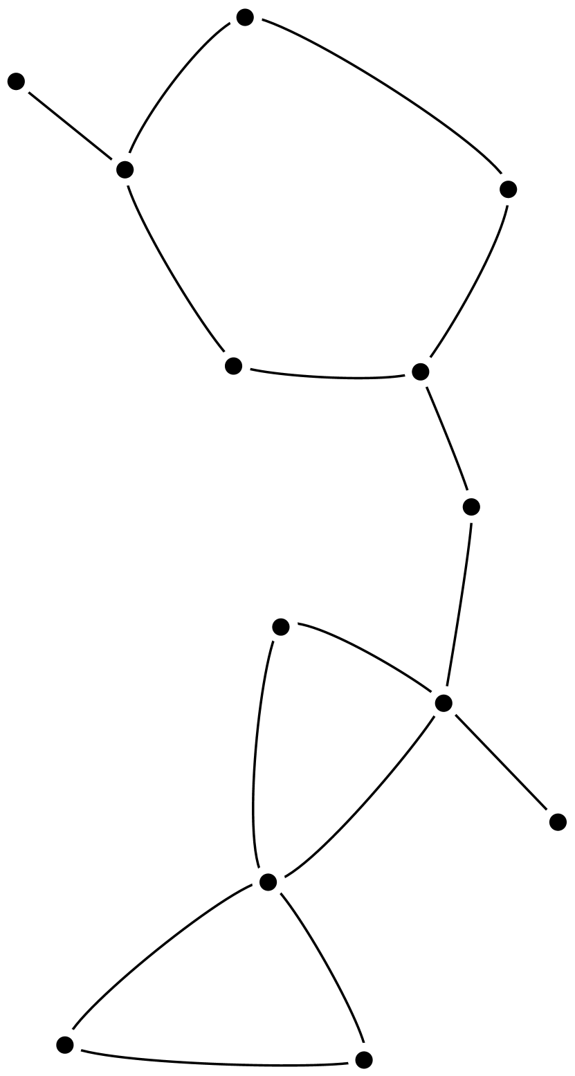
(a) the graph

(b) the black region

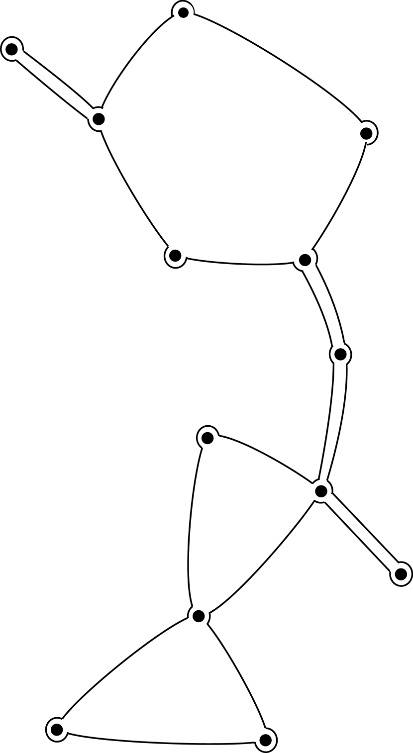
(c) the curve $\omega$

Figure 1. Desingularization of a graph

The next lemma describes an important class of essentially disconnecting boundary graphs:

Lemma 5.2.

Let $G$ be a boundary graph of saddle connections in $S$, obtained as $\omega$-limit set of a not self-intersecting geodesic, and such that every cycle of $G$ disconnects $S$. Then $G$ is essentially disconnecting.

Proof.  Let $U_{\sigma}$ be as in Lemma 5.1. Since, by assumption, every cycle in $G$ disconnects $S$, the complement $S\setminus\mathcal{C}$ of any cycle $\mathcal{C}$ in $G$ has exactly two connected components, only one disjoint from $U_{\sigma}$; let us color this component in black.

Furthermore, the fact that $G$ is a boundary graph implies that every edge of $G$ is contained in at most one cycle; as a consequence, $S\setminus G$ is formed by the part $P$ of $S$ containing $U_{\sigma}$ with $G$ as a boundary, and by the black connected components determined by the cycles in $G$.

Now we desingularize $G$ to a curve $\gamma$ in the following way, clearly equivalent to the construction above: near a pole connecting two (or more) cycles, we paint in black a little ball; and we replace each spike by a little black strip following its path. In this way we get a connected black region (see Figure 1).

Let $\gamma$ be the boundary of the black region we have constructed in this way. Clearly $\gamma$ is (homotopic to) a desingularization of $G$ and, because it separates a black region from a white one, by definition $\gamma$ disconnects $S$. It follows that $G$ is essentially disconnecting. $\Box$

So, we know that if every cycle is disconnecting then the graph is essentially disconnecting, while (generalizing Example 4.2 above) we can construct examples with an arbitrarily high number of disconnecting cycles (and at least one non disconnecting cycle) which are not essentially disconnecting.

We can now state the analogous of Equation (5.1) for case 4 of Theorem 4.3.

Theorem 5.1.

Let $S$ be a compact Riemann surface and $\nabla$ a meromorphic connection on $S$, with poles $p_{1},\dots,p_{r}\in S$. Let $S^{0}=S\setminus\{p_{1},\dots,p_{r}\}$. Let $\sigma\colon[0,\varepsilon_{0})\to S^{0}$ be a maximal geodesic for $\nabla$ having as $\omega$-limit set an essentially disconnecting boundary graph of saddle connections $G$. Let $P$ the part of $S$ having $G$ as boundary and containing the support of $\sigma$. Then

(5.2) $$\sum_{p_{i}\in P}\mathrm{Re}\,\mathrm{Res}_{p_{i}}(\nabla)=-1+2g_{\hat{P}}\;,$$

where $g_{\hat{P}}$ is the genus of the filling of $P$ (see Definition 5.2).

Proof.  Let $U$ be a connected open neighborhood of the support of $\sigma$ as in Lemma 5.1; without loss of generality we can assume that the support of $\sigma$ is completely contained in $U_{\sigma}$.

Consider a generic point $z_{0}\in G\cap S^{0}$. Using the local isometry $J$ near $z_{0}$ we see that we can find a geodesic $\tau\colon[0,\varepsilon)\to U_{\sigma}$ issuing from $z_{0}$ intersecting $\sigma$ transversally infinitely many times and making an angle $\alpha$ close to $\pi/2$ with the geodesic segment in $G$ passing through $z_{0}$.

Let $p_{0}\in U_{\sigma}$ be a point of intersection between $\sigma$ and $\tau$, and let $p_{1}\in U_{\sigma}$ be the next (following $\sigma$) point of intersection between $\sigma$ and $\tau$; necessarily $p_{1}\neq p_{0}$ because $\sigma$ has no self-intersections. The union of the segments of $\sigma$ and $\tau$ between $p_{0}$ and $p_{1}$ is a geodesic 2-cycle $\gamma$ contained in $U_{\sigma}$. The first observation is that the two external angles of $\gamma$ must have opposite signs. Indeed, if they had the same sign (roughly speaking, if $\sigma$ leaves and comes back to $\tau$ on the same side of $\tau$) then $\gamma$ would be the boundary of a part of $S$ contained in $U_{\sigma}$, and thus containing no poles, against Remark 3.2. The second observation is that $p_{1}$ must be closer (along $\tau$) to $G$ than $p_{0}$. Indeed, $\gamma$ disconnects $S$, because $G$ is essentially disconnecting; if $p_{1}$ were farther away from $G$ than $p_{0}$ then the support of $\sigma$ after $p_{1}$ would be contained in the connected component of $S\setminus\gamma$ disjoint from $G$, impossible (notice that after $p_{1}$ the geodesic $\sigma$ cannot intersect $\gamma$ anymore, because $\sigma$ has no self-intersections and any further intersection with the segment of $\tau$ contained between $p_{0}$ and $p_{1}$ would be on the same side of $\tau$ and thus can be ruled out as before).

Repeating this argument starting from $p_{1}$ we get a sequence $\{p_{n}=\sigma(t_{n})=\tau(s_{n})\}$ of points of intersections between $\sigma$ and $\tau$, with $t_{n}$ increasing, $s_{n}$ decreasing, and $p_{n}\to z_{0}$. Furthermore, if we denote by $\gamma_{n}$ the geodesic 2-cycle bounded by the segments of $\sigma$ and $\tau$ between $p_{n}$ and $p_{n+1}$, we also know that the external angles of $\gamma_{n}$ have opposite signs.

Since $G$ is essentially disconnecting, for $n$ large enough $\gamma_{n}$ disconnects $S$; let $P_{n}$ be the connected component of $S\setminus\gamma_{n}$ not containing $G$. Notice that the poles contained in $P_{n}$ are exactly the same contained in $P$, because $\gamma_{n}\subset U_{\sigma}\setminus G$. Furthermore, since the $\gamma_{n}$ are eventually homotopic to desingularizations of $G$, for $n$ large enough the genus of the filling of $P_{n}$ becomes equal to $g_{\hat{P}}$, the genus of the filling of $P$.

Up to a subsequence, we can assume that the directions of both $\sigma^{\prime}(t_{n})$ and $\sigma^{\prime}(t_{n+1})$ converge to a direction in $z_{0}$, necessarily the direction of the geodesic passing through $z_{0}$ contained in $G$. Since the external angles of $\gamma_{n}$ have opposite signs, it follows that their sum must converge to 0. But, by Corollary 3.2 and the arguments above, this sum must be eventually constant; so it must be 0, and (5.2) follows recalling again Corollary 3.2. $\Box$

In particular, [AT11, Theorem 4.6] is now a consequence of Theorems 4.3 and 5.1 (and Remark 4.4).

The formula (5.2) gives a necessary condition for the existence of geodesics on $S$ having as $\omega$-limit set an essentially disconnecting boundary graph of saddle connections. In particular, if no sum of real parts of residues is an odd integer number of the form $-1+2g$ then no such geodesic can exist on $S$.

The next statement contains a similar necessary condition for the existence of isolated vertices in a boundary graph of saddle connections:

Proposition 5.1.

Let $S$ be a compact Riemann surface and $\nabla$ a meromorphic connection on $S$. Let $p$ be a pole belonging to a boundary graph of saddle connections $G$ which is an $\omega$-limit set for a not self-intersecting geodesic $\sigma$. Suppose that $p$ is the vertex of only one arc $\rho$ of the graph. Then

$$\mathrm{Re}\,\mathrm{Res}_{p}(\nabla)=-\frac{1}{2}\;.$$

Proof.  Let $\tau$ be a geodesic crossing transversally $\rho$ at a point $q$ near $p$. The geodesic $\sigma$ must intersect both sides (with respect to $\rho$) of $\tau$ infinitely many times. Indeed, if it would intersect eventually only one side, arguing as in the previous proof we would see that the external angles at consecutive intersections would have opposite signs; and this would force the existence of points in $G$ close to $p$ but not belonging to $\rho$, impossible.

So we can construct a sequence $\{\sigma_{n}\}$ of segments of $\sigma$ connecting a point $p_{n}$ on one side of $\tau$ to a point $q_{n}$ on the other side of $\tau$, with both points of intersection converging to $q$. Let $\gamma_{n}$ be the geodesic 2-cycle consisting in $\sigma_{n}$ and the segment of $\tau$ between $p_{n}$ and $q_{n}$; eventually, $\gamma_{n}$ must be contained in a simply connected neighbourhood of $p$, and thus it is the boundary of a part $P_{n}$ of $S$ containing $p$ and no other poles. Notice that the genus of the filling of $P_{n}$ is zero.

An argument similar to the one used above shows that the external angles of $\gamma_{n}$ must have the same sign. Up to a subsequence, we can also assume that the direction of $\sigma$ both at $p_{n}$ and at $q_{n}$ converge to the same direction (which is the direction of $\rho$ at $q$); thus the sum of the external angles of $\gamma_{n}$ must tend to $\pi$. Applying Corollary 3.2 to $P_{n}$ we get (that this sum must be constant and) that

$$\pi=2\pi\bigl{(}1+\mathrm{Re}\,\mathrm{Res}_{p}(\nabla)\bigr{)}\;,$$

which gives the assertion. $\Box$

So, in particular, if all the poles have the real part of the residue different from $-1/2$, the graph cannot have vertices belonging to one arc only — and thus in particular it cannot have spikes.

Remark 5.2.  With the same argument as in Proposition 5.1 we see that if $p$ is a vertex belonging only to two arcs that are spikes, then the real part of its residue must be zero.

6. Non-compact Riemann surfaces

In this section we shall generalize some of the results of Section 4 to non-compact Riemann surfaces. We shall limit ourselves to consider Riemann surfaces $S$ that can be realized as an open subset of a compact Riemann surface $\hat{S}$. In this setting, all the results depending only on the local structure of geodesics still hold; for instance, Proposition 4.1, Lemmas 4.1 and 4.2, and Theorem 4.1 go through without any changes.

It is also easy to adapt Theorem 4.2. Indeed, the definition of singular line field on a compact Riemann surface $\hat{S}$ used in [Hou81] is that of regular line field defined on an open subset $S^{0}$ of $\hat{S}$, and the singular set is by definition $\hat{S}\setminus S^{0}$. In particular, if we consider the $\omega$-limit set $W$ of a geodesic $\sigma\colon I\to S^{0}$ in $\hat{S}$ (and not only in $S$) then $W\cap\partial S$ is automatically invariant with respect to any line field associated to $\sigma$. Therefore arguing as in the proof of Theorem 4.2 we get the following result.

Theorem 6.1.

Let $S$ be an open connected subset of a compact Riemann surface $\hat{S}$. Let $\nabla$ be a meromorphic connection on $S$, and denote by $S^{0}\subseteq S$ the complement in $S$ of the poles of $\nabla$. Let $\sigma\colon[0,\varepsilon_{0})\to S^{0}$ be a maximal not self-intersecting geodesic for $\nabla$. Then the possible minimal sets for $\sigma$ are the following:

1. a pole of $\nabla$;

2. a closed simple curve contained in $S^{0}$, which is a closed geodesic for $\nabla$, and in this case the $\omega$-limit set of $\sigma$ coincides with this closed geodesic;

3. a point in $\partial S\subset\hat{S}$;

4. all of $\hat{S}$, and in this case $\hat{S}$ is a torus.

Finally, in order to generalize Theorem 4.3 we need to consider saddle connections escaping to infinity, i.e., leaving any compact subset of $S$.

Definition 6.1  A diverging saddle connection for a meromorphic connection on a Riemann surface $S$ is a maximal geodesic $\sigma\colon(-\varepsilon_{-},\varepsilon_{+})\to S^{0}$ satisfying one of the allowing conditions:

• $\sigma(t)$ leaves every compact subset of $S$ for both $t\to-\varepsilon_{-}$ and $t\to\varepsilon_{+}$; or

• $\sigma(t)$ leaves every compact subset of $S$ for $t\to-\varepsilon_{-}$ and tends to a pole for $t\to\varepsilon_{+}$; or

• $\sigma(t)$ tends to a pole for $t\to-\varepsilon_{-}$ and leaves every compact for $t\to\varepsilon_{+}$.

A diverging graph of saddle connections is a connected planar graph in $S$ whose vertices are poles and whose arcs are disjoint saddle connections, with at least one of them diverging. A spike is a saddle connection of a graph which does not belong to any cycle of the graph.

A diverging boundary graph of saddle connections (or diverging boundary graph) is a diverging graph of saddle connections which is also the boundary of a connected open subset of $S$. A diverging boundary graph is disconnecting if its complement in $S$ is not connected.

Using these definitions, the following theorem generalizes Theorem 4.3 describing the possible $\omega$-limit sets of geodesics for a meromorphic connection on a non-compact Riemann surface of this kind.

Theorem 6.2.

Let $S$ be an open connected subset of a compact Riemann surface $\hat{S}$. Let $\nabla$ be a meromorphic connection on $S$, and denote by $S^{0}\subseteq S$ the complement in $S$ of the poles of $\nabla$. Let $\sigma\colon[0,\varepsilon_{0})\to S^{0}$ be a maximal geodesic for $\nabla$. Then one of the following possibilities occurs:

1. $\sigma(t)$ definitely leaves every compact subset of $S$ (i.e., it tends to the boundary of $S$ in $\hat{S}$); or

2. $\sigma(t)$ tends to a pole in $S$; or

3. $\sigma$ is closed; or

4. the $\omega$-limit set of $\sigma$ is the support of a closed geodesic; or

5. the $\omega$-limit set of $\sigma$ is a (possibly diverging) boundary graph of saddle connections; or

6. the $\omega$-limit set of $\sigma$ is all of $\bar{S}=S\cup\partial S$; or

7. the $\omega$-limit set of $\sigma$ has non-empty interior and non-empty boundary in $S$, and each component of its boundary is a (possibly diverging) graph of saddle connections with no spikes and at least one pole; or

8. $\sigma$ intersects itself infinitely many times.

Furthermore, in cases 3 or 4 the support of $\sigma$ is contained in only one of the components of the complement of the $\omega$-limit set, which is a part $P$ of $S$ having the $\omega$-limit set as boundary.

Proof.  Suppose that $\sigma$ is not closed (case 3) and does not self-intersect infinitely many times (case 8). Up to changing the starting point, we can suppose that $\sigma\colon[0,\varepsilon_{0})\to S^{0}$ does not self-intersect at all.

If $\sigma$ definitely leaves every compact set of $S$, we are in case 1 and we are done. Otherwise, the $\omega$-limit set $W$ of $\sigma$ must intersect $S$. We can then argue as in the proof of Theorem 4.3 using Theorems 4.1 and 6.1, and we are done. $\Box$

Remark 6.1  When the $\omega$-limit set is a non diverging graph it is possible to find conditions on the residues of the poles involved analogous to those described in Section 5, assuming it is disconnecting and the boundary of a relatively compact part.

7. Geodesics on the torus

In this section we study in detail the geodesics for holomorphic connections on the torus. We remark that, by Theorem 2.1, we cannot have holomorphic connections on Riemann surfaces different from the torus. Moreover, Proposition 4.2 tells us that this is the only case in which all the surface $S$ can be a minimal set (and a minimal set for an associated line field, and thus Theorem 2.2 implies that the connection must be holomorphic).

So, our goals are: to characterize holomorphic connections on a torus, and to study their geodesics.

We recall that a complex torus can be realized as a quotient of $\mathbb{C}$ under the action of a rank-2 lattice, generated over $\mathbb{R}$ by two elements $\lambda_{1}$, $\lambda_{2}\in\mathbb{C}$. Without loss of generality we can assume that one of the two generators is 1 and the other is a $\lambda\in\mathbb{C}$ with $\mathrm{Im}\,\lambda>0$. We shall denote by $T_{\lambda}$ the torus associated to $\lambda$.

The next elementary result characterizes holomorphic connections on a torus.

Lemma 7.1.

Every holomorphic connection on a torus is the projection of a holomorphic connection on the cover $\mathbb{C}$ represented by a constant global form $a\,dz$, for a suitable $a\in\mathbb{C}$.

Proof.  Let $\nabla$ be a holomorphic connection on a torus $T_{\lambda}$. Since the tangent bundle of a torus is trivial, we can find a global holomorphic $(1,0)$-form $\eta$ representing $\nabla$ by setting $\nabla e=\eta\otimes e$, where $e$ is a global nowhere vanishing section of the tangent bundle.

Let $\pi\colon\mathbb{C}\to T_{\lambda}$ be the universal covering map, and let $\tilde{\eta}=\pi^{*}\eta$; it is a holomorphic $(1,0)$-form on $\mathbb{C}$. Thus we can write $\tilde{\eta}=f\,dz$, for a suitable entire function $f$; we have to prove that $f$ is constant.

Let $\tau_{t}\colon\mathbb{C}\to\mathbb{C}$ be given by $\tau_{t}(z)=z+t$. Since $\pi\circ\tau_{1}=\pi\circ\tau_{\lambda}=\pi$, it follows that $\tau^{*}_{1}\tilde{\eta}=\tau^{*}_{\lambda}\tilde{\eta}=\tilde{\eta}$. But this is equivalent to $f(z+1)=f(z+\lambda)=f(z)$ for all $z\in\mathbb{C}$, and thus $f$ must be a bounded entire function, that is a constant. $\Box$

The next step consists in studying the geodesics for a holomorphic connection $\nabla$ on a torus. To do this, we shall study geodesics for the associated connection $\tilde{\nabla}$ on $\mathbb{C}$ represented by a constant form $a\,dz$ and then project them to the torus (all geodesics on the torus are obtained in this way: see [AT11, Proposition 3.1]).

Let $\tilde{\sigma}$ be a geodesic for $\tilde{\nabla}$ issuing from a point $z_{0}\in\mathbb{C}$ with tangent vector $v_{0}$. We first consider the trivial case $a=0$. In this case, the local isometry $J$ is given by $J(z)=cz$, with $c\in\mathbb{C}^{*}$. So, applying equation (2.4) in Proposition 2.2 we obtain

$$c\tilde{\sigma}(t)=cv_{0}t+cz_{0}\;,$$

which means that $\tilde{\sigma}(t)=v_{0}t+z_{0}$ and the geodesics are the euclidean ones. Thus in this trivial case the geodesics on $T_{\lambda}$ are exactly projections of straight lines.

If $a\neq 0$, the local isometry $J$ is given by $J(z)=\frac{1}{a}\exp(az)$. We apply again equation (2.4) in Proposition 2.2 to get

$$\frac{1}{a}\exp(a\tilde{\sigma}(t))=\exp(az_{0})v_{0}t+\frac{1}{a}\exp(az_{0})\;,$$

which we can solve to obtain

(7.1) $$\tilde{\sigma}(t)=z_{0}+\frac{1}{a}\log(1+av_{0}t)\;,$$

where $\log$ is the branch of the logarithm with $\log 1=0$ defined along the half-line $t\mapsto 1+av_{0}t$.

So in general the geodesics for $\tilde{\nabla}$ are not straight lines, unless $av_{0}\in\mathbb{R}$. However, every (projection of a) straight line in a torus is the support of a geodesic for a suitable (non-trivial) holomorphic connection:

Proposition 7.1.

Let $T_{\lambda}$ be a complex torus, and $\pi\colon\mathbb{C}\to T_{\lambda}$ the usual covering map. Let $\ell$ be a straight line in $\mathbb{C}$ issuing from $z_{0}\in\mathbb{C}$ and tangent to $v_{0}\in\mathbb{C}^{*}$. Then:

• $\pi(\ell)$ is the support of a geodesic $\sigma$ for the holomorphic connection $\nabla$ represented by the global form $\eta=a\,dz$ with $a\in\mathbb{C}^{*}$ if and only if $v_{0}\in\mathbb{R}\bar{a}$;

• $\pi(\ell)$ is the support of a closed geodesic $\sigma$ for the holomorphic connection $\nabla$ represented by the global form $\eta=a\,dz$ if and only if $v_{0}\in\mathbb{R}\bar{a}$ and $\bar{a}\in\mathbb{R}^{*}(\mathbb{Z}\oplus\mathbb{Z}\lambda)$.

Proof.  For any $a\in\mathbb{C}^{*}$, the unique geodesic $\sigma$ in $T_{\lambda}$ issuing from $\pi(z_{0})$ and tangent to $d\pi_{z_{0}}(v_{0})$ is $\sigma=\pi\circ\tilde{\sigma}$, where $\tilde{\sigma}$ is given by (7.1). Then the support of $\sigma$ coincides with $\pi(\ell)$ if and only if $\tilde{\sigma}$ is a parametrization of $\ell$, and this happens if and only if $av_{0}\in\mathbb{R}$, which is equivalent to $v_{0}\in\mathbb{R}\bar{a}$.

Assume now $v_{0}\in\mathbb{R}\bar{a}$. Then $\sigma$ is closed if and only if $\tilde{\sigma}(t_{0})=z_{0}+m+n\lambda$ for suitable $t_{0}\in\mathbb{R}^{*}$ and $m$, $n\in\mathbb{Z}$, that is if and only if

$$a(m+n\lambda)=\log(1+av_{0}t_{0})\;.$$

Recalling that $av_{0}\in\mathbb{R}$, this can happens if and only if $\bar{a}=r(m+n\lambda)$ for a suitable $r\in\mathbb{R}^{*}$, and we are done. $\Box$

Some of the geodesics given by Proposition 7.1 are closed, but none of them can be periodic. We prove this in the next proposition, where we characterize closed geodesics.

Proposition 7.2.

Let $\nabla$ be a holomorphic connection on the torus $T_{\lambda}$ represented by a global form $\eta=a\,dz$. Let $\sigma\colon[0,\infty)\to T_{\lambda}$ be a (non-constant) closed geodesic for $\nabla$. Then:

• if $a\neq 0$ then the support of $\sigma$ is the projection of a straight line parallel to $\bar{a}$ in the covering space $\mathbb{C}$, and $\sigma$ cannot be periodic;

• if $a=0$ then $\sigma$ is periodic.

Proof.  If $a=0$, the geodesics are the euclidean ones and so, once $\sigma$ is closed, it must also be periodic.

So let us study the problem when $a\neq 0$. In order for $\sigma$ to be closed and non-trivial, (7.1) implies that we must have

$$\frac{1}{a}\log(1+av_{0}\bar{t})=n+m\lambda$$

for suitable $\bar{t}\in\mathbb{R}^{*}$ and $n$, $m\in\mathbb{Z}$, not both zero, where $v_{0}=\tilde{\sigma}^{\prime}(0)\neq 0$ and $\tilde{\sigma}$ is the lifting of $\sigma$ given by (7.1). Furthermore, since $\sigma$ is closed then $\tilde{\sigma}^{\prime}(\bar{t})$ must be parallel to $\tilde{\sigma}^{\prime}(0)$. The derivative $\tilde{\sigma}^{\prime}$ is given by

(7.2) $$\tilde{\sigma}^{\prime}(t)=\frac{v_{0}}{1+av_{0}t}\;;$$

so $1+av_{0}\bar{t}=e^{a(n+m\lambda)}$ must be real. Since $\bar{t}$ is real too, it follows that $av_{0}$ must be real, and hence $\tilde{\sigma}$ is a parametrization of a straight line parallel to $\bar{a}$, as claimed.

Finally, $\sigma$ is periodic if and only if $v_{0}=\tilde{\sigma}^{\prime}(0)=\tilde{\sigma}^{\prime}(\bar{t})$; but by (7.2) this can happen only if $a=0$, contradiction. $\Box$

Remark 7.1.  If the support of a geodesic $\sigma$ of a holomorphic connection on a torus is the projection of a straight line, then $\sigma$ is either closed or everywhere dense. In particular, Proposition 7.1 provides examples of cases 2 and 5 in Theorem 4.3.

In the last theorem of this section we study the geodesics which are not the projection of a straight line, and give a complete description of the possible $\omega$-limit sets of geodesics for holomorphic connections on a torus.

Theorem 7.1.

Let $\nabla$ be a holomorphic connection on the complex torus $T_{\lambda}$, represented by the global 1-form $\eta=a\,dz$. Let $\sigma\colon[0,T)\to T_{\lambda}$ be a maximal (non constant) geodesic for $\nabla$.

• If $a\neq 0$ then the $\omega$-limit set of $\sigma$ is (the closure of) the projection on $T_{\lambda}$ of a straight line $l\colon\mathbb{R}\to\mathbb{C}$ of the form $l(t)=\bar{a}t+b$ for a suitable $b\in\mathbb{C}$. In particular:

  1. if $\bar{a}\in\mathbb{R}^{*}(\mathbb{Z}\oplus\lambda\mathbb{Z})\setminus\{0\}$ then either

     • $\sigma$ is closed, non periodic, and its support is the projection of the line $l$; or

     • $\sigma$ is not closed, but its $\omega$-limit set is a closed geodesic whose support is the projection of the line $l$;

  2. if $\bar{a}\notin\mathbb{R}^{*}(\mathbb{Z}\oplus\lambda\mathbb{Z})\setminus\{0\}$ then the $\omega$-limit set of $\sigma$ is all of $T_{\lambda}$.

• If $a=0$ then $\sigma$ is the projection of a line of the form $l(t)=v_{0}t+b$, where $v_{0}=\sigma^{\prime}(0)$. In particular:

  • if $v_{0}\in\mathbb{R}^{+}(\mathbb{Z}\oplus\lambda\mathbb{Z})$ then $\sigma$ is closed and periodic;

  • if $v_{0}\notin\mathbb{R}^{+}(\mathbb{Z}\oplus\lambda\mathbb{Z})$ then $\sigma$ is not closed and its $\omega$-limit set is all of $T_{\lambda}$.

Proof.  If $a=0$, we know that the geodesics are the projection of euclidean straight lines, and the statement follows. So let us assume $a\neq 0$.

Let $\tilde{\sigma}\colon[0,T)\to\mathbb{C}$ be the lifting of $\sigma$ to the covering space $\mathbb{C}$. By (7.1) the lifting $\tilde{\sigma}$ is given by

$$\tilde{\sigma}(t)=z_{0}+\frac{1}{a}\log(1+av_{0}t)=z_{0}+\frac{\bar{a}\log(1+av_{0}t)}{|a|^{2}}\;,$$

where $v_{0}=\tilde{\sigma}^{\prime}(0)$. When $t\to T$ it is easy to see that $\mathrm{Im}\,\log(1+av_{0}t)=\mathrm{Arg}(1+av_{0}t)$ converges to a finite limit, while $\mathrm{Re}\,\log(1+av_{0}t)=\log|1+av_{0}t|$ tends to $+\infty$ if $av_{0}\notin\mathbb{R}^{-}$, to $-\infty$ otherwise. It follows that $\tilde{\sigma}$ is asymptotic to a line of the form $l(t)=\bar{a}t+b$ for a suitable $b\in\mathbb{C}$, and thus the $\omega$-limit of $\sigma$ is the closure of the projection of this line in $T_{\lambda}$. The rest of the assertion follows from Propositions 7.1 and 7.2. $\Box$

References

- [Aba01] M. Abate. The residual index and the dynamics of holomorphic maps tangent to the identity. Duke Math. J., 107(1):173–207, 2001.
- [Aba10] M. Abate. Local discrete holomorphic dynamical systems. In Holomorphic dynamical systems. G. Gentili, J. Guenot, G. Patrizio eds., Lecture Notes in Math., Springer, Berlin, vol. 1998, pp. 1–55, 2010.
- [ABT04] M. Abate, F. Bracci and F. Tovena. Index theorems for holomorphic self-maps. The Annals of Math., 159(2):819–864, 2004.
- [ABT08] M. Abate, F. Bracci and F. Tovena. Index theorems for holomorphic maps and foliations. Indiana Univ. Math. J., 57: 2999–3048, 2008.
- [AT03] M. Abate and F. Tovena. Parabolic curves in . Abstr. Appl. Anal., 2003(5):275–294, 2003.
- [AT11] M. Abate and F. Tovena. Poincaré-Bendixson theorems for meromorphic connections and homogeneous vector fields. J. Differential Equations, 251:2612–2684, 2011.
- [AR14] M. Arizzi and J. Raissy. On Écalle-HakimÕs theorems in holomorphic dynamics. In Frontiers in complex dynamics. Eds. A. Bonifant, M. Lyubich, S. Sutherland. Princeton University Press, Princeton, 2014, pp. 387–449.
- [Cam78] C. Camacho. On the local structure of conformal mappings and holomorphic vector fields in . Astérisque, 59(60):83–94, 1978.
- [Cie12] K. Ciesielski. The Poincaré-Bendixson Theorem: from Poincaré to the XXIst century. Cent. Eur. J. Math., 10(6):2110–2128, 2012.
- [Éca81a] J. Écalle. Les fonctions résurgentes. Tome I: Les algèbres e fonctions rèsurgentes, volume 81-05. Publ. Math. Orsay, 1981.
- [Éca81b] J. Écalle. Les fonctions résurgentes. Tome II: Les fonctions résurgentes appliquées à l’itération, volume 81-06. Publ. Math. Orsay, 1981.
- [Éca85] J. Écalle. Les fonctions résurgentes. Tome III: L’équation du pont et la classification analytique des objects locaux, volume 85-05. Publ. Math. Orsay, 1985.
- [Hak97] M. Hakim. Transformations tangent to the identity. Stable pieces of manifolds. Université de Paris-Sud, Preprint, 145, 1997.
- [Hak98] M. Hakim. Analytic transformations of tangent to the identity. Duke mathematical journal, 92(2):403–428, 1998.
- [Hou81] J. Hounie. Minimal sets of families of vector fields on compact surfaces. J. Differential Geom., 16(4):739–744, 1981.
- [IY08] Y. Ilyashenko and S. Yakovenko. Lectures on analytic differential equations, volume 86. American Mathematical Society, Providence, RI, 2008.
- [Mil06] J. Milnor. Dynamics in one complex variable, 3rd ed. Princeton University Press, Princeton, 2006.
- [Mol09] L. Molino. The dynamics of maps tangent to the identity and with nonvanishing index. Trans. Amer. Math. Soc., 361(3):1597–1623, 2009.
- [Ron10] F. Rong. Absolutely isolated singularities of holomorphic maps of tangent to the identity. Pacific J. Math., 246(2):421–433, 2010.
- [Sch63] A. J. Schwartz. A generalization of a Poincaré-Bendixson theorem to closed two-dimensional manifolds. Amer. J. Math., 85(3):453–458, 1963.
- [Shc82] A.A. Shcherbakov. Topological classification of germs of conformal mappings with identical linear part. Moscow Univ. Math. Bull., 37:60–65, 1982.
- [ST88] R.A. Smith and E.S. Thomas. Transitive flows on two-dimensional manifolds. J. London Math. Soc. (2), 37:569–576, 1988.
- [Viv11] L. Vivas. Degenerate characteristic directions for maps tangent to the identity. Indiana Univ. Math. J., 61:2019-2040, 2012.