Echo spectroscopy of Anderson localization

Abstract

We propose a conceptually new framework to study the onset of Anderson localization in disordered systems. The idea is to expose waves propagating in a random scattering environment to a sequence of short dephasing pulses. The system responds through coherence peaks forming at specific echo times, each echo representing a particular process of quantum interference. We suggest a concrete realization for cold gases, where quantum interferences are observed in the momentum distribution of matter waves in a laser speckle potential, and discuss in detail corresponding echoes in momentum space for sequences of one and two dephasing pulses. Our proposal defines a challenging, but arguably realistic framework promising to yield unprecedented insight into the mechanisms of Anderson localization.

I Introduction

Coherent chaotic scattering is a defining feature of disordered quantum systems. Its manifestations range from coherence peaks in scattering cross sections over weak localization and quantum fluctuation phenomena in metals, to strong Anderson localization 50yearsAL . Phenomena of this type have been observed with light ALlight1 ; ALlight2 or microwaves ALmicrowaves , in electronic conductors AL , with cold atomic gases Chabe2008 ; Billy2008 ; Roati2008 ; Kondov2011 ; AL3DPalaiseau ; AL3DFlorence , photonic crystals ALpc1 ; ALpc2 , and classical waves ALothers . Semiclassically, quantum coherence is understood in terms of the interference of Feynman path amplitudes. Quantum effects arise when classically distinct amplitudes interfere to yield non-classical contributions to physical observables, see Fig. 1. For instance, coherent backscattering (CBS) and weak localization akkermans2006 are due to the interference of mutually time reversed paths. Similarly, coherent forward scattering is caused by the concatenation of two such processes, or again by the interference of two self retracing loops traversed in different order Karpiuk2012 ; Micklitz2014 ; Lee2014 , etc. Quantum coherent contributions are often discriminated from classical background contributions by their strong sensitivity to dephasing and decoherence. However, other than suppressing coherence, generic sources of decoherence – external magnetic fields, AC electromagnetic radiation, etc. – do not provide much insight into the mechanisms of quantum interference in disordered media. Furthermore, decoherence often acts as a source of heating (it certainly does so on the temperature scales relevant to cold atomic gases) and leads to an unwelcome nonequilibrium shake-up of the system.

In this paper, we suggest an alternative protocol for probing quantum coherence. Its advantage is that it offers much more specific information and at the same time is less intrusive than persistent external irradiation. The idea is to expose the quantum system to a source of dephasing only at specific ‘signal times’, $t_{1},t_{2},\dots$. The system then responds to this perturbation at ‘echo times’ $\tau_{1},\tau_{2},\dots$, which are in well-defined correspondence to the signal times. Each of these echoes corresponds to a specific mechanism of quantum-coherent scattering. For example, an echo at time $2t_{1}$ after a dephasing pulse applied at time $t_{1}$ is a tell-tale signature of the CBS effect (see Fig. 1 below). Likewise, an echo observed at time $2(t_{2}-t_{1})$ in response to two pulses at $t_{1}$ and $t_{2}>2t_{1}$ identifies a contribution to forward scattering coherence, etc. The observation of a temporal echo pattern thus realizes a highly resolved probe of quantum coherence in random scattering media.

The rest of the paper is organized as follows. In Section II we introduce the Feynman-path approach to coherence echoes and discuss real-space echo signals up to two-loop order. Section III discusses the first-order coherence echo in momentum space, while details about the second-order momentum-space signal are relegated to Appendix A. Section IV contains the systematic derivation of all results within a field-theoretical formalism. In the concluding Section V we suggest an experimental realization of echo spectroscopy with cold atoms. Further details on diffusion mode calculations are contained in Appendix B.

II Feynman path approach to coherence echoes

We consider a $d$-dimensional system of non-interacting quantum particles moving in a random potential and described by the Hamiltonian

$$\hat{H}={\hat{\mathbb{p}}^{2}\over 2m}+V(\hat{\mathbf{r}}).$$ (1)

The random potential $V$ is assumed to be an uncorrelated Gaussian process with covariance $\langle V(\mathbf{r})V(\mathbf{r}^{\prime})\rangle={1\over 2\pi\nu\tau}\delta(\mathbf{r}-\mathbf{r}^{\prime})$, where $\nu$ is the density of states per volume and $\tau$ the elastic scattering time. Central for our discussion is the retarded quantum correlation function

$$X\equiv\left\langle\hat{O}_{\mathbf{x}}(t)\hat{O}_{\mathbf{x}^{\prime}}(0)\right\rangle,$$ (2)

where the brackets stand for an average over quantum and disorder distributions, and $\hat{O}_{\mathbf{x}}=|\mathbf{x}\rangle\langle\mathbf{x}|$ is a projector onto a squeezed state defined by $\left\langle\mathbf{r}^{\prime}|\mathbf{x}\right\rangle=\frac{1}{(2\pi)^{d/4}}\frac{1}{(\Delta r)^{d/2}}\exp\left(-\frac{(\mathbf{r}^{\prime}-\mathbf{r})^{2}}{(2\Delta r)^{2}}+\frac{i}{\hbar}\mathbf{p}\cdot\mathbf{r}^{\prime}\right)$. The scale $\Delta r$ sets the spatial resolution of the operator, and $\mathbf{x}=(\mathbf{r},\mathbf{p})$ is a phase space vector comprising real space ($\mathbf{r}$) and momentum space ($\mathbf{p}$) coordinates. In the limit of infinitely sharp resolution $\hat{O}_{\mathbf{x}}\stackrel{{\scriptstyle\Delta r\to 0}}{{\longrightarrow}}|\mathbf{r}\rangle\langle\mathbf{r}|$ projects onto real-space coordinates, and the correlation function (2) may serve, e.g., as a building block for a point-contact transport observable. In the opposite limit $\hat{O}_{\mathbf{x}}\stackrel{{\scriptstyle\Delta r\to\infty}}{{\longrightarrow}}|\mathbf{p}\rangle\langle\mathbf{p}|$ projects onto momentum coordinates, and the correlation function relates to the cross section for the scattering process $\mathbf{p}\to\mathbf{p}^{\prime}$. Intermediate values of $\Delta r$ probe transitions between coherent-state-like wave packets of minimal quantum uncertainty centered around $\mathbf{x}$.

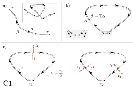
Figure 1: Physical observables represented in terms of pairs of retarded (solid lines) and advanced (dashed lines) Feynman path amplitudes. a) Copropagating Feynman paths, $\alpha=\beta$, yield the classical contribution to the two-point transition probability $\mathbf{r}\to\mathbf{r}^{\prime}$. Inset: weak localization loop. b) Coherent contribution, $\beta=\mathrm{T}\alpha$ to return probability $\mathbf{r}\to\mathbf{r}$, where $\mathrm{T}\alpha$ is the time reverse of $\alpha$. c) Coherent backscattering contribution in the presence of dephasing pulses (wiggly lines). While a pulse at time $t_{1}$ (dashed wiggly lines) suppresses the phase coherence of generic loops, it affects particle and hole amplitudes in synchronicity if the loop is traversed in time $\tau_{1}=2t_{2}$, where coherence is briefly restored. Right: synchronicity condition for a bi-temporal pulse at times $t_{1,2}$ is realized at traversal time $\tau_{2}=t_{1}+t_{2}$, where a coherence signal is observed.

To introduce the concept of coherence echoes, we consider in this section the case $\Delta r=0$ of a space-local two point correlation function. Within a Feynman path approach the expectation value (2) then assumes the form cmft

$$X=\sum_{\alpha,\beta}\,\left\langle e^{\frac{i}{\hbar}(S[\alpha]-S[\beta])}M_{\alpha\beta}\right\rangle,$$ (3)

where $\alpha,\beta$ are paths connecting $\mathbf{r}$ and $\mathbf{r}^{\prime}$ in time $t$, $S[\alpha]$ is the corresponding classical action, $M_{\alpha\beta}$ is a container symbol for matrix elements and semiclassical stability amplitudes, and brackets stand for an average over disorder configurations. The double sum is dominated by path configurations of nearly identical action $|S[\alpha]-S[\beta]|\lesssim\hbar$, all other contributions are effectively averaged out by large phase fluctuations. The set of contributing paths includes $\alpha=\beta$ [Fig. 1a)], which yields the classical, phase-insensitive approximation $X_{0}$ of the observable (3). Quantum corrections arise when paths branch out and subsequently recombine to form a phase coherent correction [Fig. 1a) inset]. One may think of the internal loop included in this process as a ‘self energy’ modifying the classical propagation in terms of a loop returning to its point of origin [Fig. 1b)]. It is these loop structures, with external ‘classical legs’ detached that are probed by our present approach: coherence signals tested by echoes arise when the two observation points $\mathbf{r}\to\mathbf{r}^{\prime}$ approach each other [Fig. 1b)]. The double sum is then given by an uninteresting classical contribution $\alpha=\beta$, and an equally strong quantum contribution $\beta=\mathrm{T}\alpha$, where $\mathrm{T}\alpha$ is the time reversed of the path $\beta$, and which is equivalent to the above self energy correction.

Consider now a single external radiation pulse applied to the system at time $t_{1}>0$ [Fig. 1c)]. At $t_{1}$ a particle propagating along $\alpha$ is at coordinate $\mathbf{r}(t_{1})$, while a particle propagating along $\mathrm{T}\alpha$ is at $\mathbf{\mathbf{r}}(t-t_{1})$, where $t$ is the loop traversal time selected by the moment of observation. In general, these coordinates differ from each other, which means that the external pulse affects the quantum phases carried by the two amplitudes in different ways—causing dephasing. However, if the traversal time is such that $t_{1}=t/2$, then $\mathbf{r}(t_{1})=\mathbf{r}(t-t_{1})$, and coherence is briefly regained. Another way of stating the same fact emphasizes the time reversal symmetry essential to the coherent backscattering signal: at time $t=2t_{1}$, time reversal $t\to 2t_{1}-t$ relative to the signal time $t_{1}$ is restored and the conditions for phase coherence apply. An observation of the system at time $t=2t_{1}\equiv\tau_{1}$ probes path pairs of just this ‘resonant’ length, which can be witnessed by the formation of a coherence peak in the observable $X$.

II.1 Perturbed quantum diffusion

To obtain a quantitative understanding of the echo signal, we consider a weakly disordered medium in which the paths entering individual segments of pair propagation (the double lines in Fig. 1) describe diffusion. For fixed initial and final coordinates $\mathbf{r}$ and $\mathbf{r}^{\prime}$ and propagation time $t$, the sum over all co-propagating paths is described by a classical diffusion propagator $\Pi_{\mathrm{D}}(\mathbf{r},\mathbf{r}^{\prime};t)$, or ‘diffuson’ for brevity akkermans2006 . The diffuson solves the diffusion equation $(\partial_{t}-D\partial^{2}_{\mathbf{r}})\Pi_{\mathrm{D}}(\mathbf{r},\mathbf{r}^{\prime};t)=\delta(\mathbf{r}-\mathbf{r}^{\prime})\delta(t)$, where $D=v^{2}\tau/d$ is the classical diffusion coefficient, $\tau$ the elastic scattering time, and $v=|\mathbb{p}|/m$ the velocity of particles of mass $m$. Likewise, the sum over all contributions to a segment $\mathbf{r}\to\mathbf{r}^{\prime}$ of counter-propagating paths is described by the propagator $\Pi_{\mathrm{C}}(\mathbf{r},\mathbf{r}^{\prime};t)$, the so-called Cooperon mode, which in the absence of dephasing obeys the same diffusion equation.

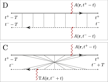
Figure 2: Coupling of diffuson (D) and Cooperon (C) to an external field $A=(\phi,\mathbf{a})$. The field acts at position $\mathbf{r}$ at the passage time of particle (solid upper line) and hole (dashed lower line), respectively. If these positions differ, dephasing occurs. In panel C, $\mathrm{T}A=\mathrm{T}(\phi,\mathbf{a})=(\phi,-\mathbf{a})$ indicates time reversal.

Let us now consider diffusive propagation in the presence of an external source of radiation, represented by a four-potential $A=(\phi,\mathbf{a})$, comprising a scalar and a vectorial component, $\phi=\phi(\mathbf{r},t)$ and $\mathbf{a}=\mathbf{a}(\mathbf{r},t)$, resp. To account for the externally imposed time dependence in a quantum diffusive process, we need to keep track of the traversal times of the participating Feynman paths. The situation is illustrated in Fig. 2, where ‘D’ is a diffuson mode comprising two amplitudes starting at times $t^{\pm}-T$, resp., and ending at $t^{\pm}$. We denote generally by $T$ the time required to traverse the segment, and the dashed lines are symbolic for the quantum scattering events causing diffusion. The wiggly lines represent the action of the external field at time $t^{\pm}-t$. If the two paths are traversed simultaneously, $t^{+}=t^{-}$, the potential affects the upper and lower line in the same way. In this case, the field does not destroy the mode, which is another way of saying that classical diffusion is not affected by quantum decoherence. In the Cooperon process, ‘C’, scattering paths are traversed in opposite order, as indicated by the ‘maximally crossed’ representation of scattering vertices. (Equivalently, one may flip the lower line, which leads to the un-crossed representation with co-oriented arrows employed in the rest of the figures). The sign change in the time reversed potential $\mathrm{T}A=\mathrm{T}(\phi,\mathbf{a})=(\phi,-\mathbf{a})$ reflects the time reversal symmetry breaking nature of external vector potentials. Likewise, a time-dependent scalar potential $\phi(t)$ will cause dephasing, unless an echo condition is met.

The influence of the field on the diffusion modes can be quantitatively described by diagrammatic perturbation theory EfrosPollack . Under the assumption that the external field alters quantum phases but is sufficiently weak not to change the classical trajectories themselves, the perturbed diffuson and Cooperon modes (${\rm M}={\rm D,C}$) are still governed by generalized diffusion equations

$$\mathcal{D}_{\mathrm{M}}\Pi_{\mathrm{M}}(\mathbf{r},\mathbf{r}^{\prime};t^{+},t^{-},T)=\delta(T)\delta(\mathbf{r}-\mathbf{r}^{\prime}),$$ (4)

$$\quad\mathcal{D}_{\mathrm{D}/C}=\partial_{t^{+}}\pm\partial_{t^{-}}-i[\phi(\mathbf{r},t^{+})-\phi(\mathbf{r},t^{-})]$$

$$\hskip 56.9055pt-D\left(\partial_{\mathbf{r}}+i[\mathbf{a}(\mathbf{r},t^{+})\mp\mathbf{a}(\mathbf{r},t^{-})]\right)^{2},$$ (5)

in which the field $A=(\phi,\mathbf{a})$ enters through a covariant derivative. For a given $A$, these ‘imaginary-time Schrödinger equations’ can be solved, e.g., by path-integral techniques EfrosPollack ; Feynman (see Appendix B). We here consider a situation without magnetic field, $\mathbf{a}=0$, and a scalar potential

$$\hbar\phi(\mathbf{r},t)=-\mathbf{r}\cdot\Delta\mathbf{p}f(t).$$ (6)

In the remainder of this section, we take $f(t)=\sum_{i=1}^{N}\delta(t-t_{i})$ to represent a sequence of short pulses, each of which applies a homogeneous force that transfers a momentum ${\Delta\mathbf{p}}$; the above weak field assumption requires that each transfered momentum be much smaller than the particle momentum, $|{\Delta\mathbf{p}}|\ll p$. The dephasing pulses realize the ideal form of effective $\delta$-kicks if they are shorter than the mean free time $\tau$. Longer pulses are also admissible and provide full echo contrast as long as they are symmetric around $t_{i}$.

II.2 First-order echo signal

The first-order quantum coherence contribution to the observable (2) involves two counter-propagating paths running synchronously between time $0$ and $t$, and thus has the time arguments $t^{+}=t,t^{-}=0,T=t$. For times $t<t_{1}$ before the first pulse, the single Cooperon contribution $X_{\rm C1}(t)=c/(Dt)^{d/2}$ is just the classical probability of return within time $t$, where $c$ is a numerical constant. Around the time $t=2t_{1}$, the signal is found to behave like

$$\delta X_{\text{C1}}(t) =X_{\rm C1}(t)e^{-|t-2t_{1}|/\tau_{\mathrm{e}}}.$$ (7)

This describes a near instantaneous destruction of the coherence contribution by the pulse at $t_{1}$ followed by a revival at the echo time $\tau_{1}=2t_{1}$ over a width

$$\tau_{\mathrm{e}}=\hbar^{2}/D\Delta p^{2}.$$ (8)

The complete derivation of this signal, allowing also for a generalization to more general pulse profiles, follows from the momentum-space results as described in Sec. III below. But the echo profile (7) can be readily understood by noting that the phases of the two amplitudes are affected as

$$\left\langle e^{i[\phi(\mathbf{r}(t_{1}))-\phi(\mathbf{r}(t-t_{1}))]}\right\rangle\simeq e^{-\frac{1}{2}\left\langle[\phi(\mathbf{r}(t_{1}))-\phi(\mathbf{r}(t-t_{1}))]^{2}\right\rangle},$$ (9)

where the angular brackets represent averaging over path configurations. Substituting the potential (6) and noting that for a diffusive process $\left\langle[\mathbf{r}(t)-\mathbf{r}(s)]^{2}\right\rangle\sim D|t-s|$ one then obtains (7). Also, one sees that the characteristic echo time (8) is determined by the time scale over which the phase mismatch between the two amplitudes reaches unity, $\left\langle(\Delta p\Delta x)^{2}\right\rangle\sim\Delta p^{2}D\tau_{\mathrm{e}}=\hbar^{2}$.

The first-order coherence signal (7) is suppressed directly after the C1 echo at time $\tau_{1}$. If, now, a second pulse is applied at time $t_{2}>\tau_{1}$, the coherence condition is met once more at $\tau_{2}\equiv t_{1}+t_{2}$, and another C1 echo will be observed [Fig. 1 c) second diagram]. In addition to this signal, however, such a bi-temporal pulse gives rise to further echoes, which probe more complex manifestations of quantum interference, to be discussed next.

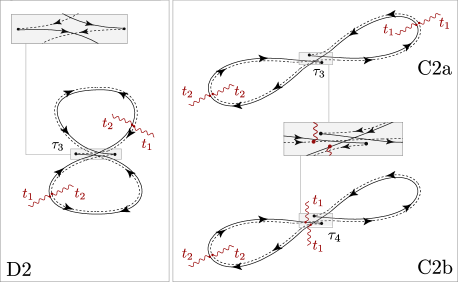
Figure 3: Higher-order coherence contributions to the return amplitude probed by bi-temporal pulsing. The dephasing vertices shown in the inset of the right panel are only present in the C2b process. For the definition of the observation times $\tau_{3,4}$ and further discussion, see text.

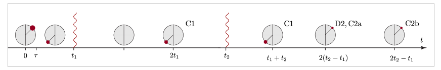
Figure 4: Chronology of quantum coherence echoes in the $k_{x}{-}k_{y}$ plane of momentum space. Echoes are indicated by red dots whose width/position hint at the signal strength/angular orientation on the elastic scattering manifold. From left to right: An initial state with well defined momentum yields the single-Cooperon (C1) backscattering peak after the transport time $\tau$. A first dephasing pulse at $t_{1}$ supresses the C1 signal, which reappears at the first echo time $\tau_{1}=2t_{1}$. A second pulse at $t_{2}$ generates the bi-pulse C1 echo at $\tau_{2}=t_{1}+t_{2}$. Two-mode echoes appear in the forward scattering direction at $\tau_{3}=2(t_{2}-t_{1})$ (D2, C2a) and $\tau_{4}=2t_{2}-t_{1}$ (C2b).

II.3 Probing higher-order quantum interference

We find that a double pulse selectively generates echo signals from two-loop contributions, as depicted in Fig. 3. Consider, for example, the D2 coherence process that describes the interference of paths along two loops which are traversed in the same direction (no time reversal required!), but in different order. During its traversal of the first loop, the particle is hit by the first pulse at time $t_{1}$. The particle then moves on into the second loop, where it is hit by the second pulse at time $t_{2}$. A straightforward assignment of travel times to path segments shows that the hole amplitude (going through the loops in opposite order) will experience the pulses in synchronicity, i.e. at the same spatial path coordinates, provided the time of traversal for each loop be $t_{2}-t_{1}$. In this case, the process becomes coherent, and an echo will be observed at $\tau_{3}\equiv 2(t_{2}-t_{1})$.

A similar argument shows that at the same time $\tau_{3}$ the Cooperon process C2a shown in Fig. 3—consisting of two counter-propagating loops traversed in the same order—becomes phase coherent, too. For that path configuration the coherence condition is satisfied at one more time $\tau_{4}\equiv 2t_{2}-t_{1}$ and this leads to one more echo C2b, also indicated in Fig. 3. Quantitative calculations below result in the two-loop echo contributions

$$\delta X_{\rm M}(t)=X_{\rm M}(t)e^{-|t-\tau_{\mathrm{M}}|/\tau_{\mathrm{e}}},\quad\mathrm{M=D2,C2a,C2b},$$ (10)

where $\tau_{\rm D2,C2a}=\tau_{3}$, $\tau_{\rm C2b}=\tau_{4}$, and $X_{\rm M}(t)$ are smoothly varying functions, whose detailed features follow from the results of the Appendix A. Here we note that the overall signal strength $X_{\rm M}$ is by a factor $(E\tau/\hbar)^{1-d}\ll 1$ smaller than the strength function $X_{\rm C1}$ of the C1 process and in this smallness reflects the relatively smaller phase volume available to the returning of higher-order path topologies.

Summarizing the discussion so far, Fig. 4 shows a typical chronology of echo signals in response to two applied pulses as a sequence of dots of varying strength and angular orientation. The latter refers to directional information encoded in momentum space, to be discussed next.

III Momentum space echoes

Although the essential classification of the system response in terms of echo times $\{\tau_{i}\}$ and corresponding path structures is universal, additional information can be obtained if observables different from the coordinate projectors $\hat{O}=|\mathbf{r}\rangle\langle\mathbf{r}|$ are chosen. Specifically, in this section we turn to the complementary limit of momentum projectors, $\hat{O}=|\mathbf{k}\rangle\langle\mathbf{k}|$, and look for echo signals in the scattering probability from $\mathbf{k}$ to $\mathbf{k}^{\prime}$. Since now initial and final momentum are fixed, the formal loop order is decreased by one compared to the real-space setting. Namely, an $n$-mode contribution to the momentum-space signal will be made of $(n-1)$ momentum integrals, and the corresponding $n$-loop signal in real space is recovered by one supplementary momentum integration. Also, quantum coherence in momentum space no longer constrains the initial and final positions, but instead requires an alignment of initial and final momenta, $\mathbf{k}^{\prime}=\pm\mathbf{k}$. Therefore, in a momentum resolved scattering experiment, the $\mathrm{C1}$ echo is observed as a contribution to the backscattering probability at $\mathbf{k}^{\prime}=-\mathbf{k}$. In contrast, two-mode contributions will peak in the forward direction $\mathbf{k}=\mathbf{k}^{\prime}$. Forward-scattering coherence has been recently identified as particularly interesting in connection with the onset of strong localization Karpiuk2012 ; Micklitz2014 ; Lee2014 .

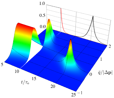
Figure 5: Single-mode Cooperon echo contrast $\delta X_{\text{C1}}(t,\bar{\mathbf{q}})/X_{0}$, given by (12), as function of time $t$ and momentum $\bar{q}$ [in units of $\tau_{\text{e}}$ and $\Delta p$ and for $\bar{\mathbf{q}}\parallel{\Delta\mathbf{p}}$], with a dephasing pulse at $t_{1}=10\tau_{\text{e}}$. The momentum kick ${\Delta\mathbf{p}}$ initially displaces the entire momentum distribution, then dephasing sets in, and the signal only revives at the echo time $\tau_{1}=2t_{1}$. The echo contrast at exact backsattering $\bar{q}=0$ is shown as the black curve in the side panel. The real-space signal (7) follows after integration over $\bar{\mathbf{q}}$.

In fact, coherence echoes in momentum space show a somewhat richer structure beyond the general forward and backward orientation. It is instructive to look first at the single-Cooperon coherent backscattering echo. Postponing a systematic derivation to the next Section IV, we state here merely the expected result Cherroret2012 :

$$\delta X_{\text{C1}}(t,\bar{\mathbf{q}}) =X_{0}\Pi_{\text{C}}(\bar{\mathbf{q}},t,0,t),$$ (11)

where $X_{0}={4\pi\over\nu}\tilde{\delta}(\epsilon_{\mathbb{k}}-\epsilon_{\mathbb{k}^{\prime}})$ with $\tilde{\delta}(\epsilon)=\frac{\hbar}{2\pi\tau}\frac{1}{\epsilon^{2}+(\hbar/2\tau)^{2}}$ is a broadened $\delta$-function keeping the arguments of the correlation function on-shell, and $\Pi_{\text{C}}(\bar{\mathbf{q}},t,0,t)$ is the Cooperon solution of the generalized diffusion equation (4) at momentum $\bar{\mathbf{q}}=\mathbf{k}+\mathbf{k}^{\prime}$ away from the backscattering direction.

In the absence of external potentials, the simple diffusion equation is solved by the Gaussian $\delta X_{\text{C1}}(t,\bar{\mathbf{q}})=X_{0}e^{-Dt\bar{\mathbf{q}}^{2}/\hbar^{2}}$, as recently predicted for a cold atom set up Cherroret2012 and consequently observed CBSexperiment . Now, in presence of the dephasing (6), the Cooperon takes the form

$$\delta X_{\text{C1}}(t,\bar{\mathbf{q}}) =X_{0}e^{-{D\over\hbar^{2}}\left(t\bar{\mathbf{q}}^{2}-2\bar{\chi}_{1}(t)\bar{\mathbf{q}}\cdot{\Delta\mathbf{p}}+\bar{\chi}_{2}(t){\Delta\mathbf{p}}^{2}\right)}.$$ (12)

A derivation of this result, including expressions of the auxiliary functions $\bar{\chi}_{1/2}$ for general pulse profiles $f(t)$ (eqs. (81) and (82)) can be found in Appendix B below. For a single $\delta$-pulse at time $t=t_{1}$, these functions simply vanish before the pulse and are $\bar{\chi}_{1}(t)=(2t_{1}-t)$ and $\bar{\chi}_{2}(t)=|2t_{1}-t|$ at times $t>t_{1}$ after the pulse. In that case, the echo contrast in the exact backward direction $\bar{\mathbf{q}}=0$ reads

$$\delta X_{\text{C1}}(t,0)=X_{0}e^{-\theta(t-t_{1})|t-2t_{1}|/\tau_{\text{e}}},$$ (13)

and thus describes a sharp drop at the pulse time $t_{1}$ followed by an exponential revival at the echo time $\tau_{1}=2t_{1}$. The corresponding real-space echo (7) follows upon integration of eq. (12) over $\bar{\mathbf{q}}$.

On the scale of ${\Delta\mathbf{p}}$, the momentum-space signal shows a rather interesting dynamics, as plotted in Fig. 5. Initially, the dephasing kick displaces the entire momentum distribution by ${\Delta\mathbf{p}}$, and thus also displaces the backscattering peak, which subsequently takes a finite time $\tau_{\text{e}}$ to dephase. As time increases, the point of highest contrast is found at $\bar{\mathbf{q}}_{0}(t)=\bar{\chi}_{1}(t){\Delta\mathbf{p}}/t$. It thus moves from $\bar{\mathbf{q}}_{0}(t_{1})={\Delta\mathbf{p}}$ towards the original position $\bar{\mathbf{q}}_{0}(2t_{1})=0$, reached at the echo time, and then continues onward to $\bar{\mathbf{q}}_{0}\to-{\Delta\mathbf{p}}$ at long times. The peak is severely suppressed at generic times, but revives with perfect contrast at $t=2t_{1}$ where $\bar{\chi}_{1}=0=\bar{\chi}_{2}$.

For pulses of finite resolution in time, but still symmetric around $t_{1}$, the peak always reaches the original position $\bar{\mathbf{q}}_{0}=0$ at $2t_{1}$ where the contrast penalty vanishes, implying a perfect revival, as a consequence of the general expressions (81) and (82). Only for an asymmetric pulse the contrast penalty generically remains finite, and the echo will appear with reduced contrast.

In contrast to the C1 echo discussed so far, the higher-order processes D2 and C2 show echoes in response to bi-temporal pulsing in the forward scattering direction. A detailed discussion of the intricacies of momentum-resolved two-mode echoes can be found in Appendix A. We first complete the general development of the theory by a systematic derivation of echo contributions via a field-theoretical approach.

IV Field theory

In this section we derive the results discussed so far within the framework of the diffusive nonlinear $\sigma$-model efetov . Compared to a direct perturbative ‘diagrammatic’ calculation, the $\sigma$-model greatly simplifies the handling of the vertex regions distinguishing individual echo contributions. It also ‘automatizes’ the identification of echo time structures, which in a diagrammatic framework have to be anticipated from the beginning. We use a simplified Keldysh version of the model AndreevKamenev ; LevchenkoKamenev ; AltlandKamenev , which is tailored to treat time dependent phenomena, and proceed to show how the theory yields the discussed echo structures. We invite readers not interested in technical details to skip this section and to proceed to “Summary and experimental realization”.

IV.1 Effective theory

Central to our discussion is a functional-integral partition function

$$\mathcal{Z}=\int DQ\,\exp(iS[Q]),$$ (14)

with effective action

$$iS[Q] ={\pi\nu\hbar\over 8}\int d\mathbf{r}\,{\rm tr}\left(2\partial^{\phi}Q(\mathbf{r})-D(\partial^{\mathbb{a}}Q(\mathbf{r}))^{2}\right),$$ (15)

describing quantum diffusion on time scales, $t\gg\tau$, and eventually Anderson localization on asymptotically large scales. Here, $\nu$ is the density of states per volume, $\tau$ the elastic scattering time, and $Q=\{Q^{\alpha\alpha^{\prime}}_{ss^{\prime},tt^{\prime}}\}$ is a unitary matrix field, $Q^{-1}=Q^{\dagger}$, bi-local in time $t,t^{\prime}$ and two-dimensional in two auxiliary spaces of Keldysh ($\mathrm{K}$) and time reversal ($\mathrm{T}$) variables, respectively. The $\mathrm{K}$-space indices $\alpha=\pm$ discriminate between retarded $(+)$ and advanced $(-)$ propagators. The $\mathrm{T}$-space indices $s=\pm$ track time reversal operations. For example, the matrix block $Q^{+-}_{+-}$ describes an interfering pair of retarded and advanced amplitudes which are counter-propagating in time, $Q^{+-}_{++}$ describes interference of co-propagating amplitudes, etc. The trace ‘tr’ in (15) includes summation over all indices, including continuous time, $\mathrm{tr}(A)=\sum_{\alpha,s}\int dt\,A^{\alpha\alpha}_{ss,tt}$. Likewise, matrix multiplication is defined as $(AB)^{\alpha\alpha^{\prime}}_{ss^{\prime},tt^{\prime}}=\int dt^{\prime\prime}\sum_{\alpha^{\prime\prime},s^{\prime\prime}}A^{\alpha\alpha^{\prime\prime}}_{ss^{\prime\prime},tt^{\prime\prime}}B^{\alpha^{\prime\prime}\alpha^{\prime}}_{s^{\prime\prime}s^{\prime},t^{\prime\prime}t^{\prime}}$. With these conventions, the matrix field $Q$ is defined to obey the nonlinear constraint

$$(Q^{2}(\mathbf{r}))_{tt^{\prime}}=\openone\delta(t-t^{\prime}),$$

where $\openone$ is the unit-matrix in $\mathrm{K}\otimes\mathrm{T}$. Invariance under time-reversal reflects in a second constraint

$$(Q_{tt^{\prime}})^{\mathrm{t}}=\sigma_{2}^{\mathrm{T}}Q_{-t^{\prime},-t}\sigma_{2}^{\mathrm{T}},$$ (16)

where $\mathrm{t}$ is transposition in $\mathrm{K}\otimes\mathrm{T}$ and the Pauli matrices $\sigma_{i}^{\mathrm{X}}$ act in $\mathrm{X}=\mathrm{K},\mathrm{T}$-space, respectively.

The particle matrix field $Q$ couples in Eq. (15) to the external fields via the covariant derivatives

$$\partial^{\phi}Q(\mathbf{r})_{ss^{\prime},tt^{\prime}} =[\partial_{t}-\partial_{t^{\prime}}+i\phi(\mathbf{r},st)+i\phi(\mathbf{r},s^{\prime}t^{\prime})]Q_{ss^{\prime},tt^{\prime}}(\mathbf{r}),$$ (17)

$$\partial^{\mathbb{a}}Q(\mathbf{r})_{ss^{\prime},tt^{\prime}} =[\partial_{\mathbf{r}}+is\mathbb{a}(\mathbf{r},st)-is^{\prime}\mathbb{a}(\mathbf{r},s^{\prime}t^{\prime})]Q_{ss^{\prime},tt^{\prime}}(\mathbf{r}).$$ (18)

The covariant form of these derivatives reflects the local U(1) gauge invariance of the theory. The sign structure in $\mathrm{T}$-space ensures that the covariant derivatives of the $Q$-field are consistent with the time reversal condition (16).

The action (15) is manifestly invariant under ‘rotations’ $Q_{0}=\sigma_{3}^{\mathrm{K}}\mapsto T_{0}\sigma_{3}^{\mathrm{K}}T_{0}^{-1}$, where $T_{0}=\mathrm{const.}$ is a matrix in $\mathrm{K}$-space and $Q_{0}=\sigma_{3}^{\mathrm{K}}$ a saddle point not containing interference terms, $(\sigma_{3}^{\mathrm{K}})^{+-}=(\sigma_{3}^{\mathrm{K}})^{-+}=0$. This saddle point describes the system before the appearance of diffusion modes, the sign structure in $\mathrm{K}$-space being a consequence of Green function causality. AndreevKamenev ; LevchenkoKamenev ; AltlandKamenev Transformations with $T_{tt^{\prime}}(\mathbf{r})$ slowly varying in space and time generates soft ‘Goldstone modes’ that represent physical diffusion modes, much like small $(\mathbf{r},t)$-dependent -rotations of the spins in a ferromagnet describe magnon modes. We therefore parametrize the relevant nonlinear field manifold by

$$Q(\mathbf{r}) =T(\mathbf{r})\sigma_{3}^{\mathrm{K}}T^{-1}(\mathbf{r})$$ (19)

and with smooth fluctuations $T$.

IV.2 Cooperon and diffuson modes

To explore the effect of soft mode fluctuations, we parameterize the rotation matrices as $T=e^{W/2}$ where the generators $W$ are chosen to anti-commute with the saddle point, $\big{[}\sigma_{3}^{\mathrm{K}},W\big{]}_{+}=0$. These generators are block off-diagonal in $\mathrm{K}$-space,

$$W=\left(\begin{matrix}&B\cr-B^{\dagger}&\end{matrix}\right)_{\mathrm{K}},\qquad B=\{B^{ss^{\prime}}_{tt^{\prime}}\},$$ (20)

their anti-hermitean structure required by the unitarity of $Q$. The time reversal symmetry relation (16) implies $(W_{tt^{\prime}})^{\mathrm{t}}=-\sigma_{2}^{\mathrm{T}}W_{-t^{\prime},-t}\sigma_{2}^{\mathrm{T}}$. For the $B$-matrices this means

$$B^{--}_{tt^{\prime}}=\bar{B}^{++}_{-t^{\prime},-t},\qquad B^{-+}_{tt^{\prime}}=-\bar{B}^{+-}_{-t^{\prime},-t},$$ (21)

where the overbar is complex conjugation. We will identify modes $B^{\pm\pm}$ of identical ($B^{\pm\mp}$ of opposite) time orientation of amplitudes as diffuson (Cooperon) modes, and define $B^{++}_{tt^{\prime}}\equiv D_{tt^{\prime}}$ and $B^{-+}_{tt^{\prime}}\equiv C_{tt^{\prime}}$ or in $\mathrm{T}$-space

$$B_{tt^{\prime}}=\left(\begin{matrix}D_{tt^{\prime}}&-\bar{C}_{-t^{\prime}-t}\crcr C_{tt^{\prime}}&\bar{D}_{-t^{\prime}-t}\end{matrix}\right).$$ (22)

The strategy now is to substitute the expansion

$$Q =T\sigma_{3}^{\mathrm{K}}T^{-1}\simeq\sigma_{3}^{\mathrm{K}}\left(1-W+W^{2}/2+\dots\right)$$ (23)

into the action (15) and to expand in $W$. There is no zeroth-order contribution, and the first order vanishes around the saddle point. To second order, the action decouples into two quadratic actions for diffuson and Cooperon, respectively,

$$iS^{(2)}_{\text{D}} =-\frac{\pi\nu\hbar}{2}\int dt\int dt^{\prime}\int d\mathbf{r}\,D_{t^{\prime}t}(\mathbf{r})\left(\partial_{t}+\partial_{t^{\prime}}+i\left[\phi(\mathbf{r},t)-\phi(\mathbf{r},t^{\prime})\right]-D\left(\partial_{\mathbf{r}}+i\left[\mathbb{a}(\mathbf{r},t)-\mathbb{a}(\mathbf{r},t^{\prime})\right]\right)^{2}\right)\bar{D}_{tt^{\prime}}(\mathbf{r}),$$ (24)

$$iS^{(2)}_{\text{C}} =-\frac{\pi\nu\hbar}{2}\int dt\int dt^{\prime}\int d\mathbf{r}\,C_{-t^{\prime}t}(\mathbf{r})\left(\partial_{t}-\partial_{t^{\prime}}+i\left[\phi(\mathbf{r},t)-\phi(\mathbf{r},t^{\prime})\right]-D\left(\partial_{\mathbf{r}}+i\left[\mathbb{a}(\mathbf{r},t)+\mathbb{a}(\mathbf{r},t^{\prime})\right]\right)^{2}\right)\bar{C}_{t,-t^{\prime}}(\mathbf{r}).$$ (25)

The kernels are just the differential operators (4). The correspondence with the diffusion modes $\Pi_{\text{D/C}}$ can be made more explicit by calculating the expectation values $\left\langle\dots\right\rangle^{(2)}\equiv\int D(D,C)\exp[iS^{(2)}_{\text{C}}+iS^{(2)}_{\text{C}}](\dots)$ with the quadratic action, where $D(D,C)$ stands for integration over the matrix-fields $D,C$. Since a complex Gaussian integral yields the inverse of the action kernel, the expectation values

$$\langle\bar{D}_{t^{+},t^{-}}(\mathbf{r})D_{t^{-}-T,t^{+}-T^{\prime}}(\mathbf{r}^{\prime})\rangle^{(2)} ={2\over\pi\nu\hbar}\Pi_{\text{D}}(\mathbf{r},\mathbf{r}^{\prime};t^{+},t^{-},T)\delta(T-T^{\prime}),$$

$$\langle\bar{C}_{t^{+},-t^{-}}(\mathbf{r})C_{-t^{-}-T,t^{+}-T^{\prime}}(\mathbf{r}^{\prime})\rangle^{(2)} ={2\over\pi\nu\hbar}\Pi_{\text{C}}(\mathbf{r},\mathbf{r}^{\prime};t^{+},t^{-},T)\delta(T-T^{\prime}),$$ (26)

obey Eqs. (4) and thus are identical to the modes considered there. For later reference, we note that the $\delta(T-T^{\prime})$-functions above are regularized to the shortest time scales $\sim\tau$ resolved by the field theory; they are to be understood as broadened Lorentzians with finite peak height $\delta(0)=\tau^{-1}$. (For completeness, we note that the Gaussian integrals are unit normalized, $\left\langle 1\right\rangle=1$, i.e. they do not yield a non-trivial ‘functional determinant’. The physical principle behind this is Green function causality, which implies the unit-valuedness of the determinants of the Cooperon and diffuson differential operators. For further discussion of this point, we refer to Refs. [AltlandKamenev, ; LevchenkoKamenev, ].)

IV.3 Generation of observables

Starting from this section, we focus on momentum-space coherences. As already discussed in Sec. III, momentum-resolved correlations provide additional information about the parity of interference processes under time-reversal, which complements the information contained in spatial correlations. A generalization of the formalism to the generic coherent states introduced in section II is straightforward. The relevant correlation function (2) then is

$$X(t,\mathbb{k},\mathbb{k}^{\prime})=\left\langle\left|\langle{\mathbf{k}^{\prime}}|\exp\{-iHt\}|\mathbf{k}\rangle\right|^{2}\right\rangle,$$ (27)

namely the ensemble-averaged scattering probability from $\mathbf{k}$ to $\mathbf{k}^{\prime}$ in time t. In order to compute this correlation function from the field theory, we introduce two source parameters $\alpha=\{\alpha^{\text{i}},\alpha^{\text{f}}\}$ together with the projectors $\mathcal{P}^{\text{i/f}}_{ss^{\prime},tt^{\prime}}(\mathbf{p})=\delta(\mathbf{k}_{\text{i/f}}-s\mathbf{p})\delta(t_{\text{i/f}}-st)\delta_{ss^{\prime}}\sigma^{\mathrm{K}}_{\pm}$ in time and momentum, where the external time and momentum arguments are

$$t_{\mathrm{i}} =0, t_{\mathrm{f}} =t,$$ (28)

$$\mathbf{k}_{\mathrm{i}} =\mathbf{k}, \mathbf{k}_{\mathrm{f}} =\mathbf{k}^{\prime},$$ (29)

and $\sigma_{\pm}^{\mathrm{K}}=\frac{1}{2}(\sigma^{\mathrm{K}}_{1}\pm i\sigma^{\mathrm{K}}_{2})$ are raising and lowering operators in $\mathrm{K}$-space. The source-augmented action $S[Q,\alpha]=S[Q]+S_{\alpha}[Q]$ is given by $S[Q]$ of (15) and the sum $S_{\alpha}[Q]=S^{\rm I}_{\alpha}[Q]+S^{\rm II}_{\alpha}[Q]$ of two contributions, one linear and the other quadratic in the sources,

$$S_{\alpha}^{\rm I}[Q] ={1\over 2}\int d\mathbf{r}\,{\rm tr}\left[Q(\mathbf{r})\left(\alpha^{\mathrm{i}}\mathcal{P}^{\text{i}}+\alpha^{\mathrm{f}}\mathcal{P}^{\mathrm{f}}\right)\right],$$ (30)

$$S_{\alpha}^{\rm II}[Q] ={\alpha^{\mathrm{i}}\alpha^{\mathrm{f}}\over 2i}\int(dp)\int(dp^{\prime}){\rm tr}\left[Q_{\mathbb{p}-\mathbb{p}^{\prime}}\mathcal{P}^{\text{i}}(\mathbf{p}^{\prime})Q_{\mathbb{p}^{\prime}-\mathbb{p}}\mathcal{P}^{\text{f}}(\mathbf{p})\right].$$ (31)

Here, $\mathcal{P}_{ss^{\prime},tt^{\prime}}^{\text{i/f}}=\delta(t_{\text{i/f}}-st)\delta_{ss^{\prime}}\sigma^{\mathrm{K}}_{\pm}$ without momentum argument projects only in time. Further, $Q_{\mathbf{p}}$ is the Fourier transform of $Q(\mathbf{r})$. The correlation function (27) is then obtained by twofold differentiation of the generating partition functional $\mathcal{Z}[\alpha]=\int DQ\,\exp(iS[Q,\alpha])$,

$$X(t,\mathbb{k},\mathbb{k}^{\prime}) =-2\pi^{2}\hbar\tilde{\delta}(\epsilon_{\mathbf{k}}-\epsilon_{\mathbf{k}^{\prime}})\partial_{\alpha^{\mathrm{f}}}\partial_{\alpha^{\mathrm{i}}}\left.{\cal Z}[\alpha]\right|_{\alpha=0}.$$ (32)

Here, $\tilde{\delta}(\epsilon)=\frac{\hbar}{2\pi\tau}\frac{1}{\epsilon^{2}+(\hbar/2\tau)^{2}}$ is a broadened $\delta$-function keeping the arguments of the correlation function on-shell.

IV.4 Echo spectroscopy in momentum space

Based on a systematic expansion in diffusion modes, we can now express the echo signals in a fully quantitative manner. We here concentrate on momentum-resolved correlation functions and recall that corresponding signals in real space are generated by integration over the remaining momentum argument. The strategy is to substitute the expansion (23) into the source terms, to differentiate w.r.t. external parameters $\alpha^{\mathrm{i,f}}$ and to compute the ensuing Gaussian integrals with the help of (IV.2). To the individual contributions obtained in this way, we may attribute a topology and in this way establish contact to the semiclassical representations of section II.

IV.4.1 Classical relaxation

To lowest order, the field theory reproduces the classical, ergodic spread of the population over the entire energy shell. This is found by expanding the source (30) to linear order in $W$. Substituting the expansion (23) and using Eqs. (20) to (22) to represent the internal structure of the $W$-generators, a straightforward computation shows

$$S_{\alpha}^{\rm I,1} =-\left[\alpha^{\mathrm{i}}D_{t_{\mathrm{i}}t_{\mathrm{i}}}(0)+\alpha^{\mathrm{f}}\bar{D}_{t_{\mathrm{f}}t_{\mathrm{f}}}(0)\right],$$ (33)

where the arguments in parentheses refers to zero momentum $\mathbb{q}=0$. Fixing time arguments, Eq. (28), and differentiating w.r.t. sources, we obtain the contribution

$$X_{0}(t,\mathbf{k},\mathbf{k}^{\prime}) =2\pi^{2}\hbar\tilde{\delta}(\epsilon_{\mathbb{k}}-\epsilon_{\mathbb{k}^{\prime}})\langle\bar{D}_{tt}(0)D_{00}(0)\rangle$$

$$={4\pi\over\nu}\tilde{\delta}(\epsilon_{\mathbb{k}}-\epsilon_{\mathbb{k}^{\prime}})\Pi_{\rm D}(0;t,t,t)$$ (34)

to the correlation function $\eqref{Xkk}$, where the first argument of $\Pi_{\text{D}}$ refers to $\mathbf{q}=0$ momentum. Eq. (IV.4.1) is structureless on the momentum shell $|\mathbb{k}|\approx|\mathbb{k}^{\prime}|$ and thus describes the terminal state of classical momentum shell relaxation, reached at time scales larger than the scattering time. (The dynamics on shorter time scales $t\sim\tau$ can be resolved by a master equation Plisson2012 .) Since the simple diffuson $\Pi_{\text{D}}(0,t,t,t)=\theta(t)e^{-Dt\mathbb{q}^{2}/\hbar^{2}}|_{\mathbf{q}=0}=\theta(t)$ is insensitive to dephasing, the isotropic background (IV.4.1) is

$$X_{0} ={4\pi\over\nu}\tilde{\delta}(\epsilon_{\mathbb{k}}-\epsilon_{\mathbb{k}^{\prime}})$$ (35)

at all times $t\gg\tau$, and this independently of external dephasing potentials $\phi(\mathbf{r},t)$.

IV.4.2 Single-mode backscattering echo

The leading order coherence signal is the backscattering peak of Refs. Cherroret2012, ; CBSexperiment, . This term is generated by inserting the quadratic contribution in generators into the quadratic source Eq. (31). There are two qualitatively different types of terms, arising from the expansion of (i) both $Q$ matrices to linear order in $W$ and (ii) one $Q$-matrix to second and the other to zeroth order in $W$. However, only type (i) gives a finite contribution. Performing the twofold derivative (32) and inserting the explicit parametrization one arrives at contributions from diffuson and Cooperon modes. Only the latter give a finite expectation value

$$\delta X_{\text{C1}}(t,\bar{\mathbf{q}}) =2\pi^{2}\hbar\tilde{\delta}(\epsilon_{\mathbb{k}}-\epsilon_{\mathbb{k}^{\prime}})\langle\bar{C}_{t0}(\bar{\mathbf{q}})C_{-t0}(-\bar{\mathbf{q}})\rangle,$$ (36)

where $\bar{\mathbf{q}}=\mathbb{k}^{\prime}+\mathbb{k}$ denotes the deviation from exact backscattering. Upon inserting the propagator (IV.2) one finds the contribution eq. (11) of section III.

IV.4.3 Double-mode forward scattering echo

The lowest order contribution to the forward scattering peak appears in quartic order in generators $W$ in the quadratic source term. Again there are various contributions and we only give here the relevant term, resulting in non-vanishing contribution to the observable of interest. Following the same steps as in the single-mode contribution, i.e. performing the two fold derivative and inserting the explicit parametrization of generators one arrives at the following two contributions from diffuson and Cooperon modes (for simplicity we suppress the momentum arguments for the moment and only state those contributions with a finite expectation value),

$$\delta X_{2}(t) =2\pi^{2}\hbar\tilde{\delta}(\epsilon_{\mathbb{k}}-\epsilon_{\mathbb{k}^{\prime}})\int dt^{\prime}\int dt^{\prime\prime}\,\langle\bar{D}_{tt^{\prime}}D_{t^{\prime}0}D_{0t^{\prime\prime}}\bar{D}_{t^{\prime\prime}t}+\bar{C}_{t-t^{\prime}}C_{-t^{\prime}0}\bar{C}_{t^{\prime\prime}0}C_{-tt^{\prime\prime}}\rangle.$$ (37)

Reintroducing momenta dependencies and inserting the propagators (IV.2) we arrive at the two-mode contributions

$$\delta X_{2}(t,\mathbf{q}) =\delta X_{\text{D2}}(t,\mathbf{q})+\delta X_{\text{C2}}(t,\mathbf{q}),$$ (38)

where $\mathbf{q}=\mathbf{k}^{\prime}-\mathbf{k}$ denotes the deviation from forward scattering. The two-diffuson contribution reads

$$\delta X_{\text{D2}}(t,\mathbf{q}) ={2X_{0}\over\pi\nu\hbar}\int dt^{\prime}\int(dq^{\prime})\,\Pi_{\text{D}}(\mathbb{q}^{\prime}+\mathbf{q},t-t^{\prime},t,t-t^{\prime})$$

$$\quad\quad\quad\quad\quad\quad\times\Pi_{\text{D}}(\mathbb{q}^{\prime},t,t^{\prime},t^{\prime}),$$ (39)

with $(dq)=d\mathbb{q}/\hbar^{d}$, and

$$\delta X_{\text{C2}}(t,\mathbf{q}) ={2X_{0}\over\pi\nu\hbar}\int dt^{\prime}\int(dq^{\prime})\,\Pi_{\text{C}}(\mathbb{q}^{\prime}+\mathbf{q},t,t^{\prime},t-t^{\prime})$$

$$\quad\quad\quad\quad\quad\quad\times\Pi_{\text{C}}(\mathbb{q}^{\prime},t^{\prime},0,t^{\prime})$$ (40)

is the two-Cooperon contribution. The resulting coherent forward scattering echo in momentum space is discussed in detail in Appendix A. By a momentum-integration over $\mathbf{q}$, one arrives at the two-loop echoes in real space discussed in Section II.3.

IV.4.4 Higher order diffusion modes

In the absence of dephasing pulses and in $d\leq 2$ dimensions, the proliferation of quantum diffusion modes eventually results in strong, Anderson localization. Using non-perturbative methods, the resulting temporal builtup of the forward scattering peak has been recently calculated in a quasi-onedimensional geometry and with a weak magnetic field breaking time-reversal symmetry Micklitz2014 . In principle, it is possible to also push echo spectroscopy to higher order, extending the theoretical analysis above to $n>2$-pulse dephasing trains. Indeed, for $n>2$ pulses, convolutions of diffuson and Cooperon modes begin to appear, and the detection of those would provide a highly non-trivial test of our present understanding of the dynamical processes that result in Anderson localization. The systematic investigation of echo times $\tau_{i}$ resulting from $k$-mode contributions is an interesting, though at the present stage theoretical problem that we leave for future investigations.

V Summary and experimental realization

In summary, the proposed echo spectroscopy provides a highly resolved probe into the interference processes fundamental to quantum localization. Such type of diagnostics is essential in situations where it is difficult to separate coherent from classical backscattering ClassicalCBS1 ; ClassicalCBS2 , or to distinguish between strong Anderson localization and classical potential trapping. Unlike indiscriminate dephasing, echo spectroscopy permits to distinguish whether or not certain coherent processes rely on anti-unitary symmetries such as time reversal invariance. While the detection of echoes becomes increasingly demanding with the number of diffusive modes involved, measuring the peak heights and widths of the discussed lowest order signals would quantitatively determine the phase space volume available to fundamental coherent scattering processes.

For a concrete realization, we suggest to use the ‘disorder quench’ protocol with ultracold gases CBSexperiment . In this variant, a Bose-Einstein condensate is released from a trap and let to evolve in a far-detuned optical speckle field for some time, after which real-space Billy2008 or momentum CBSexperiment distributions are measured. The advantage of this setup is that it (i) allows to prepare well-defined initial wave packets with small spread around finite $\mathbf{p}$ and (ii) that the atoms are suspended against gravity by a magnetic field gradient which can be changed below the ms time-scale of $\tau$ to impart the dephasing kicks. A concrete realization, therefore, seems immediately possible within at least one existing setup. And indeed, at the single-pulse level, first experimental results are already available EchoExp . The observation of quantum interference processes higher than first order within echo spectroscopy may be experimentally challenging but is arguably realistic using similar setups, possibly constrained to lower-dimensional geometries where return probabilities are enhanced and echo amplitudes thus larger. It is straightforward to push the theoretical analysis to $n$-pulse trains and for $n>2$, processes relying on convolutions of diffuson and Cooperon modes begin to appear. We are not aware of experiments systematically probing the onset of Anderson localization beyond single-Cooperon backscattering. The detection of higher mode echoes would, therefore, provide a highly non-trivial test of the validity of our conceptual understanding of Anderson localization. Experimental resolvability being the key limiting factor, it seems reasonable to stay at the $n=2$ level for the moment.

Another interesting avenue would be the ‘in silico’ echo spectroscopy of many body localization processes ManyBodyCBS ; MBSpinecho ; MBLinterference . At this point, even very basic aspects of the phenomenon – such as the effective dimensionality of the underlying stochastic dynamics, the principal applicability of diffusion mode approaches in Fock space, etc. – are not very well understood, and the detection of echoes in response to external pulses might provide valuable insights.

Acknowledgements:—T. M. gratefully acknowledges useful discussions with H. Micklitz and support by Brazilian agencies CNPq and FAPERJ. C.A.M. acknowledges hospitality of Université Pierre et Marie Curie and Laboratoire Kastler Brossel, Paris. A.A. acknowledges support by SFB/TR 12 of the Deutsche Forschungsgemeinschaft

Appendix A Coherent forward scattering echo

In a perturbative mode-expansion the leading contribution to the forward scattering peak in the momentum correlation function results from the two-mode contributions Eq. (38).

Without dephasing, diffuson and Cooperon are equal, $\Pi_{\text{C/D}}(\mathbb{q},t^{+},t^{-},T)=e^{-D\mathbb{q}^{2}T/\hbar^{2}}\theta(T)$, and the forward scattering peak is readily found upon Gaussian integration over the intermediate momenta $\mathbf{q}^{\prime}$ in (IV.4.3) and (IV.4.3),

$$\delta X_{2}(t,\mathbf{q})={4X_{0}\pi^{d/2}\over\pi\nu\hbar(Dt)^{d/2}}\int_{0}^{t}dt^{\prime}e^{-{Dt^{\prime}\over\hbar^{2}}(1-t^{\prime}/t)\mathbf{q}^{2}}.$$ (41)

In the forward direction $\mathbf{q}=0$, this yields

$$\delta X_{2}(t) ={4\pi^{d/2}X_{0}t\over\pi\nu\hbar(Dt)^{d/2}}\sim t^{(2-d)/2},$$ (42)

which in the $d=2$ weak localization regime is a constant contribution of order $1/kl$. Karpiuk2012 With a single pulse, the two-mode terms provide a smooth background without particular structure in time or momentum. We therefore turn directly to the effect of two dephasing pulses, applied at times $t=t_{1}$ and $t=t_{2}>2t_{1}$, which select the resonant signal characteristic of the two-mode contributions.

A.1 Two-mode diffuson D2

First we study the two-mode diffuson $\delta X_{\text{D2}}(t)$, eq. (IV.4.3). Inserting the general solution (71) and integrating over $\mathbf{q}^{\prime}$ yields

$$\delta X_{\text{D2}}(t,\mathbf{q}) ={2\pi^{d/2}X_{0}\over\pi\nu\hbar(Dt)^{d/2}}\int_{0}^{t}dt^{\prime}\,e^{-\phi_{\text{D2}}(t^{\prime},t,\mathbf{q})},$$ (43)

with the contrast penalty

$$\phi_{\text{D2}}(t^{\prime},t,\mathbf{q}) ={D\over\hbar^{2}}\Big{[}t^{\prime}\left(1-\frac{t^{\prime}}{t}\right)\mathbf{q}^{2}+2\left\{\left(1-\frac{t^{\prime}}{t}\right)\chi_{1}(t,t^{\prime},t^{\prime})-\frac{t^{\prime}}{t}\chi_{1}(t-t^{\prime},t,t-t^{\prime})\right\}\mathbf{q}\cdot{\Delta\mathbf{p}}$$

$$\qquad+\left\{\chi_{2}(t-t^{\prime},t,t-t^{\prime})+\chi_{2}(t,t^{\prime},t^{\prime})-\tfrac{1}{t}[\chi_{1}(t-t^{\prime},t,t-t^{\prime})+\chi_{1}(t,t^{\prime},t^{\prime})]^{2}\right\}{\Delta\mathbf{p}}^{2}\Big{]}.$$ (44)

The echo signal properly speaking stems from the temporal configuration shown in the left panel of Fig. 3, where each diffuson mode contains exactly one pulse, and which is selected by choosing in (43) the integration limits

$$\max(t_{1},t-t_{2})<t^{\prime}<\min(t_{2},t-t_{1}).$$ (45)

Then, the pulse functions become (see Appendix B.1 for details)

$$\chi_{1}(t-t^{\prime},t,t-t^{\prime}) =t_{1}-t_{2}+t^{\prime},$$ (46)

$$\chi_{1}(t,t^{\prime},t^{\prime}) =t_{2}-t_{1}+t^{\prime}-t,$$ (47)

as well as $\chi_{2}(t-t^{\prime},t,t-t^{\prime})=|\chi_{1}(t-t^{\prime},t,t-t^{\prime})|$ and $\chi_{2}(t,t^{\prime},t^{\prime})=|\chi_{1}(t,t^{\prime},t^{\prime})|$. Exactly in the forward direction $\mathbf{q}=0$, eq. (A.1) reduces to

$$\phi_{\text{D2}}(t^{\prime},t,0) =\left\{\chi_{2}(t-t^{\prime},t,t-t^{\prime})+\chi_{2}(t,t^{\prime},t^{\prime})\right\}/\tau_{\text{e}},$$ (48)

where we have also dropped the last term inside the parentheses in the second line of (A.1) multiplying ${\Delta\mathbf{p}}^{2}$, which is small for $\tau_{\text{e}}=\hbar^{2}/(D{\Delta\mathbf{p}}^{2})\ll t$.

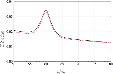
Figure 6: Two-mode diffuson signal $\delta X_{\text{D2}}(t,0)$ in the forward direction relative to the non-pulsed contribution, i.e., half of (42), as function of $t/\tau_{\text{e}}$, after two dephasing pulses at $t_{1}=10\tau_{\text{e}}$ and $t_{2}=40\tau_{\text{e}}$. The black line shows the result of (43), a pronounced echo around $\tau_{3}=60\tau_{\text{e}}$. The red dashed curve shows the analytical approximation, eq. (49), above the background.

As function of $t$ around $\tau_{3}=2(t_{2}-t_{1})$, the signal then is very well approximated by

$$\delta X_{\text{D2}}(t,0) ={2\pi^{d/2}X_{0}\over\pi\nu\hbar(Dt)^{d/2}}\left(\tau_{\text{e}}+|t-\tau_{3}|\right)e^{-|t-\tau_{3}|/\tau_{\text{e}}}.$$ (49)

This echo signal is exponentially suppressed outside the echo time $\tau_{3}=2(t_{2}-t_{1})$, showing a quadratic departure for $|t-\tau_{3}|\ll\tau_{\text{e}}$. At the echo time $t=\tau_{3}$, the signal remains smaller by a factor $\tau_{\text{e}}/t\ll 1$ compared to the non-dephased signal (42). This factor results from phase space reduction: without a field pulse the two diffusons can connect at any time $0<t^{\prime}<t$, while in presence of the two pulses the time $t^{\prime}$ is effectively restricted to an interval of size $\tau_{\text{e}}$ around $t^{\prime}=2t_{1}$.

Figure 6 shows the D2 contrast after two pulses at $t_{1}=10\tau_{\text{e}}$ and $t_{2}=40\tau 2$ with its echo at $\tau_{3}=60\tau_{\text{e}}$, relative to the non-pulsed diffuson signal, i.e., half of (42). Actually, the echo contrast (49) appears on top of a smooth background, created by a combination of a double-pulsed diffuson with a non-pulsed diffuson. These contributions stem from the $t^{\prime}$-integration outside the interval (45) and result in a flat background of the same order than the echo itself. The black line shows the result of the full integration (43), whereas the dashed red line shows the analytical approximation (49) plus the background of unity.

A.2 Two-mode Cooperon C2

Next we turn to the two-mode Cooperon $\delta X_{\text{C2}}(t)$, eq. (IV.4.3). Using the general Cooperon solution (77) and integrating over $\mathbf{q}^{\prime}$ yields

$$\delta X_{\text{C2}}(t,\mathbf{q}) ={2\pi^{d/2}X_{0}\over\pi\nu\hbar(Dt)^{d/2}}\int_{0}^{t}dt^{\prime}\,e^{-\phi_{\text{C2}}(t^{\prime},t,\mathbf{q})},$$ (50)

where the contrast penalty now reads

$$\phi_{\text{C2}}(t^{\prime},t,\mathbf{q}) ={D\over\hbar^{2}}\Big{[}t^{\prime}\left(1-\frac{t^{\prime}}{t}\right)\mathbf{q}^{2}+2\left\{\left(1-\frac{t^{\prime}}{t}\right)\bar{\chi}_{1}(t^{\prime},0,t^{\prime})-\frac{t^{\prime}}{t}\bar{\chi}_{1}(t,t^{\prime},t-t^{\prime})\right\}\mathbf{q}\cdot{\Delta\mathbf{p}}$$

$$\qquad+\left\{\bar{\chi}_{2}(t^{\prime},0,t^{\prime})+\bar{\chi}_{2}(t,t^{\prime},t-t^{\prime})-\tfrac{1}{t}[\bar{\chi}_{1}(t^{\prime},0,t^{\prime})+\bar{\chi}_{1}(t,t^{\prime},t-t^{\prime})]^{2}\right\}{\Delta\mathbf{p}}^{2}\Big{]}.$$ (51)

The principal echo signal stems from the upper configuration in the right panel of Fig. 3, where each Cooperon mode contains exactly one pulse and which is selected by choosing in (50) the integration limits

$$t_{1}<t^{\prime}<t_{2}.$$ (52)

Then, the pulse functions (78) and (79) become

$$\bar{\chi}_{1}(t^{\prime},0,t^{\prime}) =2t_{1}-t^{\prime},$$ (53)

$$\bar{\chi}_{1}(t,t^{\prime},t-t^{\prime}) =2t_{2}-t-t^{\prime},$$ (54)

as well as $\bar{\chi}_{2}(t^{\prime},0,t^{\prime})=|\bar{\chi}_{1}(t^{\prime},0,t^{\prime})|$ and $\bar{\chi}_{2}(t,t^{\prime},t-t^{\prime})=|\bar{\chi}_{1}(t,t^{\prime},t-t^{\prime})|$.

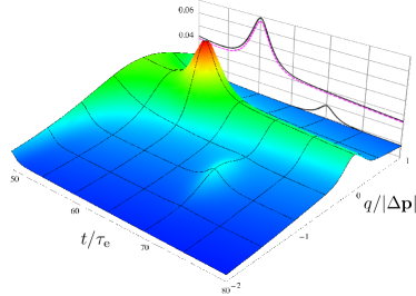
Figure 7: Two-mode echo contrast, eq. (38), relative to the non-pulsed signal (42) as function of $\mathbf{q}\parallel{\Delta\mathbf{p}}$ and $t$ [in units of $\Delta p$ and $\tau_{\text{e}}$] after two dephasing pulses at $t_{1}=10\tau_{\text{e}}$ and $t_{2}=40\tau_{\text{e}}$. The principal echo of processes D2 and C2a appears in the exact forward direction at time $\tau_{3}=2(t_{2}-t_{1})$, whereas the side echo C2b, Eq. (56), appears shifted by ${\Delta\mathbf{p}}$ and at later time $\tau_{4}=2t_{2}-t_{1}$.

Exactly in the forward direction $\mathbf{q}=0$, eq. (A.2) reduces to

$$\phi_{\text{C2}}(t^{\prime},t,0) =\left\{\bar{\chi}_{2}(t^{\prime},0,t^{\prime})+\bar{\chi}_{2}(t,t^{\prime},t-t^{\prime})\right\}/\tau_{\text{e}},$$ (55)

where we have also dropped the last term inside the parentheses multiplying ${\Delta\mathbf{p}}^{2}$, which is small for $\tau_{\text{e}}=\hbar^{2}/(D{\Delta\mathbf{p}}^{2})\ll t$. As function of $t$ around $\tau_{3}=2(t_{2}-t_{1})$, the C2 echo signal is then identical to the D2 signal, eq. (49).

This configuration is, however, not the only possible situation where an echo can arise. Another possibility is shown in the bottom part of the right panel in Fig. 3. This produces an echo at finite momentum $\mathbf{q}=-{\Delta\mathbf{p}}$ shifted slightly from the exact forward direction. The reason is that each Cooperon is peaked at backscattering relative to its incident and final momenta. But when the dephasing pulse hits the first Cooperon near the end, this produces an enhancement at intermediate momentum $\mathbf{k}+\mathbf{k}^{\prime\prime}={\Delta\mathbf{p}}$ (this is already seen in Fig. 5 from the displaced C1 peak just after the first kick). The second Cooperon is hit by the pulse in the center and thus produces the usual backscattering enhancement at $\mathbf{k}^{\prime}+\mathbf{k}^{\prime\prime}=0$. Altogether we expect a peak at $\mathbf{k}^{\prime}=\mathbf{k}-{\Delta\mathbf{p}}$ or indeed $\mathbf{q}=-{\Delta\mathbf{p}}$. Its height is slightly smaller than the principal peak. To a very good approximation, the temporal peak profile is given by

$$\delta X_{\text{C2}}(t,-{\Delta\mathbf{p}}) =\frac{2\pi^{d/2}X_{0}\tau_{\mathrm{e}}}{\pi\nu\hbar(Dt)^{d/2}}h\left(\frac{t-\tau_{4}}{\tau_{\mathrm{e}}}\right)$$ (56)

with $h(s)=\frac{2}{3}\left[2e^{-|s|}-e^{-2|s|}\right]$. Remark that no such configuration is possible for the D2 topology because there the loops are traversed in opposite order, and consequently it is impossible for the pulses to hit only one diffuson mode, but not the other.

Summarizing the double-mode momentum-space discussion, Fig. 7 shows the combined signal, eq. (38), normalized with respect to the unperturbed signal (42).

Appendix B Diffusion modes with dephasing

In this appendix, we solve the generalized diffusion equations, (4) for the quantum diffusion modes in the presence of an external scalar dephasing field (6).

B.1 Diffuson

We start out with the diffuson, for which it is convenient to use central and relative times, $t=(t^{+}+t^{-})/2$, $t^{\prime}=t-T$ and $\eta=t^{+}-t^{-}$, such that

$$t^{\pm}=t\pm\eta/2,\qquad t^{\pm}-T=t^{\prime}\pm\eta/2.$$ (57)

In these variables, the differential equation for the diffuson $\Pi_{\text{D}}(\mathbf{r},\mathbf{r}^{\prime},t^{+},t^{-},T)=D^{\eta}_{tt^{\prime}}(\mathbf{r},\mathbf{r}^{\prime})$ takes the form

$$\left(\partial_{t}-D\partial^{2}_{\mathbf{r}}-i\phi_{-}^{\eta}(\mathbf{r},t)\right)D^{\eta}_{tt^{\prime}}(\mathbf{r},\mathbf{r}^{\prime}) =\delta(t-t^{\prime})\delta(\mathbf{r}-\mathbf{r}^{\prime}).$$ (58)

From here on we use the short notation

$$F_{-}^{\eta}(t) =F\left(t+\frac{\eta}{2}\right)-F\left(t-\frac{\eta}{2}\right)$$ (59)

for arbitrary functions $F(t)$. For the classical diffuson one has $\eta=0$ and thus the dephasing potential $\phi^{0}_{-}=0$ disappears from the problem, as it should. In the generalized diffuson however, particle and hole visit the same position time-shifted by $\eta$, and dephasing occurs.

Eq. (58) is equivalent to the imaginary-time Schrödinger equation for a particle of mass $m=1/2D$ in a scalar potential $i\phi_{-}^{\eta}(\mathbf{r},t)$. Its solution can be written as the path integral Feynman ; EfrosPollack

$$D^{\eta}_{tt^{\prime}}(\mathbf{r},\mathbf{r}^{\prime}) =\int_{\mathbf{r}(t^{\prime})=\mathbf{r}^{\prime}}^{\mathbf{r}(t)=\mathbf{r}}{\cal D}[\mathbf{r}(s)]$$ (60)

$$\times \exp\left(-\int_{t^{\prime}}^{t}ds\left\{{\mathbb{\dot{r}}^{2}(s)\over 4D}+i\phi_{-}^{\eta}(\mathbf{r}(s),s)\right\}\right).$$

We are interested in a potential that describes momentum kicks via a homogeneous force applied at well-defined instances $t_{1},t_{2},...,t_{N}$ in time, $\hbar\phi(\mathbf{r},t)=-\mathbf{r}\cdot\Delta\mathbb{p}f(t)$, where ${\Delta\mathbf{p}}$ is the momentum transferred by a single pulses, and $f(t)$ is a sum of functions peaked at the kick times $t_{i}$. We assume that the individual pulses are short compared to their separation, such that $f(t)$ is zero outside the vicinities $I_{i}$ of the $t_{i}$ and normalized to $\int_{I_{i}}dtf(t)=1$. Aside this constraint, the following solution holds for arbitrary pulse shapes.

To calculate the path integral we decompose the path $\mathbf{r}(s)$ connecting $\mathbf{r}^{\prime}$ to $\mathbf{r}$ in the time $T=t-t^{\prime}$ into a straight, ballistic trajectory plus fluctuations, $\mathbf{r}(s)=\overline{\mathbf{r}}(s)+\widetilde{\mathbf{r}}(s)$. The ballistic path for $t^{\prime}\leq s\leq t$ is $\overline{\mathbf{r}}(s)=\mathbf{r}^{\prime}+\frac{s-t^{\prime}}{T}\Delta\mathbf{r}$, where $\Delta\mathbf{r}=\mathbf{r}-\mathbf{r}^{\prime}$ and the closed loops from $\widetilde{\mathbf{r}}(t^{\prime})=0$ to $\widetilde{\mathbf{r}}(t)=0$ can be written as the Fourier series $\widetilde{\mathbf{r}}(s)={1\over\sqrt{T}}\sum_{n\neq 0}\mathbf{r}_{n}e^{-i\omega_{n}s}$ with $\omega_{n}=2\pi n/T$. Inserting into (60), one notices that the two contributions decouple,

$$D^{\eta}_{tt^{\prime}}(\mathbf{r},\mathbf{r}^{\prime}) =\overline{D}^{\eta}_{tt^{\prime}}(\mathbf{r},\mathbf{r}^{\prime})\widetilde{D}^{\eta}_{tt^{\prime}}.$$ (61)

Only the ballistic contribution depends on the positions,

$$\overline{D}^{\eta}_{tt^{\prime}}(\mathbf{r},\mathbf{r}^{\prime}) =\exp\left(-{\Delta\mathbf{r}^{2}\over 4DT}+i{{\Delta\mathbf{p}}\over\hbar}\cdot\int_{t^{\prime}}^{t}ds\,\overline{\mathbf{r}}(s)f_{-}^{\eta}(s)\right),$$ (62)

where the $s$-independent components of $\overline{\mathbf{r}}(s)$ are weighted by the number

$$\chi_{0}^{\eta}(t^{\prime},t) =\int_{t^{\prime}}^{t}dsf_{-}^{\eta}(s).$$ (63)

This is essentially the difference in the number of kicks experienced by particle and hole during their evolution over the interval $[t^{\prime}\pm\frac{\eta}{2},t\pm\frac{\eta}{2}]$, respectively. For the classical diffuson with $\eta=0$, these numbers are of course equal, and thus $\chi^{0}_{0}(t^{\prime},t)=0$. A priori, this need not be the case in the general setting. If, then, particle and hole do not experience the same number of kicks, this will result in uncompensated phases at all times. Therefore, we will consider in the following only those cases where particle and hole experience the same number of kicks (but possibly at different times), and correspondingly make use of $\chi_{0}^{\eta}(t^{\prime},t)=0$.

As a consequence, Eq. (62) depends only on the position difference,

$$\overline{D}^{\eta}_{tt^{\prime}}(\Delta\mathbf{r}) =\exp\left(-{\Delta\mathbf{r}^{2}\over 4DT}+i\frac{\chi_{1}^{\eta}(t^{\prime},t)}{T\hbar}{\Delta\mathbf{p}}\cdot\Delta\mathbf{r}\right),$$ (64)

where the function

$$\chi_{1}^{\eta}(t^{\prime},t) =\int_{t^{\prime}}^{t}ds\,s\,f_{-}^{\eta}(s)$$ (65)

essentially evaluates the differences in particle and hole kick times. Fourier transformation in $\Delta\mathbf{r}$ then results in

$$\overline{D}^{\eta}_{tt^{\prime}}(\mathbb{q}) =\mathcal{N}^{-1}\exp\left(-\frac{D}{T\hbar^{2}}\left[T\mathbf{q}-\chi_{1}^{\eta}(t^{\prime},t){\Delta\mathbf{p}}\right]^{2}\right),$$ (66)

with normalization ${\cal N}=(4\pi DT)^{-d/2}$.

Concerning the fluctuations, Gaussian integration over the $\mathbf{r}_{n}$ contributes the position-independent, but time-dependent contrast factor

$$\widetilde{D}^{\eta}_{tt^{\prime}} =\mathcal{N}\exp\left[-{D{\Delta\mathbf{p}}^{2}\over\hbar^{2}}\left(\chi_{2}^{\eta}(t^{\prime},t)-{\chi_{1}^{\eta}(t^{\prime},t)^{2}\over T}\right)\right],$$ (67)

where $\chi_{1}^{\eta}(t^{\prime},t)$ of (65) appears squared, and

$$\chi_{2}^{\eta}(t^{\prime},t) =-\frac{1}{2}\int_{t^{\prime}}^{t}ds_{1}\int_{t^{\prime}}^{t}ds_{2}\,|s_{1}-s_{2}|f_{-}^{\eta}(s_{1})f_{-}^{\eta}(s_{2}).$$ (68)

When deriving the above expressions we have used that Gaussian integration over the $\mathbf{r}_{n}$ contributes the position-independent, but time-dependent contrast factor

$$\widetilde{D}^{\eta}_{tt^{\prime}} ={\cal N}\exp\left[-{D{\Delta\mathbf{p}}^{2}\over T\hbar^{2}}\sum_{n\neq 0}{{\cal F}_{n}^{\eta}(t^{\prime},t){\cal F}_{-n}^{\eta}(t^{\prime},t)\over\omega_{n}^{2}}\right],$$ (69)

where we introduced the pulse-difference Fourier transform ${\cal F}_{n}^{\eta}(t^{\prime},t)=\int_{t^{\prime}}^{t}ds\,e^{-i\omega_{n}s}f_{-}^{\eta}(s)$. The sum over frequencies in (69) is readily performed using that

$$\sum_{n\neq 0}{e^{i\omega_{n}\Delta s}\over\omega_{n}^{2}} ={T^{2}\over 12}-\frac{T|\Delta s|}{2}+{\Delta s^{2}\over 2},$$ (70)

with $\Delta s=s_{1}-s_{2}$, and upon employing $\chi_{0}^{\eta}(t^{\prime},t)=0$ (see discussion below eq. (63)) one arrives at the stated result.

Summarizing we find the general diffuson

$$\Pi_{\text{D}}(\mathbf{q},t^{+},t^{-},T)=e^{-{D\over\hbar^{2}}\left[T\mathbf{q}^{2}-2\chi_{1}(t^{+},t^{-},T)\mathbf{q}\cdot{\Delta\mathbf{p}}+\chi_{2}(t^{+},t^{-},T){\Delta\mathbf{p}}^{2}\right]},$$ (71)

where we returned to the time variables $t^{\pm},T$ introduced in the main text, and defined

$$\chi_{1} (t^{+},t^{-},T)=\int_{-T}^{0}ds\,s\left[f(s+t^{+})-f(s+t^{-})\right]$$

$$=\int ds\,f(s)\left[(s-t^{+})\chi_{T}^{+}(s)-(s-t^{-})\chi_{T}^{-}(s)\right],$$ (72)

with $\chi_{T}^{\pm}(s):=\chi_{[-T,0]}(s-t^{\pm})$ the characteristic function of the time interval $[-T,0]$, evaluated for the particle at $s-t^{+}$ and the hole at $s-t^{-}$. Similarly,

$$\chi_{2} (t^{+},t^{-},T)=-\frac{1}{2}\int ds_{1}\int ds_{2}f(s_{1})f(s_{2})$$

$$\times\Big{[}|s_{1}-s_{2}|\left\{\chi_{T}^{+}(s_{1})\chi_{T}^{+}(s_{2})+\chi_{T}^{-}(s_{1})\chi_{T}^{-}(s_{2})\right\}$$

$$\qquad-2|s_{1}-t^{+}-s_{2}+t^{-}|\chi_{T}^{+}(s_{1})\chi_{T}^{-}(s_{2})\Big{]}.$$ (73)

Specialized to $\delta$-pulses $t_{1}$ and $t_{2}$ the above expressions turn into eqs. (46) and following used in section A.1.

B.2 Cooperon

Turning to the Cooperon, it is again convenient to use central and relative times, $t=(t^{+}+t^{-})/2$ and $\eta=t^{+}-t^{-}$, as well as $\eta-\eta^{\prime}={\Delta\eta}=2T$, such that

$$t^{\pm}=t\pm\eta/2,\qquad t^{\pm}\mp T=t\pm\eta^{\prime}/2.$$ (74)

In these variables, the Cooperon differential equation for $\Pi_{\text{C}}(\mathbf{r},\mathbf{r}^{\prime},t^{+},t^{-},T)=C^{t}_{\eta\eta^{\prime}}(\mathbf{r},\mathbf{r}^{\prime})$ takes the form

$$\left(\partial_{\eta}-\frac{D}{2}\partial^{2}_{\mathbf{r}}-\frac{i}{2}\phi_{-}^{\eta}(\mathbf{r},t)\right)C^{t}_{\eta\eta^{\prime}}(\mathbf{r},\mathbf{r}^{\prime}) =\delta(\eta-\eta^{\prime})\delta(\mathbf{r}-\mathbf{r}^{\prime}),$$ (75)

where $\phi_{-}^{\eta}(t)=\phi(t+\frac{\eta}{2})-\phi(t-\frac{\eta}{2})$ as before. For the single-mode Cooperon, equality of starting and end times imposes $\eta^{\prime}=-\eta$. In difference to the diffuson case, the dephasing potential stays in the problem, and we now have to solve the equation of motion in $\eta$ at fixed $t$. This is achieved with the path integral Feynman ; EfrosPollack

$$C^{t}_{\eta\eta^{\prime}}(\mathbf{r},\mathbf{r}^{\prime}) =\int_{\mathbf{r}(\eta^{\prime})=\mathbf{r}^{\prime}}^{\mathbf{r}(\eta)=\mathbf{r}}{\cal D}[\mathbf{r}(u)]$$ (76)

$$\times \exp\left(-\int_{\eta^{\prime}}^{\eta}du\left\{{\mathbb{\dot{r}}^{2}(u)\over 2D}+\frac{i}{2}\phi_{-}^{u}(\mathbf{r}(u),t)\right\}\right).$$

Following then the same steps as before for the diffuson one arrives at the dephased general Cooperon (expressed in time variables $t^{\pm},T$ used in the main text)

$$\Pi_{\text{C}}(\mathbf{q},t^{+},t^{-},T) =e^{-{D\over\hbar^{2}}\left[T\mathbf{q}^{2}-2\bar{\chi}_{1}(t^{+},t^{-},T)\mathbf{q}\cdot{\Delta\mathbf{p}}+\bar{\chi}_{2}(t^{+},t^{-},T){\Delta\mathbf{p}}^{2}\right]},$$ (77)

where

$$\bar{\chi}_{1}(t^{+},t^{-},T)=\int du\,f(u)\left[(u-t^{+})\bar{\chi}_{T}^{+}(u)+(u-t^{-})\bar{\chi}_{T}^{-}(u)\right],$$ (78)

with $\bar{\chi}_{T}^{\pm}(u):=\chi_{[-T,0]}(\pm(u-t^{\pm}))$ the characteristic function of the time interval $[-T,0]$, evaluated for the particle at $u-t^{+}$ and the hole at $t^{-}-u$. Similarly,

$$\bar{\chi}_{2} (t^{+},t^{-},T)=-\frac{1}{2}\int du_{1}\int du_{2}f(u_{1})f(u_{2})$$

$$\times\Big{[}|u_{1}-u_{2}|\left\{\bar{\chi}_{T}^{+}(u_{1})\bar{\chi}_{T}^{+}(u_{2})+\bar{\chi}_{T}^{-}(u_{1})\bar{\chi}_{T}^{-}(u_{2})\right\}$$

$$\quad-2|u_{1}+u_{2}-t^{+}-t^{-}|\bar{\chi}_{T}^{+}(u_{1})\bar{\chi}_{T}^{-}(u_{2})\Big{]}.$$ (79)

The single-mode Cooperon evaluated at $t^{+}=t=T$ and $t^{-}=0$ then reads

$$\Pi_{\text{C}}(\mathbf{q},t) =e^{-{D\over\hbar^{2}}\left[t\mathbf{q}^{2}-2\bar{\chi}_{1}(t)\mathbf{q}\cdot{\Delta\mathbf{p}}+\bar{\chi}_{2}(t){\Delta\mathbf{p}}^{2}\right]},$$ (80)

where the auxiliary functions in the exponential are

$$\bar{\chi}_{1}(t) =\int_{0}^{t}du(2u-t)f(u),$$ (81)

$$\bar{\chi}_{2}(t) =\int_{0}^{t}du\int_{0}^{t}dvf(u)f(v)(|u+v-t|-|u-v|).$$ (82)

For a single $\delta$-pulse $f(t)=\delta(t-t_{1})$, these functions become $\bar{\chi}_{1}(t)=(2t_{1}-t)\theta(t-t_{1})$, and $\bar{\chi}_{2}(t)=|2t_{1}-t|\theta(t-t_{1})$ as used in section III. From the general expressions (81) and (82) we further find the features also discussed there, i.e. for a pulse of finite resolution in time but still symmetric around $t_{1}$, $\int dt\,t\,f(t)=\langle t\rangle_{f}=t_{1}$ defines the dephasing pulse center, and thus $\bar{\chi}_{1}(2t_{1})=0$ by construction. At this instant, the entire contrast penalty vanishes, since $\bar{\chi}_{2}(t)$ vanishes by symmetry as well, implying a perfect revival. Only for an asymmetric pulse the contrast penalty will generically remain finite, since then $\bar{\chi}_{2}(t)$ is not required to vanish exactly at $2t_{1}$, and the echo will appear with reduced contrast. Finally, for a sequence of two $\delta$-kicks

$$\bar{\chi}_{1}(t) =2(t_{1}+t_{2}-t),$$ (83)

$$\bar{\chi}_{2}(t) =|2t_{1}-t|+|2t_{2}-t|+2|t_{1}+t_{2}-t|-2|t_{2}-t_{1}|,$$ (84)

which results in a C1 echo at time $\tau_{2}=t_{1}+t_{2}$.

References

- (1) 50 Years of Anderson Localization, E. Abrahams ed. (World Scientific, Singapore, 2010).
- (2) D. S. Wiersma, P. Bartolini, A. Lagendijk, R. Righini, Nature 390, 671 (1997).
- (3) T. Sperling, W. Bührer, C. M. Aegerter, and G. Maret, Nature Photon. 7, 48 (2013).
- (4) A. A. Chabanov, M. Stoytchev, and A. Z. Genack, Nature 404, 850 (2000).
- (5) P. W. Anderson, Phys. Rev. 109,1492 (1958).
- (6) J. Chabé, et al., Phys. Rev. Lett. 101, 255702 (2008).
- (7) J. Billy, V. Josse, Z. Zuo, A. Bernard, B. Hambrecht, P. Lugan, D. Clément, L. Sanchez-Palencia, P. Bouyer and A. Aspect, Nature 453, 891 (2008).
- (8) G. Roati, C. D’Errico, L. Fallani, M. Fattori, C. Fort, M. Zaccanti, G. Modugno, M. Modugno, M. Inguscio, Nature 453, 895 (2008).
- (9) S. S. Kondov, W. R. McGehee, J. J. Zirbel, B. DeMarco, Science 334, 66 2011.
- (10) F. Jendrzejewski, A. Bernard, K. Müller, P. Cheinet, V. Josse, M. Piraud, L. Pezzé, L. Sanchez-Palencia, A. Aspect, P. Bouyer, Nat. Phys. 8, 398 (2012).
- (11) G. Semeghini, M. Landini, P. Castilho, S. Roy, G. Spagnolli, A. Trenkwalder, M. Fattori, M. Inguscio, and G. Modugno, arXiv:1404.3528.
- (12) T. Schwartz, G. Bartal, S. Fishman, M. Segev, Nature 446, 52 (2007).
- (13) Y. Lahini, A. Avidan, F. Pozzi, M. Sorel, R. Morandotti, D. N. Christodoulides, and Y. Silberberg Phys. Rev. Lett. 100, 013906 (2008).
- (14) H. Hu, A. Strybulevych, J. H. Page, S. E. Skipetrov, B. A. van Tiggelen, Nat. Phys. 4, 945 (2008).
- (15) E. Akkermans and G. Montambaux, Mesoscopic Physics of Electrons and Photons (Cambridge Univ. Press, 2006).
- (16) T. Karpiuk, N. Cherroret, K. L. Lee, B. Grémaud, C. A. Müller, C. Miniatura, Phys. Rev. Lett. 109, 190601 (2012).
- (17) T. Micklitz, C. A. Müller, A. Altland, Phys. Rev. Lett. 112, 110602 (2014).
- (18) K. L. Lee, B. Grémaud, C. Miniatura, Phys. Rev. A 90, 043605 (2014).
- (19) S. Ghosh, N. Cherroret, B. Grémaud, C. Miniatura, D. Delande, Phys. Rev. A 90, 063602 (2014).
- (20) N. Cherroret, T. Karpiuk, C. A. Müller, B. Grémaud, C. Miniatura, Phys. Rev. A 85, 011604(R) (2012).
- (21) F. Jendrzejewski, K. Müller, J. Richard, A. Date, T. Plisson, P. Bouyer, A. Aspect, V. Josse, Phys. Rev. Lett. 109, 195302 (2012).
- (22) A. Altland and B. Simons, Condensed Matter Field Theory (Cambridge Univ. Press, 2007).
- (23) B. L. Altshuler, A. G. Aronov, Electron-Electron Interaction in Disordered Systems (Eds. A. L. Efros, M. Pollak), pp. 1-153 North-Holland, Amsterdam (1985).
- (24) R. P. Feynman and A. R. Hibbs, Quantum Mechanics and Path Integrals, (New York: McGraw-Hill 1965).
- (25) G. Labeyrie, T. Karpiuk, J.-F. Schaff, B. Grémaud, C. Miniatura, D. Delande, Europhys. Lett. 100, 66001 (2012).
- (26) N. Cherroret and D. Delande, Phys. Rev. A, 88, 035602 (2013).
- (27) T. Engl, J. Dujardin, A. Argüelles, P. Schlagheck, K. Richter, J. D. Urbina, Phys. Rev. Lett., 112, 140403, (2014).
- (28) K. B. Efetov, Supersymmetry in Disorder and Chaos (Cambridge U. Press, 1999).
- (29) A. Kamenev, A. Andreev, Phys.Rev. B 60, 2218 (1999).
- (30) A. Kamenev, A. Levchenko, Advances in Physics 58, 197 (2009).
- (31) A. Altland, A. Kamenev, Phys. Rev. Lett. 85, 5615 (2000).
- (32) T. Plisson, T. Bourdel, C. A. Müller, Eur. J. Phys. ST 217, 79 (2013).
- (33) K. Müller, J. Richard, V. Volchkov, V. Denechaud, P. Bouyer, A. Aspect, V. Josse, arXiv:1411.1671.
- (34) T. Engl, J.-D. Urbina, K. Richter, arXiv:1409.5684.
- (35) M. Serbyn, M. Knap, S. Gopalakrishnan, Z. Papić, N. Y. Yao, C. R. Laumann, D. A. Abanin, M. D. Lukin, and E. A. Demler, Phys. Rev. Lett. 113, 147204 (2014).