Renormalization of a one-parameter family of piecewise isometries

Abstract

We consider a one-parameter family of piecewise isometries of a rhombus. The rotational component is fixed, and its coefficients belong to the quadratic number field $K=\mathbb{Q}(\sqrt{2})$. The translations depend on a parameter $s$ which is allowed to vary in an interval. We investigate renormalizability. We show that recursive constructions of first-return maps on a suitable sub-domain eventually produce a scaled-down replica of this domain, but with a renormalized parameter $r(s)$. The renormalization map $r$ is the second iterate of a map $f$ of the generalised Lüroth type (a piecewise-affine version of Gauss’ map). We show that exact self-similarity corresponds to the eventually periodic points of $f$, and that such parameter values are precisely the elements of the field $K$ that lie in the given interval.

The renormalization process is organized by a graph analogous to those used to construct renormalizable interval-exchange transformations. There are ten distinct renormalization scenarios corresponding to as many closed circuits in the graph. The process of induction along some of these circuits involves intermediate maps undergoing, as the parameter varies, infinitely many bifurcations.

Our proofs rely on computer-assistance.

1 Introduction

In piecewise isometries (PWI), renormalizability is a key for a complete description of the dynamics. The phase space of these systems is partitioned into domains, called atoms, over each of which the dynamics is an isometry. By choosing a sub-domain of the original space —typically an atom or a union of atoms— and considering the first-return map to it, one constructs a new system, the induced PWI on the chosen domain. If this process is repeated, then it may happen that an induced system be conjugate to the original system. This circumstance usually leads to a detailed understanding of the dynamics.

In one-dimension (interval-exchange transformations —IET) there is a satisfactory theory of renormalization. The Rauzy induction gives a criterion for selecting an interval (not one of the atoms) over which to induce, resulting in a new IET with the same number of atoms [19, 22]. This induction process is a dynamical system over a finite-dimensional space of IETs, related to the continued fractions algorithm, which affords a good description of the parameter space of IETs [23].

An important connection with Diophantine arithmetic is provided by the Boshernitzan and Carrol theorem [4]; it states that in any IET defined over a quadratic number field, inducing on any of the atoms results in only finitely many distinct IETs, up to scaling. For a two-interval exchange, this finiteness result reduces to Lagrange’s theorem on the eventual periodicity of the continued fractions expansions of quadratic surds. Furthermore, if a (uniquely ergodic) IET is renormalizable, then the scaling constant involved in renormalization is a unit in a distinguished ring of algebraic integers [18].

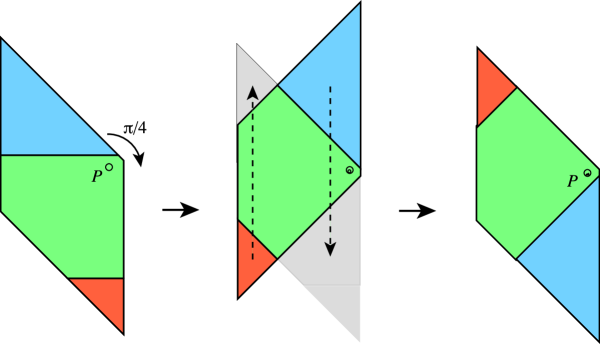
Figure 1: Our model: a rhombus $\mathrm{R}$ with vertex angle $\pi/4$ is rotated clockwise by $\pi/4$ about a parameter-dependent fixed point $P$ located on the short diagonal. This leaves two triangular pieces outside the boundary of $\mathrm{R}$. These are translated vertically back into $\mathrm{R}$ to complete the piecewise isometry.

In two dimensions general results are scarce [16, 17]. Until recently detailed results on renormalization were limited to special cases, defined over quadratic number fields [13, 1, 11, 2, 20]. These results point consistently towards the existence of a two-dimensional analogue of the B&C theorem. A more intricate form of renormalization has also been found in a handful of cubic cases [9, 14]. In all cases, the renormalization constants are units in the ring of integers of the field of definition of the PWI.

More recently, renormalization has been studied in parametrised families. Hooper considered a two-parameter family of rectangle exchange transformations, and used techniques connected to the renormalization of Truchet tilings to establish results on the measure of the periodic and aperiodic sets of the map [10]. In a substantial monograph [21], Schwartz determined the renormalization group of a one-parameter family of polygon-exchange transformations, where the exchange is achieved by translations only. In this model, inducing on suitable domains leads to a conjugacy of the map to its inverse, accompanied by a change of parameter given by a piecewise-Möbius map (a variant of Gauss’ map). Metric and topological properties of the limit set are also established.

In the present work we consider a family of PWIs of a rhombus $\mathrm{R}$ with rotation angle $-\pi/4$ and a fixed point $P$ which is allowed to vary along the short diagonal, controlled by a real parameter $s$ (see figure 1). The choice of rotation determines the quadratic number field $\mathbb{Q}(\sqrt{2})$. Some special parameter values in this field ($s=0,1+\sqrt{2},2(1+\sqrt{2}))$ have received much attention [1, 11, 2]; they correspond to $P$ being the centre and a vertex of the rhombus. These PWIs show exact self-similarity, and, as a result, their dynamics is well-understood.

For all maps in our family, the edges of the atoms have normal vectors in $\mathbb{Q}(\sqrt{2})^{2}$, while the Cartesian coordinates of the vertices belong to $\mathbb{Q}(\sqrt{2})+\mathbb{Q}(\sqrt{2})s$, which is a two-dimensional vector space over $\mathbb{Q}(\sqrt{2})$. The same is true of the first-return map induced on any of the atoms, and recursively, of any higher-level induced return maps. This arithmetical environment will have a profound effect on the renormalization.

We have two main results, theorems 1 and 2, stated in section 4. In theorem 1 we prove that the parametrised rhombus map, restricted to the parameter interval $s\in I=[0,\sqrt{2}]$, induces in one of its triangular atoms a renormalizable five-atom PWI, i.e., one which, after repeated inductions, recurs at smaller length scales with a piecewise-affine change of parameter $s\mapsto r(s)$. We show that $r$ is the second iterate of a modified Lüroth map $f$ (a piecewise affine version of the Gauss map for continued fractions), which is shown in figure 2. We also show that all scaling constants are units in the ring $\mathbb{Z}[\sqrt{2}]$.

Exact self-similarity is achieved if the induction process eventually reproduces a value of $s$ which has already been encountered, i.e., if $s$ is an eventually periodic point of $r$. In theorem 2 we prove that these parameter values are precisely the elements of $\mathbb{Q}(\sqrt{2})\cap I$. Note that, unlike the classic case of continued fractions, here eventual periodicity is associated with a single quadratic field. This arithmetical characterisation of renormalizability provides additional evidence for the existence of an analogue of the B&C theorem for polygon-exchange transformations.

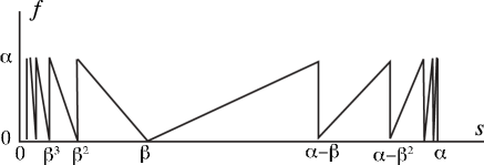
Figure 2: The piecewise-affine renormalization function $f$ which controls the renormalization of the piecewise isometry $\rho=\rho(s)$ defined in section 3. Here $\alpha=\sqrt{2}$, $\beta=\alpha-1$, and the function $f$ maps the parametric interval $I=[0,\alpha)$ into itself.

The discontinuities of the function $r$ accumulate at the infinitely many zeros of $f$ (see figure 7). As a result, the return-map dynamics is highly non-uniform, with ever-increasing return times as $s$ approaches such discontinuities. The number of qualitatively distinct renormalization scenarios can be reduced to ten. The simplest of these involves a single induction, and it applies to the case in which both $s$ and $f(s)$ are in the middle of the interval $I$ .

At the opposite extreme are, among others, those parts of $I$ for which both $s$ and $\sqrt{2}-f(s)$ are small. As a preview of renormalization dynamics, let us briefly sketch this scenario, represented schematically in figure 3. In this scheme, the number of inductions remains fixed at six, and it involves the same types of induced PWIs (the pencil, the fringed triangle, and the double strip). For either $s$ or $f(s)$ approaching zero or $\sqrt{2}$, the numbers of atoms increases without bounds, but in a tightly controlled manner (the complexity increases logarithmically). The return times are are also unbounded.

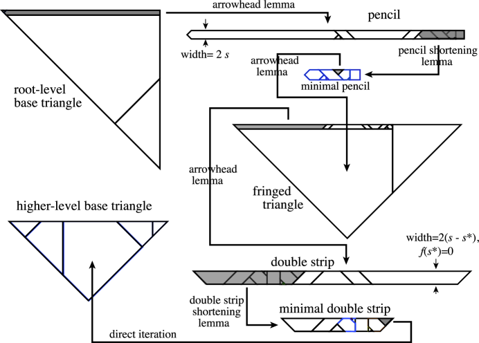
Figure 3: Sketch of the renormalization scenario for $s$ close to 0 and $f(s)$ close to $\sqrt{2}$. In the figure, the relative sizes of the various objects are greatly distorted in order to reveal their structure.

The map $f$ serves as a phase function for the evolution of the pencil with decreasing $s$, with two new atoms emerging at the boundary whenever $f(s)$ passes through unity. Analogously, bifurcations of the double strip occur at the zeros of $r(s)$. The spatial scaling accompanying the renormalization is governed by the successive narrowing of the widths of the pencil and the double strip.

Of the six induction steps, two are ‘shortenings’, exploiting the repetitive, quasi-one-dimensional structures of pencils and double strips. Steps 1, 3, and 4 appear to be more complicated, but in fact are all grounded in one simple dynamical sub-system, the arrowhead. Once we have formulated that underlying dynamics in the Arrowhead Lemma of section 9, all aforementioned induction steps can be split into two manageable parts: the first, with short, fixed-length return orbits which can be constructed by explicit iteration, and the second, in which the Arrowhead Lemma accounts for all of the $s$-dependent bifurcations.

1.1 Structure of the paper

Sections 2–4: Preliminaries, and formulation of the main results

In section 2 we provide definitions and notation which will be used throughout, followed by the specification of our model in section 3. In section 4 we define the renormalization function $f$ and $r$ and state our two main theorems. The first of these, theorem 1, describes the renormalization of our central geometric structure, the two-parameter base triangle with its five-atom piecewise isometry. The second, theorem 2, introduces the symbolic dynamics of the renormalization and establishes the connection between exact self-similarity and membership in the field $\mathbb{Q}(\sqrt{2})$.

Sections 5,6: Symbolic dynamics, Lüroth expansion, proof of theorem 2

After introducing a symbolic representation of parameter space in section 5, we derive the Lüroth expansion and prove theorem 2 using a contraction argument on a lattice.

Section 7: Renormalization overview

Here we provide roadmaps for navigating the rest of the paper, organized around a renormalization graph, analogous to the Rauzy graphs of interval exchange theory [19]. Oriented edges of the graph correspond to various return-map inductions, and closed circuits describe the ten distinct pathways by which one succeeds in renormalizing the initial base triangle on various subsets of the parameter interval $I$.

Sections 8,9: Machinery for proving theorem 1

In section 8 we define the parametric dressed domains (tiled polygons with associated piecewise isometries) which correspond to the vertices of the renormalization graph: the pencil, the fringed triangle, and the double strip. In addition, we prove two Shortening Lemmas which allow one to reduce pencils and double strips to their minimum lengths. Section 9 is devoted to the arrowhead and its dynamics, culminating in the Arrowhead Lemma.

Section 10: Proof of theorem 1

Through a sequence of propositions, we treat all of the various induction steps needed to prove theorem 1 over the entire interval $I$. Some of the induction steps require only explicit iteration of PWIs over short orbits of fixed length, while others require, in addition, application of one of the Shortening Lemmas or the Arrowhead Lemma.

Section 11: Temporal scaling and fractal structure

As a by-product of section 10, we obtain the incidence matrices which determine the renormalization’s return times and asymptotic temporal scaling. We obtain explicit formulae for these matrices in section 11, where we also explore briefly the implications for the $s$-dependence of the Hausdorff dimension of the exceptional set.

Many steps in the proofs have required computer assistance, invariably to verify statements concerning finite orbits of PWIs. This requires geometrical transformations of polygons (translations, rotations, reflections, etc.), polygon inclusion and disjointness tests, plus a fair amount of book-keeping. All arithmetic is performed exactly in $\mathbb{Q}(\sqrt{2})$ and $\mathbb{Q}(\sqrt{2})+\mathbb{Q}(\sqrt{2})s$. The complexity of the computation is manageable, because all of the heavy lifting is taken care by the Arrowhead and Shortening lemmas, which are proved analytically. A complete description and listing of our procedures, in the form of Mathematica^®functions, together with all of the calculations participating in the proof of theorem 1, may be found in the Electronic Supplement [6].

Acknowledgements: JHL and FV would like to thank, respectively, the School of Mathematical Sciences at Queen Mary, University of London, and the Department of Physics of New York University, for their hospitality.

2 Definitions and notation

Throughout this article we adopt the notation

$$\alpha=\sqrt{2},\quad\beta=\sqrt{2}-1,\quad\omega=\sqrt{2}+1.$$

The arithmetical environment is the algebraic number field $\mathbb{Q}(\alpha)$ with its ring of integers $\mathbb{Z}[\alpha]$, given by

$$\mathbb{Q}(\alpha)=\{x+y\alpha\,:\,x,y\in\mathbb{Q}\},\qquad\mathbb{Z}(\alpha)=\{m+n\alpha\,:\,m,n\in\mathbb{Z}\}.$$ (1)

The number $\omega$, which will be shown to determine the scaling, is the fundamental unit in $\mathbb{Z}[\alpha]$ (see [5, chapter 6]). Note that $\beta=\omega^{-1}$ is also a unit.

Our system depends on a parameter $s$, and to represent parameter dependence we consider the set

$${\mathbb{S}}=\mathbb{Q}(\alpha)+\mathbb{Q}(\alpha)s$$ (2)

Here, and below, $s$ is regarded as an indeterminate; hence the set ${\mathbb{S}}$ is a two-dimensional vector space over $\mathbb{Q}(\alpha)$ (a $\mathbb{Q}(\alpha)$-module) whose elements are degree-one polynomials in $s$.

2.1 Planar objects

A tile is an open convex polygon whose edges have outward normal vectors taken from the set $\{\mathbf{u}_{m}=(\cos{m\pi/4},\sin{m\pi/4}):m=0,\ldots,7\}$. The equations of the edges of an $n$-sided tile are thus of the form

$$\mathbf{u}_{m_{i}}\cdot(x,y)=b_{i},\quad i=1,\ldots,n,$$

where the ‘octagonal coordinates’ $b_{i}$ belong to $\mathbb{S}$. The parameter $s$ allows for the continuous deformation of tiles.

We represent an $n$-sided tile $X$ with edge orientations $m_{1},\ldots,m_{n}$ and octagonal coordinates $b_{1},\ldots,b_{n}$ with the bracket notation

$$X=[(m_{1},\ldots,m_{n}),(b_{1},\ldots,b_{n})].$$ (3)

Tile names will always be capital italic letters.

A domain is a union of open polygons whose edges are specified by octagonal orientations $\mathbf{u}_{m}$ and coordinates in the module $\mathbb{S}$. The polygons need not be convex. Domain names will always be capital Roman letters.

A tiling ${\bf X}$ is a set of tiles,

$${\bf X}=\{X_{1},\ldots,X_{n}\}.$$

A tiling ${\bf X}$ is always associated with a domain ${\rm X}$, the span of ${\bf X}$ ,

$${\rm X}={\rm span}({\bf X})\stackrel{{\scriptstyle\rm def}}{{=}}{\rm Int}(\overline{\cup_{i=1}^{n}X_{i}}).$$

The union of two tilings is a tiling.

2.2 Isometry group

We employ a group $\mathfrak{G}$ of transformations of planar objects, to specify their locations and orientations, and to describe their dynamical evolution. The group comprises the rotations and reflections of the symmetry group of the regular octagon (the dihedral group $D_{8}$) together with translations in $\mathbb{S}^{2}$. We define $\mathfrak{G}_{+}$ to be the subgroup of orientation-preserving transformations in $\mathfrak{G}$, i.e., those with Jacobian determinant equal to $+1$.

We adopt the following notation:

• $\mathtt{U}_{n}$: reflection about the lines generated by the extended set of vectors

  $$\mathbf{u}_{k}=(\cos(k\pi/4),\sin(k\pi/4)),\quad k=0,\frac{1}{2},1,\frac{3}{2},\ldots,$$

  where we allow for half-integer indices, to be taken modulo 8;

• $\mathtt{R}_{n}$: rotation by the angle $n\pi/4,\;n=0,\ldots,7$;

• $\mathtt{T}_{\bf d}$: translation by ${\bf d}\in\mathbb{S}^{2}$.

Thanks to the product formulae

$$\mathtt{T}_{\bf d}\mathtt{T}_{\bf e}=\mathtt{T}_{{\bf d}+{\bf e}},\qquad\mathtt{R}_{m}\mathtt{R}_{n}=\mathtt{R}_{m+n},\qquad\mathtt{U}_{m}\mathtt{U}_{n}=\mathtt{R}_{2(m-n)},$$

and commutation relations

$$\mathtt{R}_{n}\mathtt{T}_{\bf d}=\mathtt{T}_{\mathtt{R}_{n}{\bf d}}\mathtt{R}_{n},\qquad\mathtt{R}_{n}\mathtt{U}_{m}=\mathtt{U}_{m+n}\mathtt{R}_{n},\qquad\mathtt{U}_{n}\mathtt{T}_{\bf d}=\mathtt{T}_{\mathtt{U}_{n}{\bf d}}\mathtt{U}_{n},$$ (4)

we can write an arbitrary element $\mathtt{G}$ of ${\mathfrak{G}}$ in the canonical form

$$\mathtt{G}_{n,m,{\bf d}}=\mathtt{T}_{\bf d}\mathtt{R}_{m}\mathtt{U}^{n}_{0},$$

with

$$n\in\{0,1\},\quad m\in\{0,1,\ldots,7\},\quad\mathbf{d}\in\mathbb{S}^{2}.$$

In general, we will write $\mathcal{X}\sim\mathcal{Y}$ to indicate that $\mathcal{X}=\mathtt{G}(\mathcal{Y})$ for some $\mathtt{G}\in\mathfrak{G}$. As $\mathfrak{G}$ is a group, this is an equivalence relation. An equivalence class consists of planar objects which are congruent (same shape and size) up to a reflection. Appendix A contains a catalogue of standard representatives of equivalence classes, used extensively in this work.

2.3 Dressed domains and subdomains

We define a dressed domain to be a triple

$$\mathcal{X}=({\mathrm{X},\mathbf{X},\rho}),$$ (5)

where $\mathrm{X}$ is a domain, $\mathbf{X}$ is a tiling with span $\mathrm{X}$, and $\rho$ is a mapping which acts on each element of $\mathbf{X}$ as an isometry in $\mathfrak{G}_{+}$. We will describe $\rho$ as a piecewise isometry or domain map acting on $\mathrm{X}$, with $\mathbf{X}$ comprising the set of its atoms. Dressed domains will always be denoted by capital script letters. Under the action of an isometry $\mathtt{G}\in\mathfrak{G}$, a dressed domain transforms as

$$\mathtt{G}(\mathcal{X})=\mathtt{G}({\mathrm{X},\mathbf{X},\rho})=(\mathtt{G}(\mathrm{X}),\{\mathtt{G}(X_{1}),\mathtt{G}(X_{2}),\ldots\},\mathtt{G}\circ\rho\circ\mathtt{G}^{-1}).$$

To emphasize the association of a mapping $\rho$ with a particular dressed domain $\mathcal{X}$, we will use the notation $\rho_{\stackrel{{\scriptstyle}}{{\mathcal{X}}}}$.

Let $\mathcal{X}=(\mathrm{X},\mathbf{X},\rho_{\stackrel{{\scriptstyle}}{{\mathcal{X}}}})$ be a dressed domain, and let $\mathrm{Y}$ be a sub-domain of $\mathrm{X}$. We denote by $\rho_{\stackrel{{\scriptstyle}}{{\mathcal{Y}}}}$ the first-return map on $\mathrm{Y}$ induced by $\rho_{\stackrel{{\scriptstyle}}{{\mathcal{X}}}}$. We call the resulting dressed domain $\mathcal{Y}=(\mathrm{Y},\mathbf{Y},\rho_{\stackrel{{\scriptstyle}}{{\mathcal{Y}}}})$ a dressed subdomain of $\mathcal{X}$, writing

$$\mathcal{X}\rightarrow\mathcal{Y}.$$ (6)

A prototype is a canonical representative of an equivalence class of dressed domains. If $\widehat{\mathcal{X}}$ is a prototype and $\mathcal{Y}\sim\widehat{\mathcal{X}}$, then the parity $\pi(\mathcal{Y})$ of $\mathcal{Y}$ is the Jacobian determinant of the isometry in $\mathfrak{G}$ relating $\widehat{\mathcal{X}}$ to $\mathcal{Y}$.

The dressed subdomain relation (6) enjoys the important property of scale invariance, namely invariance under an homothety. Indeed if $\mathtt{S}_{\omega}$ denotes scaling by a factor $\omega$, then in the data (3) specifying a tile, the orientations $m_{k}$ remain unchanged, while the octagonal coordinates $b_{k}$ scale by $\omega$. Moreover, the identity

$$\mathtt{S}_{\omega}\mathtt{T}_{\mathbf{d}}\mathtt{R}_{n}=\mathtt{T}_{\omega\mathbf{d}}\mathtt{R}_{n}\mathtt{S}_{\omega}.$$

shows that the piecewise isometries $\rho$ scale in the same way. We conclude that the relation (6) is preserved if the dressed domain parameters are scaled by the same factor for both members.

We shall be dealing with renormalizability of dressed domains depending on a parameter $s$ —the parametric dressed domains. The parameter $s$, ranging over an interval $I$, controls the ‘shape’ of the domain. For reasons that will become clear below, it is useful to re-parametrise the system with a pair $(l,h)$ where $l$ is a ‘size’ parameter ranging over the positive real numbers, and $h=sl$. So we shall write $\mathcal{X}=\mathcal{X}(l,h)$. Note that a parametric dressed domain need not have a fixed number of atoms. Indeed many of the parametric dressed domains introduced in section 8 feature an infinite sequence of bifurcations, each producing a change in the number and shapes of its atoms.

2.4 Renormalizability of dressed domains

A dressed domain $\mathcal{X}=({\mathrm{X},\mathbf{X},\rho_{\stackrel{{\scriptstyle}}{{\mathcal{X}}}}})$ is strictly renormalizable if $i)$ there exists a dressed subdomain $\mathcal{Y}$ of $\mathcal{X}$ and a dressed subdomain $\mathcal{Y}^{*}$ of $\mathcal{Y}$, which differs from $\mathcal{Y}$ by a contracting scale transformation (homothety) composed with an isometry from $\mathfrak{G}$; $ii)$ the domain $\mathrm{X}$ has the recursive tiling property, namely it is completely tiled (ignoring sets of zero measure) by the return orbits of the atoms of $\mathcal{Y}^{*}$, together with the periodic orbits of a finite set of tiles.

This is the simplest version of renormalizability. Its implications for a planar piecewise isometry are well-known (see, for example, [17], [12, chapter 2]). Thus one can iterate the process at will, and with each iteration more and more periodic domains of finer and finer scales are revealed, leading to a full measure of periodic tiles in the limit. Simultaneously, the return orbits of the rescaled copies of $\mathcal{Y}$, provide finer and finer coverings of the exceptional set complementary to all periodic tiles. While the latter has vanishing measure, its dimension is not trivial. Standard arguments [7, 12] show that the Hausdorff dimension of the exceptional set is given by $d_{H}=-\log\tau/\log\omega$, where $\omega$ and $\tau$ are, respectively the asymptotic spatial and temporal scale factors associated with the renormalization. The asymptotic spatial scaling is known, since each renormalization step is accompanied by multiplication by the same $\omega$. The temporal scaling is more subtle, requiring construction and diagonalization of the stepwise incidence matrix $\mathrm{M}$, whose $i,j$th component gives —in the above notation— the number of times that the return orbit of atom $Y^{*}_{j}$ visits atom $Y_{i}$. The scale factor $\tau$ governing the asymptotic increase in length of the return orbits is given by the largest eigenvalue of $\mathrm{M}$.

A parametric dressed domain $\mathcal{Y}(l,h),\;l\in\mathbb{R}_{+},\;s=h/l\in I$, is said to be renormalizable if there exist a piecewise smooth renormalization map $r:I\rightarrow I$, and an auxiliary scaling function $\kappa:\mathbb{R}_{+}\rightarrow(0,1)$ such that for every choice of $l$ and $h$, the dressed domain $\mathcal{Y}(l,h)$ has a dressed subdomain congruent to $\mathcal{Y}(l^{\prime},h^{\prime})$ with $(l^{\prime},h^{\prime})=(\kappa(s)l,r(s)\kappa(s)l)$, and moreover the recursive tiling property is satisfied. In the present work, the renormalization map is piecewise-affine (as opposed to the piecewise-Möbius map of [21] and Gauss’ map) with derivative equal to $1/\kappa$. Furthermore, all values assumed by $\kappa$ are units in the ring $\mathbb{Z}[\sqrt{2}]$. Note that $r$ and $\kappa$ depend only on $s$, a requirement of scale invariance. A parametric dressed domain which, for all valid parameter values, has a renormalizable parametric dressed sub-domain, with recursive tiling, will also be regarded as renormalizable.

If a parametric dressed domain $\mathcal{Y}(l,h)$ is renormalizable, we can consider those parameter values for which $\mathcal{Y}$ is strictly renormalizable. Because of scale invariance, if $\mathcal{Y}(l,h(l,s))$ is strictly renormalizable for $s=s_{0}$ and some $l$, then it is so for any $l$. It then follows that the $s$-values of strict renormalizability are precisely the eventually periodic points of the function $r$. A virtue of our model is an arithmetical characterization of these parameter values: they are precisely the elements of the quadratic number field $\mathbb{Q}(\alpha)$.

The above definition of renormalizability is tailored to our model and it is conceivable that in more general situations the recursive tiling property may require participation of more than one renormalizable parametric dressed sub-domain.

2.5 Computations

All computations reported in this work are exact, employing integer and polynomial arithmetic with Mathematica^®. For fixed parameter value, the computations take place in the algebraic number field $\mathbb{Q}(\alpha)$ —see (1)— whereas the parametric dependence requires computations in the module $\mathbb{S}$ defined in (2).

All relevant objects are represented by data structures of elements of these two arithmetic sets. In particular, we shall be concerned with finite orbits of polygonal domains under the domain map of a dressed domain, which is an isometry in $\mathfrak{G}$. To perform these computations we employ the procedures of our CAP Toolbox, available in the Electronic Supplement [6].

In such processes, one must determine membership of points to polygons and intersections of polygons, which requires the evaluation of inequalities. Since the latter are expressed by affine functions of $s$, it suffices to check the inequalities at the endpoints of the assumed $s$-interval. All these boundary values belong in the field $\mathbb{Q}(\alpha)$, and the inequalities are evaluated by estimating $\alpha=\sqrt{2}$ via a pair of sufficiently close convergents in its continued fraction expansion. In this way we are able to establish statements valid over intervals of parameters.

Typically we are given a one-parameter family of piecewise isometries $\rho(s)$ of a dressed domain $\mathcal{R}(s)$, which we use to move each tile in the domain from an initial position to a pre-assigned destination, checking at each step that no tile arrives at the wrong destination. Each iteration involves testing a number of half-plane inequalities to determine which atom $R_{i}(s)$ of $\rho(s)$ contains a particular tile, followed by application of the relevant isometry $\rho_{i}(s)$ to map the tile forward. When constructing a finite orbit (typically a return orbit), we keep track of the atoms visited, obtaining at the end the symbolic paths and incidence matrices of the orbits. The recursive tiling property defined in section 2.4 is established by adding up the areas of the tiles of all the orbits, and comparing it with the total area of the parent domain.

Henceforth we will refer to this technique as direct iteration.

3 The model

We consider a one-parameter family $\rho(s)$ of piecewise isometries on a fixed rhombus $\mathrm{R}$ of side $2\alpha\omega$ and vertex angle $\pi/4$ (figure 4), specified by the half-plane conditions $\mathrm{u}_{i}\cdot(x,y)<\omega,\;i=0,1,4,5$, i.e.,

$$\mathrm{R}=[(0,1,4,5),(\omega,\omega,\omega,\omega)].$$ (7)

The map $\rho(s)$ acts as an orientation-preserving isometry $\rho_{i}(s)\in\mathfrak{G}_{+}$ on each of its atoms: $R_{i},\;i=1,2,3$,

$$R_{1}(s) = [(0,2,5),(\omega,-1-2\alpha+\alpha\beta s,\omega)],$$

$$R_{2}(s) = [(0,1,2,4,5,6),(\omega,\omega,1+\alpha\beta s,\omega,\omega,1+2\alpha-\alpha\beta s)],$$ (8)

$$R_{3}(s) = [(1,4,6),(\omega,\omega,-1-\alpha\beta s)].$$

Specifically, each atomic isometry is a clockwise rotation by $\pi/4$ followed by an $s$-dependent vertical translation,

$$\rho_{1}(s) = \mathtt{T}_{(0,2\beta-2\beta s)}\mathtt{R}_{7},$$

$$\rho_{2}(s) = \mathtt{T}_{(0,-2-2\beta s)}\mathtt{R}_{7},$$ (9)

$$\rho_{3}(s) = \mathtt{T}_{(0,-2\omega-2\beta s)}\mathtt{R}_{7}.$$

For each value of $s$ in the interval $[0,2\omega]$, the map $\rho(s)$ has a fixed-point

$$P(s)=(\omega-s,1-\beta s)$$

on the short diagonal of the rhombus. The renormalizability for the cases $s=0,\omega,2\omega$ is known [1, 11, 2].

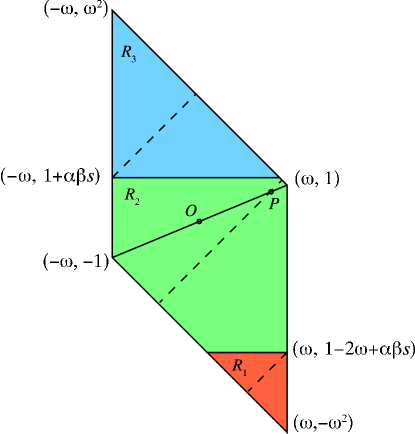
Figure 4: Partition of the rhombus $\mathrm{R}$ into atoms $R_{i},\;i=1,2,3$. The piecewise isometry $\rho(s)$ may be represented as a composition of two involutions: simultaneous reflection of the atoms about their respective symmetry axes (dashed lines), followed by reflection about the short diagonal of the rhombus (solid line). The intersection of these symmetry lines is a fixed point $P$, located $s$ to the left and $\beta s$ below the vertex $(\omega,1)$.

The piecewise isometry $\rho(s)$ is reversible, namely it can be written as the composition of two orientation-reversing involutions,

$$\rho(s)=\mathtt{G}\circ\mathtt{H}(s),\qquad\mathtt{G}^{2}=\mathtt{H}(s)^{2}={\bf 1},$$

where $\mathtt{H}(s)$ is the simultaneous reflection of the three atoms about their respective symmetry axes, and $\mathtt{G}$ is the reflection of the rhombus $\mathrm{R}$ about its short diagonal. Note that the fixed point $P$ is symmetric, namely it lies at the intersection of fixed lines of $\mathtt{G}$ and $\mathtt{H}$. Moreover, $\mathtt{H}=\mathtt{G}\circ\rho$, and either $\mathtt{G}$ or $\mathtt{H}$ serves as a time-reversal operator for the map $\rho$:

$$\mathtt{G}\circ\rho(s)\circ\mathtt{G}=\mathtt{H}\circ\rho(s)\circ\mathtt{H}=\rho(s)^{-1}.$$

Another useful symmetry relation follows from the invariance of the rhombus under $\mathtt{R}_{4}$ (rotation by $\pi$), which takes $(x,y)$ into $(-x,-y)$. One readily verifies that

$$\mathtt{R}_{4}\circ\rho(s)\circ\mathtt{R}_{4}=\rho(2\omega-s).$$

In studying the renormalizability of the family over $[0,2\omega]$, we are thus permitted to restrict ourselves to $s\in[0,\omega]$. For reasons which will soon become clear, we will mainly be focusing on the shorter interval,

$$I=[0,\alpha].$$ (10)

Equipped with the $s$-dependent piecewise isometry $\rho(s)$, the rhombus $\mathrm{R}$ becomes the span of a parametric dressed domain $\mathcal{R}(s)=(\mathrm{R},\mathbf{R}(s),\rho(s))$. To demonstrate the renormalizability of $\mathcal{R}(s)$, as defined in section 2, is the principal goal of this investigation. To do this, we concentrate on the atom $R_{1}(s)$, showing that it is a dressed subdomain of $\mathcal{R}(s)$ and moreover is an example of a two-parameter family of base triangles. The renormalizability of base triangles will then occupy our efforts for the remainder of the article.

3.1 The base triangle

We define a two-parameter parametric dressed domain, the base triangle. For parameters $l\in\mathbb{R}_{+}$ and $h\in[0,\alpha l]$, we define a prototype $\widehat{{\mathcal{B}}}(l,h)=(\widehat{\mathrm{B}},\widehat{\mathbf{B}},\rho)$ to represent its equivalence class with respect to $\mathfrak{G}$. The dressed domain induced on the atom $R_{1}(s)$ of $\mathcal{R}$ will be shown below to be congruent to $\widehat{{\mathcal{B}}}(1,s)$.

The tiling $\widehat{\mathbf{B}}$ is illustrated in figure 5. The defining data are presented in Table 1. For simplicity, we choose a frame of reference with the right-angle vertex of $\widehat{\mathrm{B}}$ at the origin and the remaining vertices at points of the negative $x$ and $y$ axes.

Table 1: Tiling table of the prototype base triangle $\widehat{{\mathcal{B}}}(l,h)$, for $0<h/l<\alpha$.

$$\begin{array}[]{|c|c|c|c|c|c|c|}\hline\cr\vrule\lx@intercol\hfil\mbox{Source Polygon}\hfil\lx@intercol\vrule\lx@intercol&\vrule\lx@intercol\hfil\mbox{Initial Placement}\hfil\lx@intercol\vrule\lx@intercol&\vrule\lx@intercol\hfil\mbox{Destination}\hfil\lx@intercol\vrule\lx@intercol\\ \hline\cr\mbox{Tile}&Q_{\#}&\mbox{Parameters}&{\tt R}_{\#}&\mbox{Translation}&\mbox{Tile}&{\tt R}_{\#}\\ \hline\cr\hline\cr\widehat{\mathrm{B}}&1&\alpha l+\beta h&7&(0,0)&\mbox{---}&\mbox{---}\\ \hline\cr\hline\cr\widehat{B}_{1}&1&\alpha\beta l-\beta h&2&(-\alpha l-h,-\alpha\beta l+\beta h)&\mathtt{U}_{1}\widehat{B}_{1}&2\\ \hline\cr\widehat{B}_{2}&7&2l-\alpha h&0&(-2l+\alpha h,-2h)&\mathtt{U}_{1}\widehat{B}_{2}&3\\ \hline\cr\widehat{B}_{3}&6&\alpha l-h,h&0&(-h,-h)&\mathtt{U}_{1}\widehat{B}_{3}&2\\ \hline\cr\widehat{B}_{4}&7&\alpha h&5&(-2l+\alpha h,0)&\mathtt{U}_{1}\widehat{B}_{4}&1\\ \hline\cr\widehat{B}_{5}&1&\beta h&7&(-2l,0)&\mathtt{U}_{1}\widehat{B}_{5}&0\\ \hline\cr\end{array}$$

In the table, the atoms of $\widehat{\mathbf{B}}$ and their span are listed by giving their respective orientations and translation vectors relative to a representative tile in the catalogue of Appendix A. For example, we learn from table 1 that

$$\widehat{B}_{1}=\mathtt{T}_{\mathbf{d}}\,\mathtt{R}_{2}\,Q_{1}(\alpha\beta l-\beta h),$$

where $\mathbf{d}=(-\alpha l-h,-\alpha\beta l+\beta h)$ is the location of the offset tile’s anchor point (local origin; see Appendix A). The isometry $\rho_{1}$ associated with atom $\widehat{B}_{1}$ is uniquely specified by the information listed in the last two columns. Because $\mathbf{d}$ lies on the symmetry line of the tile, it is taken into $\mathtt{U}_{1}(\mathbf{d})$ by $\rho_{1}$. More generally, if $n_{1}$ is the rotation index of the last column of the table, we calculate

$$\rho_{1}=T_{\mathtt{U}_{1}\mathbf{d}-\mathtt{R}_{n_{1}}\mathbf{d}}\,\mathtt{R}_{n_{1}}.$$

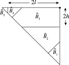
Figure 5: The prototype base triangle $\widehat{{\mathcal{B}}}(l,h)$ for $0<h/l<\alpha$.

The definition of the base triangle can be extended to the boundary of the parametric domain. This domain has two atoms for $h=0$ (and any $l$) and three for $h=\alpha l$; the atoms are still described by table 1 with the stipulation that all zero-parameter entries are to be deleted.

The following result establishes the dynamics of the base triangle, which is the basis of the renormalization process.

Proposition 1

For all $s\in I$, let $\mathcal{R}(s)=(\mathrm{R}(s),(R_{i}(s)),(\rho_{i}(s)))$ be the parametric dressed rhombus defined in equations (7)–(9). Then the atom $R_{1}(s)$, equipped with the return map induced by $\rho(s)$, is a dressed subdomain $\mathcal{B}$ congruent to the prototype base triangle $\widehat{\mathcal{B}}(1,s)$. The rhombus $\mathrm{R}(s)$ is tiled by the return orbits of the atoms of $\mathcal{B}$ and also of the periodic tiles

$$\begin{array}[]{l}\Pi_{1}=\mathtt{T}_{(-1-s,1-\beta s)}\,Q_{10}(s,\alpha-s),\\ \Pi_{2}=\mathtt{T}_{(-1-s,-\beta-\beta s)}\,Q_{5}(\alpha-s),\\ \Pi_{3}=\mathtt{T}_{(\omega-s,1-\beta s)}\,Q_{5}(s),\end{array}$$

apart from a set of zero measure. The incidence matrix for the return orbits of the atoms is:

$$\left(\begin{array}[]{ccccc}1&1&1&1&1\\ 8&5&2&4&6\\ 5&2&2&2&2\end{array}\right).$$

Proof. The proof is a straightforward application of the direct iteration method described in section 2.5. The initial and final tiles of the return orbits can be gleaned from table 1, and we know that the periodic orbits should begin and end on $\Pi_{k},\,k=1,2,3$. In the course of constructing the return orbits, we keep track of the atoms visited, obtaining at the end the symbolic paths and incidence matrices of the orbits. By adding up the areas of the tiles of all the orbits, and comparing with the total area of the parent domain, we prove the completeness of the tiling.

The details of the computer-assisted calculation may be found in the Electronic Supplement[6]. $\Box$

The tiling is illustrated for several values of $s$ in figure 6. The reader may find it instructive to follow each of the orbits around the rhombus, applying ‘by eye’ the product of local and global involutions at each step.

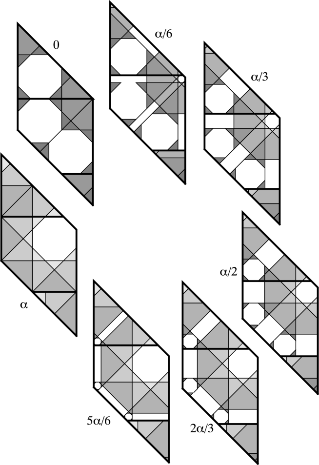
Figure 6: Tiling of the rhombus $\mathrm{R}$ by return orbits of the atoms of $R_{1}$ (shades of gray) and the periodic tiles $\Pi_{1},\Pi_{2},\Pi_{3}$ (white), for equally spaced values of $s=h/l$ in $I=[0,\alpha]$. The three atoms of $\mathcal{R}$ have been drawn with thicker boundaries.

4 Main results

We now state the main results of our investigation. We begin by defining the renormalization functions $f$ and $r=f^{2}$ (see figures 2 and 7), for all $s\in I=[0,\alpha]$:

$$f(0)=f(\alpha)=0,$$

$$f(s)=\omega^{|i|+1}\left\{\begin{array}[]{ll}(\Delta_{i}-s)&s\in I_{i},\;i<0\\ (s-\beta)&s\in I_{0}\\ (s-\Delta_{i})&s\in I_{i},\;i>0,\end{array}\right.$$ (11)

where

$$I_{i}=\left\{\begin{array}[]{ll}(\Delta_{i-1},\Delta_{i}]&i<0\\ (\beta,1)&i=0\\ \left[\Delta_{i},\Delta_{i+1})\right.&i>0\end{array}\right.\qquad\Delta_{i}=\left\{\begin{array}[]{ll}\beta^{|i|}&i<0\\ \beta,&i=0\\ \alpha-\beta^{|i|}&i>0\end{array}\right.$$ (12)

and

$$r(0)=r(\alpha)=0,$$

$$r(s)=\omega^{|i|+|j|+2}\left\{\begin{array}[]{ll}(\Delta_{i,j}-s)&s\in I_{i,j},\quad j<0\mbox{ or }(j=0\mbox{ and }i<0),\\ (s-\Delta_{i,j})&s\in I_{i,j},\quad j>0\mbox{ or }(j=0\mbox{ and }i\geq 0),\end{array}\right.$$ (13)

where

$$I_{i,j}=\left\{\begin{array}[]{ll}(\Delta_{i,j-1},\Delta_{i,j}]&j<0\\ (\Delta_{i,-1},\Delta_{i,0})&j=0,\,i<0\\ (\Delta_{i,0},\Delta_{i,1})&j=0,\,i\geqslant 0\\ \left[\Delta_{i,j},\Delta_{i,j+1})\right.&j>0,\end{array}\right.$$

$$\Delta_{i,j}=\left\{\begin{array}[]{ll}\beta^{|i|+1}+\beta^{|i|+|j|+1}&i\leqslant 0,\,j\leqslant 0\\ \beta^{|i|}-\beta^{|i|+|j|+1}&i<0,\,j>0\\ \alpha-\Delta_{-i,-j}&i>0\mbox{ or }(i=0\mbox{ and }j>0).\end{array}\right.$$

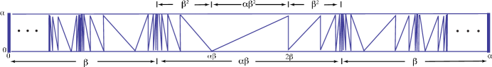
Figure 7: The piecewise-affine renormalization function $r=f^{2}$

.

The following two theorems constitute our main results.

Theorem 1

Let ${\mathcal{B}}$ be a parametric base triangle congruent to the prototype $\widehat{{\mathcal{B}}}(l,sl)$. Then ${\mathcal{B}}$ is renormalizable for all positive real $l$ and $s\in I$. Specifically:

$i)$ For $s\in\{0,\alpha\}$, ${\mathcal{B}}$ has a dressed subdomain ${\mathcal{B}}^{*}$ congruent to $\widehat{{\mathcal{B}}}(\kappa(s)l,0)$, with

$$\kappa(0)=\beta,\qquad\kappa(\alpha)=1.$$

The parity $\pi({\mathcal{B}}^{*})$ is $-\pi({\mathcal{B}})$ for $s=0$ and $\pi({\mathcal{B}})$ for $s=\alpha$. The return-map orbits of the atoms of ${\mathcal{B}}^{*}$, together with those of a finite number of periodic tiles, tile the spanning triangle of ${\mathcal{B}}$, up to a set of measure zero.

$ii)$ For all $i\in\mathbb{Z}\setminus\{0\}$ and $s=\Delta_{i}$, as defined in (12), the domain ${\mathcal{B}}$ has two dressed subdomains, ${\mathcal{B}}^{*}$ and ${\mathcal{B}}^{\dagger}$ congruent, respectively, to $\widehat{{\mathcal{B}}}(\kappa^{*}(\Delta_{i})l,0)$ and $\widehat{{\mathcal{B}}}(\kappa^{\dagger}(\Delta_{i})l,0)$, with

$$\kappa^{*}(\Delta_{i})=\beta^{|i|}/\alpha,\qquad\kappa^{\dagger}(\Delta_{i})=\beta^{|i|+2}/\alpha.$$

The parities $\pi({\mathcal{B}}^{*})$ and $\pi({\mathcal{B}}^{\dagger})$ are both $(-1)^{|i|+1}\pi({\mathcal{B}})$. The return-map orbits of the atoms of ${\mathcal{B}}^{*}$ and ${\mathcal{B}}^{\dagger}$, together with those of a finite number of periodic tiles, tile the spanning triangle of ${\mathcal{B}}$, up to a set of measure zero.

$iii)$ For all $i,j\in\mathbb{Z}$ and $s\in I_{i,j}$, the dressed domain ${\mathcal{B}}$ has a dressed subdomain ${\mathcal{B}}^{*}$ congruent to $\widehat{{\mathcal{B}}}(l^{*},s^{*}l^{*}),\;l^{*}=\kappa(s)l,\;s^{*}=r(s)$, with $r(s)$ given by (13) and

$$\kappa(s)=\beta^{|i|+|j|+2},\qquad\pi({\mathcal{B}}^{*})=(-1)^{|i|+|j|}\pi({\mathcal{B}}).$$

The return-map orbits of the atoms of ${\mathcal{B}}^{*}$, together with those of a finite number of periodic tiles, tile the spanning triangle of ${\mathcal{B}}$, up to a set of measure zero. The tilings vary continuously with respect to $s\in I_{i,j}$, with the return paths (hence the incidence matrix) constant over the interior of the interval.

There is a tight connection between strict renormalizability and the field $\mathbb{Q}(\sqrt{2})$, due to the following result.

Theorem 2

The renormalization function $f$ is conjugate to a left shift acting in a space of one-sided symbol sequences with alphabet $\mathbb{Z}\cup\{-\infty,+\infty\}$. A point $s\in I$ is eventually periodic under $f$ if and only if $s\in\mathbb{Q}(\sqrt{2})$. Hence the set of values of $s$ for which a base triangle congruent to $\widehat{{\mathcal{B}}}(l,sl)$ is strictly renormalizable is $\mathbb{Q}(\sqrt{2})\cap I$.

Theorem 1 will be proved from the analysis of the return-map dynamics. Before that rather lengthy analysis, we will prove theorem 2 and study some interesting properties of the function $f$ and its symbolic dynamics.

5 Symbolic dynamics

In this section we introduce a symbolic dynamics for $f$ which will give us a useful expansion for $s\in I$ —equation (21). This is a variant of the so-called Lüroth expansions [15, 8, 3].

The renormalization map $f$, see (11) and figure 2, is piecewise-affine, and its restriction to the interval $I_{i}$ has slope $\pm\omega^{|i|+1}$. Since $\omega>1$, this map is expanding, and since the length of $I_{i}^{\pm}$ is equal to $\alpha\beta^{|i|+1}=\alpha/\omega^{|i|+1}$, we see that $f(I_{i})=I$ (with the origin missing if $i=0$). It follows that $f$ preserves the Lebesgue measure.

Next we define the function $i:I\to\mathbb{Z}\cup\{-\infty,+\infty\}$ which assigns to each $s$ the interval $I_{i}$ to which it belongs. Explicitly,

$$i(s)=\left\{\begin{array}[]{ll}\lfloor\log_{\beta}(s)\rfloor&\qquad 0<s\leqslant\beta\\ \lfloor\log_{\beta}(\alpha-s)\rfloor&\qquad\beta<s<\alpha\\ -\infty&\qquad s=0\\ +\infty&\qquad s=\alpha.\end{array}\right.\\$$ (14)

In terms of this function, $f$ can be rewritten as

$$f(s)=\left\{\begin{array}[]{ll}\sigma(i(s))\,\omega^{|i(s)|+1}\,\bigl{(}s-\Delta_{i(s)})&\quad s\not=0,\alpha\\ 0&\quad s=0,\alpha,\end{array}\right.$$ (15)

where

$$\sigma(i)=\left\{\begin{array}[]{ll}-1&i<0\\ 1&i\geqslant 0.\end{array}\right.$$ (16)

Let us now consider the orbit of $f$ with initial condition $s_{0}=s\in I$. For all $k\geqslant 0$ we let $s_{k+1}=f(s_{k})$. With the notation

$$i_{k}=i(s_{k}),\qquad\sigma_{k}=\sigma(i_{k}),\qquad\pi_{k}=\alpha(1+\sigma_{k})/2,$$ (17)

equation (15) becomes

$$s_{k+1}=\left\{\begin{array}[]{ll}\sigma_{k}\omega^{|i_{k}|+1}\,(s_{k}-\pi_{k}+\sigma_{k}\beta^{|i_{k}|})&\quad s_{k}\not=0,\alpha\\ 0&\quad s_{k}=0,\alpha.\end{array}\right.$$ (18)

In this way, every $s\in I$ is associated with a unique sequence

$$(i_{0},i_{1},i_{2},\ldots\,)$$ (19)

with $i_{k}\in\mathbb{Z}\cup\{-\infty,+\infty\}$. The only constraints which we impose on these sequences is that the sub-strings $(\mp\infty,r),\;r\neq-\infty$ are forbidden, and that the symbol $+\infty$ can only appear as the leading symbol: $(+\infty,-\infty,\ldots)$. In the space of such sequences, a left shift is conjugate to the map $f$ on $I$.

To establish that each allowed sequence (19) corresponds to a unique $s$, we begin with the sequences $(\mp\infty,-\infty,-\infty,\ldots)$, which represents exclusively the value $0$ (negative sign) and $\alpha$ (positive sign). All other sequences either have no symbols $-\infty$, or else have an infinite tail of $-\infty$ symbols preceded by a finite sequence in which $\mp\infty$ does not appear. In either case, we can assume $s_{k}\neq 0,\alpha$ and invert (18) to obtain

$$s_{k}=\pi_{k}-\sigma_{k}\beta^{|i_{k}|}+\sigma_{k}\beta^{|i_{k}|+1}s_{k+1}.$$ (20)

Iterating, we find:

$$s_{0} = \pi_{0}-\sigma_{0}\beta^{|i_{0}|}+\sigma_{0}\beta^{|i_{0}|+1}s_{1}$$

$$= \pi_{0}-\sigma_{0}(\omega-\pi_{1})\beta^{|i_{0}|+1}-\sigma_{0}\sigma_{1}\beta^{|i_{0}|+|i_{1}|+1}+\sigma_{0}\sigma_{1}\beta^{|i_{0}|+|i_{1}|+2}s_{2}.$$

An easy induction gives

$$s=s_{0}=\pi_{0}-\Lambda\hskip 40.0pt\Lambda=\sum_{n\geqslant 1}a_{n}\beta^{n+b_{n}},$$ (21)

where

$$a_{n}=(\omega-\pi_{n})\prod_{k<n}\sigma_{k}\hskip 40.0ptb_{n}=\sum_{k<n}|i_{k}|.$$ (22)

The sequence $(b_{n})$ is non-negative and non-decreasing, and we have $b_{n}\equiv 0$ only for the fixed point $s=\sqrt{2}/2$. The sequence $(a_{n})$ depends only on the $\sigma_{k}$s; indeed,

$$\omega-\pi_{n}=\left\{\begin{array}[]{ll}\omega&\quad\sigma_{n}=-1\\ 1&\quad\sigma_{n}=+1.\end{array}\right.$$ (23)

Thus $a_{n}\in\{\pm 1,\pm\omega\}$.

The sum in (21) is absolutely convergent, and it provides an expansion for any $s\in[0,\alpha)$. On the other hand, having excluded $+\infty$ from all but one sequence, distinct sequences correspond to distinct values of $s\in[0,\alpha]$. This completes the proof of the claimed bi-unique correspondence.

The expansion (21) is finite if the orbit of $s_{0}$ reaches the origin, and infinite otherwise. In the former case $\Lambda$ is a finite sum of elements of $\mathbb{Z}[\alpha]$, and hence $s\in\mathbb{Z}[\alpha]$. If the sequence (19) is eventually periodic with limiting period $N$, then the sequence $a_{n}$ is eventually periodic with the same transient and period $N$ or $2N$, while the sequence $b_{n}$ eventually becomes the sum of an affine function plus a periodic function with period dividing $N$. Then the sum $\Lambda$ decomposes into the sum of finitely many geometric progressions, and so $\Lambda$, and hence $s$, belong to $\mathbb{Q}(\alpha)$.

In the next section we shall demonstrate that the converse is also true, namely that any $s\in\mathbb{Q}(\alpha)\cap[0,\alpha]$ has an eventually periodic symbol sequence of the type (19).

6 Lattice dynamics

Let the ring $\mathbb{Z}[\alpha]$ and the interval $I$ be given by (1) and (10), respectively. For $d\geqslant 1$, we define

$$\mathcal{M}_{d}=\frac{1}{d}\mathbb{Z}[\alpha]\cap I$$ (24)

which is the restriction to $I$ of the module $d^{-1}\mathbb{Z}[\alpha]$. Because $f(s)$ is obtained from $s$ by ring operations in $\mathbb{Z}[\alpha]$, and $f(I)=I$, we have that $f(\mathcal{M}_{d})\subset\mathcal{M}_{d}$. We have established the first part of the following lemma:

Lemma 1

For each $d$, we have

$$f(\mathcal{M}_{d})\subset\mathcal{M}_{d},\qquad f^{-1}(\mathcal{M}_{d}\setminus\{\alpha\})\subset\mathcal{M}_{d}.$$

Proof. It remains to show the invariance with respect to $f^{-1}$. In the statement of the lemma, the element $\alpha\in\mathcal{M}_{1}$ had to be removed since it is not in the domain of the function $f^{-1}$.

We have $0\in\mathcal{M}_{1}$, and, by construction we have

$$f^{-1}(\{0\})=\{\ldots,\Delta_{-2},\Delta_{1},\Delta_{0},\Delta_{1},\Delta_{2},\ldots\}\cup\{0,\alpha\}\subset\mathcal{M}_{1}.$$

Let now $s\not=0,\alpha$ and let $s^{\prime}=f(s)\in\mathcal{M}_{d}$. Using (11) we find

$$s=s^{\prime}\sigma(i(s))\beta^{|i(s)|+1}+\Delta_{i(s)}.$$

For any choice of the values of $i$, we see that $s$ is an affine function of $s^{\prime}$ with coefficients in $\mathbb{Z}[\alpha]$. Since $\mathbb{Z}[\alpha]/d$ is a module over $\mathbb{Z}[\alpha]$, it follows that $s\in\mathcal{M}_{d}$ (see (24)). $\Box$

Since, by the lemma, the inverse function cannot increase the denominator, then the forward function cannot decrease it. This can be rephrased as follows. For any $\xi\in\mathbb{Q}(\alpha)$, let $d^{*}=d^{*}(\xi)$ be the smallest natural number $d$ such that $\xi\in\mathcal{M}_{d}$. Then $d^{*}$ is a constant of the motion for the map $f$.

For $s\in\mathcal{M}_{d}$ we let $\zeta=sd$. Then $\zeta\in\mathbb{Z}[\alpha]\cap dI$, and alongside the interval map $s\mapsto f(s)$, we have the ring map

$$f_{d}:\mathbb{Z}[\alpha]\to\mathbb{Z}[\alpha]\qquad\zeta\mapsto\sigma(i(s))\omega^{|i(s)|+1}\left(\zeta-d\Delta_{i(s)}\right)\quad s=\frac{1}{d}\,\zeta$$ (25)

(with $f_{d}(0)=f_{d}(d\alpha)=0$) which represents the restriction of $f$ to $\mathcal{M}_{d}$ after clearing denominators.

Conclusion of the proof of theorem 2. We introduce the natural bijection

$$\phi:\mathbb{Z}[\alpha]\to\mathbb{Z}^{2}\qquad m+n\alpha\mapsto(m,n)$$

which conjugates $f_{d}$ to a lattice map on $\mathbb{Z}^{2}$, for which still use the same symbol.

For any $d>0$, we define the infinite strip

$$\Sigma_{d}=\left\{(m,n)\in\mathbb{Z}^{2}\,:\,-m\leqslant n\alpha\leqslant-m+d\alpha\right\},$$

which is invariant under $f_{d}$ (because $I$ is invariant under $f$).

We claim that all orbits of the map $f_{d}$ are eventually periodic. Since $\Sigma_{d}\subset\mathbb{Z}^{2}$ this means that all orbits of $f_{d}$ are bounded. Multiplication by $\omega$ in $\mathbb{Z}[\alpha]$ induces a linear map $M$ on $\mathbb{Z}^{2}$, with eigenvalues $-\omega,\beta$. The lines $\alpha y=\pm x$ are the corresponding eigendirections. Let $z\in\Sigma_{d}$, and let $(z_{-},z_{+})$ be the components of $z$ with respect to a basis of eigenvectors.

Since the expanding eigendirection is transversal to $\Sigma_{d}$, there is a constant $c_{d}$ such that $|z_{+}|<c_{d}$. So it suffices to show that the component $z_{-}$ remains bounded. For all $z\in\mathbb{Z}^{2}$ and $i\geqslant 0$ we have

$$|M^{j+1}(z)_{-}|\leqslant\beta|z_{-}|<|z_{-}|.$$ (26)

Furthermore, from (12) we have that $\omega^{|i|+1}\Delta_{i}$ is a monomial or binomial in $\omega$ of degree at most ${|i|+1}$ with coefficients $1,-1,\alpha$. Defining

$$C=d\,(|\phi(1)_{-}|+|\phi(-1)_{-}|+|\phi(\alpha)_{-}|)$$

from (26) we have

$$|M^{|i|+1}(\phi(d\Delta_{i}))_{-}|\leqslant|\phi(d\Delta_{i})_{-}|\leqslant C.$$ (27)

Finally, from (25), (26), and (27), we obtain

$$|f_{d}(z)_{-}|\leqslant\beta|z_{-}|+C$$

and since $\beta<1$, for all sufficiently large $|z_{-}|$ the map $f_{d}$ is a contraction mapping. Thus its orbits are bounded hence eventually periodic.

This completes the proof of theorem 2. $\Box$

7 Overview of the renormalization dynamics

As a prelude to the proof of theorem 1, we now turn our attention to the dynamical underpinnings of the renormalizability of the parametric base triangle ${\mathcal{B}}(l,s)$. This analysis is based on the construction of the return-map tree through successive inductions on sub-domains, a process which is far more complex than one might guess from the simple functional form of the function $r$. To account for the renormalizability of the entire parameter interval, ten distinct renormalization scenarios need to be considered, each characterized by the participation of distinctive parametric dressed domains. We have given such special domains names suggestive of their geometric structure: the pencil ${\mathcal{P}}$, the fringed triangle ${\mathcal{T}}$, and the double strip ${\mathcal{D}}$. The induction sequence for each of the ten scenarios and the corresponding parameter intervals are specified in Table 2. In the labelling of the scenarios, Roman numerals I through IV are used to indicate the major classifications, with asterisks and binary subscripts $\mu,\nu=\pm 1$ indicating finer distinctions (to be clarified in the next section).

Table 2: Renormalization scenarios, each one corresponding to a simple closed loop on the renormalization graph of figure 8. (See also figures 9 and 10.)

$$\begin{array}[]{|c|c|c|}\hline\cr\vrule\lx@intercol\hfil\mbox{Renormalization scenario}\hfil\lx@intercol\vrule\lx@intercol&\mbox{Ranges of indices}\\ \hline\cr\mbox{I}&{{\mathcal{B}}}\rightarrow{{\mathcal{B}}}&\begin{array}[]{c}(\pm\infty,0),\,(0,\pm\infty)\\ (-1,j),\;(1,-j),\quad j=0,1,2,3\\ (0,j),\quad|j|\leqslant 2.\end{array}\\ \hline\cr\mbox{II}&{{\mathcal{B}}}\rightarrow{\mathcal{P}}\rightarrow{\mathcal{P}}^{*}\rightarrow{{\mathcal{B}}}&\begin{array}[]{c}(i,j),(-i,-j),\;\;i\geqslant 2,\;\;-3\leqslant j\leqslant 2,\\ (1,j),\;(-1,-j),\quad j=1,2,\\ (-i,-\infty),\,(i,+\infty),\quad i\geqslant 1.\end{array}\\ \hline\cr\mbox{III}_{\mu\nu}&{{\mathcal{B}}}\rightarrow{\mathcal{T}}_{\mu}\rightarrow{\mathcal{D}}_{\mu}\rightarrow{\mathcal{D}}^{*}_{\nu}\rightarrow{{\mathcal{B}}}&\begin{array}[]{l}\mu=-1:\quad(0,\pm j),\quad j\geqslant 3,\\ \mu=+1:\quad(1,-j),\;(-1,j),\quad j\geqslant 4,\\ \nu=(-1)^{j}.\end{array}\\ \hline\cr\mbox{IV}_{\mu\nu}&{{\mathcal{B}}}\rightarrow{\mathcal{P}}\rightarrow{\mathcal{T}}_{\mu}\rightarrow{\mathcal{D}}_{\mu}\rightarrow{\mathcal{D}}^{*}_{\nu}\rightarrow{{\mathcal{B}}}&\begin{array}[]{l}\mu=-1:\quad(i,j),\;(-i,-j),\;i\geqslant 1,\;\;j\geqslant 3,\\ \mu=+1:\quad(-i,j),\;(i,-j),\;i\geqslant 2,\;\;j\geqslant 4,\\ \nu=(-1)^{j}.\end{array}\\ \hline\cr\end{array}$$

The rest of this section is devoted to graphical representations of the ten scenarios, the most important of which is the renormalization graph of figure 8. Each vertex of the graph corresponds to an equivalence class of parametric dressed domains. Thus the vertex ${\mathcal{B}}$ represents a base triangle congruent to the prototype $\widehat{{\mathcal{B}}}(l,h)$, with $l>0$ and $s=h/l\in I$. The precise interpretation of the remaining vertices will emerge from the prototype definitions and lemmas of section 8, together with the specification of parameter ranges in the propositions of section 10. An oriented edge of the graph, $\mathcal{X}\rightarrow\mathcal{Y}$, signifies that ${\cal Y}$ is a dressed sub-domain of ${\cal X}$, which is dressed by $\mathcal{X}$ via induction. Each edge is labelled by subscripted Roman numerals, indicating the relevant parameter constraints listed in Table 2. Loops in the graph correspond to renormalization scenarios and since $\mu,\nu=\pm 1$, there are ten different scenarios in all.

In labelling the vertices of the graph, we have used asterisks to differentiate members of the same family. For example, ${\mathcal{P}}$ and ${\mathcal{P}}^{*}$ are both pencils, the latter being minimal in a sense to be made clear in section 8.2. If ${\mathcal{P}}$ is already minimal, then ${\mathcal{P}}$ coincides with ${\mathcal{P}}^{*}$ and the edge simply represents the identity.

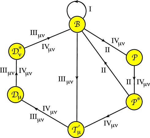
Figure 8: Renormalization graph, whose closed loops are the renormalization scenarios of Table 2.

Figure 9 emphasizes the organisation of the ten scenarios on the $s$-axis. Specifically, we display the sub-intervals $I_{i,j}$ and their assignment to the scenarios I–IV for $\beta^{4}\leqslant s\leqslant 1$. The same information is illustrated in figure 10 on the $(i,j)$-lattice. Here the labels I–IV denote subsets of $\mathbb{Z}^{2}$, with suitable added points at infinity. We see that scenario I is restricted to pairs $(i,j)$ where both indices are small, plus four points at infinity corresponding to $s=\alpha,0$ and $s=\beta,1$, respectively. Scenario II corresponds to small values of $j$, with unbounded $i$ (corresponding to $s$ approaching $0,\alpha$), plus a sequence of points at infinity corresponding to the accumulation points $\beta^{|i|+1}$ and $\alpha-\beta^{|i|+1}$, for $|i|\geqslant 1$. Scenario III features small values of $i$ and unbounded $j$ (corresponding to $s$ tending to an accumulation point). Finally, scenario IV covers the doubly asymptotic cases. With reference to table 2, we shall use the short-hand notation:

$$\mathrm{III}=\bigcup_{\mu,\nu}\mathrm{III}_{\mu\nu}\hskip 30.0pt\mathrm{IV}=\bigcup_{\mu,\nu}\mathrm{IV}_{\mu\nu}.$$ (28)

Our classification scheme leaves open the possibility of more than one realization of each scenario. Thus, even though mirror sub-intervals $I_{i,j}$ and $I_{-i,-j}$ always belong to the same scenario (as evident in the symmetry of Table 2), the difference in their return paths may be sufficient to have distinct temporal scaling properties. This essentially doubles the number of incidence matrices which we need to calculate.

The dynamical architecture of renormalization in the present model bears a strong, if imperfect, resemblance to that of Rauzy [19, 22] to construct renormalizable interval exchange transformations (IETs), i.e., maps on an interval $I$ which permute $n$ sub-intervals which form a partition of $I$. At the heart of the Rauzy construction is an irreducible graph (Rauzy graph), each vertex of which is a ‘parametric IET’ corresponding to a permutation of $n$ symbols and parametrized by a positive $n$-vector $\mathbf{s}$ of interval lengths. The IET’s of the graph are known as a Rauzy class. Each vertex has two outgoing edges, corresponding to two possible induced return maps, and is associated with a matrix transformation in parameter space, $\mathbf{s}\mapsto\mathbf{r}_{i}\cdot\mathbf{s},\;i=0,1$. To search for strictly renormalizable IET’s, one considers the closed loops of the Rauzy graph, multiplying the $\mathbf{r}_{i}$ matrices around a loop and seeking a positive eigenvector of the product matrix.

In the present work, our strategy for proving renormalizability is clearly analogous to Rauzy’s, but of course there are important differences. In particular, our ‘Rauzy class’ of base triangles, pencils, fringed triangles, and double strips is a more variegated collection of parametric dressed domains, with bifurcating parameter dependence and no uniform rules of induction to compare with Rauzy’s. Nevertheless, the general strategy (also applied in the context of polygon-exchange transformations by Schwartz [21]) is the same.

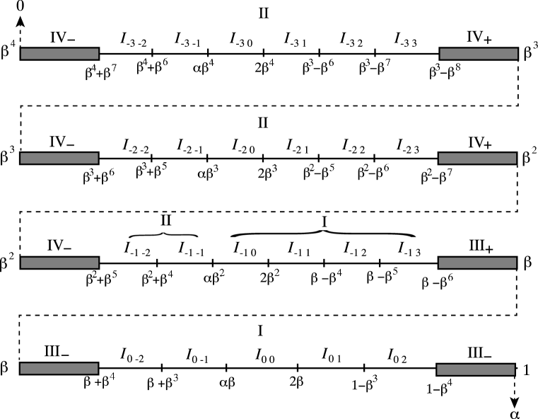
Figure 9: Portion of the $s$-axis, folded, with distorted scale. The large-$|j|$ asymptotic regime (scenarios III and IV) is represented by thick segments surrounding the accumulation points $\beta^{k},\;k=1,2,3,4$. The large-$|i|$ regime (scenarios II and IV) consists of the entire interval $[0,\alpha\beta^{2}]$.

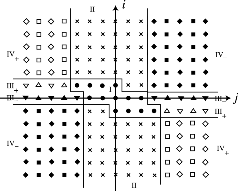
Figure 10: The ten renormalization scenarios for the indices $(i,j)\in\mathbb{Z}^{2}$. We write $\pm$ for $\pm 1$. The labels ${\rm III}_{\pm}$ and ${\rm IV}_{\pm}$ stand for ${\rm III}_{\pm-}\cup{\rm III}_{\pm+}$ and ${\rm IV}_{\pm-}\cup{\rm IV}_{\pm+}$, respectively. Key: ${\rm I}=\bullet,\;{\rm II}=\times,{\rm III}_{++}=\vartriangle,\;{\rm III}_{+-}=\triangledown,\;{\rm III}_{-+}=\blacktriangle,\;{\rm III}_{--}=\blacktriangledown,{\rm IV}_{++}=\square,\;{\rm IV}_{+-}=\diamondsuit,\;{\rm IV}_{-+}=\blacksquare,\;{\rm IV}_{--}=\blacklozenge.$

8 Parametric dressed domains with strips

The reader has already been alerted to the fact that certain classes of parametric dressed domains (pencils, fringed triangles, and double strips) play central roles in our renormalization story. We now define these objects. A common feature of all of them is the presence of a special, quasi-one-dimensional sub-tiling which we call the strip.

8.1 The strip

The prototype strip $\widehat{\bf S}(l,h)$ is a tiling with a variable number

$$2J=2\lfloor\log_{\beta}(h/l)\rfloor$$ (29)

of tiles, all of which are reflection-symmetric. If we let $h$ tend monotonically to zero, the strip undergoes a bifurcation every time $h/l$ assumes a value $\beta^{k},\;k=2,3,\ldots$. The number of tiles increases by two, with the additional tiles being born at one of the vertices at $x=-h$. The precise structure of $\widehat{\bf S}(l,h)$ is specified in table 3, and illustrated, for $J=4$, in figure 11.

Figure 11: A strip with 8 tiles.

Table 3: Tiling table of the prototype strip $\widehat{\bf{S}}(l,h)$. The origin of coordinates lies on the mid-line of the strip, at distance $h$ to the right of its vertical edge.

$$\begin{array}[]{|c|c|c|c|c|}\hline\cr\vrule\lx@intercol\hfil\mbox{Source Polygon}\hfil\lx@intercol\vrule\lx@intercol&\vrule\lx@intercol\hfil\mbox{Placement}\hfil\lx@intercol\vrule\lx@intercol\\ \hline\cr\mbox{Tile}&Q_{\#}&\mbox{Parameters}&{\tt R}_{\#}&\mbox{Translation}\\ \hline\cr\hline\cr\widehat{\rm S}&12&\alpha(l-h),2h&0&(-\alpha l+\beta h,-h)\\ \hline\cr\hline\cr\widehat{S}_{1}&4&\beta l-\beta h,\beta l-\omega h&0&(-l,0)\\ \hline\cr\widehat{S}_{2}&3&h&7&(-\alpha\beta l,0)\\ \hline\cr\begin{array}[]{c}\widehat{S}_{2j-1}\\ {}_{2\leqslant j\leqslant J-2}\end{array}&4&\beta^{j}l-\beta h,\beta^{j}l-\omega h&\begin{array}[]{cc}4&j\mbox{ even}\\ 0&j\mbox{ odd}\end{array}&(-\beta^{j-1}l,(-1)^{j-1}(\beta^{j}l-\alpha h))\\ \hline\cr\begin{array}[]{c}\widehat{S}_{2j}\\ {}_{2\leqslant j\leqslant J-2}\end{array}&3&h&\begin{array}[]{cc}0&j\mbox{ even}\\ 7&j\mbox{ odd}\end{array}&(-\alpha\beta^{j}l,0)\\ \hline\cr\widehat{S}_{2J-3}&1&\beta^{J-1}l-\beta h&\begin{array}[]{cc}0&J\mbox{ even}\\ 4&J\mbox{ odd}\end{array}&(-\beta^{J-2}l,(-1)^{J}(\beta^{J-1}l-\alpha h))\\ \hline\cr\widehat{S}_{2J-2}&8&-\alpha\beta^{J-1}l+\alpha\beta h,2h&\begin{array}[]{cc}1&J\mbox{ even}\\ 6&J\mbox{ odd}\end{array}&(-\alpha\beta^{J-1}l-\beta h,(-1)^{J-1}h)\\ \hline\cr\widehat{S}_{2J-1}&1&\beta^{J}l-\beta h&\begin{array}[]{cc}4&J\mbox{ even}\\ 0&J\mbox{ odd}\end{array}&(-\beta^{J-1}l,(-1)^{J-1}(\beta^{J}l-\alpha h))\\ \hline\cr\widehat{S}_{2J}&7&\alpha\beta^{J-1}l-\alpha h&\begin{array}[]{cc}3&J\mbox{ even}\\ 6&J\mbox{ odd}\end{array}&(-h,(-1)^{J-1}(\alpha\beta^{J-1}l-\omega h)))\\ \hline\cr\end{array}$$

8.2 The pencil

The prototype pencil $\widehat{{\mathcal{P}}}(l,h)$ is a parametric dressed pentagon with a variable number

$$2L+1=4+\lfloor\log_{\beta}(\frac{h}{l})\rfloor$$

of atoms. Its tiling $\widehat{\mathbf{P}}$ is the union of five individual tiles and a strip, namely

$$\widehat{\bf P}=P_{0}\cup P_{1}\cup P_{2}\cup P_{3}\cup P_{4}\cup{\tt U}_{0}\widehat{\bf S}(\beta l,h),$$

Here we assume a coordinate system aligned with the axis of the pencil and with origin at the centre of the square tile $\widehat{P}_{0}$. Explicitly, arranging the tiles, apart from $\widehat{P}_{0}$, in left-to-right order of their anchor points, we have

$$\widehat{P}_{0} = Q_{2}(h)$$

$$\widehat{P}_{1} = {\tt T}_{(-l,0)}\,Q_{9}(\beta l/\alpha-h,h),$$

$$\widehat{P}_{2} = {\tt T}_{(-\alpha\beta l-\omega h,-h)}\,{\tt R}_{1}\,Q_{7}(\alpha h),$$

$$\widehat{P}_{3} = {\tt T}_{(-\alpha\beta l-h,-h)}\,{\tt R}_{3}\,Q_{1}(\beta h),$$

$$\widehat{P}_{4} = {\tt T}_{(-\alpha\beta l,0)}\,{\tt R}_{7}\,Q_{3}(h),$$

$$\widehat{P}_{k+4} = {\tt U}_{0}\,S_{k}(\beta l,h),\;k=1,\ldots,2L-4.$$

The span of the tiling is

$$\widehat{\rm P}={\rm span}(\widehat{\bf P})={\tt T}_{(-\alpha l+\alpha h,0)}\,Q_{6}(\alpha l-\omega h,h).$$

The structure of the pencil is illustrated in fig. 12.

Figure 12: The pencil prototype $\widehat{{\mathcal{P}}}(l,h)$ with $2L+1$ atoms, for $L=6$, together with the two sub-pencils ($L=5$ and $L=4$) obtained by application of the Pencil Shortening Lemma. Each shortening step (i) contracts the parameter $l$ by a factor $\beta$, with no change in the parameter $h$, (ii) reduces the number of atoms by two, and (iii) reverses the parity. The nine-atom pencil at the bottom cannot be shortened further without violating the definition of a pencil.

The domain map $\rho_{\stackrel{{\scriptstyle}}{{\widehat{{\mathcal{P}}}}}}$ for the pencil is defined in terms of a composition of involutions, ${\tt U}_{0}\circ{\tt H}$, where ${\tt H}$ is a simultaneous reflection of each tile about an assigned axis. The trapezia, triangles, kites, and the hexagon $\widehat{P}_{2L-2}$ have a unique reflection symmetry. For the rhombi, we choose the short diagonal, as in the case of the strip. This leaves the square $\widehat{P}_{0}$ and hexagon $\widehat{P}_{1}$, for which we assign axes parallel to $\mathbf{u}_{7}$ and $\mathbf{u}_{2}$, respectively.

Studying the renormalization of pencils with arbitrarily many atoms is made manageable by the Pencil Shortening Lemma, which relates any pencil to a minimal one with only nine atoms. Note that in specifying the associated incidence matrix, we use as matrix indices the canonical atom labels shown in figure 11. For the sake of transparency, we will adopt this convention for all of our incidence matrices throughout this article.

Pencil Shortening Lemma. Let ${\mathcal{P}}(l,h)=(\mathrm{P}(l,h),{\bf P}(l,h),\rho(l,h))$ be a pencil congruent to $\widehat{{\mathcal{P}}}(l,h)$, with $2L+1$ tiles (cf. equation (5)). The return maps induced by $\rho(l,h)$ on the tiles ${\rm P}(\beta^{k}l,h),\;k=1,\ldots,L-4,$ promote the latter to pencils of parity $(-1)^{k}$ congruent to $\widehat{P}(\beta^{k}l,h)$. For a given $L$, the minimal pencil induced by this shortening process has nine atoms, parity $(-1)^{L}$, and an incidence matrix (with respect to ${\mathcal{P}}(l,h)$) given, for $i=0,\ldots,2L+1$, by (we label the rows and columns of $\mathrm{M}$ by the canonical tile names ${\mathcal{P}}$ and ${\mathcal{P}}^{*}$, respectively)

$${\rm M}_{P_{i},P^{*}_{0}} = \delta_{i,0},$$

$${\rm M}_{P_{i},P^{*}_{1}} = \delta_{i,2L-5},$$

$${\rm M}_{P_{i},P^{*}_{2}} = \delta_{i,2}+2\sum_{j=4}^{2L-5}\delta_{i,j},$$ (30)

$${\rm M}_{P_{i},P^{*}_{3}} = 2(\delta_{i,2L-6}+\delta_{i,2L-5}),$$

$${\rm M}_{P_{i},P^{*}_{j}} = \delta_{i,j+2L-8},\;4\leqslant j\leqslant 8.$$

The polygon $\mathrm{P}(l,h)$ is tiled, up to a set of zero measure, by the return orbits of the tiles of the minimal pencil, as well as a finite number of periodic tiles.

Proof. Without loss of generality we assume ${\mathcal{P}}(l,h)=\widehat{{\mathcal{P}}}(l,h)$. We wish to show that the piecewise isometries $\rho^{(k)}$ of the shortened pencils ${\mathcal{P}}^{(k)}={\tt U}_{0}^{k}{\mathcal{P}}(\beta^{k}l,h)$ are induced return maps of $\rho^{(0)}=\rho(l,h)$. It suffices to prove it for $k=1$, since the step can be repeated until the pencil is minimal. The proof is by direct iteration of $\rho^{(0)}$ on the tiles of ${\mathcal{P}}^{(1)}$. Only a small number of tiles have non-trivial return orbits. To see this, we refer to figure 12. All of the tiles in the strip ${\bf S}(\beta^{2}l,h)$ are mapped the same by $\rho^{(0)}$ and by $\rho^{(1)}$. The same is true of $P^{(1)}_{0}$ and $P^{(1)}_{4}$, and even $P^{(1)}_{1}$. The remaining tiles, $P^{(1)}_{2}$ and $P^{(1)}_{3}$, have short return orbits which we calculate explicitly: we find that they pass through, in order, $P_{5},P_{4},P_{4},P_{5}$ and $P_{5},P_{4},P_{2},P_{4},P_{5}$, respectively.

From the structure of the return orbits, we can write down immediately the incidence matrix for the recursive step from $L$ to $L-1$. We label the rows and columns of the incidence matrix by the canonical tile names of $\mathrm{P}$:

$${\rm M}_{P^{(0)}_{i},P^{(1)}_{0}} = \delta_{i,0},$$

$${\rm M}_{P^{(0)}_{i},P^{(1)}_{1}} = \delta_{i,5},$$

$${\rm M}_{P^{(0)}_{i},P^{(1)}_{2}} = \delta_{i,2}+2(\delta_{i,4}+\delta_{i,5})$$ (31)

$${\rm M}_{P^{(0)}_{i},P^{(1)}_{3}} = 2(\delta_{i,4}+\delta_{i,5}),$$

$${\rm M}_{P^{(0)}_{i},P^{(1)}_{j}} = \delta_{i,j},\quad 6\leqslant i\leqslant 2L,\quad 4\leqslant j\leqslant 2L-2,$$

where in the first four equations the index $i$ varies over its full range: $0\leqslant i\leqslant 2L$.

For the full shortening process of $L-4$ steps, ending with a minimal pencil, the proof is by mathematical induction on $L$. The starting point is the case $L=5$, where the one-step incidence matrix is given by (31), which coincides with (30). Given formula (30) for a given $L$, we get the incidence matrix for $L+1$ by multiplication on the right by the recursion matrix defined by (31). One readily verifies that this reproduces the general formulae with $L$ incremented by one.

To prove the completeness of the tiling, it is again sufficient to restrict ourselves to a single shortening step. The periodic cells are readily identified cells: the hexagonal period-1 atom $P_{1}$, the triangular period-3 atom $P_{3}$, and an octagonal period-1 tile inscribed in the rhombic atom $P_{4}$. We explicitly verify that the total area of all return orbits is equal to that of the original pencil. That the minimal pencil has 9 atoms follows from the definition of a pencil, while the parity of $(-1)^{L}$ is a consequence of the fact that each of the $L-4$ shortening steps is accompanied by a reflection ${\tt U}_{0}$. $\Box$

8.3 Fringed triangle

There are two prototype fringed triangles $\widehat{\mathcal{T}}_{\pm}(l,h)$, each containing a strip congruent to $\widehat{\bf S}(l,h)$ with a variable number $2J$ of atoms. The total numbers of atoms are $2J+2$ for $\widehat{{\mathcal{T}}}_{-}(l,h)$ and $2J+7$ for $\widehat{{\mathcal{T}}}_{-}(l,h)$.

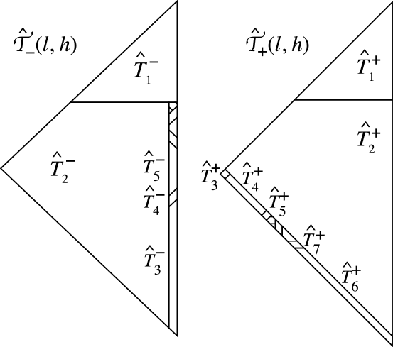
Figure 13: Tiling of the prototypes $\widehat{{\mathcal{T}}}_{\pm}(l,h)$.

We begin with $\widehat{{\mathcal{T}}}_{-}(l,h)$. Its tiling $\widehat{\bf T}_{-}$ is a union of two individual tiles with a strip, namely (see figure 13)

$$\widehat{\bf T}_{-}=\widehat{T}^{-}_{1}\cup\widehat{T}^{-}_{2}\cup{\tt R}_{2}\,{\bf S}(l,h).$$

Here we assume a coordinate system whose origin coincides with that of the strip, with the mid-line of the strip lined up along the negative $y$-axis. Explicitly,

$$\widehat{T}^{-}_{1} = {\tt T}_{(h,-h)}\,{\tt R}_{5}\,Q_{1}(\beta l+\beta h),$$

$$\widehat{T}^{-}_{2} = {\tt T}_{(-h,-\alpha l+\omega h)}\,{\tt R}_{3}\,Q_{7}(\alpha l-\alpha\omega h),$$

$$\widehat{T}^{-}_{k+2} = {\tt R}_{2}\,S_{k}(l,h),\;k=1,\ldots,2J.$$

The span of the tiling is

$$\widehat{\rm T}_{-}={\rm span}(\widehat{\bf T}_{-})={\tt T}_{(-l+\alpha h,-\beta l)}\,{\tt R}_{2}\,Q_{1}(l-\beta h).$$

Next we turn to the prototype fringed triangle $\widehat{{\mathcal{T}}}_{+}(l,h)$. Its tiling is the union of seven individual tiles and a strip, namely (see figure 13)

$$\widehat{\bf T}_{+}=\bigcup_{k=1}^{7}\widehat{T}^{+}_{k}\cup{\tt R}_{3}\,\widehat{\bf S}(l,h).$$

Here we assume a coordinate system whose origin coincides with that of the strip, with the mid-line of the strip lined up along the negative $y$-axis. Explicitly,

$$\widehat{T}^{+}_{1} = {\tt T}_{((3+\alpha)l-h,(1+2\alpha)l+h))}\,{\tt R}_{5}\,Q_{1}(\omega l-\beta h),$$

$$\widehat{T}^{+}_{2} = {\tt T}_{((3+\alpha)l-h,-(3+\alpha)l+\omega h)}\,{\tt R}_{3}\,Q_{7}(\alpha\omega^{2}l-\alpha h),$$

$$\widehat{T}^{+}_{3} = {\tt T}_{(-\alpha l,\alpha l)}\,{\tt R}_{7}\,Q_{2}(h),$$

$$\widehat{T}^{+}_{4} = {\tt T}_{(-l/\alpha,l/\alpha)}\,{\tt R}_{7}\,Q_{10}(h,l-h),$$

$$\widehat{T}^{+}_{5} = {\tt R}_{7}\,Q_{2}(h),$$

$$\widehat{T}^{+}_{6} = {\tt T}_{((3+\alpha)l-h,-l-h)}\,{\tt R}_{7}\,Q_{4}(\omega l-\beta h,\omega l-\omega h),$$

$$\widehat{T}^{+}_{7} = {\tt T}_{(l,-l)}\,{\tt R}_{7}\,Q_{3}(h),$$

$$\widehat{T}^{+}_{k+7} = {\tt R}_{3}\,S_{k}(l,h),\;k=1,\ldots,2J.$$

The span of the tiling is

$$\widehat{\rm T}_{+}={\rm span}(\widehat{\bf T}_{+})={\tt T}_{(-\alpha l+\alpha h,\alpha l)}\,{\tt R}_{2}\,Q_{1}(\omega^{2}l+\beta h).$$

The domain maps $\rho_{\stackrel{{\scriptstyle}}{{{\mathcal{T}}_{\pm}}}}$ of the fringed triangles are defined in terms of a composition of involutions, namely a simultaneous reflection of each atom about an assigned axis, followed by a reflection about the triangle’s symmetry axis. As in the case of the pencil, the assigned axis of each rhombic atom is its short diagonal. For the atoms $\widehat{T}^{+}_{3}$, $\widehat{T}^{+}_{4}$, and $\widehat{T}^{+}_{5}$, the assigned axes are parallel to $\mathbf{u}_{2},\mathbf{u}_{3}$, and $\mathbf{u}_{2}$, respectively.

8.4 Double strip

The prototype double strip $\widehat{{\mathcal{D}}}_{\nu}(l,h),\;\nu=\pm 1,$ is a dressed domain constructed out of a square and two strips, one on the left with positive parity and $2K$ atoms, the other on the right with negative parity and $2K-2$ atoms. Since a well-defined strip has at least four tiles, a double strip requires at least 11 atoms (i.e., $K\geqslant 3$). For both signs $\nu$, we define the prototype to have the tiling

$$\widehat{\bf D}(l,h)={\bf S}(\omega l,h)\,\cup\,\widehat{D}_{0}\,\cup{\tt U}_{2}\,{\bf S}(l,h),\hskip 30.0pt\widehat{D}_{0}=Q_{2}(h).$$

Note the appearance of the reflection operator ${\tt U}_{2}$ to correctly place and orient one of the component strips. A prototype double strip is illustrated in figure 14. Here and in what follows we adopt a canonical labelling of the tiles of any double strip ${\mathcal{D}}$, in order along the midline,

$$D^{{}^{\prime\prime}}_{1},D^{{}^{\prime\prime}}_{2},\ldots,D^{{}^{\prime\prime}}_{2K},D_{0},D^{{}^{\prime}}_{2K-2},\ldots,D^{{}^{\prime}}_{1},$$

Figure 14: Prototype double strip.

The distinction between $\widehat{{\mathcal{D}}}_{+}(l,h)$ and $\widehat{{\mathcal{D}}}_{-}(l,h)$ enters when we specify the piecewise isometry $\rho_{\stackrel{{\scriptstyle}}{{\widehat{{\mathcal{D}}}_{\nu}}}}$. As before, we define the map as a composition of two involutions, the reflection of each atom about an assigned symmetry axis, followed by reflection about the vertical symmetry axis of the double strip as a whole. Once again the axes of the rhombi are their short diagonals. The square $\widehat{D}_{0}$, on the other hand, is assigned the diagonal $\mathbf{u}_{1}$ for $\nu=+$ and $\mathbf{u}_{3}$ for $\nu=-$. A considerable simplification of the renormalization structure results from the following ‘shortening’ lemma:

Double-Strip Shortening Lemma. Let ${\mathcal{D}}(l,h)=(\mathrm{D}(l,h),{\bf D}(l,h),\rho(l,h))$ be a double strip congruent to $\widehat{{\mathcal{D}}}_{\nu}(l,h)$, with $4K-1$ tiles. The return maps induced by $\rho(l,h)$ on the tiles ${\tt U}_{2}^{k}{\rm D}(\beta^{k}l,h),\;k=1,\ldots,K-3,$ promote the latter to double strips of parity $(-1)^{k}$ congruent to $\widehat{D}_{\nu^{(k)}}(\beta^{k}l,h)$, with $\nu^{(k)}=(-1)^{k}\nu$. For a given $K$, the minimal double strip induced by this shortening process has 11 atoms, parity $(-1)^{K-3}$, index $\nu_{K-3}=(-1)^{K-3}\nu$, and an incidence matrix (with respect to ${\mathcal{D}}(l,h)$) given, for $K$ odd, by

$${\rm M}^{\rm odd}_{D,D_{0}} = \delta_{D,D_{0}}+{\rm N}_{D}^{\rm odd},$$

$${\rm M}^{\rm odd}_{D,D^{{}^{\prime\prime}}_{k}} = \delta_{D,D^{{}^{\prime\prime}}_{2K+k-6}}+{\rm N}_{D}^{\rm odd},\quad k=1,\ldots,6,$$ (32)

$${\rm M}^{\rm odd}_{D,D^{{}^{\prime}}_{k}} = \delta_{D,D^{{}^{\prime}}_{2K+k-6}}+{\rm N}_{D}^{\rm odd},\quad k=1\ldots,4,$$

$${\rm N}_{D}^{\rm odd}=\sum_{k=1}^{\frac{K-3}{2}}\left(2\cdot 4^{k-1}\,\delta_{D,D^{{}^{\prime\prime}}_{2K-4k-5}}+4^{k-1}\,\delta_{D,D^{{}^{\prime}}_{2K-4k-5}}\right),$$ (33)

and, for $K$ even, by

$${\rm M}^{\rm even}_{D,D_{0}} = \delta_{D,D_{0}}+{\rm N}_{D}^{\rm even},$$

$${\rm M}^{\rm even}_{D,D^{{}^{\prime\prime}}_{k}} = \delta_{D,D^{{}^{\prime}}_{2K+k-8}}+{\rm N}_{D}^{\rm even},\quad k=1,\ldots,6,$$ (34)

$${\rm M}^{\rm even}_{D,D^{{}^{\prime}}_{k}} = \delta_{D,D^{{}^{\prime\prime}}_{2K+k-4}}+{\rm N}_{D}^{\rm even},\quad k=1,\ldots,4,$$

$${\rm N}_{D}^{\rm even}=\sum_{k=1}^{\frac{K-2}{2}}\left(2\cdot 4^{k-1}\,\delta_{D,D^{{}^{\prime}}_{2K-4k-7}}+4^{k-1}\,\delta_{D,D^{{}^{\prime\prime}}_{2K-4k-3}}\right),$$ (35)

where the subscript $D$ denotes an arbitrary element of $\mathbf{D}(l,h)$.

The polygon ${\rm D}(l,h)$ is tiled, up to a set of zero measure, by the return orbits of the tiles of the minimal double strip, as well as a finite number of periodic cells.

Proof. To show that the piecewise isometries $\rho^{(k)}$ of the shortened double strips ${\mathcal{D}}^{(k)}={\tt U}_{2}^{k}{\mathcal{D}}_{\nu_{k}}(\beta^{k}l,h)$ are induced return maps of $\rho^{(0)}=\rho(l,h)$, it suffices to prove it for $k=1$, since this step can be repeated until the double strip is minimal. Here we utilize the decomposition of each $\rho^{(k)}$ into a product of involutions, $\rho^{(k)}={\tt U}^{(k)}{\tt H}^{(k)},k=0,1,$ where ${\tt H}^{(k)}$ reflects each tile about its own specified symmetry axis, while ${\tt U}^{(k)}$ is a global reflection about the symmetry axis of ${\mathcal{D}}^{(k)}$ as a whole.

A key observation is that the tiles of ${\mathcal{D}}^{(1)}$ coincide with the $4K-5$ rightmost tiles of ${\mathcal{D}}^{(0)}$, and the span of these tiles, ${\rm D}^{(1)}$, is mapped by a single application of $\rho^{(0)}$ onto $D^{(0)^{\prime\prime}}_{1}$, the leftmost (and largest) tile of ${\mathcal{D}}^{(0)}$. Under the global reflection ${\tt U}^{(0)}$, these two trapezoids are reflected about their respective symmetry axes and interchanged. One important consequence is the identity (for points of ${\rm D}^{(1)}$),

$${\tt U}^{(1)}={\tt U}^{(0)}{\tt H}^{(0)}{\tt U}^{(0)}.$$ (36)

Two iterations of $\rho^{(0)}={\tt U}^{(0)}{\tt H}^{(0)}$ map a point of ${\rm D}^{(1)}$ back into that polygon for the first time, hence constitute the first-return map induced by $\rho^{(0)}$. We must still show that $\rho^{(0)2}=\rho^{(1)}$ on ${\rm D}^{(1)}$. But this follows from

$$\rho^{(0)2}={\tt U}^{(0)}{\tt H}^{(0)}{\tt U}^{(0)}{\tt H}^{(0)}={\tt U}^{(1)}{\tt H}^{(1)},$$

where we have used (36) and the fact that ${\tt H}^{(0)}$ and ${\tt H}^{(1)}$ coincide on ${\rm D}^{(1)}$. The opposite signs of $\nu^{(0)}$ and $\nu^{(1)}$ are crucial here to maintain a consistent symmetry axis for the square tile. That the parity of the double strip changes with each shortening step is an obvious concomitant of the action of the reflection operator ${\tt U}_{2}$.

To see the completeness of the tiling, it is again sufficient to restrict ourselves to the single step, from ${\mathcal{D}}^{(0)}$ to ${\mathcal{D}}^{(1)}$. We can focus on those tiles of the former which are not covered by the return orbits of the tiles of the latter. These are precisely $D^{(0)}_{j},\;j=2,3,4$. From the decomposition $\rho^{(0)}={\tt U}^{(0)}{\tt H}^{(0)}$, it follows that $D^{(0)}_{3}$, a trapezoid whose symmetry axis coincides with the global symmetry axis, is a period-1 cell, while the symmetrically deployed rhombi $D^{(0)}_{2}$ and $D^{(0)}_{4}$ form a 2-cycle. Thus all points of ${\rm D}^{(0)}$ are covered, up to boundary points, by the return orbits of ${\mathcal{D}}^{(1)}$ and the periodic cells just discussed.

Finally we turn to the incidence matrices. From our discussion of the two-step return orbits, we can immediately write down the incidence matrix for the shortening process from a double strip labeled by $K$ to the shortened one labeled by $K-1$. Here we label the columns of the incidence matrix by the canonical tile names of ${\mathcal{D}}^{(K-1)}$, while the row index $D$ stands for an arbitrary tile label of ${\mathcal{D}}^{(K)}$.

$${\rm M}_{D,D_{0}} = \delta_{D,D_{0}}+\delta_{D,D_{1}^{\prime\prime}},$$

$${\rm M}_{D,D_{k}^{\prime\prime}} = \delta_{D,D_{k}^{\prime}}+\delta_{D,D_{1}^{\prime\prime}},\quad k=1,\ldots,2K-2$$ (37)

$${\rm M}_{D,D_{k}^{\prime}} = \delta_{D,D_{4+k}^{\prime\prime}}+\delta_{D,D_{1}^{\prime\prime}},\quad k=1,\ldots,2K-4.$$

For the full shortening process of $K-3$ steps, ending with a minimal double strip, the proof is by mathematical induction on $K$. The starting point is the case $K=4$, where the one-step incidence matrix is given by (37). Given formulae (32) and (33), or (34) and (35), for a given $K$, we get the incidence matrix for $K+1$ by multiplication on the right by the recursion matrix defined by (37). One readily verifies that this reproduces the general formulae with $K$ incremented by one. $\Box$

9 Arrowheads

In the preceding section we have obtained a detailed description of the dressed domains participating in the renormalization. Together they account for all of the vertices of the renormalization graph. We are now left with the task of establishing the edges. Two of the latter have already been discussed: the inductions ${\mathcal{P}}\rightarrow{\mathcal{P}}^{*}$ and ${\mathcal{D}}_{\mu}\rightarrow{\mathcal{D}}^{*}_{\nu}$ are implemented by the pencil and double-strip shortening lemmas of the preceding section. Three of the others, namely ${\mathcal{B}}\rightarrow{\mathcal{B}}$, ${\mathcal{P}}^{*}\rightarrow{\mathcal{B}}$, and ${\mathcal{D}}^{*}_{\nu}\rightarrow{\mathcal{B}}$, will be established in the next section by direct iteration of the parent piecewise isometry. As we shall see, the remaining links all involve return-map partitions which produce strips in the child dressed domain, a process which has at its heart the dynamics of a parametric, partially dressed domain, the arrowhead. In the present section we study arrowhead dynamics, establishing an important lemma which will be applied numerous times in the proofs of section 10.

What distinguishes the arrowhead from the parametric dressed domains of the previous section is that its piecewise isometry is left undefined on one of its three tiles. Thus it cannot be viewed as a self-standing dynamical system. As a dressed sub-domain, however, the arrowhead is fully functional, with the missing isometry supplied, via induction, by the PWI of its parent. The flexibility of this arrangement will allow us, in our proof of various renormalization scenarios, to bring to bear the strip-building machinery of the arrowhead in a variety of different contexts.

9.1 Prototype

For $h\in(0,l)$, we define the arrowhead prototype as

$$\widehat{{\mathcal{A}}}(l,h)=(\mathrm{A},{\bf A},\rho_{\stackrel{{\scriptstyle}}{{\mathcal{A}}}}),\qquad\mathrm{A}=\mathrm{span}(\mathbf{A}),$$

where, for $0<h/l<\beta,\;\mathbf{A}=(A_{1},A_{2},A_{3})$, with

$$A_{1} = {\tt T}_{(-\alpha(l-h),0)}\,{\tt R}_{2}\,Q_{1}(\omega(l-h)),$$

$$A_{2} = {\tt T}_{(-\beta(l-h),l-h)}\,{\tt R}_{5}\,Q_{13}(\alpha(l-h),2h),$$

$$A_{3} = {\tt T}_{(-l-\beta h,-l+\omega h)}\,{\tt R}_{4}\,Q_{1}(l-\omega h),$$

and, for $\beta\leqslant h/l<1,\;\mathbf{A}=(A_{1},A_{2})$, with

$$A_{1} = {\tt T}_{(-\alpha(l-h),0)}\,{\tt R}_{2}\,Q_{1}(\omega(l-h)),$$

$$A_{2} = {\tt T}_{(-\alpha(l-h),0)}{\tt R}_{4}\,Q_{1}(l-h).$$

The non-convex polygon $\mathrm{A}$ is equal to the union of the isosceles right triangle $A_{1}$ with its reflection about the axis $\mathbf{u}_{\frac{5}{2}}$:

$${\rm A}=A_{1}\cup{\tt U}_{\frac{5}{2}}A_{1}.$$

Note that the origin of coordinates (anchor point for the arrowhead) has been taken to be the in-centre of ${\rm A}$, i.e., the centre of an inscribed circle of radius $l-h$. The piecewise isometry $\rho_{\stackrel{{\scriptstyle}}{{\mathcal{A}}}}$ acts on the tiles of ${\bf A}$ as

$$\rho_{1}\stackrel{{\scriptstyle\rm def}}{{=}}\rho|_{A_{1}}={\tt R}_{5},\qquad\rho_{3}\stackrel{{\scriptstyle\rm def}}{{=}}\rho|_{A_{3}}={\tt T}_{(2l,2l)}\,{\tt R}_{1},$$

with the isometry $\rho_{2}$ on $A_{2}$ left to be defined by induction in cases where the arrowhead is a dressed sub-domain. Since in all of our applications, the induced map takes $A_{2}$ outside the arrowhead, we shall refer to the latter as the exit tile. The inverse map is given by

$$\rho^{-1}_{\stackrel{{\scriptstyle}}{{\mathcal{A}}}}={\tt U}_{\frac{5}{2}}\circ\rho_{\stackrel{{\scriptstyle}}{{\mathcal{A}}}}\circ{\tt U}_{\frac{5}{2}}.$$

The atoms $\{A_{1}^{-1},A_{2}^{-1},A_{3}^{-1}\}$ of $\rho^{-1}_{\stackrel{{\scriptstyle}}{{\mathcal{A}}}}$ are just the reflected images of those of $\rho_{\stackrel{{\scriptstyle}}{{\mathcal{A}}}}$, with $\rho^{-1}_{\stackrel{{\scriptstyle}}{{\mathcal{A}}}}$ undefined intrinsically on entrance tile $A^{-1}_{2}$. The parametrization of the arrowhead ${\mathcal{A}}(l,h)$ and the action of $\rho_{\stackrel{{\scriptstyle}}{{\mathcal{A}}}}$ is illustrated in figures 15 and 16.

Figure 15: The prototype arrowhead ${\mathcal{A}}(l,h)$ and its domain map $\rho_{\stackrel{{\scriptstyle}}{{{\mathcal{A}}}}}$, for $0<h/l<\beta$.

Figure 16: The prototype arrowhead ${\mathcal{A}}(l,h)$ and its domain map $\rho_{\stackrel{{\scriptstyle}}{{{\mathcal{A}}}}}$, for $\beta\leqslant h/l<1$.

9.2 Transfer map and the Arrowhead Lemma

For the arrowhead $\widehat{{\mathcal{A}}}(l,h)$, we define the transfer map $\psi$ to be the piecewise isometry induced by $\rho_{\stackrel{{\scriptstyle}}{{\mathcal{A}}}}$ mapping the entrance tile $A^{-1}_{2}$ onto the exit tile $A_{2}$. The Arrowhead Lemma below shows that this map is well-defined as a composition of two involutions. In particular, there is a partition of $A^{-1}_{2}$ into $2J(l,h)=\lfloor\log_{\beta}(h/l)\rfloor$ tiles, each of which gets mapped isometrically into $A_{2}$ by iterations of $\rho_{\stackrel{{\scriptstyle}}{{\mathcal{A}}}}$. The area-preserving property of the domain map ensures that the transfer orbits are finite. Figure 17 illustrates the principal features of $\psi$ in a case where $J(l,h)>1$. In the special case $J(l,h)=1$, which arises for $h/l\in[\beta,1)$, the transfer orbits are displayed in figure 18.

Figure 17: Illustration of statements $i)$ and $ii)$ of the Arrowhead Lemma, in an example where the transfer map partition of the entrance tile is a strip with 8 tiles. The point $\mathbf{p}$, at the intersection of the midlines of the entrance and exit tiles and the arrowhead symmetry axis, plays an important role in the proof of the Arrowhead Lemma.

Arrowhead Lemma. Let ${\mathcal{A}}=\widehat{{\mathcal{A}}}(l,h)$, with $l>0$ and $h\in(0,l)$. The following holds:

$i)$ For $h/l\in(0,\beta)$, the tiling $\mathbf{E}=\{E_{1},\ldots,E_{2J(l,h)}\}$ of the entrance tile of ${\mathcal{A}}$ by the transfer map $\psi$ coincides with the strip $\mathtt{T}_{(l,l)}\widehat{\bf S}(l,h)$. For $h/l\in[\beta,1)$, the tiling $\mathbf{E}=\{E_{1},\ldots,E_{2}\}$ is given in table 4.

$ii)$ The transfer map acts as a composition of two involutions: a simultaneous reflection of the tiles $E_{i}$ of the entrance strip about their respective symmetry axes, followed by a reflection about the symmetry axis of ${{\mathcal{A}}}$. For rhombi, the relevant symmetry axis is the short diagonal.

$iii)$ The incidence matrix column ${\tt N}(E_{j})$, listing the number of times the transfer orbit of the entrance strip atom $E_{j}$ visits tiles $A_{1}$ and $A_{3}$, is given by

$${\tt N}(E_{2k-1}) = \left(\begin{array}[]{c}-\frac{1}{2}-(-1)^{k}+\frac{3}{2}3^{k}\\ -\frac{1}{2}+(-1)^{k}+\frac{1}{2}3^{k}\end{array}\right),$$ (40)

$${\tt N}(E_{2k}) = \left(\begin{array}[]{c}-\frac{1}{2}-\frac{1}{4}(-1)^{k}+\frac{3}{4}3^{k}\\ -\frac{1}{2}+\frac{1}{4}(-1)^{k}+\frac{1}{4}3^{k}\end{array}\right)$$ (44)

with $k=1,\ldots,J(h,l)$.

$iv)$ The orbits of $\psi$, including their destination tiles, together with the periodic orbits of the octagonal tiles $\Pi^{(k)}=\mathtt{T}_{\mathbf{\gamma}^{(k)}}\,Q_{5}(\beta^{k}l-h),\;k=0,1,\ldots,$ $\lfloor\log_{\omega}(l/h)\rfloor$, where

$$\mathbf{\gamma}^{(k)}=\left\{\begin{array}[]{ll}(-\alpha l(1-\beta^{k}),0)&k\;\mbox{even}\\ (-\alpha l,\alpha\beta^{k}l)&k\;\mbox{odd},\end{array}\right.$$

completely tile ${\rm A}$, up to sets of measure zero. The respective paths of the periodic orbits are $\sigma^{k}(1)$, with the substitution $\sigma$ given by,

$$\sigma(1)=(3,1^{2}),\qquad\sigma(3)=(1^{3}),$$

and so their periods are $3^{k}$.

Our strategy for proving the Arrowhead Lemma is a recursive one, calculating at each step the transfer orbits of a single pair of tiles of $\mathbf{E}$ and mapping the rest isometrically into the entrance tile of a sub-arrowhead whose first parameter $l$ has been contracted by $\beta$, with $h$ unchanged. The top panel of figure 18 illustrates this single-step transfer map for $0<h/l<\beta^{2}$. The reader can follow by eye the orbits of $E_{1}$ and $E_{2}$, from their initial positions in $A_{2}^{-1}$ to their final destinations in $A_{2}$, along paths $(1,1,1,1,1)$ and $(1,1)$ respectively. Meanwhile, the residual part of the entrance tile, $E_{\mathrm{in}}$, is mapped by two iterations of $\rho_{\stackrel{{\scriptstyle}}{{{\mathcal{A}}}}}$ into the entrance tile of the sub-arrowhead ${\mathcal{A}}^{(1)}$, which is congruent to the prototype $\widehat{{\mathcal{A}}}(\beta l,h)$ via an orientation-reversing isometry $\phi(l)$.

Repeating the process generates additional tiles $E_{j}$, until we reach the penultimate step, where the parameter ratio is in the range $(\beta^{2},\beta)$. The final induced transfer map, with parameter ratio exceeding $\beta$, is completely described by the orbits of two tiles, with no residual part of the entrance strip, and so the recursion terminates.

Lemma 2

(Auxiliary Lemma). Let ${\mathcal{A}}=\widehat{{\mathcal{A}}}(l,h)$ with $l>0$ and $0<h/l<1$. Further, let $E_{1},E_{2},E_{\rm in},A^{(1)}_{1},A^{(1)}_{2},A^{(1)}_{3}$ be tiles within $\widehat{\rm A}$ specified in the first and second columns of Table 4 for various ranges of $h/l$. The domain map $\rho_{\stackrel{{\scriptstyle}}{{{\mathcal{A}}}}}$ induces a joint transfer map $\psi^{\prime}$ from $A_{2}^{-1}\cup{\rm A}^{(1)}$ to $A_{2}\cup{\rm A}^{(1)}$, for which the listed tiles are atoms, with respective isometries and transfer paths listed in the third and fourth columns of the table. The orbits of $\psi^{\prime}$, including the destination tiles in $A_{2}$, together with the periodic octagon $\Pi$ given in the table, completely tile ${\rm A}$, up to a set of measure zero. The map $\psi^{\prime}$, restricted to the domain ${\rm A}^{(1)}={\rm span}(\{A^{(1)}_{1},A^{(1)}_{2},A^{(1)}_{3}\})$, promotes the latter to the status of an arrowhead, namely

$${\mathcal{A}}^{(1)}=\phi(l)^{-1}\widehat{{\mathcal{A}}}(\beta l,h),\quad\phi(l)={\tt U}_{1}\mathtt{T}_{(\alpha l,-\alpha\beta l)}.$$ (45)

Figure 18: Single-step transfer paths for the three parameter ranges of the Auxiliary Lemma.

Table 4: Data for the transfer map $\psi^{\prime}$ of Lemma 2.

$$\begin{array}[]{|c|c|c|c|}\hline\cr h/l\;\;\mbox{Range}&\mbox{Tile}&\mbox{Isometry}&\mbox{Path}\\ \hline\cr{0<h/l<\beta^{2}}&{\begin{array}[]{l}E_{1}={\tt T}_{(0,\alpha(l-h))Q_{4}(\beta l-\beta h,\beta l-\omega h)}\\ E_{2}={\tt T}_{(\beta l,l)}{\tt R}_{7}Q_{3}(h)\\ E_{\rm in}={\tt T}_{(\beta(l+h),l+h)}Q_{13}(\alpha\beta l-\alpha h,2h)\end{array}}&{\begin{array}[]{l}{\tt R}_{1}\\ {\tt R}_{2}\\ {\tt R}_{2}\end{array}}&{\begin{array}[]{l}1^{5}\\ 1^{2}\\ 1^{2}\end{array}}\\ \hline\cr{\beta^{2}<h/l<\beta}&{\begin{array}[]{l}E_{1}={\tt T}_{(0,\alpha l-\alpha h)}\,Q_{1}(\beta(l-h))\\ E_{2}={\tt T}_{(\beta(l-h),l-h)}\,{\tt R}_{1}\,Q_{8}(\alpha\beta(l-h),2h)\\ E_{\rm in}={\tt T}_{(l-h,2h)}\,{\tt R}_{7}\,Q_{1}(\beta l-h)\end{array}}&{\begin{array}[]{l}{\tt R}_{1}\\ {\tt R}_{2}\\ {\tt R}_{2}\end{array}}&{\begin{array}[]{l}1^{5}\\ 1^{2}\\ 1^{2}\end{array}}\\ \hline\cr{\beta\leqslant h/l}&{\begin{array}[]{l}E_{1}={\tt T}_{(0,\alpha l-\alpha h)}\,Q_{1}(\beta(l-h))\\ E_{2}={\tt T}_{(l-h,\omega(l-h))}\,{\tt R}_{6}\,Q_{7}(\alpha(l-h))\end{array}}&{\begin{array}[]{l}{\tt R}_{1}\\ {\tt R}_{2}\end{array}}&{\begin{array}[]{l}1^{5}\\ 1^{2}\end{array}}\\ \hline\cr{0<h/l<1}&{\begin{array}[]{l}A^{(1)}_{1}={\tt T}_{-\alpha l,\alpha h)}{\tt R}_{4}Q_{1}(l-3h)\\ A^{(1)}_{2}={\tt T}_{-l-h,\beta l+\beta h)}{\tt R}_{5}4Q_{12}(\alpha\beta l-\alpha h,2h)\\ A^{(1)}_{3}={\tt T}_{-\alpha l+\alpha h,0)}{\tt R}_{2}Q_{1}\beta l-\omega h)\\ \Pi^{(0)}=Q_{5}(l-h)\end{array}}&{\begin{array}[]{c}{\tt T}_{(-2l,l)}{\tt R}_{3}\\ \mbox{---}\\ {\tt R}_{7}\\ {\tt R}_{5}\end{array}}&{\begin{array}[]{l}3,1^{2}\\ \mbox{---}\\ 1^{3}\\ 1\end{array}}\\ \hline\cr\end{array}$$

Proof of the Auxiliary Lemma. For each of the listed parameter ranges, the proof is obtained by explicitly applying the domain map $\rho_{\stackrel{{\scriptstyle}}{{{\mathcal{A}}}}}$ along the specified paths in column 4, testing for disjointness at each step. Figure 18 illustrates the various orbits of $\psi^{\prime}$, as well as the conjugacy $\phi(l)$. Keeping track of the cumulative mapping relative to the initial tile, we verify that the isometry listed in column 3 is correct. To check the completeness of the tiling, we verify that the total area of all orbit tiles is equal to that of the polygon ${\rm A}$. To prove that the induced isometries on $A_{1}^{(1)}$ and $A_{3}^{(1)}$ are indeed those of an arrowhead of type $\widehat{{\mathcal{A}}}(\beta l,h)$, we verify by a straightforward calculation the identities

$$\phi(l)\rho_{1}^{2}\rho_{3}\phi(l)^{-1}={\tt R}_{5},\qquad\phi(l)\rho_{1}^{3}\phi(l)^{-1}={\tt T}_{(2\beta l,2\beta l)}\,{\tt R}_{1}.$$

$\Box$

Proof of the Arrowhead Lemma. For $h/l\in[\beta,1)$, statements $i$) – $iv$) follow from the Auxiliary Lemma (in this parameter range, $\psi$ coincides with $\psi^{\prime}$). For $h/l\in[\beta^{k},\beta^{k-1}),\;k>1$, we partition the entrance tile of ${\mathcal{A}}$ as a strip with $2J(l,h)$ tiles (see (29)),

$$A^{-1}_{2}={\rm span}({\bf E}),\qquad{\bf E}={\tt T}_{(l,l)}{\bf S}(l,h).$$

We need to prove that each of the tiles $E_{i}$ is an atom of $\psi$, mapped in accordance with statement $ii)$ of the lemma. For $i=1,2$, the action of $\psi$ coincides with that of $\psi^{\prime}$ of Lemma 2, namely,

$$\psi|_{E_{1}}={\tt R}_{1},\qquad\psi|_{E_{2}}={\tt R}_{2},\qquad\psi(E_{i})\subset A_{2},\;i=1,2.$$

For $i>2$, one shows by explicit calculation that $E_{i}$ is mapped by $\psi^{\prime}$ onto ${\tt R}_{2}E_{i}=E^{(1)}_{i-2}=\phi(l)^{-1}E_{i-2}\subset(A^{(1)}_{2})^{-1}$. Since the image tile is in the entrance strip of the arrowhead ${\mathcal{A}}^{(1)}$, we can apply Lemma 2 recursively, with the parameter ratio $h/(\beta^{k}l)$ increasing by a factor $\omega=\beta^{-1}$ at each step. For $1<j\leqslant 2J(l,h)$, the recursion terminates after $j$ steps, with

$$\psi|_{E_{2j-1}} = \phi(l)^{-1}\cdots\phi(\beta^{j-2}l)^{-1}{\tt R}_{1}\phi(\beta^{j-2}l){\tt R}_{2}\cdots\phi(l){\tt R}_{2},$$ (46)

$$\psi|_{E_{2j}} = \phi(l)^{-1}\cdots\phi(\beta^{j-2}l)^{-1}{\tt R}_{2}\phi(\beta^{j-2}l){\tt R}_{2}\cdots\phi(l){\tt R}_{2}.$$ (47)

Inserting

$$\phi(l)^{-1}={\tt T}_{(-\alpha l,\alpha\beta l)}{\tt U}_{1},\qquad\phi(l){\tt R}_{2}={\tt U}_{3}{\tt T}_{(-\alpha\beta l,-\alpha l)}$$

and simplifying using operations in the group $\mathfrak{G}$ and commutation relations (4) p. 4, we get

$$\phi(l)^{-1}\phi(\beta l)^{-1}\cdots\phi(\beta^{m}l)^{-1}=\left\{\begin{array}[]{ll}{\tt T}_{(-\alpha l(1-\beta^{m+1}),0)}&m\;\mbox{odd}\\ {\tt T}_{(-\alpha l,\alpha\beta^{m+1}l)}{\tt U}_{1}&m\;\mbox{even}\end{array}\right.$$ (48)

$$\phi(\beta^{m}l){\tt R}_{2}\cdots\phi(l){\tt R}_{2}=\left\{\begin{array}[]{ll}{\tt T}_{((\beta^{m+1}-1)l,\beta^{m+1}-1)l,))}&m\;\mbox{odd}\\ {\tt U}_{0}{\tt T}_{(\beta^{m+1}-1)l,(-\beta^{m+1}-1)l)}&m\;\mbox{even.}\end{array}\right.$$

Substituting into (46) and (47) and simplifying, we get

$$\psi|_{E_{2j-1}} = {\tt T}_{(\alpha(\beta^{j-1}-1),\alpha(\beta^{j-1}-1))}\,{\tt R}_{1}$$ (49)

$$\psi|_{E_{2j}} = \left\{\begin{array}[]{ll}{\tt T}_{((\beta^{j-1}-1)\beta l,(\beta^{j-1}-1)l)}\,{\tt R}_{2}&j\;\mbox{odd}\\ {\tt T}_{(-\omega l+\beta^{j-1}l,-l+\beta^{j}l)}&j\;\mbox{even.}\end{array}\right.$$ (52)

Next we express the right-hand sides of these formulae in terms of products of reflections. To this end we write ${\tt R}_{m}^{\mathbf{w}}$ for the rotation through angle $m\pi/4$ about the point $\mathbf{w}$, and $\mathtt{U}_{n}^{\mathbf{w}}$ for the reflection about the line through $\mathbf{w}$ parallel to $\mathbf{u}_{n}$. Now we let $\mathbf{p}=(-\beta l,l)$ be the intersection of the symmetry axis of the arrowhead with the midline of the entrance and exit tile —see figure 17. Further, we let $\mathbf{q}_{i}$ be the intersection of the preferred symmetry axis of $E_{i}$ (the short diagonal in the case of a rhombus) with the mid line of the entry tile, $y=l$. Explicitly,

$$\mathbf{q}_{2j-1}=((1-\beta^{j-1})l,l),\qquad\mathbf{q}_{2j}=((1-\alpha\beta^{j})l,l),\qquad j=1,2,\ldots.$$

Once again making use of the product and commutation relations (4), we derive the following expressions for the action of $\psi$ on the atoms $E_{i}$:

$$\psi|_{E_{2j-1}} = {\tt R}_{5}^{\mathbf{p}}\,{\tt R}_{4}^{\mathbf{q}_{2j-1}}={\tt U}_{5/2}^{\mathbf{p}}{\tt U}_{2}^{\mathbf{q}_{2j-1}}$$ (53)

$$\psi|_{E_{2j}} = \left\{\begin{array}[]{ll}{\tt R}_{5}^{\mathbf{p}}\,{\tt R}_{5}^{\mathbf{q}_{2j}}={\tt U}_{5/2}^{\mathbf{p}}{\tt U}_{3/2}^{\mathbf{q}_{2j}}&\quad j\;\mbox{odd}\\ {\tt R}_{5}^{\mathbf{p}}\,{\tt R}_{3}^{\mathbf{q}_{2j}}={\tt U}_{5/2}^{\mathbf{p}}{\tt U}_{5/2}^{\mathbf{q}_{2j}}&\quad j\;\mbox{even.}\end{array}\right.$$ (56)

Here the third member of each equation has been obtained by applying the identity

$${\tt U}_{m}^{(x,y)}{\tt U}_{n}^{(w,y)}={\tt U}_{m}^{(x,y)}{\tt U}_{0}^{(x,y)}{\tt U}_{0}^{(w,y)}{\tt U}_{n}^{(w,y)}={\tt R}_{2m}^{(x,y)}{\tt R}_{8-2n}^{(w,y)}.$$

Noting that ${\tt U}_{5/2}^{\mathbf{p}}$ is a reflection about the symmetry axis of the arrowhead, we see that formulae (53) and (56) give us statement $ii)$ of the lemma.

We next turn to $iii)$. We recall that the transfer orbit of an atom $E_{i}$ in the entrance tile of ${\mathcal{A}}$ passes through a succession of nested arrowheads ${\mathcal{A}}^{(j)}$, congruent to $\widehat{{\mathcal{A}}}(\beta^{j}l,h)$, on its way to the exit tile. The transition from level $j$ to level $j+1$ corresponds to two iterations of the isometry $\rho^{(j)}_{1}$. The path associated with this transition is related to that of its predecessor by the substitution $\sigma:1\mapsto(3,1^{2}),3\mapsto(1^{3})$. Combining all the pieces in accordance with the last column of Table 2, we have for the full transfer paths,

$${\rm path}(E_{1})=1^{5},\qquad{\rm path}(E_{2})=1^{2},$$

$${\rm path}(E_{2k-1}) = 1^{2},\sigma(1)^{2},\ldots,\sigma^{k-2}(1)^{2},\sigma^{k-1}(1)^{5},\qquad k=2,3,\ldots$$

$${\rm path}(E_{2k}) = 1^{2},\sigma(1)^{2},\ldots,\sigma^{k-2}(1)^{2},\sigma^{k-1}(1)^{2},\qquad k=2,3,\ldots$$

Denoting by $n_{i}(\pi)$ the number of times the symbol $i$ appears in the path $\pi$, we have

$$\left(\begin{array}[]{c}n_{1}(\sigma^{j}(1))\\ n_{3}(\sigma^{j}(1))\end{array}\right)=\left(\begin{array}[]{cc}2&3\\ 1&0\end{array}\right)\left(\begin{array}[]{c}1\\ 0\end{array}\right)=(-1)^{j}\left(\begin{array}[]{c}\frac{1}{4}\\ -\frac{1}{4}\end{array}\right)+3^{j}\left(\begin{array}[]{c}\frac{3}{4}\\ \frac{1}{4}\end{array}\right),$$

and hence

$${\tt N}(E_{1})=\left(\begin{array}[]{c}5\\ 0\end{array}\right),\qquad{\tt N}(E_{2})=\left(\begin{array}[]{c}2\\ 0\end{array}\right),$$

and for $k>1$,

$${\tt N}(E_{2k-1})=\sum_{n=0}^{k-2}(-1)^{j}\left(\begin{array}[]{c}\frac{1}{2}\\ -\frac{1}{2}\end{array}\right)+3^{j}\left(\begin{array}[]{c}\frac{3}{2}\\ \frac{1}{2}\end{array}\right)+(-1)^{k-1}\left(\begin{array}[]{c}\frac{5}{4}\\ -\frac{5}{4}\end{array}\right)+3^{j}\left(\begin{array}[]{c}\frac{15}{4}\\ \frac{5}{4}\end{array}\right),$$

$${\tt N}(E_{2k})=\sum_{n=0}^{k-1}(-1)^{j}\left(\begin{array}[]{c}\frac{1}{2}\\ -\frac{1}{2}\end{array}\right)+3^{j}\left(\begin{array}[]{c}\frac{3}{2}\\ \frac{1}{2}\end{array}\right).$$

Summing up the geometric series, we get the formulae in (3).

Finally, we turn to $iv)$. We recall once again the nested sequence of arrowheads ${\mathcal{A}}^{(k)}$, whose successive in-centres are related by the mappings $\phi(\beta^{k}l)^{-1}$. The in-centre of ${\mathcal{A}}^{(k)}$ is thus

$$\gamma^{(k)}=\phi(l)^{-1}\phi(\beta l)^{-1}\cdots\phi(\beta^{k-1}l)^{-1}\left(\begin{array}[]{c}0\\ 0\end{array}\right).$$

The formula in $iv)$ follows from substitution of (48). The path follows, by recursive application of the substitution $\sigma$ on the lowest-level path, ${\rm path}(\Pi)=(1)$. This completes the proof of the Arrowhead Lemma. $\Box$

10 Proof of Theorem 1

We are now in a position to establish the edges of the renormalization graph, thus completing the proof of Theorem 1. As a by-product, we will calculate the incidence matrices which together specify the temporal scaling behaviour over the entire parameter interval. Most of the induction proofs naturally split into two parts, a preliminary part in which a fixed collection of return-map orbits are constructed by direct iteration of a given piecewise isometry, and a secondary part, containing all the recursive branching, which is handled by application of the Arrowhead Lemma or one of the Shortening Lemmas.

10.1 Tiling plans and incidence matrices

The computer-assisted elements of our proofs consist of direct calculation of finite orbits of polygonal domains under the domain map of a given dressed domain. In each case, all of the information needed to set up and execute these calculations is presented in tabular form as a tiling plan for an edge $\mathcal{X}\to\mathcal{Y}$ of the renormalization graph. In Appendix B we display a selected list of tiling plans; a complete record of the computer-assisted proof is available in the Electronic Supplement [6].

Each tiling plan is to be validated for either a single value of the parameter $s$, or for an interval of values of $s$, using the direct iteration method described in section 2.5. Employing the procedures of our CAP Toolbox (see Electronic Supplement [6]), we construct the orbit of each source tile of the tiling plan, checking that it reaches its assigned destination without intersecting any of the other destination tiles prior to the final step. This guarantees that the orbits are disjoint. We also check that the isometric mapping between source and destination is as specified in the plan. As a by-product of the orbit construction, we obtain for each entry various information about the orbits, including the number of iterations and the column of the incidence matrix giving the number of visits to each of the atoms of the parent dressed domain. As the final step in the proof, we show the completeness of the tiling by verifying that the sum of the areas of the tiles of all the orbits is equal to that of the parent domain.

In the present section we will denote by $\mathrm{M}_{\lambda}(\mathcal{X}\to\mathcal{Y})$ the incidence matrix associated with the edge $\mathcal{X}\to\mathcal{Y}$ of the renormalization graph, where $\lambda$ stands for one or more of the indices $\epsilon,\mu,\nu$ on which the matrix depends. Here $\epsilon=\mathrm{sign}(i)$ and $\mu$ and $\nu$ are functions of $i$ and $j$ given in table 2. For multi-edge paths, we will add a Roman numeral superscript to identify the appropriate scenario and make the dependence on $i$ and $j$ unique. For example, the composite incidence matrix the edge sequence ${\mathcal{B}}\to{\mathcal{P}}\to{\mathcal{P}}^{*}\to{\mathcal{T}}_{\mu}\to{\mathcal{D}}_{\mu}$ will be written as $\mathrm{M}^{\mathrm{III}}_{\epsilon,\mu}({\mathcal{B}}\to{\mathcal{D}})$, with the matrix product expansion

$$\mathrm{M}^{\mathrm{III}}_{\epsilon,\mu}({\mathcal{B}}\to{\mathcal{D}})=\mathrm{M}_{\epsilon}({\mathcal{B}}\to{\mathcal{P}})\cdot\mathrm{M}({\mathcal{P}}\to{\mathcal{P}}^{*})\cdot\mathrm{M}_{\mu}({\mathcal{P}}^{*}\to{\mathcal{T}})\cdot\mathrm{M}_{\mu}({\mathcal{T}}\to{\mathcal{D}}).$$

10.2 Proof of $\mathcal{B}\to\mathcal{B^{*}}$ (scenario I)

We begin our proof of theorem 1 by establishing statement $i)$ for $s\in\{0,\alpha\}$, statement $ii)$ for $i=\pm 1$, and the following proposition for the remaining $(i,j)$ of scenario I (see table 2 and figures 9 and 10).

Proposition 2

Let $(i,j)\in\mathrm{I}\cap\mathbb{Z}^{2}$, let $s\in I_{i,j}$, and let ${\mathcal{B}}\sim\widehat{{\mathcal{B}}}(1,s)$. Then ${\mathcal{B}}\rightarrow{\mathcal{B}}^{*}$ where

$${\mathcal{B}}^{*}\sim\widehat{{\mathcal{B}}}(l^{*},r(s)l^{*}),\;\mbox{with}\;\;l^{*}=\beta^{|i|+|j|+2},\;\pi({\mathcal{B}}^{*})=(-1)^{|i|+|j|}.$$ (57)

The incidence matrices for this scenario are given in Appendix C.

Proof of theorem 1, statement $i)$. For $s=0$ we assume, without loss of generality, that ${\mathcal{B}}=\widehat{{\mathcal{B}}}(1,0)$. The data for this dressed domain and its atoms $B_{1}$ and $B_{2}$ are displayed in table 1 p. 1 with $l=1$ and $h=0$. By direct iteration of $\rho_{\stackrel{{\scriptstyle}}{{{{\mathcal{B}}}}}}$ on the tiles

$$B^{*}_{1} = \mathtt{T}_{(0,-4\beta)}\mathtt{R}_{7}Q_{1}(\alpha\beta^{2}),$$

$$B^{*}_{2} = \mathtt{T}_{(0,-2\beta)}\mathtt{R}_{6}Q_{1}(2\beta),$$

$$\Pi = \mathtt{T}_{(-\alpha\beta^{2},-\alpha)}Q_{5}(\alpha\beta^{2}),$$

one verifies that the three orbits tile the span of ${\mathcal{B}}$ (see figure 19), and produce a return map which promotes $B_{1}$ to a positive-parity dressed domain ${\mathcal{B}}^{*}$ congruent to $\widehat{{\mathcal{B}}}(\beta,0)$. The incidence matrix is included in Appendix C.

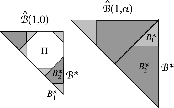
Figure 19: Return orbits for ${\mathcal{B}}\rightarrow{\mathcal{B}}^{*}$, $s=0$ (left) and $s=\alpha$ (right).

Turning now to the other endpoint, we assume ${\mathcal{B}}=\widehat{{\mathcal{B}}}(1,\alpha)$. The data for this dressed domain and its atoms $B_{3}$, $B_{4}$, and $B_{5}$ are displayed in table 1 with $l=1,\;h=\alpha$. By direct iteration of $\rho_{\stackrel{{\scriptstyle}}{{{{\mathcal{B}}}}}}$ on the tiles

$$B^{*}_{1} = \mathtt{T}_{(0,-2\beta)}\mathtt{R}_{5}Q_{1}(\alpha\beta),$$

$$B^{*}_{2} = \mathtt{T}_{(0,-2\alpha)}\mathtt{R}_{3}Q_{7}(2),$$

one verifies that the two orbits tile the spanning domain of ${\mathcal{B}}$ (see figure 19), and produce a return map which promotes $B_{3}$ to a negative-parity dressed domain ${\mathcal{B}}^{*}$ congruent to $\widehat{{\mathcal{B}}}(1,0)$. The incidence matrix is given in Appendix C.

$\Box$

Proof of theorem 1, statement $ii)$, for $i=\pm 1$. The parameter values $s=\Delta_{-1}=\Delta_{0}=\beta$ and $s=\Delta_{1}=1$ are distinguished from the other cases of scenario I by the presence of two higher-level base triangles with disjoint return orbits, both of which are needed to complete the tiling of the parent base triangle. The case $s=\beta$ is proved by direct iteration according to Tiling Plan 2, which is reported in Appendix B and illustrated in figure 20; the treatment of $s=1$ is included in the Electronic Supplement. $\Box$

An important consequence of this is the splitting of the exceptional set into disjoint ergodic components. Such a behaviour, already observed in quadratic two-dimensional piecewise isometries [11] here takes a very simple form. Moreover, infinitely many examples of it appear in our family, corresponding to the set of all accumulation points, at $\beta^{k}$ and $\alpha-\beta^{k},\;k=1,2,\ldots$. (The cases with $k>1$ belong to scenario II, to be treated later.)

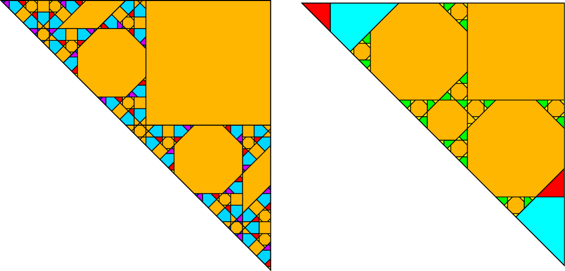
Figure 20: Illustration of the complete tiling of $\mathrm{B}(1,s)$ by the return orbits of the higher-level base triangle(s) and a finite number of periodic domains. The tiling on the left is for $s=107/200\in I_{0,-1}$, while that on the right is for the accumulation point $s=\beta$.

Proof of proposition 2. For all finite $(i,j)$ of scenario I, we prove the renormalization $\mathcal{B}\to\mathcal{B}^{*}$ by direct iteration of the domain map $\rho_{\stackrel{{\scriptstyle}}{{{\mathcal{B}}}}}$. Let us illustrate the salient features of the calculations in the case $(i,j)=(0,-1)$, corresponding to $s\in I_{0,-1}=(\beta+\beta^{3},\alpha\beta]$. The corresponding Tiling Plan 1, shown in Appendix B, has been validated using the procedure specified in section 2.5. Extension of these results to the endpoint $\alpha\beta$ is straightforward, requiring us to ignore those tiles of ${\mathcal{B}}^{*}$ and periodic domains of Tiling Plan 1 which degenerate to lower-dimensional objects, and allow for the possibility of redundant edge conditions in the specification of tile shapes. In the present example, only 6 of the original 14 tiles survive at the endpoint, with ${\mathcal{B}}^{*}$ degenerating to a two-atom right triangle, as it should in accordance with the vanishing of $r(\alpha\beta)$. Even though ${\mathcal{B}}^{*}$ for $s=\alpha\beta$ has only two atoms, their return paths are the same as in the open interval, and their incidence matrix is formed by the first two columns of the $5\times 5$ matrix ${\rm M}(0,-1)$ displayed in Appendix C.

The tiling plans for the remaining $(i,j)$-values of scenario $I$ are analogous. Equivalent data tables will be found in the Electronic Supplement, while the corresponding incidence matrices are listed in Appendix C.

10.3 Proof of $\mathcal{B}\to\mathcal{P}$ (scenarios II and IV)

Scenarios II and IV deal with the peripheral parts of the $s$-interval, namely $s\leqslant\alpha\beta^{2}$ and $s\geqslant\alpha-\alpha\beta^{2}=2\alpha\beta$. In these regions we find asymptotic phenomena, which develop at the accumulation points of the singularities of the renormalization function $r$. The analysis is divided into two cases (see figure 10). In Scenario II, the index $|i|$ diverges while $j$ remains within small bounds, so that $s$ approaches one of the accumulation points $s=0,\alpha$ of $f$, without approaching the first-order accumulation points $s=\beta^{k}$ or $\alpha-\beta^{k}$. Scenario IV deals with larger values of $|j|$, and includes all doubly asymptotic cases: $|i|,|j|\to\infty$. We shall establish the following result (the set IV is defined in (28), p. 28):

Proposition 3

Let $(i,j)\subset{\rm II}\cup{\rm IV}$, let $s\in I_{i,j}$, and let ${\mathcal{B}}\sim\widehat{{\mathcal{B}}}(1,s)$. Then

$${\mathcal{B}}\rightarrow{\mathcal{P}}\sim\widehat{{\mathcal{P}}}(\alpha,s),\;\mbox{with}\;\;\pi({\mathcal{P}})=1.$$ (58)

Moreover,

$${\mathcal{P}}\rightarrow{\mathcal{P}}^{*}\sim\left\{\begin{array}[]{l}\widehat{{\mathcal{P}}}(\beta^{|i|-1}\alpha,s),\quad\mbox{with}\quad\pi({\mathcal{P}}^{*})=(-1)^{|i|-1},\quad\mbox{if}\;\;i\cdot j>0,\\ \widehat{{\mathcal{P}}}(\beta^{|i|-2}\alpha,s),\quad\mbox{with}\quad\pi({\mathcal{P}}^{*})=(-1)^{|i|},\quad\mbox{if}\quad i\cdot j\leq 0.\end{array}\right.$$ (59)

The incidence matrix for the combined renormalization step ${\mathcal{B}}\rightarrow{\mathcal{P}}^{*}$ is given by (62).

Proof. The proof of $(\ref{eq:BP})$, including the calculation of the incidence matrix, is performed separately for the $s$ intervals $(0,\alpha\beta^{3})$, $[\alpha\beta^{3},\alpha\beta^{2}]$, and $[2\alpha\beta,\alpha)$.

Proof of (58) for $s\in(0,\alpha\beta^{3}]$. We prove (58) in two stages. The first, non-branching, stage involves the disjoint return orbits of a fixed number of initial tiles. As $s$ ranges over the interval of interest, the orbits evolve continuously without bifurcations. The second stage of the proof deals with all of the $s$-dependent branching, which is entirely accounted for by the transfer-map dynamics of an arrowhead dressed domain ${\mathcal{A}}=(\mathrm{A},\mathbf{A},\rho_{\stackrel{{\scriptstyle}}{{\mathcal{A}}}})$ congruent to $\widehat{{\mathcal{A}}}(\alpha\beta^{2},s)$.

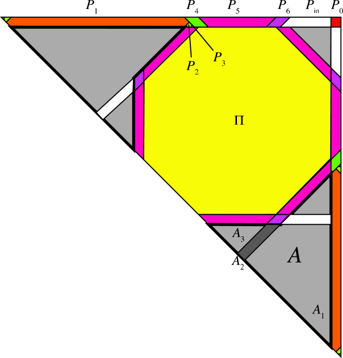
Figure 21: Joint return-map partition of pencil $P$ and arrowhead $A$. Those atoms of the pencil’s return map which reside in the quadrilateral $P_{\rm in}$ are mapped, via three iterations of $\rho_{B}$, into the entrance tile of the arrowhead $A$. The transfer map $\psi(r,h)$ for $A$ then maps them onto the exit tile (dark grey). From there, they are mapped back into $P$ by a single application of $\rho_{B}$.

The non-branching part of the proof establishes the first-return orbits of the disconnected domain ${\rm P}\cup{\rm A}$. This set includes the persistent orbits of $P_{0},\ldots,P_{6}$, which begin and end in ${\rm P}$, never entering the arrowhead. In addition, we have $P_{\rm in}$ (the complement of $\cup_{i=0}^{6}P_{i}$ in ${\rm P}$, ignoring boundaries), whose return orbit ends on the entrance tile of ${\mathcal{A}}$. The set of atoms is rounded out by the three tiles of ${\bf A}$. Of these, $A_{1}$ and $A_{3}$ have orbits which return to ${\rm A}$ without entering ${\rm P}$, while that of $A_{2}$ ends up on ${\tt U}_{0}P_{\rm in}$. All of these statements are proved by direct iteration, with the Tiling Plan 3. We will use the notation $\rho_{\stackrel{{\scriptstyle}}{{{\mathcal{P}},{\mathcal{A}}}}}$ for the joint return map.

It remains to establish the $s$-dependent partition of $P_{\rm in}$ and piecewise isometric mapping of $P_{\rm in}$ under $\rho_{\stackrel{{\scriptstyle}}{{{\mathcal{P}}}}}$. The restriction of the latter to $P_{\rm in}$ is given by

$$\left.\rho_{\stackrel{{\scriptstyle}}{{{\mathcal{P}}}}}\right|_{P_{\rm in}}=\rho_{\stackrel{{\scriptstyle}}{{{\mathcal{P}},{\mathcal{A}}}}}\circ\psi_{\stackrel{{\scriptstyle}}{{{\mathcal{A}}}}}\circ\rho_{\stackrel{{\scriptstyle}}{{{\mathcal{P}},{\mathcal{A}}}}}$$ (60)

where $\psi_{\mathcal{A}}$ is the arrowhead transfer map. According to the Arrowhead Lemma (section 9), the map $\psi_{\stackrel{{\scriptstyle}}{{{\mathcal{A}}}}}$ partitions the entrance tile of ${\mathcal{A}}\sim\widehat{{\mathcal{A}}}(\alpha\beta^{2},s)$ into a strip congruent to $\widehat{\mathbf{S}}(\alpha\beta^{2},s)$. Since $\rho_{\stackrel{{\scriptstyle}}{{{\mathcal{P}},{\mathcal{A}}}}}$ acts on each atom as an orientation-preserving isometry, the atoms contained in $P_{\rm in}$ inherit the strip structure. This is precisely what is needed to fill out the specification of the tiling of ${\mathcal{P}}\sim\widehat{{\mathcal{P}}}(\alpha,s)$. Finally, it is easy to verify that the composition of maps in (60) provides the correct mapping $\rho_{\stackrel{{\scriptstyle}}{{{\mathcal{P}}}}}$ of the atoms in $P_{\rm in}$.

The temporal scaling information of the induction ${\mathcal{B}}\rightarrow{\mathcal{P}}$ is neatly summarized in an incidence matrix ${\rm M}_{\epsilon}({\mathcal{B}}\to{\mathcal{P}})$. For each of the persistent atoms $P_{k},\;k=0,\ldots,6$, one lists in the relevant column of ${\rm M}_{\epsilon}({\mathcal{B}}\to{\mathcal{P}})$ the number of times the return orbit of $P_{k}$ visits each of the five atoms of ${\bf B}$. This information is tallied in the course of the CAP validation. For the remaining atoms, the same data set provides the tile counts for the partial orbits to and from the arrowhead, as well as the the tile counts for the return orbits of the arrowhead atoms. Combining this with the incidence matrix (LABEL:eq:NEk) for the arrowhead transfer map (Arrowhead Lemma, part $iii)$), we obtain the rest of ${\rm M}_{\epsilon}({\mathcal{B}}\to{\mathcal{P}})$. The result is

$${\rm M}_{\epsilon}({\mathcal{B}}\to{\mathcal{P}})=\begin{array}[]{c|ccccccccc}&P_{0}&P_{1}&P_{2}&P_{3}&P_{4}&P_{5}&P_{6}&\lx@intercol\hfil\overbrace{P_{2k-1}\;P_{2k}}^{4\leqslant k\leqslant L}\hfil\lx@intercol\\ \hline\cr B_{1}&0&1&1-\epsilon&1-\epsilon&0&0&0&a_{k}&c_{k}\\ B_{2}&0&0&0&0&1&6&3&b_{k}&d_{k}\\ B_{3}&1&1&1&1&1&1&1&1&1\\ B_{4}&0&0&1&0&0&0&0&0&0\\ B_{5}&0&0&0&1&0&0&0&0&0\end{array}$$ (61)

where $\epsilon=i/|i|$, $L=|i|+3$, and

$$\begin{array}[]{ll}a_{k}=-\frac{1}{2}+(-1)^{k}+\frac{1}{2}\cdot 3^{k-2},&c_{k}=-\frac{1}{2}+\frac{1}{4}(-1)^{k}+\frac{1}{4}\cdot 3^{k-2},\\ b_{k}=1-2(-1)^{k}+3^{k-2},&d_{k}=1-\frac{1}{2}(-1)^{k}+\frac{1}{2}\cdot 3^{k-2}.\end{array}$$

The return times for the pencil’s atoms, expressed in terms of iterations of $\rho_{B}$, are obtained by summing the respective columns of the incidence matrix. We have established the completeness of the tiling by return orbits of the pencil and arrowhead by calculating the total area of each return orbit (area of the source polygon multiplied by the return time), summing over all orbits, including the periodic one, and comparing with the area of ${\rm B}$. Note that it is unnecessary to consider anew the periodic orbits which pass through the arrowhead, since these are subsumed in the recursive tiling property of the arrowhead proved in section 9.

Proof of (58) and (61) for $s\in[\alpha\beta^{3},\alpha\beta^{2}]$. On this interval, the pencil ${\mathcal{P}}$ is minimal, with precisely 9 atoms. Here, the mediation of an arrowhead is not needed, and we prove the renormalization step and incidence matrix using the method of direct iteration. The statement and validation of the tiling scheme (from which the incidence matrix (61) can be verified) may be found in the Electronic Supplement [6].

Proof of (58) for $s\in[2\alpha\beta,\alpha)$. Consider now the relation between a value of $s$ in $(0,\alpha\beta^{2}]$ and its mirror value $\tilde{s}=\alpha-s$. In the latter case, the return-map partition of $B_{3}(\tilde{s})$ (the third atom of $\widehat{{\mathcal{B}}}(1,s)$ in the canonical ordering of table 1) is very far from being pencil-like. On the other hand, one of the five atoms of $B_{3}(\tilde{s})$ is in fact a pencil $\tilde{P}$ with the same parameters and same return-map (up to placement) as $P=B_{3}(s)$.

We first compare explicitly the return orbits of tiles $P_{2}$ and $P_{3}$ to those of $\tilde{P}_{2}$ and $\tilde{P}_{3}$. They are different, but lead to the same image tiles, up to placement, after returning to the pencil.

Now let us remove tiles #2 and #3 from the game and consider how to construct the return orbits of the remaining tiles of each pencil. These orbits will visit only the tiles $B_{1}(s)$ and $B_{2}(s)$ (respectively, $B_{31}(\tilde{s})$ and $B_{32}(\tilde{s})$, the sub-tiles 1 and 2 of $B_{3}(\tilde{s})$) before returning to the pencil, since the remaining two tiles lie on the orbits of tiles #2 and #3. Now $B_{1}(s)$ and $B_{31}(\tilde{s})$ are congruent and the action of the respective mappings on them are the same, up to placement. If the overlaps of $B_{2}(s)$ with the orbits of #2 and #3 are deleted, then the truncated polygon is found to be congruent to $B_{32}(\tilde{s})$, and once again the mappings are the same, up to placement. Thus the return orbits of all the remaining tiles of the two pencils are identical, up to placement. The above arguments are illustrated in figure 22

Figure 22: Return orbits of pencil tiles #2 and #3, shown in boxes against the background of the return-map partitions of $B_{1}(s)$ (on left) and $B_{13}(\tilde{s})$, for a value of $\tilde{s}$ near 1.3. Note that once the two orbits are deleted, the effective domain maps needed to calculate the return orbits of the remaining pencil tiles are conjugate via a rotation and translation.

For the mirror intervals with $s\geqslant 2\alpha\beta$, the ${\mathcal{B}}\rightarrow{\mathcal{P}}$ incidence matrix is again given by (61), with $\epsilon=1$.

Proof of (59). The proof is a direct application of the Pencil Shortening Lemma (section 8.2). Multiplying the incidence matrices for ${\mathcal{B}}\rightarrow{\mathcal{P}}$ and ${\mathcal{P}}\rightarrow{\mathcal{P}}^{*}$, we obtain, for $s\in(0,\alpha\beta^{2}]\cup[2\alpha\beta,\alpha)$,

$${\rm M}_{\epsilon}({\mathcal{B}}\to{\mathcal{P}}^{*})=\left(\begin{array}[]{ccccccccc}0&-\frac{1}{2}&\frac{1}{2}-\epsilon(i)-2|i|&-2&-\frac{1}{2}&-\frac{1}{2}&-\frac{1}{2}&-\frac{1}{2}&-\frac{1}{2}\\ 0&1&4|i|-6&4&1&1&1&1&1\\ 1&1&9&4&1&1&1&1&1\\ 0&0&1&0&0&0&0&0&0\\ 0&0&0&0&0&0&0&0&0\end{array}\right)+$$

$$\left(\begin{array}[]{ccccccccc}0&-1&-\frac{3}{4}&-\frac{3}{2}&-\frac{1}{4}&1&\frac{1}{4}&-1&-\frac{1}{4}\\ 0&2&\frac{3}{2}&3&\frac{1}{2}&-2&-\frac{1}{2}&2&\frac{1}{2}\\ 0&0&0&0&0&0&0&0&0\\ 0&0&0&0&0&0&0&0&0\\ 0&0&0&0&0&0&0&0&0\end{array}\right)\,(-1)^{i}+$$ (62)

$$\left(\begin{array}[]{ccccccccc}0&\frac{1}{6}&\frac{7}{12}&\frac{7}{18}&\frac{1}{12}&\frac{1}{2}&\frac{1}{4}&\frac{3}{2}&\frac{3}{4}\\ 0&\frac{1}{3}&\frac{7}{6}&\frac{7}{9}&\frac{1}{6}&1&\frac{1}{2}&3&\frac{3}{2}\\ 0&0&0&0&0&0&0&0&0\\ 0&0&0&0&0&0&0&0&0\\ 0&0&0&0&0&0&0&0&0\end{array}\right)\,3^{|i|}$$

10.4 Proof of ${\mathcal{P}}^{*}\rightarrow{\mathcal{B}}^{*}$ (scenario II)

Scenario II includes both a countable set of accumulation points, namely $\Delta_{i},\;|i|\geqslant 2$, as well as a subset of the continuity intervals, $I_{i,j}$, $i,j$ finite. In the former case, the renormalization is described by statement (ii) of theorem 1, while the latter case is handled by the following proposition:

Proposition 4

Let $(i,j)\in{\rm II}\cap\mathbb{Z}^{2}$, let $s\in I_{i,j}$, and let ${\mathcal{P}}^{*}$ be as in (59). Then ${\mathcal{P}}^{*}\rightarrow{\mathcal{B}}^{*}$ where

$${\mathcal{B}}^{*}\sim\widehat{{\mathcal{B}}}(l^{*},r(s)l^{*}),\quad\mbox{with}\quad l^{*}=\beta^{|i|+|j|+2},\;\pi({\mathcal{B}}^{*})=(-1)^{|i|+|j|}.$$ (63)

The incidence matrices for this renormalization step are listed in Appendix D.

Proof. Thanks to the scale invariance of the dynamics, it is sufficient to restrict ourselves to the values of $s$ (both the accumulation points and the continuity intervals) where the pencil is minimal. These are handled on a case-by-case basis by direct iteration, exactly as was done for scenario I. Again, we relegate the tiling plans to the Electronic Supplement, with the exception of those for the accumulation points $s=\beta^{k},\;k=2,3,\ldots$, where tiling of the pencil requires two return orbits of higher-level base triangles (see Tiling Plan 4 and figure 23). For the sake of the completeness of the scaling data, we list all the relevant incidence matrices in Appendices D and F.

Figure 23: Tiling of the minimal pencil by two disjoint return orbits of $s=0$ base triangles, plus several periodic orbits.

10.5 Proof of $\mathcal{B}\to\mathcal{T}_{\mu}$ (scenarios III and IV)

Proposition 5

Let $(i,j)\in{\rm III}\cup{\rm IV}$ (see equation (28)), let $s\in I_{i,j}$, and let ${\mathcal{B}}\sim\widehat{{\mathcal{B}}}(1,s)$. Then ${\mathcal{B}}\rightarrow{\mathcal{T}}_{\mu(i,j)}$, where $\mu(i,j)$ is as in table 2 p. 2, and

$${\mathcal{T}}_{-} \sim \widehat{{\mathcal{T}}}_{-}(\beta^{|i|+1},s-\beta^{|i|+1}),\;\mbox{with}\;\pi({\mathcal{T}}_{-})=(-1)^{|i|},$$ (64)

$${\mathcal{T}}_{+} \sim \widehat{{\mathcal{T}}}_{+}(\beta^{|i|+2},\beta^{|i|}-s),\;\;\;\mbox{with}\;\;\pi({\mathcal{T}}_{+})=(-1)^{|i|+1}.$$

The relevant incidence matrices are given in formulae (66)–(71).

Proof. We start with scenario III_μν, with $s\in[\beta-\beta^{6},\beta)\cup(\beta,\beta+\beta^{4}]$, corresponding to $i=0$ for ${\mathcal{T}}_{-}$ and $i=-1$ for ${\mathcal{T}}_{+}$ in (64). Our first task is to prove that the return map for $B_{1}$,the first atom of $\widehat{{\mathcal{B}}}(1,s)$, promotes the triangle to a fringed triangle of type $\widehat{{\mathcal{T}}}_{-}(\beta,s-\beta)$ (resp. $\widehat{{\mathcal{T}}}_{+}(\beta^{3},\beta-s))$. To help establish this, we introduce an auxiliary arrowhead (analogous to that introduced in section 10.3) and prove by direct iteration that the induced domain map is the correct one. The non-branching part of the return-map proof, valid for all $s$ in the chosen interval and illustrated in figure 24, is accomplished with computer assistance, according to the Tiling Plans 5 and 6. There ${\rm T}^{\pm}=B_{1}$, and $T^{-}_{1},\ldots,T^{-}_{4}$ (resp. $T^{-}_{1},\ldots,T^{-}_{7}$) are atoms whose return orbits are non-branching. The domain $T^{\pm}_{\rm in}$ is a ‘blank’ polygon which is delivered by the computer program to the entrance tile of the arrowhead. Arrowhead dynamics endows the polygon with the ($s$-dependent) structure of a strip, and maps it to the exit domain $A_{2}$, from which it is delivered, isometrically to its final destination in ${\rm T}$ by the computer program. The completeness of the tiling is checked by summing the areas of all tiles contained in the computer-generated orbits of the source domains.

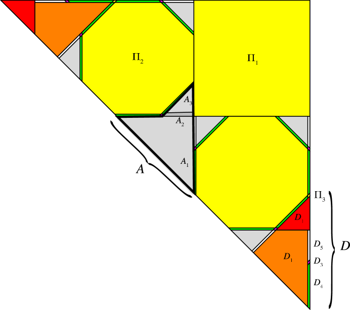
Figure 24: Tiling of the base for scenario III_-ν, according to the Tiling Plan 7.

An analogous treatment for $s$ in the mirror interval $[1-\beta^{4},1+\beta^{6}]$ can be given, with the tiling domain ${\rm T}^{\pm}=B_{5}$, the fifth atom of $\widehat{{\mathcal{B}}}(1,s)$. The tiling schemes, which are very similar to Tiling Plans 5 and 6, have been relegated to the Electronic Supplement. Once again, however, we list all the incidence matrices, using a superscript to indicate the sign of index $i$. Moreover, it is useful, from here on, to introduce a parameter

$$K=|j|-(\mu(i,j)+1)/2.$$ (65)

In the current context, this will be used to keep track of the numbers of atoms in the various parametric dressed domains.

For negative $i$, we have the scenario III incidence matrices

$${\rm M}_{--}({\mathcal{B}}\to{\mathcal{T}})=\begin{array}[]{c|cccc}&T^{-}_{1}&T^{-}_{2}&\lx@intercol\hfil\overbrace{T^{-}_{2k-1}\;T^{-}_{2k}}^{2\leqslant k\leqslant K+2}\hfil\lx@intercol\\ \hline\cr B_{1}&1&1&1&1\\ B_{2}&0&0&a_{k}&c_{k}\\ B_{3}&0&0&b_{k}&d_{k}\\ B_{4}&0&1&2&2\\ B_{5}&1&0&0&0\end{array}$$ (66)

where

$$\begin{array}[]{ll}a_{k}=1+2(-1)^{k}+3^{k-1},&\qquad c_{k}=1+\frac{1}{2}(-1)^{k}+\frac{1}{2}\cdot 3^{k-1},\\ b_{k}=\frac{1}{2}+3(-1)^{k}+\frac{1}{2}\cdot 3^{k-1},&\qquad d_{k}=\frac{1}{2}+\frac{3}{4}(-1)^{k}+\frac{1}{4}\cdot 3^{k-1}.\end{array}$$

$${\rm M}_{-+}({\mathcal{B}}\to{\mathcal{T}})=\begin{array}[]{c|ccccccccc}&T^{+}_{1}&T^{+}_{2}&T^{+}_{3}&T^{+}_{4}&T^{+}_{5}&T^{+}_{6}&T^{+}_{7}&\lx@intercol\hfil\overbrace{T^{+}_{2k}\;T^{+}_{2k+1}}^{4\leqslant k\leqslant K+4}\hfil\lx@intercol\\ \hline\cr B_{1}&1&1&1&1&1&1&1&1&1\\ B_{2}&0&0&0&10&18&2&5&a_{k}&c_{k}\\ B_{3}&0&0&1&7&10&3&4&b_{k}&d_{k}\\ B_{4}&0&1&0&0&0&0&0&0&0\\ B_{5}&1&0&0&0&0&0&0&0&0\end{array}$$ (67)

where

$$\begin{array}[]{ll}a_{k}=17+2(-1)^{k}+3^{k-1},&\qquad c_{k}=17+\frac{1}{2}(-1)^{k}+\frac{1}{2}\cdot 3^{k-1},\\ b_{k}=\frac{17}{2}+3(-1)^{k}+\frac{1}{2}3^{k-1},&\qquad d_{k}=\frac{17}{2}+\frac{3}{4}(-1)^{k}+\frac{1}{4}\cdot 3^{k-1}.\end{array}$$

For positive $i$, the corresponding matrices are

$${\rm M}_{+-}({\mathcal{B}}\to{\mathcal{T}})=\begin{array}[]{c|cccc}&T^{-}_{1}&T^{-}_{2}&\lx@intercol\hfil\overbrace{T^{-}_{2k-1}\;T^{-}_{2k}}^{2\leqslant k\leqslant K+2}\hfil\lx@intercol\\ \hline\cr B_{1}&1&0&0&0\\ B_{2}&0&1&2&2\\ B_{3}&0&0&a_{k}&c_{k}\\ B_{4}&0&0&b_{k}&d_{k}\\ B_{5}&1&1&1&1\end{array}$$ (68)

where

$$\begin{array}[]{ll}a_{k}=\frac{1}{2}+5(-1)^{k}+\frac{1}{2}3^{k},&\qquad c_{k}=\frac{1}{2}+\frac{5}{4}(-1)^{k}+\frac{1}{4}3^{k},\\ b_{k}=1+2(-1)^{k}+3^{k-1},&\qquad d_{k}=1+\frac{1}{2}(-1)^{k}+\frac{1}{2}\cdot 3^{k-1}.\end{array}$$

$${\rm M}_{++}({\mathcal{B}}\to{\mathcal{T}})=\begin{array}[]{c|ccccccccc}&T^{+}_{1}&T^{+}_{2}&T^{+}_{3}&T^{+}_{4}&T^{+}_{5}&T^{+}_{6}&T^{+}_{7}&\lx@intercol\hfil\overbrace{T^{+}_{2k}\;T^{+}_{2k+1}}^{4\leqslant k\leqslant K+4}\hfil\lx@intercol\\ \hline\cr B_{1}&1&0&0&0&0&0&0&0&0\\ B_{2}&0&1&0&0&0&0&0&0&0\\ B_{3}&0&0&2&18&29&6&10&a_{k}&c_{k}\\ B_{4}&0&0&0&10&18&2&5&b_{k}&d_{k}\\ B_{5}&1&1&1&1&1&1&1&1&1\end{array}$$ (69)

where

$$\begin{array}[]{ll}a_{k}=\frac{53}{2}+5(-1)^{k}+\frac{1}{2}3^{k},&\qquad c_{k}=\frac{53}{2}+\frac{5}{4}(-1)^{k}+\frac{1}{4}3^{k},\\ b_{k}=17+2(-1)^{k}+3^{k-1},&\qquad d_{k}=17+\frac{1}{2}(-1)^{k}+\frac{1}{2}\cdot 3^{k-1}.\end{array}$$

We now turn to scenario IV_μν, where the renormalization process has already reached the minimal pencil stage. The next step, in which fringed triangles are induced, is completely analogous to what we have just studied for ${\mathcal{B}}\rightarrow{\mathcal{T}}_{\mu}$, again leading to (64). The relevant Tiling Plans 7 and 8 are given in Appendix B for the two values of $\mu$.

The corresponding incidence matrices are:

$${\rm M}_{-}({\mathcal{P}}^{*}\to{\mathcal{T}})=\begin{array}[]{c|ccccccc}&T^{-}_{1}&T^{-}_{2}&T^{-}_{3}&T^{-}_{4}&\lx@intercol\hfil\overbrace{T^{-}_{2k-1}\;T^{-}_{2k}}^{3\leqslant k\leqslant K+2}\hfil\lx@intercol\\ \hline\cr P^{*}_{0}&0&0&0&0&0&0\\ P^{*}_{1}&0&0&0&0&0&0\\ P^{*}_{2}&0&1&2&2&2&2\\ P^{*}_{3}&0&0&0&0&0&0\\ P^{*}_{4}&2&2&4&4&4&4\\ \ P^{*}_{5}&1&1&1&1&1&1\\ P^{*}_{6}&0&0&6&3&a_{k}&d_{k}\\ P^{*}_{7}&0&0&0&0&b_{k}&e_{k}\\ P^{*}_{8}&0&0&0&0&c_{k}&f_{k}\\ \end{array}$$ (70)

where

$$\begin{array}[]{ll}a_{k}=1+2(-1)^{k}+3^{k-2},&\qquad d_{k}=1+\frac{1}{2}(-1)^{k}+\frac{1}{2}\cdot 3^{k-2},\\ b_{k}=-\frac{1}{2}-(-1)^{k}+\frac{1}{2}\cdot 3^{k-3},&\qquad e_{k}=-\frac{1}{2}-\frac{1}{4}(-1)^{k}+\frac{1}{4}\cdot 3^{k-3},\\ c_{k}=1+2(-1)^{k}+3^{k-3},&\qquad f_{k}=1+\frac{1}{2}(-1)^{k}+\frac{1}{2}\cdot 3^{k-3},\end{array}$$

$${\rm M}_{+}({\mathcal{P}}^{*}\to{\mathcal{T}})=\begin{array}[]{c|cccccccccccc}&T^{+}_{1}&T^{+}_{2}&T^{+}_{3}&T^{+}_{4}&T^{+}_{5}&T^{+}_{6}&T^{+}_{7}&\lx@intercol\hfil\overbrace{T^{+}_{2k}\;T^{+}_{2k+1}}^{4\leqslant k\leqslant K+4}\hfil\lx@intercol\\ \hline\cr P^{*}_{0}&0&0&0&0&0&0&0&0&0\\ P^{*}_{1}&0&0&0&0&0&0&0&0&0\\ P^{*}_{2}&0&1&0&0&0&0&0&0&0\\ P^{*}_{3}&0&0&0&0&0&0&0&0&0\\ P^{*}_{4}&2&2&0&0&0&0&0&0&0\\ \ P^{*}_{5}&1&1&1&1&1&1&1&1&1\\ P^{*}_{6}&0&0&0&4&6&2&2&a_{k}&d_{k}\\ P^{*}_{7}&0&0&0&0&1&0&0&b_{k}&e_{k}\\ P^{*}_{8}&0&0&0&2&2&0&1&c_{k}&f_{k}\\ \end{array}$$ (71)

where

$$\begin{array}[]{ll}a_{k}=5+2(-1)^{k}+3^{k-2},&\qquad d_{k}=5+\frac{1}{2}(-1)^{k}+\frac{1}{2}\cdot 3^{k-2},\\ b_{k}=\frac{3}{2}-(-1)^{k}+\frac{1}{2}\cdot 3^{k-3},&\qquad e_{k}=\frac{3}{2}-\frac{1}{4}(-1)^{k}+\frac{1}{4}\cdot 3^{k-3},\\ c_{k}=1+2(-1)^{k}+3^{k-3},&\qquad f_{k}=1+\frac{1}{2}(-1)^{k}+\frac{1}{2}\cdot 3^{k-3}.\end{array}$$

10.6 Proof of ${\mathcal{T}}_{\mu}\rightarrow{\mathcal{D}}_{\mu}\rightarrow{\mathcal{D}}_{\nu}^{*}$ (scenarios III and IV)

The next phase of scenarios III_μν and IV_μν is the transition from fringed triangle to double-strip, followed by shortening of the strip.

Proposition 6

Let $(i,j)\in{\rm III}\cup{\rm IV}$, let $s\in I_{i,j}$, and let ${\mathcal{T}}_{\mu(i,j)}$ be as in (64). Then ${\mathcal{T}}_{\mu(i,j)}\rightarrow{\mathcal{D}}_{\mu(i,j)}$, where

$${\mathcal{D}}_{-} \sim \widehat{{\mathcal{D}}}_{-}(\beta^{|i|+3},s-\beta^{|i|+1}),\;\mbox{with}\;\pi({\mathcal{D}}_{-})=(-1)^{|i|+1},$$ (72)

$${\mathcal{D}}_{+} \sim \widehat{{\mathcal{D}}}_{+}(\beta^{|i|+4},\beta^{|i|}-s),\;\;\;\mbox{with}\;\;\pi({\mathcal{D}}_{+})=(-1)^{|i|},$$

and the corresponding incidence matrices are given in (75) and (74), Moreover,

$${\mathcal{D}}_{\mu(i,j)}\rightarrow{\mathcal{D}}^{*}_{\nu(j)}\sim\left\{\begin{array}[]{ll}\widehat{{\mathcal{D}}}_{\nu(j)}(\beta^{|i|+|j|},s-\beta^{|i|+1}),&\;\mbox{if}\;\mu(i,j)=-1,\\ \widehat{{\mathcal{D}}}_{\nu(j)}(\beta^{|i|+|j|},\beta^{|i|}-s),&\;\mbox{if}\;\mu(i,j)=+1,\end{array}\right.$$ (73)

with $\pi({\mathcal{D}}^{*}_{\nu(j)})=(-1)^{|i|+|j|}$.

Proof of (72). We begin with the case $\mu(i,j)=-1$. Our task is to calculate the return-map orbits of the trapezoidal atom $T^{-}_{3}$ of the fringed triangle (see figure 13), showing that the corresponding partition is that of a double-strip with the stated parameters. Scale invariance allows us to fix the parameter $l$ of the fringed triangle at $l=\beta$ and let the parameter $h$ range over $(0,\beta^{4}]$. This treats simultaneously all integer values of the index $i$.

The non-branching part of the proof consists of the computer-assisted validation of tiling plan 9 in Appendix B, illustrated in figure 25.

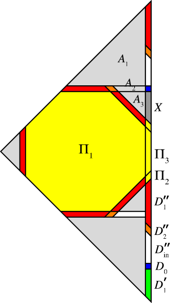
Figure 25: Tiling of the triangle ${\rm T}_{-}$, according to the Tiling Plan 9.

It is worth noting that the induced return map of the double strip corresponds to the variant $\nu=-1$ (since the double strip has negative parity and a net rotation ${\tt R}_{2}$ of atom $D_{0}$).

Once again, arrowhead dynamics is responsible for all of the branching, but with an important difference from previous stages of the renormalization. The double strip, labelled ${\mathcal{D}}_{-}$, has two constituent strips, produced by separate $s$-dependent branching mechanisms. One of these is associated with the arrowhead, while the other is produced by the already established piecewise isometry of proposition 5. It should be emphasized that, as always, computer assistance is enlisted only for the non-branching orbit pieces which are present for all $s$ in the chosen interval. This includes the isometric mapping of $D^{\prime}$ onto $X$, but not the mapping of $X$ back into ${\rm D}$ which completes the return orbit.

The case $\mu(i,j)=+1$ is handled in an analogous manner, with the non-branching part of the proof consisting of computer-assisted validation of tiling plan 10. There we identify two special tiles congruent to $D^{\prime}$, namely $X$ and $Y$. The isometric mappings from $D^{\prime}$ to $X$ and from $Y$ to $D^{\prime}\oslash{\rm D}$ are included in the tiling plan, while the mapping from $X$ to $Y$ is a direct application of the domain map of the fringed triangle.

As a by-product of the return-map calculations leading to (72), we obtain the following incidence matrices:

$${\rm M}_{-}({\mathcal{T}}\to{\mathcal{D}})=\begin{array}[]{c|cccc}&D_{0}&\lx@intercol\hfil\overbrace{D^{{}^{\prime\prime}}_{2k-1}\;D^{{}^{\prime\prime}}_{2k}}^{1\leqslant j\leqslant K}\hfil\lx@intercol&\overbrace{D^{\prime}_{l}}^{1\leqslant l\leqslant 2K-2}\\ \hline\cr T^{-}_{1}&1&a_{k}&c_{k}&0\\ T^{-}_{2}&0&b_{k}&d_{k}&0\\ T^{-}_{3}&1&1&1&1\\ T^{-}_{4}\cdots T^{-}_{6}&0&0&0&0\\ \underbrace{T^{-}_{j+6}}_{1\leqslant j\leqslant 2K-2}&0&0&0&\delta_{jl}\end{array}$$ (74)

where

$$\begin{array}[]{ll}a_{k}=\frac{3}{2}-(-1)^{k}+\frac{1}{2}3^{k-1},&\qquad c_{k}=\frac{3}{2}-\frac{1}{4}(-1)^{k}+\frac{1}{4}\cdot 3^{k}\\ b_{k}=-1+2(-1)^{k}+3^{k-1}&\qquad d_{k}=-1+\frac{1}{2}(-1)^{k}+\frac{1}{2}\cdot 3^{k-1}\end{array}$$

$${\rm M}_{+}({\mathcal{T}}\to{\mathcal{D}})=\begin{array}[]{c|cccc}&D_{0}&\lx@intercol\hfil\overbrace{D^{{}^{\prime\prime}}_{2k-1}\;D^{{}^{\prime\prime}}_{2k}}^{1\leqslant j\leqslant K}\hfil\lx@intercol&\overbrace{D^{\prime}_{l}}^{1\leqslant l\leqslant 2K-2}\\ \hline\cr T^{+}_{1}&0&a_{k}&c_{k}&0\\ T^{+}_{2}&12&b_{k}&d_{k}&12\\ T^{+}_{3}&0&0&0&0\\ T^{+}_{4}&0&2&2&0\\ T^{+}_{5}&1&0&0&0\\ T^{+}_{6}&0&0&0&0\\ T^{+}_{7}&0&0&0&0\\ T^{+}_{8}&1&1&1&1\\ T^{+}_{9}\cdots T^{+}_{11}&0&0&0&0\\ \underbrace{T^{+}_{j+11}}_{1\leqslant j\leqslant 2K-2}&0&0&0&\delta_{jl}\end{array}$$ (75)

where

$$\begin{array}[]{ll}a_{k}=-\frac{1}{2}+(-1)^{k}+\frac{1}{2}3^{k+2},&\qquad c_{k}=-\frac{1}{2}+\frac{1}{4}(-1)^{k}+\frac{1}{4}3^{k+2},\\ b_{k}=13-2(-1)^{k}+3^{k+2},&\qquad d_{k}=13-\frac{1}{2}(-1)^{k}+\frac{1}{2}\cdot 3^{k+2}.\end{array}$$

Proof of (73). We apply the Double-Strip Shortening Lemma (section 8.4) to reduce the number of atoms in the double strip from $4K-1$ to 11 in $k=K-3$ steps. Since $K=|j|-(\mu(i,j)+1)/2$, we have

$$k=|j|-3-\frac{1}{2}(\mu(i,j)+1)=|j|-\left\{\begin{array}[]{ll}3&\mu(i,j)=-1,\\ 4&\mu(i,j)=+1.\end{array}\right.$$

Since as a result of the shortening, the first argument of ${\mathcal{D}}_{\mu}(l,h)$ decreases by a factor $\beta^{k}$ and the parity is multiplied by $(-1)^{k}$, we see that (73) follows from (72).

10.7 Proof of ${\mathcal{D}}^{*}_{\nu}\to{\mathcal{B}}^{*}$ (scenarios III and IV)

This is the final stage of scenarios III_μν and IV_μν.

Proposition 7

Let $(i,j)\subset{\rm III}\cup{\rm IV}$, let $s\in I_{i,j}$, and let ${\mathcal{D}}^{*}_{\nu}$ be as in (73). Then

$${\mathcal{D}}^{*}_{\nu}\rightarrow{\mathcal{B}}^{*}\sim\widehat{{\mathcal{B}}}(l^{*},r(s)l^{*}),\;\mbox{with}\;\;l^{*}=\beta^{|i|+|j|+2},\;\pi({\mathcal{B}}^{*})=(-1)^{|i|+|j|}.$$ (76)

The corresponding incidence matrices are given in (77).

Proof. Setting

$$h=\left\{\begin{array}[]{ll}s-\beta^{|i|+1}&\mu(i,j)=-1,\\ \beta^{|i|}-s&\mu(i,j)=+1,\end{array}\right.$$

we rescale both arguments of $\widehat{{\mathcal{D}}}_{\nu}$ in (73) by a factor $\beta^{3-|i|-|j|}$ to obtain

$$\widehat{{\mathcal{D}}}_{\nu}(\beta^{3},h^{\prime}),\quad h^{\prime}\in[\beta^{5},\beta^{4}],$$

$$h^{\prime}=\beta^{3-|i|-|j|}h.$$

For both values of $\nu$, we have shown by direct iteration (see tiling plans 11 and 12 and figure 26) that the induced return map on the tile $D^{\prime}_{1}$ of the minimal double strip is that of a base triangle of the same parity, namely

$$\widehat{{\mathcal{D}}}_{\nu}(\beta^{3},h^{\prime})\rightarrow{\mathcal{B}}_{\nu}\sim\widehat{B}(\beta^{5},\beta^{4}-h^{\prime}).$$

To complete the proof, we undo the scale transformation, multiplying both arguments of $\widehat{{\mathcal{D}}}_{\nu}$ and $\widehat{B}$ by the same factor $\beta^{|i|+|j|-3}$, and returning to the variable $s$. The result is equation (76). $\Box$

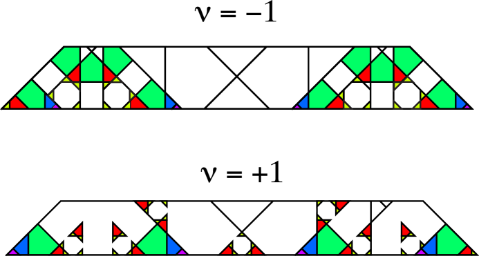
Figure 26: Tiling of the minimal double strip ${\mathcal{D}}*_{\nu}$ for $s=87/200$ ($\nu=-1$) and $s=211/500$ ($\nu=+1$).

The incidence matrices for ${\mathcal{D}}^{*}_{\pm}\rightarrow{\mathcal{B}}^{*}$ are:

$$\begin{array}[]{ccc}{\rm M}_{-}({\mathcal{D}}^{*}\to{\mathcal{B}}^{*})=&&{\rm M}_{+}({\mathcal{D}}^{*}\to{\mathcal{B}}^{*})=\\ \\ \begin{array}[]{c|ccccc}&B^{*}_{1}&B^{*}_{2}&B^{*}_{3}&B^{*}_{4}&B^{*}_{5}\\ \hline\cr D^{*}_{0}&10&4&1&0&0\\ D^{*^{\prime\prime}}_{1}&10&4&2&2&2\\ D^{*^{\prime\prime}}_{2}&10&4&0&0&0\\ D^{*^{\prime\prime}}_{3}&0&0&0&0&0\\ D^{*^{\prime\prime}}_{4}&0&0&0&0&0\\ D^{*^{\prime\prime}}_{5}&0&0&0&0&1\\ D^{*^{\prime\prime}}_{6}&0&0&0&1&0\\ D^{*^{\prime}}_{1}&1&1&1&1&1\\ D^{*^{\prime}}_{2}&4&1&0&0&0\\ D^{*^{\prime}}_{3}&0&0&0&0&0\\ D^{*^{\prime}}_{4}&0&0&0&0&0\end{array}&&\begin{array}[]{c|ccccc}&B^{*}_{1}&B^{*}_{2}&B^{*}_{3}&B^{*}_{4}&B^{*}_{5}\\ \hline\cr D^{*}_{0}&5&2&2&0&0\\ D^{*^{\prime\prime}}_{1}&10&4&5&2&2\\ D^{*^{\prime\prime}}_{2}&0&0&0&0&0\\ D^{*^{\prime\prime}}_{3}&0&0&0&0&0\\ D^{*^{\prime\prime}}_{4}&0&0&0&0&0\\ D^{*^{\prime\prime}}_{5}&0&0&0&0&1\\ D^{*^{\prime\prime}}_{6}&0&0&0&1&0\\ D^{*^{\prime}}_{1}&1&1&1&1&1\\ D^{*^{\prime}}_{2}&4&1&2&0&0\\ D^{*^{\prime}}_{3}&0&0&0&0&0\\ D^{*^{\prime}}_{4}&0&0&0&0&0\end{array}\end{array}$$ (77)

10.8 Conclusion of the proof

We have now proved all of the induction steps comprising the renormalization graph of figure 8. By composing the relevant return maps along the ten closed circuits of the graph, we can now assign to each of the $s$-parametric intervals $I_{i,j}$ a renormalization of the class of base triangles congruent to $\widehat{{\mathcal{B}}}(l,h)$, with $s=h/l\in I_{i,j}$, renormalization functions $\kappa$ and $r$, and parities as prescribed by theorem 1.

The proof of each induction step, via either the Shortening Lemmas of section 8 or the propositions of section 10, yield as by-products a verification of a uniform return path for each pair $(i,j)$, as well as explicit formulae for the incidence matrices.

By composing the tilings of the individual induction steps, one obtains for each $(i,j)$ a tiling of the parent base triangle. This tiling consists of the return orbits of the atoms of the higher-level base triangle, as well as those of finitely many periodic tiles explicitly identified in the proof. For any $(i,j)\in\mathbb{Z}^{2}$, the tile coordinates are all affine functions of $s$. The exhaustiveness of the tiling for each step, hence for the full renormalization, has been established by evaluation of area sums, included in the Electronic Supplement [6].

The proof of theorem 1 is now complete. $\Box$

11 Incidence matrices

Theorem 1 contains a statement asserting the constancy of the incidence matrix on each parameter interval $I_{i,j}$. We did not provide explicit expressions for the incidence matrices, due to the inherently complicated nature of the return-map dynamics. In section 10, we saw how the ten qualitatively distinct routes from initial ${\mathcal{B}}$ to final ${\mathcal{B}}^{*}$ all led to a simple spatial scaling factor $\beta^{|i|+|j|+2}$ and a simple parity-changing factor $(-1)^{|i|+|j|}$. No comparable simplicity can be extracted from the incidence matrices sprinkled throughout the proof of section 10, as they are strongly scenario-dependent. In particular, the incidence matrices vary from interval to interval in a complicated way, breaking the symmetry under $(i,j)\mapsto(-i,-j)$ enjoyed by the spatial scaling and parity-changing factors.

In section 10, we computed the incidence matrices associated with all of the edges of the renormalization graph. For scenarios I and II, we displayed (in appendices C and D) the explicit $5\times 5$ matrices associated with a number of individual intervals and sequences of intervals. On the other hand, for scenarios III and IV, we presented the relevant incidences matrices for individual induction steps, but made no attempt at assembling these into all-embracing formulae. The goal of the present section is to derive such formulae and examine some of their implications.

11.1 Composite formulae for scenarios III and IV

We begin by deriving a concise representation for the incidence matrices associated with the composite renormalization step ${\mathcal{B}}\to{\mathcal{D}}_{\mu}$. Similar treatment will be given for ${\mathcal{P}}^{*}\to{\mathcal{D}}_{\mu}$.

Proposition 8

Let $(i,j)\in{\rm III}$, let $s\in I_{i,j}$, and let ${\rm M}=\mathrm{M}^{\mathrm{III}}_{\epsilon,\mu}({\mathcal{B}}\to{\mathcal{D}})$. Further, let $K$ be given by (65). Then for $k=1,\ldots,K,\;l=1,\ldots,K-1$, the column vectors ${\rm M}_{\mathbf{B},D}$ of the matrix ${\rm M}$ (with $\mathbf{B}=(B_{1},\ldots,B_{5})^{T}$) may be written as follows:

$${\rm M}_{{\bf B},D_{0}} = {\bf X}_{0},$$

$${\rm M}_{{\bf B},D^{{}^{\prime\prime}}_{2k-1}} = {\bf X}^{{}^{\prime\prime}}+4\times(-1)^{k}\,{\bf Y}^{{}^{\prime\prime}}+2\times 3^{k}\,{\bf Z}^{{}^{\prime\prime}},$$

$${\rm M}_{{\bf B},D^{{}^{\prime\prime}}_{2k}} = {\bf X}^{{}^{\prime\prime}}+(-1)^{k}\,{\bf Y}^{{}^{\prime\prime}}+3^{k}\,{\bf Z}^{{}^{\prime\prime}},$$ (78)

$${\rm M}_{{\bf B},D^{{}^{\prime}}_{2k-1}} = {\bf X}^{{}^{\prime}}+4\times(-1)^{k}\,{\bf Y}^{{}^{\prime}}+2\times 3^{k}\,{\bf Z}^{{}^{\prime}},$$

$${\rm M}_{{\bf B},D^{{}^{\prime}}_{2k}} = {\bf X}^{{}^{\prime}}+(-1)^{k}\,{\bf Y}^{{}^{\prime}}+3^{k}\,{\bf Z}^{{}^{\prime}}.$$

Proof. One verifies the formulae by explicitly calculating

$${\rm M}={\rm M}_{\epsilon,\mu}({\mathcal{B}}\to{\mathcal{T}})\cdot{\rm M}_{\mu}({\mathcal{T}}\to{\mathcal{D}}).$$

The results are listed in the following tables:

$$\begin{array}[]{|c|c|c|c|c|c|c||c|c|c|c|c|c|c|}\hline\cr\vrule\lx@intercol\hfil\epsilon=-1,\mu=-1\hfil\lx@intercol\vrule\lx@intercol\vrule\lx@intercol&\vrule\lx@intercol\hfil\epsilon=-1,\mu=+1\hfil\lx@intercol\vrule\lx@intercol\\ \hline\cr{\bf X}_{0}&{\bf X}^{{}^{\prime\prime}}&{\bf Y}^{{}^{\prime\prime}}&{\bf Z}^{{}^{\prime\prime}}&{\bf X}^{{}^{\prime}}&{\bf Y}^{{}^{\prime}}&{\bf Z}^{{}^{\prime}}&{\bf X}_{0}&{\bf X}^{{}^{\prime\prime}}&{\bf Y}^{{}^{\prime\prime}}&{\bf Z}^{{}^{\prime\prime}}&{\bf X}^{{}^{\prime}}&{\bf Y}^{{}^{\prime}}&{\bf Z}^{{}^{\prime}}\\ \hline\cr 2&\frac{3}{2}&-\frac{1}{4}&\frac{3}{4}&2&0&0&14&\frac{31}{2}&-\frac{1}{4}&\frac{27}{4}&14&0&0\\ 6&6&0&0&7&-\frac{1}{2}&\frac{9}{2}&64&66&0&0&63&-\frac{1}{2}&\frac{81}{2}\\ 5&5&0&0&\frac{11}{2}&-\frac{3}{4}&\frac{9}{4}&35&39&0&0&\frac{67}{2}&-\frac{3}{4}&\frac{81}{4}\\ 2&1&-\frac{1}{2}&\frac{1}{2}&4&0&0&12&13&-\frac{1}{2}&\frac{9}{2}&12&0&0\\ 1&\frac{3}{2}&\frac{1}{4}&\frac{1}{4}&0&0&0&0&-\frac{1}{2}&\frac{1}{4}&\frac{9}{4}&0&0&0\\ \hline\cr\end{array}$$

$$\begin{array}[]{|c|c|c|c|c|c|c||c|c|c|c|c|c|c|}\hline\cr\vrule\lx@intercol\hfil\epsilon=+1,\mu=-1\hfil\lx@intercol\vrule\lx@intercol\vrule\lx@intercol&\vrule\lx@intercol\hfil\epsilon=+1,\mu=+1\hfil\lx@intercol\vrule\lx@intercol\\ \hline\cr{\bf X}_{0}&{\bf X}^{{}^{\prime\prime}}&{\bf Y}^{{}^{\prime\prime}}&{\bf Z}^{{}^{\prime\prime}}&{\bf X}^{{}^{\prime}}&{\bf Y}^{{}^{\prime}}&{\bf Z}^{{}^{\prime}}&{\bf X}_{0}&{\bf X}^{{}^{\prime\prime}}&{\bf Y}^{{}^{\prime\prime}}&{\bf Z}^{{}^{\prime\prime}}&{\bf X}^{{}^{\prime}}&{\bf Y}^{{}^{\prime}}&{\bf Z}^{{}^{\prime}}\\ \hline\cr 1&\frac{3}{2}&\frac{1}{4}&\frac{1}{4}&0&0&0&0&-\frac{1}{2}&\frac{1}{4}&\frac{9}{4}&0&0&0\\ 2&1&-\frac{1}{2}&\frac{1}{2}&4&0&0&12&13&-\frac{1}{2}&\frac{9}{2}&12&0&0\\ 10&10&0&0&\frac{21}{2}&-\frac{5}{4}&\frac{27}{4}&101&108&0&0&\frac{197}{2}&-\frac{5}{4}&\frac{243}{4}\\ 6&6&0&0&7&-\frac{1}{2}&\frac{9}{2}&64&66&0&0&63&-\frac{1}{2}&\frac{81}{2}\\ 2&\frac{3}{2}&-\frac{1}{4}&\frac{3}{4}&2&0&0&14&\frac{31}{2}&-\frac{1}{4}&\frac{27}{4}&14&0&0\\ \hline\cr\end{array}$$

We now calculate, using (32)–(35), and (78), the matrix $\tilde{\rm M}$ and column vector ${\rm N}$ such that

$${\rm M}^{\rm III}_{\epsilon,\mu,\nu}({\mathcal{B}}\to{\mathcal{D}}^{*})={\rm M}^{\rm III}_{\epsilon,\mu}({\mathcal{B}}\to{\mathcal{D}})\cdot{\rm M}_{\mu,\nu}({\mathcal{D}}\to{\mathcal{D}}^{*})=\tilde{\rm M}+{\rm N}\cdot(\underbrace{1,1,\ldots,1}_{11}).$$

where, for $K$ even, we have

$$\begin{array}[]{lll}\tilde{\rm M}_{{\bf B},D^{*}_{0}}&=&{\rm M}_{{\bf B},D_{0}}={\bf X}_{0},\\ \vskip 1.0pt\cr\tilde{\rm M}_{{\bf B},D^{*^{\prime\prime}}_{k}}&=&{\rm M}_{{\bf B},D^{\prime}_{2K+k-8}}\\ &=&\left\{\begin{array}[]{ll}{\bf X}^{\prime}+4\times(-1)^{\frac{k-7}{2}}\,{\bf Y}^{\prime}+2\times 3^{K+\frac{k-7}{2}}\,{\bf Z}^{\prime},&k=1,3,5,\\ {\bf X}^{\prime}+(-1)^{\frac{k-8}{2}}\,{\bf Y}^{\prime}+3^{K+\frac{k-8}{2}}\,{\bf Z}^{\prime},&k=2,4,6,\end{array}\right.\\ \vskip 1.0pt\cr\tilde{\rm M}_{{\bf B},D^{*^{\prime}}_{l}}&=&{\rm M}_{{\bf B},D^{{}^{\prime\prime}}_{2K+l-4}}\\ &=&\left\{\begin{array}[]{ll}{\bf X}^{{}^{\prime\prime}}+4\times(-1)^{\frac{l-7}{2}}\,{\bf Y}^{{}^{\prime\prime}}+2\times 3^{K+\frac{l-3}{2}}\,{\bf Z}^{{}^{\prime\prime}},&l=1,3,\\ {\bf X}^{{}^{\prime\prime}}+(-1)^{\frac{l-8}{2}}{\bf Y}^{{}^{\prime\prime}}+3^{K+\frac{l-4}{2}}\,{\bf Z}^{{}^{\prime\prime}},&l=2,4,\end{array}\right.\end{array}$$

$${\rm N}_{\bf B}=\xi_{K+1}({\bf X}^{{}^{\prime\prime}}-4\,{\bf Y}^{{}^{\prime\prime}})+2\,\eta_{K+1}{\bf Z}^{{}^{\prime\prime}}+\xi_{K-1}(2\,{\bf X}^{{}^{\prime}}-8\,{\bf Y}^{{}^{\prime}})+4\,\eta_{K-1}{\bf Z}^{{}^{\prime}},$$

where, using the summation formula for geometric series,

$$\xi_{K}=\sum^{\frac{K-5}{2}}_{l=0}4^{l}=-\frac{1}{3}+\frac{1}{24}\,2^{K},\qquad\eta_{K}=\sum^{\frac{K-5}{2}}_{l=0}4^{l}\,3^{K-4-2l}=\frac{1}{45}\,3^{K}-\frac{3}{40}\,2^{K}.$$

For $K$ odd, we find

$$\begin{array}[]{lll}\tilde{\rm M}_{{\bf B},D^{*}_{0}}&=&{\rm M}_{{\bf B},D_{0}}={\bf X}_{0},\\ \vskip 1.0pt\cr\tilde{\rm M}_{{\bf B},D^{*^{\prime\prime}}_{k}}&=&{\rm M}_{{\bf B},D^{{}^{\prime\prime}}_{2K+k-6}}\\ &=&\left\{\begin{array}[]{ll}{\bf X}^{{}^{\prime\prime}}-4\times(-1)^{\frac{k-5}{2}}\,{\bf Y}^{{}^{\prime\prime}}+2\times 3^{K+\frac{k-5}{2}}\,{\bf Z}^{{}^{\prime\prime}},&k=1,3,5,\\ {\bf X}^{{}^{\prime\prime}}-(-1)^{\frac{k-6}{2}}\,{\bf Y}^{{}^{\prime\prime}}+3^{K+\frac{k-6}{2}}{\bf Z}^{{}^{\prime\prime}},&k=2,4,6,\end{array}\right.\\ \vskip 1.0pt\cr\tilde{\rm M}_{{\bf B},D^{*^{\prime}}_{l}}&=&{\rm M}_{{\bf B},D^{{}^{\prime}}_{2K+l-6}}\\ &=&\left\{\begin{array}[]{ll}{\bf X}^{{}^{\prime}}-4\times(-1)^{\frac{l-5}{2}}\,{\bf Y}^{{}^{\prime}}+4\times 3^{K+\frac{l-5}{2}}\,{\bf Z}^{{}^{\prime}}\,,&l=1,3,\\ {\bf X}^{{}^{\prime}}-(-1)^{\frac{l-5}{2}}\,{\bf Y}^{{}^{\prime}}+3^{K+\frac{l-6}{2}}\,{\bf Z}^{{}^{\prime}},&l=2,4,\end{array}\right.\\ \vskip 1.0pt\cr{\rm N}_{\bf B}&=&\xi_{K}(2\,{\bf X}^{{}^{\prime}}-8\,{\bf Y}^{{}^{\prime}}+{\bf X}^{{}^{\prime\prime}}-4\,{\bf Y}^{{}^{\prime\prime}})+\eta_{K}(4\,{\bf Z}^{{}^{\prime}}+2\,{\bf Z}^{{}^{\prime\prime}}).\end{array}$$

The above formulae can also be used for calculating incidence matrices for ${\mathcal{P}}^{*}\rightarrow{\mathcal{D}}^{*}$, with the index set ${\bf B}$ replaced by ${\bf P}^{*}$ and the vectors ${\bf X}_{0}$, ${\bf X}^{{}^{\prime}}_{k}$, etc., now having nine components, taken from the following tables.

$$\begin{array}[]{|c|c|c|c|c|c|c||c|c|c|c|c|c|c|}\hline\cr\vrule\lx@intercol\hfil\mu=+1\hfil\lx@intercol\vrule\lx@intercol\vrule\lx@intercol&\vrule\lx@intercol\hfil\mu=-1\hfil\lx@intercol\vrule\lx@intercol\\ \hline\cr{\bf X}_{0}&{\bf X}^{{}^{\prime\prime}}&{\bf Y}^{{}^{\prime\prime}}&{\bf Z}^{{}^{\prime\prime}}&{\bf X}^{{}^{\prime}}&{\bf Y}^{{}^{\prime}}&{\bf Z}^{{}^{\prime}}&{\bf X}_{0}&{\bf X}^{{}^{\prime\prime}}&{\bf Y}^{{}^{\prime\prime}}&{\bf Z}^{{}^{\prime\prime}}&{\bf X}^{{}^{\prime}}&{\bf Y}^{{}^{\prime}}&{\bf Z}^{{}^{\prime}}\\ \hline\cr 0&0&0&0&0&0&0&0&0&0&0&0&0&0\\ 0&0&0&0&0&0&0&0&0&0&0&0&0&0\\ 12&13&-\frac{1}{2}&\frac{9}{2}&12&0&0&2&1&-\frac{1}{2}&\frac{1}{2}&4&0&0\\ 0&0&0&0&0&0&0&0&0&0&0&0&0&0\\ 24&25&-\frac{1}{2}&\frac{27}{2}&24&0&0&6&5&-\frac{1}{2}&\frac{3}{2}&8&0&0\\ 14&\frac{31}{2}&-\frac{1}{4}&\frac{27}{4}&14&0&0&2&\frac{3}{2}&-\frac{1}{4}&\frac{3}{4}&2&0&0\\ 22&24&0&0&21&-\frac{1}{2}&\frac{27}{2}&6&6&0&0&7&-\frac{1}{2}&\frac{3}{2}\\ 3&2&0&0&\frac{7}{2}&\frac{1}{4}&\frac{9}{4}&0&0&0&0&-\frac{1}{2}&\frac{1}{4}&\frac{1}{4}\\ 8&10&0&0&7&-\frac{1}{2}&\frac{9}{2}&0&0&0&0&1&-\frac{1}{2}&\frac{1}{2}\\ \hline\cr\end{array}$$

Combining the above results with the matrices ${\rm M}_{\nu}({\mathcal{D}}^{*}\to{\mathcal{B}}^{*})$ of (77), we have calculated the composite incidence matrices for ${\mathcal{B}}\to{\mathcal{B}}^{*}$ (scenario III) and ${\mathcal{P}}^{*}\to{\mathcal{B}}^{*}$ (scenario IV), and listed them in Appendices E and F, respectively.

11.2 Hausdorff dimensions for selected fixed points of $r$

We conclude this section with a brief discussion of the fractal properties of the exceptional set (complementary to all periodic orbits). This is an application of the incidence matrix formulae derived above. For reasons of space, our analysis will be limited to a single case: scenario $\mathrm{IV}_{-+}$, with parameter intervals $I_{i,j}$, $i<0,j<-2$, $j\mbox{ even}$. The incidence matrix for this infinite family of intervals is

$$\mathrm{M}(i,j)=\mathrm{M}_{-}({\mathcal{B}}\to{\mathcal{P}}^{*})\cdot\mathrm{M}^{IV}_{-+}({\mathcal{P}}^{*}\to{\mathcal{B}}^{*}),$$ (79)

with the first factor (a function of $i$) taken from (62), and the second (a function of $j$) from Appendix F.

We further restrict our attention to the simplest strictly renormalizable cases, namely the fixed points of $r(s)$,

$$s_{\mathrm{fix}}(i,j)=\frac{\beta^{|i|+1}(1+\beta^{|j|})}{1+\beta^{|i|+|j|+2}},$$

with the period-2 symbolic representation $(i,-j,i,-j,\ldots)$. For each such parameter value, the temporal scaling factor is just the largest eigenvalue $\tau(i,j)$ of the incidence matrix $\mathrm{M}(i,j)$. The spatial and temporal scale factor then, in standard fashion [7, 12], determine the Hausdorff dimension of the exceptional set through

$$d_{H}(i,j)=-\frac{\log(\tau(i,j))}{\log(\beta^{|i|+|j|+2})}.$$ (80)

The quintic eigenvalue equation for $d_{H}(i,j)$ has two trivial solutions, $0$ and $-1$, so that $\tau(i,j)$ and so the calculation of $\tau(i,j)$ reduces to finding the largest root of a cubic polynomial.

We have performed the numerical calculation of the dimension for four values of $i$ and $100$ values of $j$ in the designated range. The results, together with the limiting value for $j\rightarrow-\infty$, namely $d_{\infty}=\log{3}/\log{\omega}=1.24648\ldots$, are plotted in figure 27. Note that the dimension exceeds $d_{\infty}$ for all $i$ and $j$ in our index set, tending monotonically to $d_{\infty}$ when either $i$ or $j$ tends to $-\infty$.

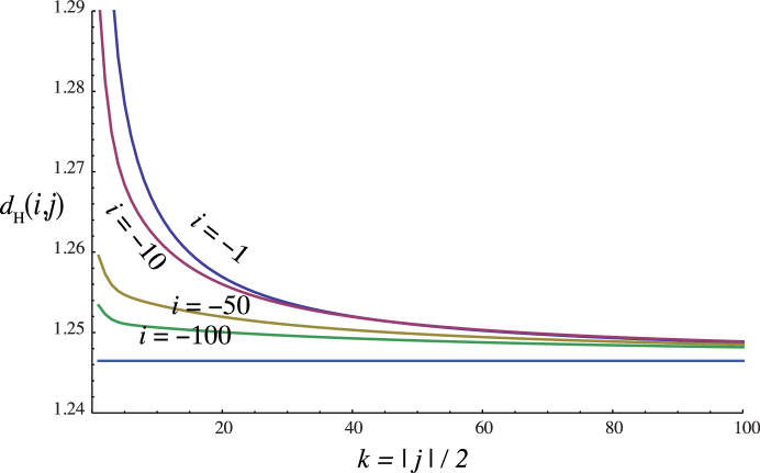
Figure 27: Plots of $d_{H}(i,j)$ versus $k=|j|/2$ for $i=-1$ (top curve),$-10,-50,$ and $-100$ and $2\leqslant k\leqslant 100$. Calculated points have been joined by straight segments to aid the eye. The horizontal asymptote corresponds to the value $d_{\infty}$.

Appendix A: Catalogue of polygonal shapes

Table 5: Polygonal shapes encountered in the text. All of these are convex with the exception of $\widehat{\mathrm{A}}$, the arrowhead.

$$\begin{array}[]{|c|c|}\hline\cr Q_{1}(l)&[(6,1,3),(l,0,0)]\\ \hline\cr Q_{2}(l)&[(4,6,0,2),(l,l,l,l)]\\ \hline\cr Q_{3}(l)&[(6,7,2,3),(l,l,l,l)]\\ \hline\cr Q_{4}(l_{1},l_{2})&[(6,1,2,3),(l_{1},0,-l_{2},0)]\\ \hline\cr Q_{5}(l)&[(0,1,\ldots,7),(l,l,\ldots,l)]\\ \hline\cr Q_{6}(l_{1},l_{2})&[(5,6,0,2,3),(0,l_{2},l_{1},l_{2},0)]\\ \hline\cr Q_{7}(l)&[(5,7,0,2),(0,l,l,0)]\\ \hline\cr Q_{8}(l_{1},l_{2})&[(4,5,7,0,1,2),(0,0,l_{1},l_{2},l_{2},l_{1})]\\ \hline\cr Q_{9}(l_{1},l_{2})&[(1,2,3,5,6,7),(l_{1},l_{2},l_{1},l_{1},l_{2},l_{1})]\\ \hline\cr Q_{10}(l_{1},l_{2})&[(4,6,0,2),(l_{2},l_{1},l_{2},l_{1})]\\ \hline\cr Q_{11}(l_{1},l_{2},l_{3})&[(1,2,3,5,6,7),(l_{1},l_{2},l_{1},l_{1},l_{2},l_{1})]\\ \hline\cr Q_{12}(l_{1},l_{2})&[(6,0,2,3),(0,l_{1},l_{2},0)]\\ \hline\cr Q_{13}(l_{1},l_{2})&[(5,6,0,2),(0,l_{2},l_{1},0)]\\ \hline\cr Q_{14}(l_{1},l_{2})&[(0,1,\ldots,7),(l_{1},l_{1},l_{2},l_{2},l_{1},l_{1},l_{2},l_{2})]\\ \hline\cr Q_{15}(l_{1},l_{2})&[(0,1,\ldots,7),(l_{1},l_{2},l_{1},l_{2},l_{1},l_{2},l_{1},l_{2})]\\ \hline\cr\widehat{\mathrm{A}}(l)&[(5,0,2),(l,l,0)]\cup[(5,0,3),(l,l,0)]\\ \hline\cr\end{array}$$

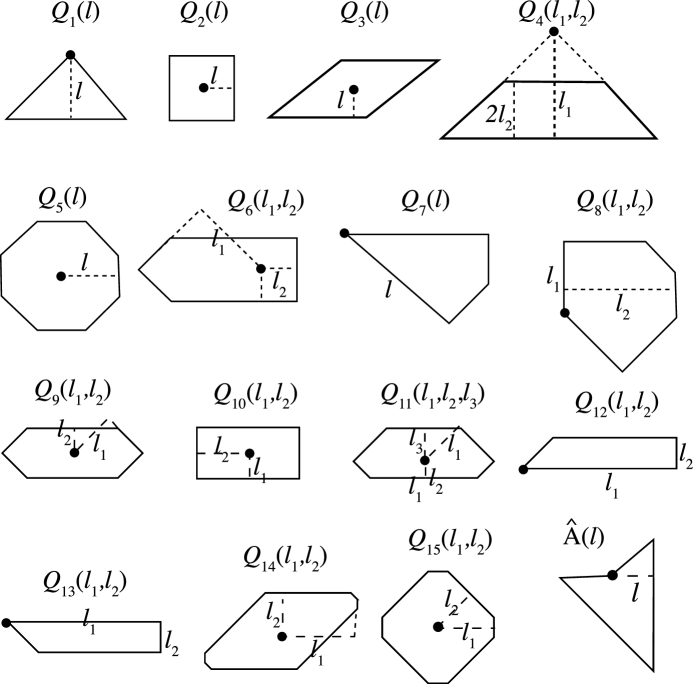
Figure 28: Polygonal shapes listed in Table 5, with anchor points emphasized.

Appendix B: Tiling plans

Key:

• Heading, ‘Parent dressed domain’:    PWI for constructing orbits by direct iteration.

• Heading, ‘Tiling domains’:   spans of listed source tiles, expressed in terms of the representative polygons of Appendix A.

• Col. 1, ‘Tile’:   name of source tile whose orbit is to be calculated.

• Cols 2, 3, ‘$Q_{\#}$’, ‘Parameters’:   source tile representative polygon and parameters (see Appendix A).

• Cols 4, 5, ‘$\mathtt{R}_{\#}$’, ‘Translation’:  index $n$ of rotation $\mathtt{R}_{n}$, and translation $(d_{x},d_{y})$ of source tile relative to representative polygon.

• Col 6, 7: ‘tile’, ‘$\mathtt{R}_{\#}$’:   destination tile and index $n$ of net rotation $\mathtt{R}_{n}$ relative to source tile. These specify the net isometry to be verified by direct iteration.

$$\begin{array}[]{|c|}\hline\cr\\ \mbox{TILING PLAN 1 :}\quad{\mathcal{B}}\rightarrow{\mathcal{B}}^{*},\quad s\in I_{0,-1}=(\beta+\beta^{3},\alpha\beta)\\ \\ \hline\cr\begin{array}[]{l}\\ \mbox{Parent dressed domain:}\qquad\widehat{{\mathcal{B}}}(1,s)\\ \\ \mbox{Tiling domain:}\quad{\rm B}^{*}={\tt T}_{(-2\beta^{2}+\beta s,-4\beta-s)}\,\,{\tt R}_{2}\,\,Q_{1}(2\beta^{2}-\beta s)\\ \end{array}\\ \\ \mbox{\sc Data for Direct Iteration}\\ \begin{array}[]{c|c|c|c|c|c|c}\hline\cr\lx@intercol\hfil\mbox{Source Polygon}\hfil\lx@intercol\vrule\lx@intercol&\vrule\lx@intercol\hfil\mbox{Initial Placement}\hfil\lx@intercol\vrule\lx@intercol&\vrule\lx@intercol\hfil\mbox{Destination}\hfil\lx@intercol\\ \hline\cr\mbox{Tile}&Q_{\#}&\mbox{Parameters}&{\tt R}_{\#}&\mbox{Translation}&\mbox{Tile}&{\tt R}_{\#}\\ \hline\cr\hline\cr B^{*}_{1}&1&-2\alpha\beta^{3}+\beta s&7&(0,-2-4\beta^{3})&B^{*}_{1}\oslash B^{*}&6\\ \hline\cr B^{*}_{2}&7&-4\beta^{2}+\alpha s&6&(0,14-12\alpha+\alpha s)&B^{*}_{2}\oslash B^{*}&5\\ \hline\cr B^{*}_{3}&6&-\alpha\beta^{3}+\beta s,\alpha\beta-\ s&5&(0,12-10\alpha)&B^{*}_{3}\oslash B^{*}&6\\ \hline\cr B^{*}_{4}&7&2\beta-\alpha s&1&(-2\beta+\alpha s,12-10\alpha)&B^{*}_{4}\oslash B^{*}&7\\ \hline\cr B^{*}_{5}&1&\alpha\beta^{2}-\beta s&2&(-\alpha\beta^{2}+\beta s,14-11\alpha-s)&B^{*}_{5}\oslash B^{*}&0\\ \hline\cr\hline\cr\Pi_{1}&2&s&0&(-s,-s)&\Pi_{1}&2\\ \hline\cr\Pi_{2}&5&2\beta-\ s&0&(-2\beta-s,-s)&\Pi_{2}&5\\ \hline\cr\Pi_{3}&3&-\beta+s&0&(-1-s,\beta-s)&\Pi_{3}&4\\ \hline\cr\Pi_{4}&5&\alpha\beta-s&0&(-\alpha\beta-s,-\alpha\beta-s)&\Pi_{4}&3\\ \hline\cr\Pi_{5}&5&\alpha\beta-s&0&(\alpha\beta^{2}-s,-\alpha-s)&\Pi_{5}&3\\ \hline\cr\Pi_{6}&7&2\beta-\alpha s&5&(4\beta-(2+\alpha)s,-2\beta-2s)&\Pi_{6}&0\\ \hline\cr\Pi_{7}&1&\alpha\beta^{2}-\beta s&6&(-6+5\alpha-\omega s,-\alpha-s)&\Pi_{7}&0\\ \hline\cr\Pi_{8}&5&-2\alpha\beta^{2}+s&0&(2\alpha\beta^{2}-s,10-8\alpha-s)&\Pi_{8}&3\\ \hline\cr\Pi_{9}&10&\alpha\beta-s,-2\alpha\beta^{2}+s&1&(\beta-s,-3\beta-s)&\Pi_{9}&4\\ \end{array}\\ \hline\cr\end{array}$$

$$\begin{array}[]{|c|}\hline\cr\\ \mbox{TILING PLAN 2 :}\quad{\mathcal{B}}\rightarrow{\mathcal{B}}^{*},\quad s=\beta\\ \\ \hline\cr\begin{array}[]{l}\\ \mbox{Parent dressed domain:}\qquad\widehat{{\mathcal{B}}}(1,s)\\ \\ \mbox{Tiling domains:}\quad\begin{array}[]{l}{\rm B}^{*}={\tt T}_{(-\beta,1-2\alpha)}\,\,{\tt R}_{2}\,\,Q_{1}(\beta)\\ {\rm B}^{\dagger}={\tt T}_{(-4\beta,-2\alpha\beta^{2})}\,\,{\tt R}_{7}\,\,{Q}_{1}(\beta^{3})\end{array}\end{array}\\ \\ \mbox{\sc Data for Direct Iteration}\\ \begin{array}[]{c|c|c|c|c|c|c}\hline\cr\lx@intercol\hfil\mbox{Source Polygon}\hfil\lx@intercol\vrule\lx@intercol&\vrule\lx@intercol\hfil\mbox{Initial Placement}\hfil\lx@intercol\vrule\lx@intercol&\vrule\lx@intercol\hfil\mbox{Destination}\hfil\lx@intercol\\ \hline\cr\mbox{Tile}&Q_{\#}&\mbox{Parameters}&{\tt R}_{\#}&\mbox{Translation}&\mbox{Tile}&{\tt R}_{\#}\\ \hline\cr\hline\cr B^{*}_{1}&1&\beta^{2}&5&(0,-4\beta)&B^{*}_{1}\oslash B^{*}&2\\ \hline\cr B^{*}_{2}&7&\alpha\beta&3&(0,2-3\alpha)&B^{*}_{2}\oslash B^{*}&3\\ \hline\cr B^{\dagger}_{1}&1&\beta^{4}&2&(-13+8\alpha,15-11\alpha)&B^{\dagger}_{1}\oslash B^{\dagger}&2\\ \hline\cr B^{\dagger}_{2}&7&\alpha\beta^{3}&0&(-3\alpha\beta,-2\alpha\beta^{2})&B^{\dagger}_{2}\oslash B^{\dagger}&3\\ \hline\cr\hline\cr\Pi_{1}&2&\beta&0&\left(-\beta,-\beta\right)&\Pi_{1}&2\\ \hline\cr\Pi_{2}&5&\beta&0&(-3\beta,-\beta&\Pi_{2}&5\\ \hline\cr\Pi_{3}&5&\beta^{3}&0&(11-9\alpha,-\beta)&\Pi_{3}&5\\ \hline\cr\Pi_{4}&5&\beta^{2}&0&(-1,-1)&\Pi_{4}&3\end{array}\\ \hline\cr\end{array}$$

$$\begin{array}[]{|c|}\hline\cr\\ \mbox{TILING PLAN 3 :}\quad{\mathcal{B}}\rightarrow{\mathcal{P}},\quad s\in(0,\alpha\beta^{2})\\ \\ \hline\cr\begin{array}[]{l}\\ \mbox{Parent dressed domain:}\qquad\widehat{{\mathcal{B}}}(1,s)\\ \\ \mbox{Tiling domains:}\quad\begin{array}[]{l}{\rm P}={\tt T}_{(-2+\beta s,-s)}\,\,{Q}_{6}(2-\beta s,s)\\ {\rm A}={\tt T}_{(-2\beta^{2}-\alpha\beta s,-2\alpha\beta-2s)}\,\,\widehat{\rm A}(2\beta^{2}-\alpha s)\end{array}\par\end{array}\\ \\ \mbox{\sc Data for Direct Iteration}\\ \begin{array}[]{c|c|c|c|c|c|c}\hline\cr\lx@intercol\hfil\mbox{Source Polygon}\hfil\lx@intercol\vrule\lx@intercol&\vrule\lx@intercol\hfil\mbox{Initial Placement}\hfil\lx@intercol\vrule\lx@intercol&\vrule\lx@intercol\hfil\mbox{Destination}\hfil\lx@intercol\\ \hline\cr\mbox{Tile}&Q_{\#}&\mbox{Parameters}&{\tt R}_{\#}&\mbox{Translation}&\mbox{Tile}&{\tt R}_{\#}\\ \hline\cr\hline\cr P_{0}&2&s&0&(-s,-s)&P_{0}\oslash P&2\\ \hline\cr P_{1}&9&\beta-s,s&0&(-\alpha-s,-s)&P_{1}\oslash P&4\\ \hline\cr P_{2}&7&\alpha s&1&(-2\beta-\alpha\omega s,-2s)&P_{2}\oslash P&7\\ \hline\cr P_{3}&1&\beta s&3&(-2\beta-2s,-2s)&P_{5}\oslash P&6\\ \hline\cr P_{4}&3&s&3&(-2\beta-s,-s)&P_{4}\oslash P&5\\ \hline\cr P_{5}&4&\alpha\beta^{2}-\beta s,\alpha\beta^{2}-\omega s&4&(-\alpha\beta-s,-\alpha\beta^{2}+\beta s)&P_{3}\oslash P&4\\ \hline\cr P_{6}&3&s&0&(-2\beta^{2}-s,-s)&P_{6}\oslash P&3\\ \hline\cr P_{\rm in}&12&2\beta^{2}-\alpha\ s,2s&0&(-2\beta^{2}-\alpha\beta s,-2s)&A_{2}\oslash{\rm A}&0\\ \hline\cr\hline\cr A_{1}&1&\alpha\beta-\omega s&2&(-\alpha\beta+\beta s,-\alpha-s)&A_{1}\oslash{\rm A}&5\\ \hline\cr A_{2}&13&2\beta^{2}-\alpha s,2s&5&(-2\beta^{2}-\alpha\beta s,-2\alpha\beta-2s)&P_{\rm in}\oslash P&3\\ \hline\cr A_{3}&1&\alpha\beta^{2}-\omega s&4&(-\alpha\beta-s,-\alpha+\beta s)&A_{3}\oslash{\rm A}&1\\ \hline\cr\hline\cr\Pi&5&\alpha\beta-s&0&(-\alpha\beta-s,-\alpha\beta-s)&\Pi&3\end{array}\\ \hline\cr\end{array}$$

$$\begin{array}[]{|c|}\hline\cr\\ \mbox{TILING PLAN 4 : }\quad{\mathcal{P}}\rightarrow{\mathcal{B}},\quad s=\beta^{2}\\ \\ \hline\cr\\ \mbox{Parent dressed domain:}\qquad\widehat{{\mathcal{P}}}(\alpha,\beta^{2})\\ \\ \mbox{Tiling domains:}\quad\begin{array}[]{l}{\rm B}^{*}={\tt T}_{(-\alpha\beta,0)}{\tt R}_{4}Q_{1}(\beta^{2})\\ {\rm B}^{\dagger}={\tt T}_{(-\alpha\beta^{2},-2\beta^{3})}Q_{1}(\beta^{5})\end{array}\\ \\ \mbox{\sc Data for Direct Iteration}\\ \begin{array}[]{c|c|c|c|c|c|c}\hline\cr\lx@intercol\hfil\mbox{Source Polygon}\hfil\lx@intercol\vrule\lx@intercol&\vrule\lx@intercol\hfil\mbox{Initial Placement}\hfil\lx@intercol\vrule\lx@intercol&\vrule\lx@intercol\hfil\mbox{Destination}\hfil\lx@intercol\\ \hline\cr\mbox{Tile}&Q_{\#}&\mbox{Parameters}&{\tt R}_{\#}&\mbox{Translation}&\mbox{Tile}&{\tt R}_{\#}\\ \hline\cr\hline\cr B^{*}_{1}&1&\beta^{3}&1&(-3\beta^{2},\beta^{2})&B^{*}_{1}\oslash B^{*}&6\\ \hline\cr B^{*}_{2}&7&\alpha\beta^{2}&0&(-5+3\alpha,\beta^{2})&B^{*}_{2}\oslash B^{*}&5\\ \hline\cr B^{\dagger}_{1}&1&\beta^{5}&5&(-\beta^{5}-\alpha\beta^{2},-\beta^{2})&B^{\dagger}_{1}\oslash B^{\dagger}&6\\ \hline\cr B^{\dagger}_{2}&7&\alpha\beta^{4}&4&(-3\beta^{3},-\beta^{2})&B^{\dagger}_{2}\oslash B^{\dagger}&5\\ \hline\cr\Pi_{1}&2&\beta^{2}&0&(0,0)&\Pi_{1}&2\\ \hline\cr\Pi_{2}&9&\alpha\beta^{2},\beta^{2}&0&(-\alpha,0))&\Pi_{2}&4\\ \hline\cr\Pi_{3}&1&\beta^{3}&3&(-1,-\beta^{2})&\Pi_{3}&0\\ \hline\cr\Pi_{4}&5&\beta^{2}&0&(-2\beta,0)&\Pi_{4}&5\\ \hline\cr\Pi_{5}&5&\beta^{2}&0&(-2\beta^{2},0)&\Pi_{5}&3\\ \hline\cr\Pi_{6}&5&\beta^{4}&0&(\alpha\beta^{4}-\alpha\beta,0)&\Pi_{6}&3\end{array}\\ \hline\cr\end{array}$$

$$\begin{array}[]{|c|}\hline\cr\\ \mbox{TILING PLAN 5 :}\quad{\mathcal{B}}\rightarrow{\mathcal{T}}_{-},\quad s\in(\beta,\beta+\beta^{4}]\\ \\ \hline\cr\begin{array}[]{l}\\ \mbox{Parent dressed domain:}\qquad\widehat{{\mathcal{B}}}(1,s)\\ \\ \mbox{Tiling domains:}\quad\begin{array}[]{l}\mathrm{T}_{-}={\tt T}_{(-\alpha\beta+\beta s,-\alpha-s)}{\tt R}_{2}Q_{1}(\alpha\beta-\beta s)\\ \mathrm{A}={\tt T}_{(-2\beta-\alpha\beta s,-2s)}\widehat{A}(2\beta-\alpha s)\end{array}\end{array}\\ \\ \mbox{\sc Data for Direct Iteration}\\ \begin{array}[]{c|c|c|c|c|c|c}\hline\cr\lx@intercol\hfil\mbox{Source Polygon}\hfil\lx@intercol\vrule\lx@intercol&\vrule\lx@intercol\hfil\mbox{Initial Placement}\hfil\lx@intercol\vrule\lx@intercol&\vrule\lx@intercol\hfil\mbox{Destination}\hfil\lx@intercol\\ \hline\cr\mbox{Tile}&Q_{\#}&\mbox{Parameters}&{\tt R}_{\#}&\mbox{Translation}&\mbox{Tile}&{\tt R}_{\#}\\ \hline\cr\hline\cr T^{-}_{1}&1&\beta s&5&(0,-2\beta-2s)&T^{-}_{1}\oslash{\rm T}_{-}&2\\ \hline\cr T^{-}_{2}&7&2-\omega s&3&(2\beta-2s,-2\alpha+\alpha s)&T^{-}_{2}\oslash{\rm T}_{-}&3\\ \hline\cr T^{-}_{3}&3&-\beta+s&1&(\beta-s,7-6\alpha-s)&T^{-}_{3}\oslash{\rm T}_{-}&1\\ \hline\cr T^{-}_{4}&4&2\beta^{2}-\beta s,2\alpha\beta-\omega s&2&(-2\beta^{2}+\beta s,-4\beta-s)&T^{-}_{4}\oslash{\rm T}_{-}&0\\ \hline\cr T^{-}_{{\rm in}}&13&2\beta-\alpha s,-2\beta+2s&2&(2\beta-2s,-4\beta-\alpha\beta s)&A_{2}\oslash\mathrm{A}&3\\ \hline\cr A_{1}&1&\alpha-\omega s&7&(-2s,-2s)&A_{1}\oslash\mathrm{A}&3\\ \hline\cr A_{2}&12&2\beta-\alpha s,-2\beta+2s&0&(-2\beta-\alpha\beta s,-2s)&T^{-}_{{\rm in}}\oslash\mathrm{T}_{-}&6\\ \hline\cr A_{3}&1&2\alpha\beta-\omega s&5&(-2s,-2\beta)&\widehat{A}_{3}\oslash\mathrm{A}&7\\ \hline\cr\Pi_{1}&2&s&0&(-s,-s)&\Pi_{1}&2\\ \hline\cr\Pi_{2}&5&2\beta-s&0&(-2\beta-s,-s)&\Pi_{2}&5\\ \hline\cr\Pi_{3}&3&-\beta+s&0&(-1-s,\beta-s)&\Pi_{3}&4\end{array}\\ \hline\cr\end{array}$$

$$\begin{array}[]{|c|}\hline\cr\\ \mbox{TILING PLAN 6 :}\quad{\mathcal{B}}\rightarrow{\mathcal{T}}_{+},\quad s\in[\beta-\beta^{6},\beta)\\ \\ \hline\cr\begin{array}[]{l}\\ \mbox{Parent dressed domain:}\qquad\widehat{{\mathcal{B}}}(1,s)\\ \\ \mbox{Tiling domains:}\quad\begin{array}[]{l}\mathrm{T}_{+}={\tt T}_{(-\alpha\beta+\beta s,-\alpha-s)}{\tt R}_{2}Q_{1}(\alpha\beta-\beta s)\\ \mathrm{A}={\tt T}_{(-2\beta^{2}-\alpha s,-2s)}{\tt R}_{3}\widehat{A}(-2\alpha\beta^{2}+\alpha s)\end{array}\end{array}\\ \\ \mbox{\sc Data for Direct Iteration}\\ \begin{array}[]{c|c|c|c|c|c|c}\hline\cr\lx@intercol\hfil\mbox{Source Polygon}\hfil\lx@intercol\vrule\lx@intercol&\vrule\lx@intercol\hfil\mbox{Initial Placement}\hfil\lx@intercol\vrule\lx@intercol&\vrule\lx@intercol\hfil\mbox{Destination}\hfil\lx@intercol\\ \hline\cr\mbox{Tile}&Q_{\#}&\mbox{Parameters}&{\tt R}_{\#}&\mbox{Translation}&\mbox{Tile}&{\tt R}_{\#}\\ \hline\cr\hline\cr T^{+}_{1}&1&\beta s&5&(0,-2\beta-2s)&T^{+}_{1}\oslash\mathrm{T}_{+}&2\\ \hline\cr T^{+}_{2}&7&\alpha s&3&(0,-2\beta-\alpha\omega s)&T^{+}_{2}\oslash\mathrm{T}_{+}&3\\ \hline\cr T^{+}_{3}&4&\beta s,-2\beta+\omega s&7&(0,-2)&T^{+}_{3}\oslash\mathrm{T}_{+}&6\\ \hline\cr T^{+}_{4}&3&\beta-s&7&\beta^{2}-s,-3+\alpha-s)&T^{+}_{4}\oslash\mathrm{T}_{+}&1\\ \hline\cr T^{+}_{5}&2&\beta-s&1&(\alpha\beta^{3}-s,-10+6\alpha-s)&T^{+}_{5}\oslash\mathrm{T}_{+}&4\\ \hline\cr T^{+}_{6}&10&\beta-s,-2\beta^{2}+s&7&(\alpha\beta^{3}/2-s,-5\alpha\beta/2-s)&T^{+}_{6}\oslash{\rm T}_{+}&6\\ \hline\cr T^{+}_{7}&2&\beta-s&1&(-s,-\alpha-s)&T^{+}_{7}\oslash\mathrm{T}_{+}&4\\ \hline\cr T^{+}_{\rm in}&12&-2\alpha\beta^{2}+\alpha s,2\beta-2s&3&(2\beta^{2}-\alpha s,-2\alpha\beta-2s)&A_{2}\oslash\mathrm{A}&0\\ \hline\cr A_{1}&1&-2\beta+\omega s&5&(-2\beta,-2s)&A_{1}\oslash{\rm A}&5\\ \hline\cr A_{2}&13&-2\alpha\beta^{2}+\alpha s,2\beta-2s&0&(-2\beta^{2}-\alpha s,-2s)&T^{+}_{\rm in}\oslash\mathrm{T}_{+}&5\\ \hline\cr A_{3}&1&\beta^{3}-1+\omega s&7&(-2\beta,-2\beta)&A_{3}\oslash{\rm A}&1\\ \hline\cr\Pi_{1}&2&s&0&(-s,-s)&\Pi_{1}&2\\ \hline\cr\Pi_{2}&5&s&0&(-2\beta-s,-s)&\Pi_{2}&5\\ \hline\cr\Pi_{3}&5&\alpha\beta-s&0&(-\alpha\beta-s,-\alpha\beta-s)&\Pi_{3}&3\end{array}\\ \hline\cr\end{array}$$

$$\begin{array}[]{|c|}\hline\cr\\ \mbox{TILING PLAN 7 :}\quad{\mathcal{P}}^{*}\rightarrow{\mathcal{T}}_{-},\quad s\in(\beta^{2},\beta^{2}+\beta^{6}]\\ \\ \hline\cr\begin{array}[]{l}\\ \mbox{Parent dressed domain:}\qquad\widehat{{\mathcal{P}}}(\alpha,s)\\ \\ \mbox{Tiling domains:}\quad\begin{array}[]{l}\mathrm{T}_{-}={\tt T}_{(-\alpha\beta,-\alpha\beta^{2}+\alpha s)}{\tt R}_{4}Q_{1}(\alpha\beta^{2}-\beta s)\\ \mathrm{A}={\tt T}_{(-2\beta^{4}-s,-2\alpha\beta^{4}-\beta s)}{\tt R}_{6}\widehat{A}(\alpha\beta^{5}+\alpha\beta^{2}-\alpha s)\end{array}\end{array}\\ \\ \mbox{\sc Data for Direct Iteration}\\ \begin{array}[]{c|c|c|c|c|c|c}\hline\cr\lx@intercol\hfil\mbox{Source Polygon}\hfil\lx@intercol\vrule\lx@intercol&\vrule\lx@intercol\hfil\mbox{Initial Placement}\hfil\lx@intercol\vrule\lx@intercol&\vrule\lx@intercol\hfil\mbox{Destination}\hfil\lx@intercol\\ \hline\cr\mbox{Tile}&Q_{\#}&\mbox{Parameters}&{\tt R}_{\#}&\mbox{Translation}&\mbox{Tile}&{\tt R}_{\#}\\ \hline\cr\hline\cr T^{-}_{1}&1&\beta s&1&(-2\beta^{2}-s,s)&T^{-}_{1}\oslash{\rm T}_{-}&6\\ \hline\cr T^{-}_{2}&7&2\beta-\alpha\omega s&0&(-2\alpha\beta+\omega s,2\beta^{2}-s)&T^{-}_{2}\oslash{\rm T}_{-}&5\\ \hline\cr T^{-}_{3}&4&2\beta^{3}-\beta s&4&(-3\beta^{2},-2\beta^{3}+\alpha s)&T^{-}_{3}\oslash{\rm T}_{-}&0\\ \hline\cr T^{-}_{4}&3&-\beta^{2}+s&0&(-\beta^{4}-\alpha\beta,\beta^{2})&T^{-}_{4}\oslash{\rm T}_{-}&7\\ \hline\cr T^{-}_{5}&4&\begin{array}[]{c}\alpha\beta^{3}-\beta s,\\ \beta^{4}+\beta-\omega s\end{array}&0&(-\alpha\beta,\beta^{4}+\beta-\alpha s)&T^{-}_{5}\oslash{\rm T}_{-}&0\\ \hline\cr T^{-}_{6}&3&-\beta^{2}+s&7&(\beta^{4}+\alpha\beta,\beta^{2})&T^{-}_{6}\oslash{\rm T}_{-}&1\\ \hline\cr T^{-}_{7}&4&\begin{array}[]{c}2\alpha\beta^{4}-\beta s,\\ \beta^{5}+\beta-\omega s\end{array}&4&(\alpha\beta^{4}+\beta,-2\alpha\beta^{4}+\alpha s)&T^{-}_{7}\oslash{\rm T}_{-}&0\\ \hline\cr T^{-}_{8}&3&-\beta^{2}+s&0&(-4\beta^{4}-\beta,\beta^{2})&T^{-}_{8}\oslash{\rm T}_{-}&7\\ \hline\cr T^{-}_{\rm in}&12&\begin{array}[]{c}\alpha\beta^{5}+\alpha\beta^{2}-\alpha s,\\ -2\beta^{2}+2s\end{array}&0&(-\beta^{5}+\beta+\beta s,2\beta^{2}-s)&A_{2}\oslash{\rm A}&6\\ \hline\cr A_{1}&1&\beta^{4}+\beta-\omega s&0&(-\alpha\beta^{2},\alpha\beta^{3}-\alpha s)&A_{1}\oslash{\rm A}&5\\ \hline\cr A_{2}&13&\begin{array}[]{c}\alpha\beta^{5}+\alpha\beta^{2}-\alpha s,\\ -2\beta^{2}+2s\end{array}&3&(-2\beta^{4}-s,-2\alpha\beta^{4}-\beta s)&T^{-}_{\rm in}\oslash{\rm T}_{-}&1\\ \hline\cr A_{3}&1&\beta^{5}+\beta-\omega s&2&(-2\alpha\beta^{2}+\alpha s,-2\beta^{3})&A_{3}\oslash{\rm A}&1\\ \hline\cr\Pi_{1}&2&s&0&(0,0)&\Pi_{1}&2\\ \hline\cr\Pi_{2}&3&-\beta^{2}+s&7&(-3\beta,\beta^{2})&\Pi_{2}&4\\ \hline\cr\Pi_{3}&9&\beta-s,s&0&(-\alpha,0)&\Pi_{3}&4\\ \hline\cr\Pi_{4}&1&\beta s&3&(-2\beta-s,-s)&\Pi_{4}&0\\ \hline\cr\Pi_{5}&5&2\beta^{2}-s&0&(-2\beta^{2},0)&\Pi_{5}&3\\ \hline\cr\Pi_{6}&5&s&0&(-2\beta-s,-s)&\Pi_{6}&5\\ \hline\cr\Pi_{7}&5&2\alpha\beta^{3}-s&0&(-2\alpha\beta^{3},-2\beta^{3})&\Pi_{7}&3\\ \hline\cr\end{array}\\ \hline\cr\end{array}$$

$$\begin{array}[]{|c|}\hline\cr\\ \mbox{TILING PLAN 8 :}\quad{\mathcal{P}}^{*}\rightarrow{\mathcal{T}}_{+},\quad s\in[\beta^{2}-\beta^{7},\beta^{2})\\ \\ \hline\cr\begin{array}[]{l}\\ \mbox{Parent dressed domain:}\qquad\widehat{{\mathcal{P}}}(\alpha,s)\\ \\ \mbox{Tiling domains:}\quad\begin{array}[]{l}{\rm T}_{+}={\tt T}_{(-\alpha\beta,-\alpha\beta^{2}+\alpha s)}{\tt R}_{4}Q_{1}(\alpha\beta^{2}-\beta s)\\ {\rm A}={\tt T}_{(-4\alpha\beta^{2}+s,\alpha\beta^{5}-\alpha\beta^{2}+\beta s)}{\tt R}_{6}\widehat{A}(\alpha\beta^{5}-\alpha\beta^{2}+\alpha s)\end{array}\end{array}\\ \\ \mbox{\sc Data for Direct Iteration}\\ \begin{array}[]{c|c|c|c|c|c|c}\hline\cr\lx@intercol\hfil\mbox{Source Polygon}\hfil\lx@intercol\vrule\lx@intercol&\vrule\lx@intercol\hfil\mbox{Initial Placement}\hfil\lx@intercol\vrule\lx@intercol&\vrule\lx@intercol\hfil\mbox{Destination}\hfil\lx@intercol\\ \hline\cr\mbox{Tile}&Q_{\#}&\mbox{Parameters}&{\tt R}_{\#}&\mbox{Translation}&\mbox{Tile}&{\tt R}_{\#}\\ \hline\cr\hline\cr T^{+}_{1}&1&\beta s&1&(-2\beta^{2}-s,s)&T^{+}_{1}\oslash{\rm T}_{+}&6\\ \hline\cr T^{+}_{2}&7&\alpha s&0&(-2\beta^{2}-\omega s,s)&T^{+}_{2}\oslash{\rm T}_{+}&5\\ \hline\cr T^{+}_{3}&4&\beta s,-2\beta^{2}+s&7&(-2\beta+s,s)&T^{+}_{3}\oslash{\rm T}_{+}&2\\ \hline\cr T^{+}_{4}&3&\beta^{2}-s&2&(2\beta^{2}-1,\beta^{3})&T^{+}_{4}\oslash{\rm T}_{+}&7\\ \hline\cr T^{+}_{5}&2&\beta^{2}-s&1&(-3\beta^{3}-\beta,\alpha\beta^{4})&T^{+}_{5}\oslash{\rm T}_{+}&4\\ T^{+}_{6}&10&-2\beta^{3}+s,\beta^{2}-s&1&(-5\alpha\beta^{2}/2,\alpha\beta^{4}/2)&T^{+}_{6}\oslash{\rm T}_{+}&2\\ \hline\cr T^{+}_{7}&2&\beta^{2}-s&1&(-\alpha\beta,0)&T^{+}_{7}\oslash{\rm T}_{+}&4\\ \hline\cr T^{+}_{8}&4&\begin{array}[]{c}-2\beta^{4}+\beta s,\\ -4\alpha\beta^{3}+s\end{array}&3&\begin{array}[]{c}(-2\alpha\beta^{2}-s,\\ 9\beta^{3}-\beta-s)\end{array}&T^{+}_{8}\oslash{\rm T}_{+}&2\\ \hline\cr T^{+}_{9}&3&\beta^{2}-s&7&(-9\beta^{3},9\beta^{3}-\alpha\beta)&T^{+}_{9}\oslash{\rm T}_{+}&1\\ \hline\cr T^{+}_{\rm in}&12&\begin{array}[]{c}-9\beta^{3}+\beta+\alpha s,\\ 2\beta^{2}-2s\end{array}&7&\begin{array}[]{c}(-10\beta^{3}+\beta s,\\ -4\beta^{4}+s)\end{array}&A_{2}\oslash{\rm A}&7\\ \hline\cr A_{1}&1&\beta^{4}-\beta+s&0&(-\alpha\beta^{2},\beta^{4}-\beta+\alpha s)&A_{1}\oslash{\rm A}&5\\ \hline\cr A_{2}&13&\begin{array}[]{c}-9\beta^{3}+\beta+\alpha s,\\ 2\beta^{2}-2s\end{array}&3&\begin{array}[]{c}(-4\alpha\beta^{3}+s,\\ -9\beta^{4}+\beta+\beta s)\end{array}&T^{+}_{\rm in}\oslash{\rm T}_{+}&2\\ \hline\cr A_{3}&1&-4\alpha\beta^{3}+\omega s&2&(-\alpha s,-2\beta^{3})&A_{3}\oslash{\rm A}&1\\ \hline\cr\Pi_{1}&2&s&0&(0,0)&\Pi_{1}&2\\ \hline\cr\Pi_{2}&9&\beta-s,\beta s&0&(-\alpha,0)&\Pi_{2}&4\\ \hline\cr\Pi_{3}&1&\beta s&3&(-2\beta-s,-s)&\Pi_{3}&0\\ \hline\cr\Pi_{4}&5&s&0&(-2\beta^{2},0)&\Pi_{4}&3\\ \hline\cr\Pi_{5}&5&s&0&(-2\beta,0)&\Pi_{5}&5\\ \hline\cr\Pi_{6}&5&-2\beta^{3}+s&0&(-2\alpha\beta^{3},-2\beta^{3})&\Pi_{6}&3\end{array}\\ \hline\cr\end{array}$$

$$\begin{array}[]{|c|}\hline\cr\\ \mbox{TILING PLAN 9 :}\quad{\mathcal{T}}_{-}\rightarrow{\mathcal{D}}_{-},\quad s-\beta\in(0,\beta^{4}]\\ \\ \hline\cr\begin{array}[]{l}\\ \mbox{Parent dressed domain:}\qquad\widehat{{\mathcal{T}}}_{-}(\beta,h),\quad h=s-\beta\\ \\ \mbox{Tiling domains:}\quad\begin{array}[]{l}{\rm D}={\tt T}_{(-\beta^{2}+\alpha h,-\beta+h)}{\tt R}_{2}Q_{4}(\beta^{2}-\beta h,\beta^{2}-\omega h)\\ {\rm X}={\tt T}_{(h,-\alpha\beta^{3}+\alpha h)}{\tt R}_{2}Q_{12}(\alpha\beta^{3}-\alpha h,2h)\\ {\rm A}={\tt T}_{(-\alpha\beta^{3}+\beta h,2h)}{\tt R}_{3}\widehat{A}(\alpha\beta^{3}-\alpha h)\end{array}\end{array}\\ \\ \mbox{\sc Data for Direct Iteration}\\ \begin{array}[]{c|c|c|c|c|c|c}\hline\cr\lx@intercol\hfil\mbox{Source Polygon}\hfil\lx@intercol\vrule\lx@intercol&\vrule\lx@intercol\hfil\mbox{Initial Placement}\hfil\lx@intercol\vrule\lx@intercol&\vrule\lx@intercol\hfil\mbox{Destination}\hfil\lx@intercol\\ \hline\cr\mbox{Tile}&Q_{\#}&\mbox{Parameters}&{\tt R}_{\#}&\mbox{Translation}&\mbox{Tile}&{\tt R}_{\#}\\ \hline\cr\hline\cr D_{1}^{\prime\prime}&4&\beta^{3}-\beta h,\beta^{3}-\omega h&2&(-\beta^{3}+\alpha h,11-8\alpha+h)&D_{1}^{\prime\prime}\oslash{\rm D}&0\\ \hline\cr D_{2}^{\prime\prime}&3&h&2&(0,18-13\alpha+h)&D_{2}^{\prime\prime}\oslash{\rm D}&7\\ \hline\cr D_{\rm in}^{\prime\prime}&12&\alpha\beta^{3}-\alpha h,2h&6&(-h,18-13\alpha+\alpha\beta h)&A_{2}\oslash{\rm A}&5\\ \hline\cr D_{0}&2&h&0&(0,-2\alpha\beta^{2}+h)&D_{0}\oslash{\rm D}&2\\ \hline\cr D_{1}^{\prime}&12&\alpha\beta^{3}-\alpha h,2h&2&(\alpha\beta^{3}-\alpha h,2h)&X&0\\ \hline\cr A_{1}&1&\beta^{2}-\omega h&5&(-h,2h)&A_{1}\oslash{\rm A}&5\\ \hline\cr A_{2}&13&\alpha\beta^{3}-\alpha h,2h&0&(-\alpha\beta^{3}+\beta h)&D_{\rm in}^{\prime\prime}\oslash{\rm D}&2\\ \hline\cr A_{3}&1&\beta^{3}-\omega h&7&(-h,0)&A_{3}\oslash{\rm A}&1\\ \hline\cr\Pi_{1}&5&\beta^{2}-h&0&(-\beta^{2},-\beta^{2}+h)&\Pi_{1}&3\\ \hline\cr\Pi_{2}&3&h&1&(0,-\alpha\beta^{2}+h)&\Pi_{2}&0\\ \hline\cr\Pi_{3}&4&\beta^{3}-\beta h,\beta^{3}-\omega h&6&(\beta^{3}-\alpha h,-\beta^{2}+h)&\Pi_{3}&0\\ \hline\cr\end{array}\\ \hline\cr\end{array}$$

$$\begin{array}[]{|c|}\hline\cr\\ \mbox{TILING PLAN 10 :}\quad{\mathcal{T}}_{+}\rightarrow{\mathcal{D}}_{+},\quad\beta-s\in(0,\beta^{6}]\\ \\ \hline\cr\begin{array}[]{l}\\ \mbox{Parent dressed domain:}\qquad\widehat{{\mathcal{T}}}_{+}(\beta^{3},h),\quad h=\beta-s\\ \\ \mbox{Tiling domains:}\quad\begin{array}[]{l}{\rm D}={\tt T}_{(\beta^{4}+h,-\beta^{3}+h)}\,\mathtt{R}_{3}\,Q_{4}(\beta^{4}-\beta h,\beta^{4}-\omega h)\\ {\rm A}={\tt T}_{(13-9\alpha+\beta h,13-9\alpha-h)}\,\widehat{\rm A}(\alpha\beta^{4}-\alpha h)\\ {\rm X}={\tt T}_{(\beta^{5}+\beta h,-\beta^{5}+h)}\,\mathtt{R}_{3}\,Q_{12}(\alpha\beta^{5}-\alpha h,2h)\\ {\rm Y}={\tt T}_{(\beta^{5}+\beta h,3\beta^{3}-h)}\,\mathtt{R}_{5}\,Q_{13}(\alpha\beta^{5}-\alpha h,2h)\end{array}\end{array}\\ \\ \mbox{\sc Data for Direct Iteration}\\ \begin{array}[]{c|c|c|c|c|c|c}\hline\cr\lx@intercol\hfil\mbox{Source Polygon}\hfil\lx@intercol\vrule\lx@intercol&\vrule\lx@intercol\hfil\mbox{Initial Placement}\hfil\lx@intercol\vrule\lx@intercol&\vrule\lx@intercol\hfil\mbox{Destination}\hfil\lx@intercol\\ \hline\cr\mbox{Tile}&Q_{\#}&\mbox{Parameters}&{\tt R}_{\#}&\mbox{Translation}&\mbox{Tile}&{\tt R}_{\#}\\ \hline\cr\hline\cr D_{\rm in}^{\prime\prime}&13&\alpha\beta^{4}-\alpha h,2h&7&(\beta^{4}+h,-\beta^{4}+\beta h)&A_{2}\oslash{\rm A}&6\\ \hline\cr D_{\rm in}^{\prime}&12&-\alpha\beta^{5}-\alpha h,2h&3&(\beta^{3}+\beta h,-\beta^{3}+h)&X&0\\ \hline\cr D_{0}&2&h&1&(2\beta^{4},-2\beta^{4})&D_{0}\oslash{\rm D}&6\\ \hline\cr{\rm Y}&13&\alpha\beta^{5}-\alpha h,2h&5&(\beta^{5}+\beta h,3\beta^{3}-h)&D_{\rm in}^{\prime}\oslash{\rm D}&2\\ \hline\cr A_{1}&1&\beta^{3}-\omega h&7&(-11+8\alpha-h,13-9\alpha-h)&A_{1}\oslash{\rm A}&3\\ \hline\cr A_{2}&12&\alpha\beta^{4}-\alpha h,2h&0&(13-9\alpha+\beta h,13-9\alpha-h)&D_{\rm in}^{\prime\prime}\oslash{\rm D}&3\\ \hline\cr A_{3}&1&\beta^{4}-\omega h&5&(-11+8\alpha-h,13-9\alpha+h)&A_{3}\oslash{\rm A}&7\\ \hline\cr\Pi_{1}&5&\beta^{2}-h&0&(2\beta^{3},\alpha\beta^{3})&\Pi_{1}&3\\ \hline\cr\Pi_{2}&5&\beta^{3}-h&0&(\alpha\beta^{2},-2\beta^{3})&\Pi_{2}&5\\ \hline\cr\Pi_{3}&2&h&1&(-\alpha\beta^{3},\alpha\beta^{3})&\Pi_{3}&4\\ \hline\cr\Pi_{4}&4&\beta^{2}-\beta h,\beta^{2}-\omega h&7&(-11+8\alpha-h,-\beta^{3}-h)&\Pi_{4}&0\\ \hline\cr\Pi_{5}&3&h&3&(\beta^{3},-\beta^{3})&\Pi_{5}&4\\ \hline\cr\Pi_{6}&3&h&2&(\beta^{4},-\beta^{4})&\Pi_{6}&0\\ \hline\cr\Pi_{7}&4&\beta^{5}-\beta h,\beta^{5}-\omega h&7&(\beta^{4}-h,-\beta^{5}-h)&\Pi_{7}&0\\ \hline\cr\Pi_{8}&3&h&3&(-\beta^{3},\beta^{3})&\Pi_{8}&0\\ \hline\cr\Pi_{9}&4&\beta^{4}-\beta h,\beta^{4}-\omega h&7&(-\beta^{4}-h,\beta^{3}-h)&\Pi_{9}&0\\ \end{array}\\ \hline\cr\end{array}$$

$$\begin{array}[]{|c|}\hline\cr\\ \mbox{TILING PLAN 11 :}\quad{\mathcal{D}}^{*}_{-}\rightarrow{\mathcal{B}}^{*},\quad s-\beta\in[\beta^{5},\beta^{4})\\ \\ \hline\cr\begin{array}[]{l}\\ \mbox{Parent dressed domain:}\qquad\widehat{{\mathcal{D}}}_{-}(\beta^{3},h),\quad h=s-\beta\\ \\ \mbox{Tiling domain:}\quad{\rm B}^{*}={\tt T}_{(\beta^{3},\beta^{4}-\alpha h)}Q_{1}(\beta^{4}-\beta h)\end{array}\\ \\ \mbox{\sc Data for Direct Iteration}\\ \begin{array}[]{c|c|c|c|c|c|c}\hline\cr\lx@intercol\hfil\mbox{Source Polygon}\hfil\lx@intercol\vrule\lx@intercol&\vrule\lx@intercol\hfil\mbox{Initial Placement}\hfil\lx@intercol\vrule\lx@intercol&\vrule\lx@intercol\hfil\mbox{Destination}\hfil\lx@intercol\\ \hline\cr\mbox{Tile}&Q_{\#}&\mbox{Parameters}&{\tt R}_{\#}&\mbox{Translation}&\mbox{Tile}&{\tt R}_{\#}\\ \hline\cr\hline\cr B^{*}_{1}&1&-\beta^{6}+\beta h&3&(-130+92\alpha-h,-h)&B^{*}_{1}\oslash{\rm B}^{*}&2\\ \hline\cr B^{*}_{2}&7&-\alpha\beta^{5}+\alpha h&1&-72+51\alpha-\omega h,-h)&B^{*}_{2}\oslash{\rm B}^{*}&3\\ \hline\cr B^{*}_{3}&6&\beta^{5}+\beta h,\beta^{4}-h&1&(2\alpha\beta^{4}-h,-h)&B^{*}_{3}\oslash{\rm B}^{*}&2\\ \hline\cr B^{*}_{4}&7&\alpha\beta^{4}-\alpha h&6&(2\alpha\beta^{4}-h,\alpha\beta^{4}-\omega h)&B^{*}_{4}\oslash{\rm B}^{*}&1\\ \hline\cr B^{*}_{5}&1&\beta^{5}-\beta h&0&(-65+46\alpha,\beta^{5}-\alpha h)&B^{*}_{5}\oslash{\rm B}^{*}&0\\ \hline\cr\Pi_{1}&1&\beta^{5}-\beta h&4&\beta^{4},-\beta^{5}-\alpha h)&\Pi_{1}&0\\ \hline\cr\Pi_{2}&7&\alpha\beta^{4}-\alpha h&2&h,-\alpha\beta^{4}+\omega h)&\Pi_{2}&0\\ \hline\cr\Pi_{3}&1&\beta^{4}-\beta h&4&-\beta^{3},-\beta^{4}+\alpha h)&\Pi_{3}&0\\ \hline\cr\Pi_{4}&5&-\beta^{5}+h&0&(\beta^{5},-\beta^{5})&\Pi_{4}&5\\ \hline\cr\Pi_{5}&10&\beta^{4}-h,-\beta^{5}+h&1&(0,0)&\Pi_{5}&4\\ \hline\cr\Pi_{6}&1&-\beta^{4}+\omega h&7&(-2\beta^{3}+h,h)&\Pi_{6}&0\\ \hline\cr\Pi_{7}&8&\alpha\beta^{4}-\alpha\beta h,2h&5&(-\alpha\beta^{3}+\beta h,h)&\Pi_{7}&0\\ \hline\cr\end{array}\\ \hline\cr\end{array}$$

$$\begin{array}[]{|c|}\hline\cr\\ \mbox{TILING PLAN 12 :}\quad{\mathcal{D}}_{+}\rightarrow{\mathcal{B}}^{*},\quad s-\beta\in[\beta^{6},\beta^{5}]\\ \\ \hline\cr\begin{array}[]{l}\\ \mbox{Parent dressed domain:}\qquad\widehat{{\mathcal{D}}}(\beta^{4},h),\quad h=s-\beta\\ \\ \mbox{Tiling domain:}\quad{\rm B}^{*}={\tt T}_{(\beta^{4},\beta^{5}-\alpha h)}Q_{1}(\beta^{5}-\beta h)\end{array}\\ \\ \mbox{\sc Data for Direct Iteration}\\ \begin{array}[]{c|c|c|c|c|c|c}\hline\cr\lx@intercol\hfil\mbox{Source Polygon}\hfil\lx@intercol\vrule\lx@intercol&\vrule\lx@intercol\hfil\mbox{Initial Placement}\hfil\lx@intercol\vrule\lx@intercol&\vrule\lx@intercol\hfil\mbox{Destination}\hfil\lx@intercol\\ \hline\cr\mbox{Tile}&Q_{\#}&\mbox{Parameters}&{\tt R}_{\#}&\mbox{Translation}&\mbox{Tile}&{\tt R}_{\#}\\ \hline\cr\hline\cr B^{*}_{1}&1&-\beta^{7}+\beta h&3&(314-222\alpha-h,-h)&B^{*}_{1}\oslash{\rm B}^{*}&2\\ \hline\cr B^{*}_{2}&7&-\alpha\beta^{6}+\alpha h&1&(174-123\alpha-\omega h,-h)&B^{*}_{2}\oslash{\rm B}^{*}&3\\ \hline\cr B^{*}_{3}&6&\beta^{6}+\beta h,\beta^{5}-h&1&2\alpha\beta^{5}-h,-h)&B^{*}_{3}\oslash{\rm B}^{*}&2\\ \hline\cr B^{*}_{4}&7&\alpha\beta^{5}-\alpha h&6&(2\alpha\beta^{5}-h,\alpha\beta^{5}-\omega h)&B^{*}_{4}\oslash{\rm B}^{*}&1\\ \hline\cr B^{*}_{5}&1&\beta^{6}-\beta h&0&(157-111\alpha,\beta^{6}-\alpha h)&B^{*}_{5}\oslash{\rm B}^{*}&0\\ \hline\cr\Pi_{1}&1&\beta^{5}-\beta h&4&-\beta^{4},-\beta^{5}+\alpha h&\Pi_{1}&0\\ \hline\cr\Pi_{2}&8&\alpha\beta^{5}-\alpha\beta h,2h&6&-\alpha\beta^{5}-\beta h,h)&\Pi_{2}&0\\ \hline\cr\Pi_{3}&7&\alpha\beta^{5}-\alpha h&2&(h,-\alpha\beta^{5}+\omega h)&\Pi_{3}&0\\ \hline\cr\Pi_{4}&1&\beta^{6}-\beta h&4&(\beta^{5},-\beta^{6}+\alpha h)&\Pi_{4}&0\\ \hline\cr\Pi_{5}&5&-\beta^{6}+h&0&(-\beta^{6},\beta^{6})&\Pi_{5}&5\\ \hline\cr\Pi_{6}&6&-\beta^{6}+\omega h,\beta^{5}-h&5&(h,h)&\Pi_{6}&0\\ \hline\cr\end{array}\\ \hline\cr\end{array}$$

Appendix C: Incidence matrices $\mathrm{M}(i,j)$ for scenario I

$$\begin{array}[]{c}{\rm M}(-1,3)=\\ \left(\begin{array}[]{ccccc}271&121&157&71&71\\ 650&260&326&251&374\\ 370&148&187&134&197\\ 210&93&120&54&54\\ 36&18&24&12&12\end{array}\right)\end{array}\;\begin{array}[]{c}{\rm M}(1,0)=\\ \left(\begin{array}[]{ccccc}0&0&0&0&0\\ 6&3&0&2&2\\ 29&29&11&31&43\\ 18&18&8&19&28\\ 7&4&0&4&4\end{array}\right)\end{array}\;\begin{array}[]{c}{\rm M}(-1,1)=\\ \left(\begin{array}[]{ccccc}23&11&15&7&7\\ 90&36&46&31&46\\ 50&20&27&16&25\\ 18&9&12&6&6\\ 0&0&0&0&0\end{array}\right)\end{array}$$

$$\begin{array}[]{c}{\rm M}(1,-1)=\\ \left(\begin{array}[]{ccccc}0&0&0&0&0\\ 18&9&12&6&6\\ 145&58&76&48&72\\ 90&36&46&31&46\\ 23&11&15&7&7\end{array}\right)\end{array}\;\begin{array}[]{c}{\rm M}(-1,2)=\\ \left(\begin{array}[]{ccccc}110&44&14&36&57\\ 400&169&64&66&66\\ 224&95&35&39&39\\ 90&36&12&27&42\\ 0&0&0&6&12\end{array}\right)\end{array}\;\begin{array}[]{c}{\rm M}(1,-2)=\\ \left(\begin{array}[]{ccccc}0&0&0&6&12\\ 90&36&12&27&42\\ 644&272&101&108&108\\ 400&169&64&66&66\\ 110&44&14&36&57\end{array}\right)\end{array}$$

$$\begin{array}[]{c}{\rm M}(-1,0)=\\ \left(\begin{array}[]{ccccc}7&4&0&4&4\\ 18&18&8&19&28\\ 10&10&3&10&13\\ 6&3&0&2&2\\ 0&0&0&0&0\end{array}\right)\end{array}\;\begin{array}[]{c}{\rm M}(1,-3)=\\ \left(\begin{array}[]{ccccc}36&18&24&12&12\\ 210&93&120&54&54\\ 1045&418&526&390&576\\ 650&260&326&251&374\\ 271&121&157&71&71\end{array}\right)\end{array}\;\begin{array}[]{c}{\rm M}(0,1)=\\ \left(\begin{array}[]{ccccc}5&2&2&2&2\\ 10&4&6&3&6\\ 26&14&18&10&10\\ 18&9&12&6&6\\ 10&4&5&4&7\end{array}\right)\end{array}\;$$

$$\begin{array}[]{c}{\rm M}^{*}(-1,\infty)=\\ \left(\begin{array}[]{cc}1&1\\ 0&0\\ 0&0\\ 0&1\\ 1&0\end{array}\right)\end{array}\;\begin{array}[]{c}{\rm M}^{\dagger}(-1,\infty)=\\ \left(\begin{array}[]{cc}0&0\\ 28&13\\ 15&6\\ 0&0\\ 0&0\\ \end{array}\right)\end{array}\;\begin{array}[]{c}{\rm M}^{*}(1,-\infty)=\\ \left(\begin{array}[]{cc}1&0\\ 0&1\\ 0&0\\ 0&0\\ 1&1\end{array}\right)\end{array}\;\begin{array}[]{c}{\rm M}^{\dagger}(1,-\infty)=\\ \left(\begin{array}[]{cc}0&0\\ 0&0\\ 43&19\\ 28&13\\ 0&0\\ \end{array}\right)\end{array}\;$$

$$\begin{array}[]{c}{\rm M}(0,-2)=\\ \left(\begin{array}[]{ccccc}48&21&9&9&9\\ 90&36&12&27&42\\ 70&28&10&18&27\\ 48&21&8&10&10\\ 20&8&3&2&2\end{array}\right)\end{array}\;\begin{array}[]{c}{\rm M}(0,2)=\\ \left(\begin{array}[]{ccccc}20&8&3&2&2\\ 48&21&8&10&10\\ 140&56&20&66&42\\ 90&36&12&42&27\\ 48&21&9&9&9\end{array}\right)\end{array}\;\begin{array}[]{c}{\rm M}(0,-1)=\\ \left(\begin{array}[]{ccccc}10&4&5&4&7\\ 18&9&12&6&6\\ 13&7&9&5&5\\ 10&4&6&3&6\\ 5&2&2&2&2\end{array}\right)\end{array}\;$$

$$\begin{array}[]{c}{\rm M}(0,0)_{A}=\\ \left(\begin{array}[]{ccccc}2&2&1&0&0\\ 6&3&0&2&2\\ 5&2&0&4&10\\ 2&2&0&3&6\\ 1&1&1&1&1\end{array}\right)\end{array}\;\begin{array}[]{c}{\rm M}(0,0)_{B}=\\ \left(\begin{array}[]{ccccc}1&1&1&1&1\\ 2&2&0&3&6\\ 10&4&0&2&5\\ 6&3&0&2&2\\ 2&2&1&0&0\end{array}\right)\end{array}\;\begin{array}[]{c}{\rm M}(-\infty,0)=\\ \left(\begin{array}[]{cc}1&1\\ 4&1\end{array}\right)\end{array}\;\begin{array}[]{c}{\rm M}(+\infty,0)=\\ \left(\begin{array}[]{cc}1&1\\ 0&1\\ 1&0\end{array}\right)\end{array}\;$$

Appendix D: Incidence matrices $\mathrm{M}(i,j)$ for scenario II

$$\begin{array}[]{c}{\rm M}(-2,0)=\\ \left(\begin{array}[]{ccccc}0&0&0&0&0\\ 0&0&0&0&0\\ 6&3&0&2&2\\ 0&0&0&0&0\\ 12&6&0&4&4\\ 7&4&0&4&4\\ 6&6&2&4&4\\ 1&1&1&1&1\\ 2&2&0&3&6\\ \end{array}\right)\end{array}\;\begin{array}[]{c}{\rm M}(-2,1)=\\ \left(\begin{array}[]{ccccc}0&0&0&0&0\\ 0&0&0&0&0\\ 6&6&12&9&18\\ 0&0&0&0&0\\ 12&12&24&18&36\\ 7&7&15&11&23\\ 16&10&16&12&30\\ 2&2&2&2&5\\ 6&3&6&4&10\\ \end{array}\right)\end{array}\;\begin{array}[]{c}{\rm M}(-2,2)=\\ \left(\begin{array}[]{ccccc}0&0&0&0&0\\ 0&0&0&0&0\\ 90&36&12&27&42\\ 0&0&0&0&0\\ 180&72&24&66&108\\ 110&44&14&36&57\\ 136&58&22&24&24\\ 20&8&3&2&2\\ 48&21&8&10&10\\ \end{array}\right)\end{array}$$

$$\begin{array}[]{c}{\rm M}(-2,3)=\\ \left(\begin{array}[]{ccccc}0&0&0&0&0\\ 0&0&0&0&0\\ 210&93&120&54&54\\ 0&0&0&0&0\\ 492&222&288&132&132\\ 271&121&157&71&71\\ 230&92&116&86&128\\ 25&10&12&12&18\\ 90&36&46&31&46\\ \end{array}\right)\end{array}\;\begin{array}[]{c}{\rm M}^{*}(-2,\infty)=\\ \left(\begin{array}[]{cc}0&0\\ 0&0\\ 0&1\\ 0&0\\ 2&2\\ 1&1\\ 0&0\\ 0&0\\ 0&0\\ \end{array}\right)\end{array}\;\begin{array}[]{c}{\rm M}^{\dagger}(-2,\infty)=\\ \left(\begin{array}[]{cc}0&0\\ 0&0\\ 0&0\\ 0&0\\ 0&0\\ 0&0\\ 10&4\\ 1&1\\ 4&1\\ \end{array}\right)\end{array}$$

$$\begin{array}[]{c}{\rm M}(-1,-2)=\\ \left(\begin{array}[]{ccccc}0&0&0&0&0\\ 0&0&0&0&0\\ 48&21&8&10&10\\ 0&0&0&0&0\\ 136&58&22&24&24\\ 48&21&9&9&9\\ 90&36&12&18&24\\ 0&0&0&0&0\\ 0&0&0&3&6\\ \end{array}\right)\end{array}\;\begin{array}[]{c}{\rm M}(-1,-1)=\\ \left(\begin{array}[]{ccccc}0&0&0&0&0\\ 0&0&0&0&0\\ 10&4&6&3&6\\ 0&0&0&0&0\\ 30&12&16&10&16\\ 10&4&5&4&7\\ 18&9&12&6&6\\ 0&0&0&0&0\\ 0&0&0&0&0\\ \end{array}\right)\end{array}$$

Appendix E: Incidence matrices for scenario III

$$\begin{array}[]{l}{\tt M}_{--+}^{\rm III}=\;\left(\begin{array}[]{ccccc}-\frac{19}{3}&-\frac{25}{12}&-\frac{1}{6}&-\frac{1}{6}&-\frac{1}{6}\\ -25&-10&-2&-\frac{1}{2}&1\\ -\frac{205}{6}&-\frac{41}{3}&-\frac{7}{3}&-\frac{13}{12}&\frac{7}{6}\\ -\frac{58}{3}&-\frac{41}{6}&-\frac{5}{3}&\frac{1}{3}&\frac{1}{3}\\ \frac{29}{3}&\frac{41}{12}&\frac{5}{6}&-\frac{1}{6}&-\frac{1}{6}\\ \end{array}\right)\;+\;2^{|j|}\left(\begin{array}[]{ccccc}\frac{7}{3}&\frac{14}{15}&\frac{4}{15}&\frac{4}{15}&\frac{4}{15}\\ 7&\frac{14}{5}&\frac{4}{5}&\frac{4}{5}&\frac{4}{5}\\ \frac{91}{6}&\frac{91}{15}&\frac{26}{15}&\frac{26}{15}&\frac{26}{15}\\ \frac{28}{3}&\frac{56}{15}&\frac{16}{15}&\frac{16}{15}&\frac{16}{15}\\ -\frac{7}{6}&-\frac{7}{15}&-\frac{2}{15}&-\frac{2}{15}&-\frac{2}{15}\\ \end{array}\right)\;+\;3^{|j|}\left(\begin{array}[]{ccccc}5&\frac{43}{20}&\frac{9}{10}&\frac{9}{10}&\frac{9}{10}\\ \frac{29}{3}&\frac{58}{15}&\frac{6}{5}&\frac{27}{10}&\frac{21}{5}\\ \frac{29}{6}&\frac{29}{15}&\frac{3}{5}&\frac{27}{20}&\frac{21}{10}\\ \frac{10}{3}&\frac{43}{30}&\frac{3}{5}&\frac{3}{5}&\frac{3}{5}\\ \frac{5}{3}&\frac{43}{60}&\frac{3}{10}&\frac{3}{10}&\frac{3}{10}\\ \end{array}\right)\\ \\ {\tt M}_{---}^{\rm III}\;=\;\left(\begin{array}[]{ccccc}\frac{5}{3}&\frac{2}{3}&\frac{5}{6}&\frac{1}{12}&\frac{5}{6}\\ -31&-\frac{23}{2}&-14&-5&-5\\ -\frac{229}{6}&-\frac{167}{12}&-\frac{52}{3}&-\frac{35}{6}&-\frac{35}{6}\\ -\frac{40}{3}&-\frac{16}{3}&-\frac{17}{3}&-\frac{19}{6}&-\frac{5}{3}\\ \frac{20}{3}&\frac{8}{3}&\frac{17}{6}&\frac{19}{12}&\frac{5}{6}\\ \end{array}\right)\;+\;2^{|j|}\left(\begin{array}[]{ccccc}\frac{19}{6}&\frac{19}{15}&\frac{19}{12}&\frac{19}{30}&\frac{19}{30}\\ -7&-\frac{14}{5}&-\frac{7}{2}&-\frac{7}{5}&-\frac{7}{5}\\ \frac{29}{6}&\frac{29}{15}&\frac{29}{12}&\frac{29}{30}&\frac{29}{30}\\ \frac{23}{3}&\frac{46}{15}&\frac{23}{6}&\frac{23}{15}&\frac{23}{15}\\ -\frac{1}{3}&-\frac{2}{15}&-\frac{1}{6}&-\frac{1}{15}&-\frac{1}{15}\\ \end{array}\right)\;+\;3^{|j|}\left(\begin{array}[]{ccccc}\frac{7}{3}&\frac{14}{15}&\frac{7}{6}&\frac{73}{60}&\frac{59}{30}\\ 11&\frac{47}{10}&6&\frac{13}{5}&\frac{13}{5}\\ \frac{11}{2}&\frac{47}{20}&3&\frac{13}{10}&\frac{13}{10}\\ \frac{14}{9}&\frac{28}{45}&\frac{7}{9}&\frac{73}{90}&\frac{59}{45}\\ \frac{7}{9}&\frac{14}{45}&\frac{7}{18}&\frac{73}{180}&\frac{59}{90}\\ \end{array}\right)\\ \\ {\tt M}_{-++}^{\rm III}\;=\;\left(\begin{array}[]{ccccc}\frac{40}{3}&\frac{16}{3}&\frac{5}{3}&\frac{41}{12}&\frac{25}{6}\\ -\frac{23}{3}&-\frac{13}{6}&-\frac{1}{3}&\frac{5}{3}&\frac{5}{3}\\ -\frac{19}{6}&\frac{1}{12}&\frac{1}{6}&\frac{25}{6}&\frac{25}{6}\\ 10&4&2&\frac{7}{2}&5\\ -5&-2&-1&-\frac{7}{4}&-\frac{5}{2}\\ \end{array}\right)\;+\;2^{|j|-1}\left(\begin{array}[]{ccccc}\frac{707}{24}&\frac{707}{60}&\frac{101}{30}&\frac{101}{30}&\frac{101}{30}\\ -\frac{1673}{12}&-\frac{1673}{30}&-\frac{239}{15}&-\frac{239}{15}&-\frac{239}{15}\\ -\frac{1183}{24}&-\frac{1183}{60}&-\frac{169}{30}&-\frac{169}{30}&-\frac{169}{30}\\ \frac{133}{4}&\frac{133}{10}&\frac{19}{5}&\frac{19}{5}&\frac{19}{5}\\ -14&-\frac{28}{5}&-\frac{8}{5}&-\frac{8}{5}&-\frac{8}{5}\\ \end{array}\right)\;+\;3^{|j|-1}\left(\begin{array}[]{ccccc}33&\frac{66}{5}&\frac{21}{5}&\frac{219}{20}&\frac{177}{10}\\ 153&\frac{639}{10}&\frac{117}{5}&\frac{117}{5}&\frac{117}{5}\\ \frac{153}{2}&\frac{639}{20}&\frac{117}{10}&\frac{117}{10}&\frac{117}{10}\\ 22&\frac{44}{5}&\frac{14}{5}&\frac{73}{10}&\frac{59}{5}\\ 11&\frac{22}{5}&\frac{7}{5}&\frac{73}{20}&\frac{59}{10}\\ \end{array}\right)\\ \\ {\tt M}_{-+-}^{\rm III}=\left(\begin{array}[]{ccccc}-\frac{43}{6}&-\frac{29}{12}&-\frac{7}{3}&-\frac{5}{6}&-\frac{5}{6}\\ -\frac{20}{3}&-\frac{8}{3}&-\frac{7}{3}&-\frac{11}{6}&-\frac{1}{3}\\ -\frac{35}{3}&-\frac{14}{3}&-\frac{23}{6}&-\frac{37}{12}&-\frac{5}{6}\\ -11&-\frac{7}{2}&-4&-1&-1\\ \frac{11}{2}&\frac{7}{4}&2&\frac{1}{2}&\frac{1}{2}\\ \end{array}\right)\;+\;2^{|j|-1}\left(\begin{array}[]{ccccc}-\frac{4}{3}&-\frac{8}{15}&-\frac{2}{3}&-\frac{4}{15}&-\frac{4}{15}\\ \frac{128}{3}&\frac{256}{15}&\frac{64}{3}&\frac{128}{15}&\frac{128}{15}\\ \frac{104}{3}&\frac{208}{15}&\frac{52}{3}&\frac{104}{15}&\frac{104}{15}\\ 8&\frac{16}{5}&4&\frac{8}{5}&\frac{8}{5}\\ -16&-\frac{32}{5}&-8&-\frac{16}{5}&-\frac{16}{5}\\ \end{array}\right)\;+\;3^{|j|-1}\left(\begin{array}[]{ccccc}\frac{63}{2}&\frac{279}{20}&18&\frac{81}{10}&\frac{81}{10}\\ 54&\frac{108}{5}&27&\frac{243}{10}&\frac{189}{5}\\ 27&\frac{54}{5}&\frac{27}{2}&\frac{243}{20}&\frac{189}{10}\\ 21&\frac{93}{10}&12&\frac{27}{5}&\frac{27}{5}\\ \frac{21}{2}&\frac{93}{20}&6&\frac{27}{10}&\frac{27}{10}\\ \end{array}\right)\end{array}$$

$$\begin{array}[]{l}{\tt M}_{+-+}^{\rm III}=\left(\begin{array}[]{ccccc}\frac{29}{3}&\frac{41}{12}&\frac{5}{6}&-\frac{1}{6}&-\frac{1}{6}\\ -\frac{58}{3}&-\frac{41}{6}&-\frac{5}{3}&\frac{1}{3}&\frac{1}{3}\\ -\frac{335}{6}&-\frac{67}{3}&-\frac{11}{3}&-\frac{23}{12}&\frac{11}{6}\\ -25&-10&-2&-\frac{1}{2}&1\\ -\frac{19}{3}&-\frac{25}{12}&-\frac{1}{6}&-\frac{1}{6}&-\frac{1}{6}\\ \end{array}\right)\;+\;2^{|j|}\left(\begin{array}[]{ccccc}-\frac{7}{6}&-\frac{7}{15}&-\frac{2}{15}&-\frac{2}{15}&-\frac{2}{15}\\ \frac{28}{3}&\frac{56}{15}&\frac{16}{15}&\frac{16}{15}&\frac{16}{15}\\ \frac{49}{3}&\frac{98}{15}&\frac{28}{15}&\frac{28}{15}&\frac{28}{15}\\ 7&\frac{14}{5}&\frac{4}{5}&\frac{4}{5}&\frac{4}{5}\\ \frac{7}{3}&\frac{14}{15}&\frac{4}{15}&\frac{4}{15}&\frac{4}{15}\\ \end{array}\right)\;+\;3^{|j|}\left(\begin{array}[]{ccccc}\frac{5}{3}&\frac{43}{60}&\frac{3}{10}&\frac{3}{10}&\frac{3}{10}\\ \frac{10}{3}&\frac{43}{30}&\frac{3}{5}&\frac{3}{5}&\frac{3}{5}\\ \frac{29}{2}&\frac{29}{5}&\frac{9}{5}&\frac{81}{20}&\frac{63}{10}\\ \frac{29}{3}&\frac{58}{15}&\frac{6}{5}&\frac{27}{10}&\frac{21}{5}\\ 5&\frac{43}{20}&\frac{9}{10}&\frac{9}{10}&\frac{9}{10}\\ \end{array}\right)\\ \\ {\tt M}_{+--}^{\rm III}=\left(\begin{array}[]{ccccc}\frac{20}{3}&\frac{8}{3}&\frac{17}{6}&\frac{19}{12}&\frac{5}{6}\\ -\frac{40}{3}&-\frac{16}{3}&-\frac{17}{3}&-\frac{19}{6}&-\frac{5}{3}\\ -\frac{365}{6}&-\frac{265}{12}&-\frac{83}{3}&-\frac{55}{6}&-\frac{55}{6}\\ -31&-\frac{23}{2}&-14&-5&-5\\ \frac{5}{3}&\frac{2}{3}&\frac{5}{6}&\frac{1}{12}&\frac{5}{6}\\ \end{array}\right)\;+\;2^{|j|}\left(\begin{array}[]{ccccc}-\frac{1}{3}&-\frac{2}{15}&-\frac{1}{6}&-\frac{1}{15}&-\frac{1}{15}\\ \frac{23}{3}&\frac{46}{15}&\frac{23}{6}&\frac{23}{15}&\frac{23}{15}\\ -\frac{19}{3}&-\frac{38}{15}&-\frac{19}{6}&-\frac{19}{15}&-\frac{19}{15}\\ -7&-\frac{14}{5}&-\frac{7}{2}&-\frac{7}{5}&-\frac{7}{5}\\ \frac{19}{6}&\frac{19}{15}&\frac{19}{12}&\frac{19}{30}&\frac{19}{30}\\ \end{array}\right)\;+\;3^{|j|}\left(\begin{array}[]{ccccc}\frac{7}{9}&\frac{14}{45}&\frac{7}{18}&\frac{73}{180}&\frac{59}{90}\\ \frac{14}{9}&\frac{28}{45}&\frac{7}{9}&\frac{73}{90}&\frac{59}{45}\\ \frac{33}{2}&\frac{141}{20}&9&\frac{39}{10}&\frac{39}{10}\\ 11&\frac{47}{10}&6&\frac{13}{5}&\frac{13}{5}\\ \frac{7}{3}&\frac{14}{15}&\frac{7}{6}&\frac{73}{60}&\frac{59}{30}\\ \end{array}\right)\\ \\ {\tt M}_{+++}^{\rm III}=\left(\begin{array}[]{ccccc}-5&-2&-1&-\frac{7}{4}&-\frac{5}{2}\\ 10&4&2&\frac{7}{2}&5\\ -\frac{5}{2}&\frac{5}{4}&\frac{1}{2}&\frac{15}{2}&\frac{15}{2}\\ -\frac{23}{3}&-\frac{13}{6}&-\frac{1}{3}&\frac{5}{3}&\frac{5}{3}\\ \frac{40}{3}&\frac{16}{3}&\frac{5}{3}&\frac{41}{12}&\frac{25}{6}\\ \end{array}\right)\;+\;2^{|j|-1}\left(\begin{array}[]{ccccc}-14&-\frac{28}{5}&-\frac{8}{5}&-\frac{8}{5}&-\frac{8}{5}\\ \frac{133}{4}&\frac{133}{10}&\frac{19}{5}&\frac{19}{5}&\frac{19}{5}\\ -\frac{357}{2}&-\frac{357}{5}&-\frac{102}{5}&-\frac{102}{5}&-\frac{102}{5}\\ -\frac{1673}{12}&-\frac{1673}{30}&-\frac{239}{15}&-\frac{239}{15}&-\frac{239}{15}\\ \frac{707}{24}&\frac{707}{60}&\frac{101}{30}&\frac{101}{30}&\frac{101}{30}\\ \end{array}\right)\;+\;3^{|j|-1}\left(\begin{array}[]{ccccc}11&\frac{22}{5}&\frac{7}{5}&\frac{73}{20}&\frac{59}{10}\\ 22&\frac{44}{5}&\frac{14}{5}&\frac{73}{10}&\frac{59}{5}\\ \frac{459}{2}&\frac{1917}{20}&\frac{351}{10}&\frac{351}{10}&\frac{351}{10}\\ 153&\frac{639}{10}&\frac{117}{5}&\frac{117}{5}&\frac{117}{5}\\ 33&\frac{66}{5}&\frac{21}{5}&\frac{219}{20}&\frac{177}{10}\\ \end{array}\right)\\ \\ {\tt M}_{++-}^{\rm III}=\left(\begin{array}[]{ccccc}\frac{11}{2}&\frac{7}{4}&2&\frac{1}{2}&\frac{1}{2}\\ -11&-\frac{7}{2}&-4&-1&-1\\ -20&-8&-\frac{13}{2}&-\frac{21}{4}&-\frac{3}{2}\\ -\frac{20}{3}&-\frac{8}{3}&-\frac{7}{3}&-\frac{11}{6}&-\frac{1}{3}\\ -\frac{43}{6}&-\frac{29}{12}&-\frac{7}{3}&-\frac{5}{6}&-\frac{5}{6}\\ \end{array}\right)\;+\;2^{|j|-1}\left(\begin{array}[]{ccccc}-16&-\frac{32}{5}&-8&-\frac{16}{5}&-\frac{16}{5}\\ 8&\frac{16}{5}&4&\frac{8}{5}&\frac{8}{5}\\ 84&\frac{168}{5}&42&\frac{84}{5}&\frac{84}{5}\\ \frac{128}{3}&\frac{256}{15}&\frac{64}{3}&\frac{128}{15}&\frac{128}{15}\\ -\frac{4}{3}&-\frac{8}{15}&-\frac{2}{3}&-\frac{4}{15}&-\frac{4}{15}\\ \end{array}\right)\;+\;3^{|j|-1}\left(\begin{array}[]{ccccc}\frac{21}{2}&\frac{93}{20}&6&\frac{27}{10}&\frac{27}{10}\\ 21&\frac{93}{10}&12&\frac{27}{5}&\frac{27}{5}\\ 81&\frac{162}{5}&\frac{81}{2}&\frac{729}{20}&\frac{567}{10}\\ 54&\frac{108}{5}&27&\frac{243}{10}&\frac{189}{5}\\ \frac{63}{2}&\frac{279}{20}&18&\frac{81}{10}&\frac{81}{10}\\ \end{array}\right)\end{array}$$

Appendix F: Incidence matrices for scenario IV

$$\begin{array}[]{l}{\tt M}_{-+}^{\rm IV}=\left(\begin{array}[]{ccccc}0&0&0&0&0\\ 0&0&0&0&0\\ -\frac{58}{3}&-\frac{41}{6}&-\frac{5}{3}&\frac{1}{3}&\frac{1}{3}\\ 0&0&0&0&0\\ -\frac{58}{3}&-\frac{41}{6}&-\frac{5}{3}&\frac{1}{3}&\frac{1}{3}\\ -\frac{19}{3}&-\frac{25}{12}&-\frac{1}{6}&-\frac{1}{6}&-\frac{1}{6}\\ -25&-10&-2&-\frac{1}{2}&1\\ \frac{25}{2}&5&1&\frac{1}{4}&-\frac{1}{2}\\ -25&-10&-2&-\frac{1}{2}&1\\ \end{array}\right)\;+\;2^{|j|}\left(\begin{array}[]{ccccc}0&0&0&0&0\\ 0&0&0&0&0\\ \frac{28}{3}&\frac{56}{15}&\frac{16}{15}&\frac{16}{15}&\frac{16}{15}\\ 0&0&0&0&0\\ \frac{49}{3}&\frac{98}{15}&\frac{28}{15}&\frac{28}{15}&\frac{28}{15}\\ \frac{7}{3}&\frac{14}{15}&\frac{4}{15}&\frac{4}{15}&\frac{4}{15}\\ \frac{91}{4}&\frac{91}{10}&\frac{13}{5}&\frac{13}{5}&\frac{13}{5}\\ -\frac{7}{2}&-\frac{7}{5}&-\frac{2}{5}&-\frac{2}{5}&-\frac{2}{5}\\ \frac{7}{4}&\frac{7}{10}&\frac{1}{5}&\frac{1}{5}&\frac{1}{5}\\ \end{array}\right)\;+\;3^{|j|}\left(\begin{array}[]{ccccc}0&0&0&0&0\\ 0&0&0&0&0\\ \frac{10}{3}&\frac{43}{30}&\frac{3}{5}&\frac{3}{5}&\frac{3}{5}\\ 0&0&0&0&0\\ 10&\frac{43}{10}&\frac{9}{5}&\frac{9}{5}&\frac{9}{5}\\ 5&\frac{43}{20}&\frac{9}{10}&\frac{9}{10}&\frac{9}{10}\\ \frac{29}{9}&\frac{58}{45}&\frac{2}{5}&\frac{9}{10}&\frac{7}{5}\\ \frac{29}{54}&\frac{29}{135}&\frac{1}{15}&\frac{3}{20}&\frac{7}{30}\\ \frac{29}{27}&\frac{58}{135}&\frac{2}{15}&\frac{3}{10}&\frac{7}{15}\\ \end{array}\right)\\ \\ {\tt M}_{--}^{\rm IV}=\left(\begin{array}[]{ccccc}0&0&0&0&0\\ 0&0&0&0&0\\ -\frac{40}{3}&-\frac{16}{3}&-\frac{17}{3}&-\frac{19}{6}&-\frac{5}{3}\\ 0&0&0&0&0\\ -\frac{40}{3}&-\frac{16}{3}&-\frac{17}{3}&-\frac{19}{6}&-\frac{5}{3}\\ \frac{5}{3}&\frac{2}{3}&\frac{5}{6}&\frac{1}{12}&\frac{5}{6}\\ -31&-\frac{23}{2}&-14&-5&-5\\ \frac{31}{2}&\frac{23}{4}&7&\frac{5}{2}&\frac{5}{2}\\ -31&-\frac{23}{2}&-14&-5&-5\\ \end{array}\right)\;+\;2^{|j|}\left(\begin{array}[]{ccccc}0&0&0&0&0\\ 0&0&0&0&0\\ \frac{23}{3}&\frac{46}{15}&\frac{23}{6}&\frac{23}{15}&\frac{23}{15}\\ 0&0&0&0&0\\ \frac{44}{3}&\frac{88}{15}&\frac{22}{3}&\frac{44}{15}&\frac{44}{15}\\ \frac{19}{6}&\frac{19}{15}&\frac{19}{12}&\frac{19}{30}&\frac{19}{30}\\ 11&\frac{22}{5}&\frac{11}{2}&\frac{11}{5}&\frac{11}{5}\\ -4&-\frac{8}{5}&-2&-\frac{4}{5}&-\frac{4}{5}\\ 2&\frac{4}{5}&1&\frac{2}{5}&\frac{2}{5}\\ \end{array}\right)\;+\;3^{|j|}\left(\begin{array}[]{ccccc}0&0&0&0&0\\ 0&0&0&0&0\\ \frac{14}{9}&\frac{28}{45}&\frac{7}{9}&\frac{73}{90}&\frac{59}{45}\\ 0&0&0&0&0\\ \frac{14}{3}&\frac{28}{15}&\frac{7}{3}&\frac{73}{30}&\frac{59}{15}\\ \frac{7}{3}&\frac{14}{15}&\frac{7}{6}&\frac{73}{60}&\frac{59}{30}\\ \frac{11}{3}&\frac{47}{30}&2&\frac{13}{15}&\frac{13}{15}\\ \frac{11}{18}&\frac{47}{180}&\frac{1}{3}&\frac{13}{90}&\frac{13}{90}\\ \frac{11}{9}&\frac{47}{90}&\frac{2}{3}&\frac{13}{45}&\frac{13}{45}\\ \end{array}\right)\end{array}$$

$$\begin{array}[]{l}{\tt M}_{++}^{\rm IV}=\left(\begin{array}[]{ccccc}0&0&0&0&0\\ 0&0&0&0&0\\ 10&4&2&\frac{7}{2}&5\\ 0&0&0&0&0\\ 10&4&2&\frac{7}{2}&5\\ \frac{40}{3}&\frac{16}{3}&\frac{5}{3}&\frac{41}{12}&\frac{25}{6}\\ -\frac{23}{3}&-\frac{13}{6}&-\frac{1}{3}&\frac{5}{3}&\frac{5}{3}\\ \frac{23}{6}&\frac{13}{12}&\frac{1}{6}&-\frac{5}{6}&-\frac{5}{6}\\ -\frac{23}{3}&-\frac{13}{6}&-\frac{1}{3}&\frac{5}{3}&\frac{5}{3}\\ \end{array}\right)\;+\;2^{|j|-1}\left(\begin{array}[]{ccccc}0&0&0&0&0\\ 0&0&0&0&0\\ \frac{133}{4}&\frac{133}{10}&\frac{19}{5}&\frac{19}{5}&\frac{19}{5}\\ 0&0&0&0&0\\ \frac{77}{2}&\frac{77}{5}&\frac{22}{5}&\frac{22}{5}&\frac{22}{5}\\ \frac{707}{24}&\frac{707}{60}&\frac{101}{30}&\frac{101}{30}&\frac{101}{30}\\ -\frac{119}{3}&-\frac{238}{15}&-\frac{68}{15}&-\frac{68}{15}&-\frac{68}{15}\\ -\frac{161}{12}&-\frac{161}{30}&-\frac{23}{15}&-\frac{23}{15}&-\frac{23}{15}\\ -\frac{77}{12}&-\frac{77}{30}&-\frac{11}{15}&-\frac{11}{15}&-\frac{11}{15}\\ \end{array}\right)\;+\;3^{|j|-1}\left(\begin{array}[]{ccccc}0&0&0&0&0\\ 0&0&0&0&0\\ 22&\frac{44}{5}&\frac{14}{5}&\frac{73}{10}&\frac{59}{5}\\ 0&0&0&0&0\\ 66&\frac{132}{5}&\frac{42}{5}&\frac{219}{10}&\frac{177}{5}\\ 33&\frac{66}{5}&\frac{21}{5}&\frac{219}{20}&\frac{177}{10}\\ 51&\frac{213}{10}&\frac{39}{5}&\frac{39}{5}&\frac{39}{5}\\ \frac{17}{2}&\frac{71}{20}&\frac{13}{10}&\frac{13}{10}&\frac{13}{10}\\ 17&\frac{71}{10}&\frac{13}{5}&\frac{13}{5}&\frac{13}{5}\\ \end{array}\right)\\ \\ {\tt M}_{+-}^{\rm IV}=\left(\begin{array}[]{ccccc}0&0&0&0&0\\ 0&0&0&0&0\\ -11&-\frac{7}{2}&-4&-1&-1\\ 0&0&0&0&0\\ -11&-\frac{7}{2}&-4&-1&-1\\ -\frac{43}{6}&-\frac{29}{12}&-\frac{7}{3}&-\frac{5}{6}&-\frac{5}{6}\\ -\frac{20}{3}&-\frac{8}{3}&-\frac{7}{3}&-\frac{11}{6}&-\frac{1}{3}\\ \frac{10}{3}&\frac{4}{3}&\frac{7}{6}&\frac{11}{12}&\frac{1}{6}\\ -\frac{20}{3}&-\frac{8}{3}&-\frac{7}{3}&-\frac{11}{6}&-\frac{1}{3}\\ \end{array}\right)\;+\;2^{|j|-1}\left(\begin{array}[]{ccccc}0&0&0&0&0\\ 0&0&0&0&0\\ 8&\frac{16}{5}&4&\frac{8}{5}&\frac{8}{5}\\ 0&0&0&0&0\\ -16&-\frac{32}{5}&-8&-\frac{16}{5}&-\frac{16}{5}\\ -\frac{4}{3}&-\frac{8}{15}&-\frac{2}{3}&-\frac{4}{15}&-\frac{4}{15}\\ \frac{56}{3}&\frac{112}{15}&\frac{28}{3}&\frac{56}{15}&\frac{56}{15}\\ -\frac{4}{3}&-\frac{8}{15}&-\frac{2}{3}&-\frac{4}{15}&-\frac{4}{15}\\ \frac{32}{3}&\frac{64}{15}&\frac{16}{3}&\frac{32}{15}&\frac{32}{15}\\ \end{array}\right)\;+\;3^{|j|-1}\left(\begin{array}[]{ccccc}0&0&0&0&0\\ 0&0&0&0&0\\ 21&\frac{93}{10}&12&\frac{27}{5}&\frac{27}{5}\\ 0&0&0&0&0\\ 63&\frac{279}{10}&36&\frac{81}{5}&\frac{81}{5}\\ \frac{63}{2}&\frac{279}{20}&18&\frac{81}{10}&\frac{81}{10}\\ 18&\frac{36}{5}&9&\frac{81}{10}&\frac{63}{5}\\ 3&\frac{6}{5}&\frac{3}{2}&\frac{27}{20}&\frac{21}{10}\\ 6&\frac{12}{5}&3&\frac{27}{10}&\frac{21}{5}\\ \end{array}\right)\end{array}$$

References

- [1] R. Adler, B. Kitchens and C. Tresser, Dynamics of non-ergodic piecewise affine maps of the torus, Ergod. Th. and Dynam. Sys. 21 (2001) 959–999.
- [2] S. Akiyama and H. Brunotte and A. Pethő and W. Steiner, Periodicity of certain piecewise affine integer sequences, Tsukuba J. Math. 32 (2008) 197–251.
- [3] J. Barrionuevo, R. M. Burton, K. Dajani and C. Kraaikamp, Ergodic properties of generalised Lüroth series, Acta Arithm. LXXIV (4) (1996) 311–327.
- [4] M. D. Boshernitzan and C. R. Carroll, An extension of Lagrange’s theorem to interval exchange transformations over quadratic fields, Journal d’Analyse Mathématique 72 (1997) 21–44.
- [5] H. Cohn, Advanced number theory, Dover, New York (1980). (First published as A second course in number theory John Wiley and Sons, New York (1962).)
- [6] J. H. Lowenstein and F. Vivaldi, Electronic supplement to this article, https://files.nyu.edu/jhl2/public/RenormSupp.pdf (2014).
- [7] K. Falconer, Fractal Geometry: Foundations and Applications, Wiley, Chichester (1990).
- [8] J. Galambos, Representations of Real Numbers by Infinite Series, Lecture Notes in Math. 502, Springer, Berlin (1982).
- [9] A. Goetz and G. Poggiaspalla, Rotation by , Nonlinearity 17 (2004) 1787–1802.
- [10] W. P. Hooper, Renormalization of polygon exchange map arising from corner percolation, preprint (2011) arXiv:1105.6137v3, to appear in Invent. Math..
- [11] K. L. Kouptsov, J. H. Lowenstein and F. Vivaldi, Quadratic rational rotations of the torus and dual lattice maps, Nonlinearity 15 (2002) 1795–1842.
- [12] J. H. Lowenstein, Pseudochaotic kicked oscillators, Higher Education Press, Beijing and Springer-Verlag, Berlin (2012).
- [13] J. H. Lowenstein, S. Hatjispyros and F. Vivaldi, Quasi-periodicity, global stability and scaling in a model of Hamiltonian round-off, Chaos 7 (1997) 49–66.
- [14] J. H. Lowenstein, K. L. Kouptsov and F. Vivaldi, Recursive tiling and geometry of piecewise rotations by , Nonlinearity 17 (2004) 371–395.
- [15] J. Lüroth, Ueber eine eindeutige Entwickelung von Zahlen in eine unendliche Reihe, Math. Ann. 21 (1883) 411–423.
- [16] G. Poggiaspalla, Auto-similarités dans les systèmes isométriques par morceaux, PhD thesis, Université de la Méditerranée, Aix-Marseille II, (2003).
- [17] G. Poggiaspalla, Self-similarity in piecewise isometric systems, Dynamical Systems, 21 (2006) 147–189.
- [18] G. Poggiaspalla, J. H. Lowenstein and F. Vivaldi, Geometric representation of interval exchange maps over algebraic number fields, Nonlinearity 21 (2008) 149–177.
- [19] G. Rauzy, Échange d’intervalles et transformations induites, Acta Arith., 34 (1979) 315–328.
- [20] R. E. Schwartz, Outer billiards on kites, vol. 171 of Annals of Math. studies, Princeton University Press, Princeton (2009).
- [21] R. E. Schwartz, The Octagonal Pet, Mathematical Surveys and Monographs, Volume 97, American Mathematical Society, (2014).
- [22] W. Veech, Gauss measures for transformations on the space of interval exchange maps, Acta Math., 115 (1982) 201-242.
- [23] J.-C. Yoccoz, Continued fractions algorithms for interval exchange maps: an introduction, Frontiers in Number Theory, Physics and Geometry, Vol 1, P. Cartier, B. Jula, P. Moussa, P. Vanhove (editors), Springer-Verlag, Berlin 4030437 (2006).