Break-up channels in muon capture on ³He

Abstract

The $\mu^{-}+^{2}{\rm H}\rightarrow\nu_{\mu}+n+n$, $\mu^{-}+^{3}{\rm He}\rightarrow\nu_{\mu}+^{3}{\rm H}$, $\mu^{-}+^{3}{\rm He}\rightarrow\nu_{\mu}+n+d$ and $\mu^{-}+^{3}{\rm He}\rightarrow\nu_{\mu}+n+n+p$ capture reactions are studied with various realistic potentials under full inclusion of final state interactions. Our results for the two- and three-body break-up of ³He are calculated with a variety of nucleon-nucleon potentials, among which is the AV18 potential, augmented by the Urbana IX three-nucleon potential. Most of our results are based on the single nucleon weak current operator. As a first step, we have tested our calculation in the case of the $\mu^{-}+^{2}{\rm H}\rightarrow\nu_{\mu}+n+n$ and $\mu^{-}+^{3}{\rm He}\rightarrow\nu_{\mu}+^{3}{\rm H}$ reactions, for which theoretical predictions obtained in a comparable framework are available. Additionally, we have been able to obtain for the first time a realistic estimate for the total rates of the muon capture reactions on ³He in the break-up channels: 544 s^-1 and 154 s^-1 for the $n+d$ and $n+n+p$ channels, respectively. Our results have also been compared with the most recent experimental data, finding a rough agreement for the total capture rates, but failing to reproduce the differential capture rates.

I Introduction

Muon capture reactions on light nuclei have been studied intensively both experimentally and theoretically for many years. For informations on earlier achievements we refer the reader to Refs. Mea01 ; Gor04 ; Kam10 . More recent theoretical work, focused on the $\mu^{-}+^{2}{\rm H}\rightarrow\nu_{\mu}+n+n$ and $\mu^{-}+^{3}{\rm He}\rightarrow\nu_{\mu}+^{3}{\rm H}$ reactions, has been summarized in Refs. prc83.014002 ; Mar12 . Here we mention only that the calculation of Ref. prc83.014002 , following the early steps of Ref. Mar02 , was performed both in the phenomenological and the “hybrid” chiral effective field theory ($\chi$EFT) approach. In the first one, Hamiltonians based on conventional two-nucleon (2N) and three-nucleon (3N) potentials were used to calculate the nuclear wave functions, and the weak transition operator included, beyond the single nucleon contribution associated with the basic process $\mu^{-}+p\rightarrow\nu_{\mu}+n$, meson-exchange currents as well as currents arising from the excitation of $\Delta$-isobar degrees of freedom prc63.015801 . In the hybrid $\chi$EFT approach, the weak operators were derived in $\chi$EFT, but their matrix elements were evaluated between wave functions obtained from conventional potentials. Typically, the potential model and hybrid $\chi$EFT predictions are in good agreement with each other prc83.014002 . Only very recently, the two reactions have been studied in a “non-hybrid” $\chi$EFT approach Mar12b , where both potentials and currents are derived consistently in $\chi$EFT and the low-energy constants present in the 3N potential and two-body axial-vector current are constrained to reproduce the $A=3$ binding energies and the Gamow-Teller matrix element in tritium $\beta$-decay. An overall agreement between the results obtained within different approaches has been found, as well as between theoretical predictions and available experimental data.

The first theoretical study for the capture $\mu^{-}+^{3}{\rm He}\rightarrow\nu_{\mu}+n+d$ was reported in Ref. romek . A simple single nucleon current operator was used without any relativistic corrections and the initial and final 3N states were generated using realistic nucleon-nucleon potentials but neglecting the 3N interactions.

Recent progress in few-nucleon calculations has prompted us to join our expertises: from momentum space treatment of electromagnetic processes physrep ; romek2 and by using the potential model approach developed in Ref. prc83.014002 . We neglect as a first step meson-exchange currents and perform a systematic study of all the $A=2$ and $A=3$ muon capture reactions, extending the calculations of Ref. romek to cover also the $\mu^{-}+^{3}{\rm He}\rightarrow\nu_{\mu}+n+n+p$ channel. Therefore, the motivation behind this work is twofold: first of all, by comparing our results obtained for the $\mu^{-}+^{2}{\rm H}\rightarrow\nu_{\mu}+n+n$ and $\mu^{-}+^{3}{\rm He}\rightarrow\nu_{\mu}+^{3}{\rm H}$ reactions with those of Ref. prc83.014002 , we will be able to establish a theoretical framework which can be extended to all the $A\leq 3$ muon capture reactions, including those which involve the full break-up of the $A=3$ final state. Note that the results of Ref. prc83.014002 were obtained using the hyperspherical harmonics formalism (for a review, see Ref. Kie08 ), at present not available for the $A=3$ full break-up channel. Here, by using the Faddeev equation approach, this difficulty is overcome.

The second motivation behind this work is that we will provide, for the first time, predictions for the total and differential capture rates of the reactions $\mu^{-}+^{3}{\rm He}\rightarrow\nu_{\mu}+n+d$ and $\mu^{-}+^{3}{\rm He}\rightarrow\nu_{\mu}+n+n+p$, obtained with full inclusion of final state interactions, not only nucleon-nucleon but also 3N forces.

The paper is organized in the following way. In Sec. II we introduce the single nucleon current operator, which we treat exclusively in momentum space, and compare our expressions with those of Ref. prc83.014002 . In the following two sections we show selected results for the $\mu^{-}+^{2}{\rm H}\rightarrow\nu_{\mu}+n+n$ (Sec. III) and for the $\mu^{-}+^{3}{\rm He}\rightarrow\nu_{\mu}+^{3}{\rm H}$ (Sec. IV) reactions. Since these results are obtained by retaining only the single nucleon current operator, a comparison with those of Ref. prc83.014002 , where meson-exchange currents were included, will inform the reader about the theoretical error caused by neglecting all contributions beyond the single nucleon term.

Our main results are shown in Sec. V, where we discuss in detail the way we calculate the total capture rates for the two break-up reactions, $\mu^{-}+^{3}{\rm He}\rightarrow\nu_{\mu}+n+d$ and $\mu^{-}+^{3}{\rm He}\rightarrow\nu_{\mu}+n+n+p$, and show predictions obtained with different 3N dynamics. In these calculations we employ mainly the AV18 nucleon-nucleon potential av18 supplemented with the Urbana IX 3N potential urbana . These results form a solid base for our future calculations where the meson-exchange currents will be included, and provide a set of benchmark results. Note that in Secs. V.1 and V.2 we provide an analysis of the most recent (from Ref. pra69.012712 ) and the older (from Refs. datainromek1 ; datainromek2 ) experimental data on differential capture rates for the reactions $\mu^{-}+^{3}{\rm He}\rightarrow\nu_{\mu}+n+d$ and $\mu^{-}+^{3}{\rm He}\rightarrow\nu_{\mu}+n+n+p$. Finally, Sec. VI contains some concluding remarks.

II The single nucleon current operator

In the muon capture process we assume that the initial state $\mid i\,\rangle$ consists of the atomic $K$-shell muon wave function $\mid\psi\,m_{\mu}\,\rangle$ with the muon spin projection $m_{\mu}$ and the initial nucleus state with the three-momentum ${\bf P}_{i}$ (and the spin projection $m_{i}$):

$$\mid i\,\rangle=\mid\psi\,m_{\mu}\,\rangle\,\mid\Psi_{i}\,{\bf P}_{i}\,m_{i}\,\rangle\,.$$ (1)

In the final state, $\mid f\,\rangle$, one encounters the muon neutrino (with the three-momentum ${\bf p}_{\nu}$ and the spin projection $m_{\nu}$), as well as the final nuclear state with the total three-momentum ${\bf P}_{f}$ and the set of spin projections $m_{f}$:

$$\mid f\,\rangle=\mid\nu_{\mu}\,{\bf p}_{\nu}\,m_{\nu}\,\rangle\,\mid\Psi_{f}\,{\bf P}_{f}\,m_{f}\,\rangle\,.$$ (2)

The transition from the initial to final state is driven by the Fermi form of the interaction Lagrangian (see for example Ref. walecka ) and leads to a contraction of the leptonic (${\cal L}_{\lambda}$) and nuclear (${\cal N}^{\lambda}$) parts in the $S$-matrix element, $S_{fi}$ romek :

$$S_{fi}=i(2\pi)^{4}\,\delta^{4}\left(P^{\prime}-P\right)\,\frac{G}{\sqrt{2}}\,{\cal L}_{\lambda}\,{\cal N}^{\lambda}\,,$$ (3)

where $G=1.14939\times 10^{-5}\,{\rm GeV}^{-2}$ is the Fermi constant (taken from Ref. prc83.014002 ), and $P$ ($P^{\prime}$) is the total initial (final) four-momentum. The well known leptonic matrix element

$${\cal L}_{\lambda}=\frac{1}{\left(2\pi\,\right)^{3}}\,\bar{u}({\bf p}_{\nu},m_{\nu})\gamma_{\lambda}(1-\gamma_{5})u({\bf p}_{\mu},m_{\mu})\,\equiv\,\frac{1}{\left(2\pi\,\right)^{3}}\,L_{\lambda}$$ (4)

is given in terms of the Dirac spinors (note that we use the notation and spinor normalization of Bjorken and Drell bjodrell ).

The nuclear part is the essential ingredient of the formalism, and is written as

$${\cal N}^{\lambda}=\frac{1}{\left(2\pi\,\right)^{3}}\,\langle\Psi_{f}\,{\bf P}_{f}\,m_{f}\,\mid\,j_{w}^{\lambda}\,\mid\Psi_{i}\,{\bf P}_{i}\,m_{i}\,\rangle\,\equiv\,\frac{1}{\left(2\pi\,\right)^{3}}\,N^{\lambda}\,.$$ (5)

It is a matrix element of the nuclear weak current operator $j_{w}^{\lambda}$ between the initial and final nuclear states. The primary form of $N^{\lambda}$ is present already in such basic processes (from the point of view of the Fermi theory) as the neutron beta decay or the low-energy $\mu^{-}+p\rightarrow\nu_{\mu}+n$ reaction. General considerations, taking into account symmetry requirements, lead to the following form of the single nucleon current operator bailin82 , whose matrix elements depend on the nucleon incoming (${\bf p}$) and outgoing momentum (${\bf p}^{\,\prime}$) and nucleon spin projections $m$ and $m^{\prime}$:

$$\langle\frac{1}{2}m^{\prime}\mid\langle{\bf p}^{\,\prime}\mid{j}_{w}^{\lambda}(1)\mid{\bf p}\rangle\mid\frac{1}{2}m\rangle=$$

$$\bar{{u}}({\bf p}^{\,\prime},m^{\prime})\Big{(}\left(g_{1}^{V}-2M\,g_{2}^{V}\right)\gamma^{\lambda}+g_{2}^{V}\left(p+p^{\prime}\,\right)^{\lambda}$$

$$+g_{1}^{A}\gamma^{\lambda}\gamma^{5}+g_{2}^{A}\left(p-p^{\prime}\,\right)^{\lambda}\gamma^{5}\Big{)}{\tau}_{-}{u}({\bf p},m)\,,$$ (6)

containing nucleon weak form factors, $g_{1}^{V}$, $g_{2}^{V}$, $g_{1}^{A}$, and $g_{2}^{A}$, which are functions of the four-momentum transfer squared, $(p^{\prime}-p)^{2}$. We neglect the small difference between the proton mass $M_{p}$ and neutron mass $M_{n}$ and introduce the average “nucleon mass”, $M\equiv\frac{1}{2}\left(M_{p}+M_{n}\,\right)$. Working with the isospin formalism, we introduce the isospin lowering operator, as ${\tau}_{-}=(\tau_{x}-{\rm i}\tau_{y})/2$. Since the wave functions are generated by nonrelativistic equations, it is necessary to perform the nonrelativistic reduction of Eq. (6). The nonrelativistic form of the time and space components of $j_{w}^{\lambda}(1)$ reads

$$\langle{\bf p}^{\,\prime}\mid{j}^{0}_{\text{NR}}(1)\mid{\bf p}\rangle=\left(g_{1}^{V}+g_{1}^{A}\frac{{{\bm{\sigma}}}\cdot\left({\bf p}+{\bf p}^{\,\prime}\right)}{2M}\right){\tau}_{-}$$ (7)

and

$$\langle{\bf p}^{\,\prime}\mid{{\bf j}}_{\text{NR}}(1)\mid{\bf p}\,\rangle=$$

$$\bigg{(}g_{1}^{V}\frac{{\bf p}+{\bf p}^{\,\prime}}{2M}-\frac{1}{2M}\left(g_{1}^{V}-2Mg_{2}^{V}\,\right)i\,{{\bm{\sigma}}}\times\left({\bf p}-{\bf p}^{\,\prime}\,\right)$$

$$+g_{1}^{A}{{\bm{\sigma}}}+g_{2}^{A}\left({\bf p}-{\bf p}^{\,\prime}\,\right)\frac{{{\bm{\sigma}}}\cdot\left({\bf p}-{\bf p}^{\,\prime}\,\right)}{2M}\bigg{)}{\tau}_{-}\,,$$ (8)

where ${{\bm{\sigma}}}$ is a vector of Pauli spin operators. Here we have kept only terms up to $1/M$.

Very often relativistic $1/M^{2}$ corrections are also included. This leads then to additional terms in the current operator:

$$\langle{\bf p}^{\,\prime}\mid{j}^{0}_{\text{NR+RC}}(1)\mid{\bf p}\rangle=$$

$$\bigg{(}g_{1}^{V}-(g_{1}^{V}-4Mg_{2}^{V})\frac{\left({\bf p}^{\,\prime}-{\bf p}\,\right)^{2}}{8M^{2}}+\left(g_{1}^{V}-4Mg_{2}^{V}\,\right)\,i\,\frac{\left({\bf p}^{\,\prime}\times{\bf p}\,\right)\cdot{{\bm{\sigma}}}}{4M^{2}}$$

$$+g_{1}^{A}\frac{{{\bm{\sigma}}}\cdot\left({\bf p}+{\bf p}^{\,\prime}\,\right)}{2M}+g_{2}^{A}\frac{\left({\bf p}^{\,\prime\,2}-{\bf p}^{2}\,\right)}{4M^{2}}{{\bm{\sigma}}}\cdot\left({\bf p}^{\,\prime}-{\bf p}\,\right)\bigg{)}{\tau}_{-}$$ (9)

and

$$\langle{\bf p}^{\,\prime}\mid{{\bf j}}_{\text{NR+RC}}(1)\mid{\bf p}\rangle=$$

$$\bigg{(}g_{1}^{V}\frac{{\bf p}+{\bf p^{\,\prime}}}{2M}-\frac{1}{2M}\left(g_{1}^{V}-2Mg_{2}^{V}\,\right)\,i\,{{\bm{\sigma}}}\times\left({\bf p}-{\bf p}^{\,\prime}\,\right)$$

$$+g_{1}^{A}\left(1-\frac{\left({\bf p}+{\bf p}^{\,\prime}\,\right)^{2}}{8M^{2}}\,\right){{\bm{\sigma}}}+$$

$$+\frac{g_{1}^{A}}{4M^{2}}\big{[}\left({\bf p}\cdot{{\bm{\sigma}}}\,\right){\bf p}^{\,\prime}+\left({\bf p}^{\,\prime}\cdot{{\bm{\sigma}}}\,\right){\bf p}+\,i\,\left({\bf p}\times{\bf p}^{\,\prime}\,\right)\big{]})$$

$$+g_{2}^{A}\left({\bf p}-{\bf p}^{\,\prime}\,\right)\frac{{{\bm{\sigma}}}\cdot\left({\bf p}-{\bf p}^{\,\prime}\,\right)}{2M}\bigg{)}{\tau}_{-}\ .$$ (10)

This form of the nuclear weak current operator is very close to the one used in Ref. prc83.014002 , provided that one term,

$$g_{2}^{V}\frac{\left({\bf p}^{\,\prime}-{\bf p}\,\right)^{2}}{2M}$$ (11)

is dropped in Eq. (9) and we use:

$$G_{E}^{V} = g_{1}^{V}\,,$$ (12)

$$G_{M}^{V} = g_{1}^{V}-2Mg_{2}^{V}\,,$$ (13)

$$G_{A} = -g_{1}^{A}\,,$$ (14)

$$G_{P} = -g_{2}^{A}m_{\mu}\,.$$ (15)

Here the form factors $G_{E}^{V}$ and $G_{M}^{V}$ are the isovector components of the electric and magnetic Sachs form factors, while $G_{A}$ and $G_{P}$ are the axial and pseudoscalar form factors. Their explicit expressions and parametrization can be found in Ref. She12 . We also verified that the extra term (11) gives negligible effects in all studied observables.

It is clear that on top of the single nucleon operators, also many-nucleon contributions appear in $j_{w}^{\lambda}$. In the 3N system one can even expect 3N current operators:

$$j_{w}^{\lambda}=j_{w}^{\lambda}(1)+j_{w}^{\lambda}(2)+j_{w}^{\lambda}(3)+j_{w}^{\lambda}(1,2)+j_{w}^{\lambda}(1,3)+j_{w}^{\lambda}(2,3)+j_{w}^{\lambda}(1,2,3)\,.$$ (16)

The role of these many-nucleon operators has been studied for example in Ref. prc83.014002 . In spite of the progress made in this direction (see the discussion in Ref. prc83.014002 ), we decided to base our first predictions on the single nucleon current only and concentrate on other dynamical ingredients. Since we want to compare our results with the ones published in Ref. prc83.014002 , we start with the $\mu^{-}+^{2}{\rm H}\rightarrow\nu_{\mu}+n+n$ and $\mu^{-}+^{3}{\rm He}\rightarrow\nu_{\mu}+^{3}{\rm H}$ reactions. Although the steps leading from the general form of $S_{fi}$ to the capture rates formula are standard, we give here formulas for kinematics and capture rates for all the studied reactions, expecting that they might become useful in future benchmark calculations.

III Results for the $\mu^{-}+^{2}{\rm H}\rightarrow\nu_{\mu}+n+n$ reaction

The kinematics of this processes can be treated without any approximations both relativistically and nonrelativistically. We make sure that the nonrelativistic approximation is fully justified by comparing values of various quantities calculated nonrelativistically and using relativistic equations. This is important, since our dynamics is entirely nonrelativistic. In all cases the starting point is the energy and momentum conservation, where we neglect the very small binding energy of the muon atom and the neutrino mass, assuming that the initial deuteron and muon are at rest. In the case of the $\mu^{-}+^{2}{\rm H}\rightarrow\nu_{\mu}+n+n$ reaction it reads

$$M_{\mu}+M_{d} = E_{\nu}+\sqrt{M_{n}^{2}+{\bf p}_{1}^{\ 2}\,}+\sqrt{M_{n}^{2}+{\bf p}_{2}^{\ 2}\,}\,,$$

$${\bf p}_{1}+{\bf p}_{2}+{\bf p}_{\nu} = 0$$ (17)

and the first equation in (17) is approximated nonrelativistically by

$$M_{\mu}+M_{d}=E_{\nu}+2M_{n}+\frac{{\bf p}_{1}^{\ 2}\,}{2M_{n}}+\frac{{\bf p}_{2}^{\ 2}\,}{2M_{n}}\,.$$ (18)

The maximal relativistic and non-relativistic neutrino energies read correspondingly

$$\left(E_{\nu}^{max,nn}\,\right)^{rel}=\frac{1}{2}\left(-\frac{4{M_{n}}^{2}}{{M_{d}}+{M_{\mu}}}+{M_{d}}+{M_{\mu}}\right)$$ (19)

and

$$\left(E_{\nu}^{max,nn}\,\right)^{nrl}=2\sqrt{{M_{d}}{M_{n}}+{M_{\mu}}{M_{n}}-{M_{n}}^{2}}-2{M_{n}}\,.$$ (20)

Assuming $M_{p}$ = 938.272 MeV, $M_{n}$ = 939.565 MeV, $M_{\mu}$ = 105.658 MeV, $M_{d}=M_{p}+M_{n}$ - 2.225 MeV, we obtain $\left(E_{\nu}^{max,nn}\,\right)^{rel}$ = 99.5072 MeV and $\left(E_{\nu}^{max,nn}\,\right)^{nrl}$ = 99.5054 MeV, respectively, with a difference which is clearly negligible.

Further we introduce the relative Jacobi momentum, ${\bf p}=\frac{1}{2}\,\left({\bf p}_{1}-{\bf p}_{2}\,\right)$, and write the energy conservation in a way which best corresponds to the nuclear matrix element calculations:

$$M_{\mu}+M_{d}=E_{\nu}+2M_{n}+\frac{E_{\nu}^{2}\,}{4M_{n}}+\frac{{\bf p}^{\ 2}\,}{M_{n}}\,.$$ (21)

In the nuclear matrix element, $\langle\Psi_{f}\,{\bf P}_{f}\,m_{f}\,\mid\,j_{w}^{\lambda}\,\mid\Psi_{i}\,{\bf P}_{i}\,m_{i}\,\rangle$, we deal with the deuteron in the initial state and with a two-neutron scattering state in the final state. Introducing the spin magnetic quantum numbers, we write

$$\langle\Psi_{f}\,{\bf P}_{f}\,m_{f}\,\mid\,j_{w}^{\lambda}\,\mid\Psi_{i}\,{\bf P}_{i}\,m_{i}\,\rangle\,=\,^{(-)}\langle{\bf p}\ {\bf P}_{f}=-{\bf p}_{\nu}\,m_{1}\,m_{2}\mid\,j_{w}^{\lambda}\,\mid\phi_{d}\,{\bf P}_{i}=0\,m_{d}\,\rangle\,$$

$$=\ \langle{\bf p}\ {\bf P}_{f}=-{\bf p}_{\nu}\,m_{1}\,m_{2}\mid\,\Big{(}\,1+t(E_{nn})\,G_{0}^{nn}(E_{nn})\,\Big{)}\,j_{w}^{\lambda}\,\mid\phi_{d}\,{\bf P}_{i}=0\,m_{d}\,\rangle\,.$$ (22)

Thus for a given nucleon-nucleon potential, $V$, the scattering state of two neutrons is generated by introducing the solution of the Lippmann-Schwinger equation, $t$:

$$t(E_{nn})=V+t(E_{nn})\,G_{0}^{nn}(E_{nn})\,V\,,$$ (23)

where $G_{0}^{nn}(E_{nn})$ is the free 2N propagator and the relative energy in the two-neutron system is

$$E_{nn}=\frac{{\bf p}^{\,2}\,}{M_{n}}=M_{\mu}+M_{d}-E_{\nu}-2M_{n}-\frac{E_{\nu}^{2}\,}{4M_{n}}\,.$$ (24)

We generate the deuteron wave function and solve Eq. (23) in momentum space. Note that here, as well as for the $A=3$ systems, we use the avarage “nucleon mass” in the kinematics and in solving the Lippmann-Schwinger equation. The effect of this approaximation on the $\mu^{-}+^{2}{\rm H}\rightarrow\nu_{\mu}+n+n$ reaction will be discussed below. Taking all factors into account and evaluating the phase space factor in terms of the relative momentum, we arrive at the following expression for the total capture rate

$$\Gamma_{d}=\frac{1}{2}G^{2}\frac{1}{(2\pi)^{2}}\,\frac{\left(M^{\prime}_{d}\alpha\,\right)^{3}}{\pi}\,\int\limits_{0}^{\pi}d\theta_{p_{\nu}}\sin\theta_{p_{\nu}}\,\int\limits_{0}^{2\pi}d\phi_{p_{\nu}}\,\int\limits_{0}^{E_{\nu}^{max,nn}}\,dE_{\nu}E_{\nu}^{2}\,\frac{1}{2}M_{n}p\,$$

$$\int\limits_{0}^{\pi}d\theta_{p}\sin\theta_{p}\,\int\limits_{0}^{2\pi}d\phi_{p}\,\frac{1}{6}\sum\limits_{m_{d},m_{\mu}}\sum\limits_{m_{1},m_{2},m_{\nu}}\left|L_{\lambda}(m_{\nu},m_{\mu}\,)N^{\lambda}(m_{1},m_{2},m_{d}\,)\,\right|^{2}\,,$$ (25)

where the factor $\frac{\left(M^{\prime}_{d}\alpha\,\right)^{3}}{\pi}$ stems from the $K$-shell atomic wave function, $M^{\prime}_{d}=\frac{M_{d}M_{\mu}}{M_{d}+M_{\mu}}$ and $\alpha\approx\frac{1}{137}$ is the fine structure constant. We can further simplify this expression, since for the unpolarized case the integrand does not depend on the neutrino direction and the azimuthal angle of the relative momentum, $\phi_{p}$. Thus we set ${\hat{\bf p}}_{\nu}=-{\hat{\bf z}}$, choose $\phi_{p}=0$ and introduce the explicit components of $N^{\lambda}(m_{1},m_{2},m_{d}\,)$, which yields

$$\Gamma_{d}=\frac{1}{2}G^{2}\frac{1}{(2\pi)^{2}}\,\frac{\left(M^{\prime}_{d}\alpha\,\right)^{3}}{\pi}\,4\pi\,\int\limits_{0}^{E_{\nu}^{max,nn}}\,dE_{\nu}E_{\nu}^{2}\,\frac{1}{2}Mp\,$$

$$2\pi\,\int\limits_{0}^{\pi}d\theta_{p}\sin\theta_{p}\,\frac{1}{3}\sum\limits_{m_{d}}\sum\limits_{m_{1},m_{2}}\Big{(}\left|N^{0}(m_{1},m_{2},m_{d}\,)\,\right|^{2}\,+\,\left|N_{z}(m_{1},m_{2},m_{d}\,)\,\right|^{2}\,+\,$$

$$2\left|N_{-1}(m_{1},m_{2},m_{d}\,)\,\right|^{2}\,+\,2{\rm Re}\left(N^{0}(m_{1},m_{2},m_{d}\,)\left(N_{z}(m_{1},m_{2},m_{d}\,)\right)^{*}\right)\,\Big{)}\,.$$ (26)

This form is not appropriate when we want to calculate separately capture rates from two hyperfine states $F=\frac{1}{2}$ or $F=\frac{3}{2}$ of the muon-deuteron atom. In such a case we introduce the coupling between the deuteron and muon spin via standard Clebsch-Gordan coefficients $c(\frac{1}{2},1,F;m_{\mu},m_{d},m_{F}\,)$ and obtain

$$\Gamma_{d}^{F}=\frac{1}{2}G^{2}\frac{1}{(2\pi)^{2}}\,\frac{\left(M^{\prime}_{d}\alpha\,\right)^{3}}{\pi}\,4\pi\,\int\limits_{0}^{E_{\nu}^{max,nn}}\,dE_{\nu}E_{\nu}^{2}\,\frac{1}{2}Mp\,$$

$$2\pi\,\int\limits_{0}^{\pi}d\theta_{p}\sin\theta_{p}\,\frac{1}{2F+1}\sum\limits_{m_{F}}\sum\limits_{m_{1},m_{2},m_{\nu}}$$

$$\Big{|}\sum\limits_{m_{\mu},m_{d}}\,c(\frac{1}{2},1,F;m_{\mu},m_{d},m_{F}\,)\,L_{\lambda}(m_{\nu},m_{\mu}\,)N^{\lambda}(m_{1},m_{2},m_{d}\,)\,\Big{|}^{2}\,.$$ (27)

For the sake of clarity, in Eqs. (25)–(27) we show the explicit dependence of $N^{\lambda}$ on the spin magnetic quantum numbers.

From Eq. (27) one can easily read out the differential capture rate $d\Gamma_{d}^{F}/dE_{\nu}$. As shown in Fig. 1 this quantity soars in the vicinity of $E_{\nu}^{max,nn}$ (especially for the full results, which include the neutron-neutron final state interaction), which makes the observation of dynamical effects quite difficult. That is why the differential capture rate is usually shown as a function of the magnitude of the relative momentum. The transition between $d\Gamma_{d}^{F}/dE_{\nu}$ and $d\Gamma_{d}^{F}/dp$ is given by Eq. (24) and reads

$$\frac{d\Gamma_{d}^{F}}{dp}=\frac{d\Gamma_{d}^{F}}{dE_{\nu}}\,\Big{|}\frac{dE_{\nu}}{dp}\Big{|}=\frac{d\Gamma_{d}^{F}}{dE_{\nu}}\,\Big{|}\frac{1}{\frac{dp}{dE_{\nu}}}\Big{|}=\frac{4p}{E_{\nu}+2M}\,\frac{d\Gamma_{d}^{F}}{dE_{\nu}}\,.$$ (28)

Our predictions shown in Figs. 1,  2 and 3 are obtained in the three-dimensional formalism of Ref. edis3d , without any resort to partial wave decomposition (PWD). These results for the Bonn B potential bonnb can be used to additionally prove the convergence of other results based on partial waves. These figures (and the corresponding numbers given in Table 1) show clearly that the doublet rate is dominant, as has been observed before, for example in Ref. prc83.014002 . Although the plane wave and full results for the total $F=\frac{1}{2}$ and $F=\frac{3}{2}$ rates are rather similar, the shapes of differential rates are quite different. The $1/M^{2}$ corrections in the current operator do not make significant contributions (see Fig. 3) and the total rate is reduced only by about $2$% for $F=\frac{1}{2}$ and raised by about $4$% for $F=\frac{3}{2}$.

In Fig. 4 we see that our predictions calculated with different nucleon-nucleon potentials lie very close to each other. We take the older Bonn B potential bonnb , the AV18 potential av18 and five different parametrizations of the chiral next-to-next-to-leading order (NNLO) potential from the Bochum-Bonn group chiralnn . The corresponding total $F=\frac{1}{2}$ rates vary only by about $2$%, while the total $F=\frac{3}{2}$ rates are even more stable. It remains to be seen, if the same effects can be found with a more complicated current operator.

The doublet and quadruplet total capture rates are given in Table 1 with the various nucleon-nucleon potentials indicated above and the different approximations already discussed for Figs. 1-4. The experimental data of Refs. Wan65 ; Ber73 ; Bar86 ; Car86 are also shown. Since the experimental uncertainties for these data are very large, no conclusion can be drawn from a comparison with them. Note that within the similar framework developed in Ref. prc83.014002 , by including the same single nucleon current operator mentioned above, we obtain $\Gamma_{d}^{F=1/2}=378$ s^-1 (235 s^-1 for the ${}^{1}S_{0}$ neutron-neutron partial wave), to be compared with the value of 392 s^-1 of Table 1. The difference of 14 s^-1 is due to (i) the use of the average “nucleon mass” in the Lippmann-Schwinger equation for the $t$-matrix and final state kinematics ($\approx$ 10 s^-1), (ii) $j>2$ 2N partial wave contributions ($\approx$ 3 s^-1). Since for the pure neutron-neutron system we can use the true neutron mass, we have performed the corresponding momentum space calculation with $j\leq 2$ partial wave states and obtained $\Gamma_{d}^{F=1/2}=380$ s^-1 (237 s^-1 for the ${}^{1}S_{0}$ neutron-neutron partial wave), which proves a very good agreement with Ref. prc83.014002 .

The above results have been calculated using PWD. In the case of the Bonn B potential they have been compared with the predictions obtained employing the three-dimensional scheme and an excellent agreement has been found. The 2N momentum space partial wave states carry information about the magnitude of the relative momentum ($p$), the relative angular momentum ($l$), spin ($s$) and total angular momentum ($j$) with the corresponding projection ($m_{j}$). This set of quantum numbers is supplemented by the 2N isospin ($t$) and its projection ($m_{t}$). In order to avoid the cumbersome task of PWD of the many terms in Eqs. (9) and (10) we proceed in the same way as for the nuclear potentials in the so-called automatized PWD method apwd1 ; apwd2 . In the case of the single nucleon current operator it leads to a general formula

$$\langle p(ls)jm_{j}\,tm_{t}\,{\bf P}_{f}\mid j_{w}(1)\mid\phi_{d}\,{\bf P}_{i}=0\,m_{d}\,\rangle\ =\ \delta_{t,1}\,\delta_{m_{t},-1}\,\Big{\langle}1-1\mid\tau_{-}(1)\mid 00\,\Big{\rangle}$$

$$c\left(l,s,j;m_{l},m_{j}-m_{l},m_{j}\,\right)\,\sum\limits_{l_{d}=0,2}\,\sum\limits_{m_{l_{d}}}c\left(l_{d},1,1;m_{l_{d}},m_{d}-m_{l_{d}},m_{d}\,\right)\,$$

$$\sum\limits_{m_{1}}c\left(\frac{1}{2},\frac{1}{2},s;m_{1},m_{j}-m_{l}-m_{1},m_{j}-m_{l}\,\right)\,$$

$$\sum\limits_{m_{1_{b}}}c\left(\frac{1}{2},\frac{1}{2},1;m_{1_{b}},m_{d}-m_{l_{d}}-m_{1_{d}},m_{d}-m_{l_{d}}\,\right)\,$$

$$\delta_{m_{j}-m_{l}-m_{1},m_{d}-m_{l_{d}}-m_{1_{d}}\,}\,$$

$$\int d\hat{\bf p}\,Y^{*}_{l\,m_{l}}\left(\hat{\bf p}\right)\,Y_{l_{d}\,m_{l_{d}}}\left(\widehat{{\bf p}-\frac{1}{2}{\bf Q}\,}\right)\,\varphi_{l_{d}}\left(\mid{\bf p}-\frac{1}{2}{\bf Q}\mid\,\right)\,$$

$$\Big{\langle}\frac{1}{2}m_{1}\mid\Big{\langle}\,{\bf p}+\frac{1}{2}{\bf P}_{f}\mid j_{w}^{\rm spin}(1)\mid{\bf p}-\frac{1}{2}{\bf P}_{f}+{\bf P}_{i}\,\big{\rangle}\mid\frac{1}{2}m_{1_{d}}\,\Big{\rangle}\,$$ (29)

where ${\bf Q}\equiv{\bf P}_{f}-{\bf P}_{i}$ and the deuteron state contains two components

$$\mid\phi_{d}\,m_{d}\,\rangle=\sum\limits_{l_{d}=0,2}\,\int dpp^{2}\,\mid p(l_{d}1)1m_{d}\,\rangle\mid 00\,\rangle\,\varphi_{l_{d}}\left(p\right)\,.$$ (30)

Using software for symbolic algebra, for example Mathematica${}^{\ooalign{\hfil\raise 0.0pt\hbox{\scriptsize R}\hfil\crcr\text{$\mathchar 525\relax$}}}$ math , we easily prepare momentum dependent spin matrix elements

$$\Big{\langle}\frac{1}{2}m^{\,\prime}\mid\Big{\langle}{\bf p}_{1}^{\ \prime}\mid j_{w}^{\rm spin}(1)\mid{\bf p}_{1}\,\Big{\rangle}\mid\frac{1}{2}m\,\Big{\rangle}\,$$ (31)

for any type of the single nucleon operator. The calculations have been performed including all partial wave states with $j\leq 4$. We typically use 40 $E_{\nu}$ points and 50 $\theta_{p}$ values to achieve fully converged results. Note that in Ref. prc83.014002 , a standard multipole expansion was obtained retaining all $j\leq 2$ and $l\leq 3$ neutron-neutron partial waves, and the integration over $p$ ($\theta_{p}$) was performed with 30 ($\sim$ 10) integration points.

Figure 1: Differential capture rate ${d\Gamma_{d}^{F}}/{dE_{\nu}}$ for the $\mu^{-}+^{2}{\rm H}\rightarrow\nu_{\mu}+n+n$ process, calculated with the Bonn B potential bonnb in the three-dimensional formalism of Ref. edis3d and using the single nucleon current operator from Eqs. (7) and (8) for $F=\frac{1}{2}$ (left panel) and $F=\frac{3}{2}$ (right panel) as a function of the neutrino energy $E_{\nu}$. The dashed curves show the plane wave results and the solid curves are used for the full results. Note that the average “nucleon mass” is used in the kinematics and in solving the Lippmann-Schwinger equations (see text for more details).

Figure 2: The same as in Fig. 1 but given in the form of ${d\Gamma_{d}^{F}}/{dp}$ and shown as a function of the magnitude of the relative neutron-neutron momentum $p$.

Figure 3: Differential capture rate ${d\Gamma_{d}^{F}}/{dp}$ of the $\mu^{-}+^{2}{\rm H}\rightarrow\nu_{\mu}+n+n$ process calculated with the Bonn B potential bonnb in the three-dimensional formalism of Ref. edis3d for $F=\frac{1}{2}$ (left panel) and $F=\frac{3}{2}$ (right panel) as a function of the relative neutron-neutron momentum $p$. The dashed (solid) curves show the full results obtained with the single nucleon current operator without (with) the relativistic corrections. Note that the average “nucleon mass” is used in the kinematics and in solving the Lippmann-Schwinger equations (see text for more details).

Figure 4: Differential capture rate ${d\Gamma_{d}^{F}}/{dp}$ of the $\mu^{-}+^{2}{\rm H}\rightarrow\nu_{\mu}+n+n$ process calculated using standard PWD with various nucleon-nucleon potentials: the AV18 potential av18 (solid curves), the Bonn B potential bonnb (dashed curves) and the set of chiral NNLO potentials from Ref. chiralnn (bands) for $F=\frac{1}{2}$ (left panel) and $F=\frac{3}{2}$ (right panel) as a function of the relative neutron-neutron momentum $p$. Note that the bands are very narrow and thus appear practically as a curve. All the partial wave states with $j\leq 4$ have been included in the calculations with the single nucleon current operator containing the relativistic corrections. Note that the average “nucleon mass” is used in the kinematics and in solving the Lippmann-Schwinger equations (see text for more details).

Table 1: Doublet ($F=1/2$) and quadruplet ($F=3/2$) capture rates for the $\mu^{-}+^{2}{\rm H}\rightarrow\nu_{\mu}+n+n$ reaction calculated with various nucleon-nucleon potentials and the single nucleon current operator without and with the relativistic corrections (RC). Plane wave results (PW) and results obtained with the rescattering term in the nuclear matrix element (full) are shown. Note that the average “nucleon mass” is used in the kinematics and in solving the Lippmann-Schwinger equations (see text for more details). The available experimental data are from Refs. Wan65 ; Ber73 ; Bar86 ; Car86 .

	Capture rate $\Gamma_{d}^{F}$ in s-1
	$F=1/2$		$F=3/2$
nucleon-nucleon force and dynamics	PW	full	PW	full
Bonn B, without RC	369	403	10.0	11.7
Bonn B, with RC	363	396	10.4	12.2
AV18, with RC	361	392	10.2	12.0
chiral NNLO potential version 1 with RC	367	399	10.5	12.2
chiral NNLO potential version 2 with RC	364	394	10.4	12.2
chiral NNLO potential version 3 with RC	365	397	10.5	12.2
chiral NNLO potential version 4 with RC	367	399	10.4	12.2
chiral NNLO potential version 5 with RC	364	396	10.4	12.2
experimental results:
I.-T. Wang et al. Wan65	365 $\pm$ 96
A. Bertin et al. Ber73	445 $\pm$ 60
G. Bardin et al. Bar86	470 $\pm$ 29
M. Cargnelli et al. Car86	409 $\pm$ 40

IV Results for the $\mu^{-}+^{3}{\rm He}\rightarrow\nu_{\mu}+^{3}{\rm H}$ reaction

In this case we deal with simple two-body kinematics and we can compare the neutrino energy calculated nonrelativistically and using relativistic equations. The relativistic result, based on

$$M_{\mu}+M_{{}^{3}{\rm He}}=E_{\nu}+\sqrt{E_{\nu}^{2}+M_{{}^{3}{\rm H}}^{2}\,}$$ (32)

reads

$$\left(E_{\nu}\right)^{rel}=\frac{\left(M_{{}^{3}{\rm He}}+M_{\mu}\,\right)^{2}-M_{{}^{3}{\rm H}}^{2}}{2\,\left(M_{{}^{3}{\rm He}}+M_{\mu}\,\right)}\,.$$ (33)

In the nonrelativistic case, we start with

$$M_{\mu}+M_{{}^{3}{\rm He}}=E_{\nu}+M_{{}^{3}{\rm H}}+\frac{E_{\nu}^{2}}{2M_{{}^{3}{\rm H}}}$$ (34)

and arrive at

$$\left(E_{\nu}\right)^{nrl}=-M_{{}^{3}{\rm H}}+\sqrt{M_{{}^{3}{\rm H}}\left(-M_{{}^{3}{\rm H}}+2\left(M_{{}^{3}{\rm He}}+M_{\mu}\,\right)\right)}\,.$$ (35)

Again the obtained numerical values, $\left(E_{\nu}\right)^{rel}$ = 103.231 MeV and $\left(E_{\nu}\right)^{nrl}$ = 103.230 MeV, are very close to each other.

For this case we do not consider the ($F=0$ and $F=1$) hyperfine states in ${}^{3}{\rm He}$ and calculate directly

$$\Gamma_{{}^{3}{\rm H}}=\frac{1}{2}G^{2}\frac{1}{(2\pi)^{2}}\,{\cal R}\,\frac{\left(2M^{\prime}_{{}^{3}{\rm He}}\alpha\,\right)^{3}}{\pi}\,\rho\,$$

$$4\pi\,\frac{1}{2}\sum\limits_{m_{{}^{3}{\rm He}}}\sum\limits_{m_{{}^{3}{\rm H}}}\Big{(}\left|N^{0}(m_{{}^{3}{\rm H}},m_{{}^{3}{\rm He}}\,)\,\right|^{2}\,+\,\left|N_{z}(m_{{}^{3}{\rm H}},m_{{}^{3}{\rm He}}\,)\,\right|^{2}\,+\,$$

$$2\left|N_{-1}(m_{{}^{3}{\rm H}},m_{{}^{3}{\rm He}}\,)\,\right|^{2}\,+\,2{\rm Re}\left(N^{0}(m_{{}^{3}{\rm H}},m_{{}^{3}{\rm He}}\,)\left(N_{z}(m_{{}^{3}{\rm H}},m_{{}^{3}{\rm He}}\,)\right)^{*}\right)\,\Big{)}\,,$$ (36)

where the factor $\frac{\left(2M^{\prime}_{{}^{3}{\rm He}}\alpha\,\right)^{3}}{\pi}$, like in the deuteron case, comes from the $K$-shell atomic wave function and $M^{\prime}_{{}^{3}{\rm He}}=\frac{M_{{}^{3}{\rm He}}M_{\mu}}{M_{{}^{3}{\rm He}}+M_{\mu}}$. Also in this case one can fix the direction of the neutrino momentum (our choice is ${\hat{\bf p}}_{\nu}=-{\hat{\bf z}}$) and the angular integration yields just $4\pi$. The phase space factor $\rho$ is

$$\rho=\frac{E_{\nu}^{2}}{1+\frac{E_{\nu}}{\sqrt{E_{\nu}^{2}+M_{{}^{3}{\rm H}}^{2}\,}}}\,\approx\,E_{\nu}^{2}\,\left(1-\frac{E_{\nu}}{M_{{}^{3}{\rm H}}}\,\right)\,.$$ (37)

The additional factor ${\cal R}$ accounts for the finite volume of the ³He charge and we assume that ${\cal R}=0.98$ prc83.014002 . (The corresponding factor in the deuteron case has been found to be very close to $1$ prc83.014002 and thus is omitted.) Now, of course, the nuclear matrix elements involve the initial ³He and final ³H states:

$$N^{\lambda}(m_{{}^{3}{\rm H}},m_{{}^{3}{\rm He}}\,)\,\equiv\,\langle\Psi_{{}^{3}{\rm H}}\,{\bf P}_{f}=-{\bf p}_{\nu}\,m_{{}^{3}{\rm H}}\,\mid\,j_{w}^{\lambda}\,\mid\Psi_{{}^{3}{\rm He}}\,{\bf P}_{i}=0\,m_{{}^{3}{\rm He}}\,\rangle$$ (38)

and many-nucleon contributions are expected in $j_{w}^{\lambda}$ as given in Eq. (16).

Our results for this process are given in Table 2. They are based on various 3N Hamiltonians and the single nucleon current operator. Only in the last line we show a result, where on top of the single nucleon contributions 2N operators are added to the current operator $j_{w}^{\lambda}$. We use the meson-exchange currents from Ref. prc63.015801 (Eqs. (4.16)–(4.39), without $\Delta$-isobar contributions). Among the 2N operators listed in that reference, there are so-called non-local structures (like the one in Eq. (4.37)) and their numerical implementation in our 3N calculations is quite involved. The local structures can be treated easily as described for example in Refs. physrep ; rozpedzik . Our two last results from Table 2 (1324 s^-1 and 1386 s^-1), should be compared with the PS (1316 s^-1) and Mesonic (1385 s^-1) predictions from Table X of Ref. prc83.014002 , although not all the details of the calculations are the same. The experimental value for this capture rate is known with a rather good accuracy ($\Gamma_{exp}=(1496\pm 4)$ s^-1 Acker98 ) so one can expect that the effects of 2N operators exceed $11$%. At least for this process, they are more important than the 3N force effects. The latter ones amount roughly to $2$% only. This dependence on the 3N interaction was already observed in Ref. Mar02 , where it was shown that the total capture rate scales approximately linearly with the trinucleon binding energy.

In the 3N case we employ PWD and use our standard 3N basis $\mid pq\bar{\alpha}\,Jm_{J};Tm_{T}\,\rangle$ physrep , where $p$ and $q$ are magnitudes of the relative Jacobi momenta and $\bar{\alpha}$ is a set of discrete quantum numbers. Note that the $\mid pq\bar{\alpha}\,Jm_{J};Tm_{T}\,\rangle$ states are already antisymmetrized in the $(2,3)$ subsystem. Also in this case we have derived a general formula for PWD of the single nucleon current operator:

$$\langle pq\bar{\alpha}Jm_{J};Tm_{T}\,{\bf P}_{f}\mid j_{w}(1)\mid\Psi_{{}^{3}{\rm He}}\,{\bf P}_{i}=0\,m_{{}^{3}{\rm He}}\,\rangle=$$

$$\sum\limits_{\bar{\alpha}_{b}}\delta_{l,l_{b}}\,\delta_{s,s_{b}}\,\delta_{j,j_{b}}\,\delta_{t,t_{b}}\,\delta_{m_{T},-\frac{1}{2}}\,\Big{\langle}\left(t\frac{1}{2}\right)T\,-\frac{1}{2}\mid\tau_{-}(1)\mid\left(t_{b}\frac{1}{2}\right)\frac{1}{2}\,\frac{1}{2}\,\Big{\rangle}$$

$$\sum\limits_{m_{j}}c\left(j,I,J;m_{j},m_{J}-m_{j},m_{J}\,\right)\,c\left(j_{b},I_{b},\frac{1}{2};m_{j},m_{{}^{3}{\rm He}}-m_{j},m_{{}^{3}{\rm He}}\,\right)\,$$

$$\sum\limits_{m_{\lambda}}c\left(\lambda,\frac{1}{2},I;m_{\lambda},m_{J}-m_{j}-m_{\lambda},m_{J}-m_{j}\,\right)\,$$

$$\sum\limits_{m_{\lambda_{b}}}c\left(\lambda_{b},\frac{1}{2},I_{b};m_{\lambda_{b}},m_{{}^{3}{\rm He}}-m_{j_{b}}-m_{\lambda_{b}},m_{{}^{3}{\rm He}}-m_{j_{b}}\,\right)\,$$

$$\int d\hat{\bf q}\,Y^{*}_{\lambda\,m_{\lambda}}\left(\hat{\bf q}\right)\,Y_{\lambda_{b}\,m_{\lambda_{b}}}\left(\widehat{{\bf q}-\frac{2}{3}{\bf Q}\,}\right)\,\phi_{\bar{\alpha}_{b}}\left(p,\mid{\bf q}-\frac{2}{3}{\bf Q}\mid\,\right)$$

$$\Big{\langle}\frac{1}{2}m_{J}-m_{j}-m_{\lambda}\mid\Big{\langle}\,{\bf q}+\frac{1}{3}{\bf P}_{f}\mid j_{w}^{\rm spin}(1)\mid{\bf q}-\frac{2}{3}{\bf P}_{f}+{\bf P}_{i}\,\big{\rangle}\mid\frac{1}{2}m_{{}^{3}{\rm He}}-m_{j_{b}}-m_{\lambda_{b}}\,\Big{\rangle}\,$$ (39)

where, as in the 2N space, ${\bf Q}\equiv{\bf P}_{f}-{\bf P}_{i}$. We encounter again the essential spin matrix element

$$\Big{\langle}\frac{1}{2}m^{\,\prime}\Big{|}\Big{\langle}\,{\bf p}_{1}^{\ \prime}\Big{|}j_{w}^{\rm spin}(1)\Big{|}{\bf p}_{1}\,\big{\rangle}\,\Big{|}\frac{1}{2}m\Big{\rangle}\,$$ (40)

of the single nucleon current operator, which is calculated using software for symbolic algebra. The initial 3N bound state is given as

$$\mid\Psi_{{}^{3}{\rm He}}\,m_{{}^{3}{\rm He}}\,\rangle=\sum\limits_{\bar{\alpha}_{b}}\,\int dpp^{2}\int dqq^{2}\,\Big{|}pq\bar{\alpha}_{b}\,\frac{1}{2}\,m_{{}^{3}{\rm He}}\,;\frac{1}{2}\frac{1}{2}\Big{\rangle}\,\phi_{\bar{\alpha}_{b}}\left(p,q\right)\,.$$ (41)

In our calculations we have used 34 (20) points for integration over $p$ ($q$), and 34 partial wave states corresponding to $j\leq 4$.

Table 2: Total capture rate $\Gamma$ for the $\mu^{-}+^{3}{\rm He}\rightarrow\nu_{\mu}+^{3}{\rm H}$ reaction calculated with the single nucleon current operator and various nucleon-nucleon potentials. In the last two lines the rates are obtained employing the AV18 av18 nucleon-nucleon and the Urbana IX 3N potential urbana , and adding, in the last line, some selected 2Ns current operators to the single nucleon current (see text for more explanations).

Three-nucleon Hamiltonian	Capture rate $\Gamma$ in s-1
Bonn B	1360
chiral NNLO version 1	1379
chiral NNLO version 2	1312
chiral NNLO version 3	1350
chiral NNLO version 4	1394
chiral NNLO version 5	1332
AV18	1353
AV18 + Urbana IX	1324
AV18 + Urbana IX with MEC prc63.015801	1386

V Results for the $\mu^{-}+^{3}{\rm He}\rightarrow\nu_{\mu}+n+d$ and $\mu^{-}+^{3}{\rm He}\rightarrow\nu_{\mu}+n+n+p$ reactions

The kinematics of the $\mu^{-}+^{3}{\rm He}\rightarrow\nu_{\mu}+n+d$ and $\mu^{-}+^{3}{\rm He}\rightarrow\nu_{\mu}+n+n+p$ reactions is formulated in the same way as for the $\mu^{-}+^{2}{\rm H}\rightarrow\nu_{\mu}+n+n$ process in Sec. III. The maximal neutrino energies for the two-body and three-body captures of the muon atom are evaluated as

$$\left(E_{\nu}^{max,nd}\,\right)^{rel} = \frac{({M_{{}^{3}{\rm He}}}-{M_{d}}+{M_{\mu}}-{M_{n}})({M_{{}^{3}{\rm He}}}+{M_{d}}+{M_{\mu}}+{M_{n}})}{2({M_{{}^{3}{\rm He}}}+{M_{\mu}})}\,,$$ (42)

$$\left(E_{\nu}^{max,nnp}\,\right)^{rel} = \frac{{M_{{}^{3}{\rm He}}}^{2}+2{M_{{}^{3}{\rm He}}}{M_{\mu}}+{M_{\mu}}^{2}-(2{M_{n}}+{M_{p}})^{2}}{2({M_{{}^{3}{\rm He}}}+{M_{\mu}})}\,,$$ (43)

$$\left(E_{\nu}^{max,nd}\,\right)^{nrl} = \sqrt{(M_{d}+M_{n})(2M_{{}^{3}{\rm He}}+2M_{\mu}-M_{d}-M_{n})}-{M_{d}}-{M_{n}}\,,$$ (44)

$$\left(E_{\nu}^{max,nnp}\,\right)^{nrl} = \sqrt{(M_{p}+2M_{n})(2M_{{}^{3}{\rm He}}+2M_{\mu}-2M_{n}-M_{p})}-2{M_{n}}-{M_{p}}\,.$$ (45)

The numerical values are the following: $\left(E_{\nu}^{max,nd}\,\right)^{rel}$ = 97.1947 MeV, $\left(E_{\nu}^{max,nd}\,\right)^{nrl}$ = 97.1942 MeV, $\left(E_{\nu}^{max,nnp}\,\right)^{rel}$ = 95.0443 MeV and $\left(E_{\nu}^{max,nnp}\,\right)^{nrl}$ = 95.0439 MeV.

The kinematically allowed region in the $E_{\nu}-E_{d}$ plane for the two-body break-up of ³He is shown in Fig. 5. We show the curves based on the relativistic and nonrelativistic kinematics. They essentially overlap except for the very small neutrino energies. The same is also true for the three-body break-up as demonstrated in Fig. 6. Up to a certain $E_{\nu}$ value, which we denote by $E_{\nu}^{2sol}$, the minimal proton kinetic energy is zero. The minimal proton kinetic energy is greater than zero for $E_{\nu}>E_{\nu}^{2sol}$. Even this very detailed shape of the kinematical domain can be calculated nonrelativistically with high accuracy (see also the inset in Fig. 6). The values of $E_{\nu}^{2sol}$ based on the relativistic kinematics,

$$\left(E_{\nu}^{2sol}\,\right)^{rel}=\frac{(M_{{}^{3}{\rm He}}+M_{\mu})(M_{{}^{3}{\rm He}}+M_{\mu}-2M_{p})-4{M_{n}}^{2}+{M_{p}}^{2}}{2({M_{{}^{3}{\rm He}}}+{M_{\mu}}-{M_{p}})}$$ (46)

and nonrelativistic kinematics,

$$\left(E_{\nu}^{2sol}\,\right)^{nrl}=2\left(\sqrt{{M_{{}^{3}{\rm He}}}{M_{n}}+{M_{\mu}}{M_{n}}-{M_{n}}^{2}-{M_{n}}{M_{p}}}-{M_{n}}\right)\,,$$ (47)

yield very similar numerical values, 94.2832 MeV and 94.2818 MeV, respectively.

Figure 5: The kinematically allowed region in the $E_{\nu}-E_{d}$ plane calculated relativistically (solid curve) and nonrelativistically (dashed curve) for the $\mu^{-}+^{3}{\rm He}\rightarrow\nu_{\mu}+n+d$ process.

Figure 6: The kinematically allowed region in the $E_{\nu}-E_{p}$ plane calculated relativistically (solid curve) and nonrelativistically (dashed curve) for the $\mu^{-}+^{3}{\rm He}\rightarrow\nu_{\mu}+n+d$ process.

In Ref. romek we performed the first calculations for the $\mu^{-}+^{3}{\rm He}\rightarrow\nu_{\mu}+n+d$ reaction taking into account only nucleon-nucleon forces but including final state interactions. We analyzed some experimental data datainromek1 ; datainromek2 and found large effects of final state interactions. In the present paper we calculate the total capture rate for the two-body and three-body break-up reactions and analyze more complete data sets from Refs. datainromek1 ; datainromek2 and Ref. pra69.012712 . The two-body and three-body nuclear scattering states are here obtained including a 3N force. To this end we use the experience from our studies on electromagnetic reactions (see for example Refs. physrep ; romek2 ).

The crucial matrix elements

$$N_{nd}^{\lambda}(m_{n},m_{d},m_{{}^{3}{\rm He}}\,)\,\equiv\,\langle\Psi_{nd}^{(-)}\,{\bf P}_{f}=-{\bf p}_{\nu}\,m_{n}\,m_{d}\mid\,j_{w}^{\lambda}\,\mid\Psi_{{}^{3}{\rm He}}\,{\bf P}_{i}=0\,m_{{}^{3}{\rm He}}\,\rangle$$ (48)

and

$$N_{nnp}^{\lambda}(m_{1},m_{2},m_{p},m_{{}^{3}{\rm He}}\,)\,\equiv\,\langle\Psi_{nnp}^{(-)}\,{\bf P}_{f}=-{\bf p}_{\nu}\,m_{1}\,m_{2}\,m_{p}\mid\,j_{w}^{\lambda}\,\mid\Psi_{{}^{3}{\rm He}}\,{\bf P}_{i}=0\,m_{{}^{3}{\rm He}}\,\rangle$$ (49)

are calculated in two steps. First we solve a Faddeev-like equation for the auxiliary state $\mid U^{\lambda}\,\rangle$ for each considered neutrino energy:

$$\mid U^{\lambda}\,\rangle=\Big{[}tG_{0}\,+\,\frac{1}{2}(1+P)V_{4}^{(1)}G_{0}(1+tG_{0}\,)\,\Big{]}(1+P)j_{w}^{\lambda}\mid\Psi_{{}^{3}{\rm He}}\,\rangle$$

$$+\ \Big{[}tG_{0}P\,+\,\frac{1}{2}(1+P)V_{4}^{(1)}G_{0}(1+tG_{0}P\,)\,\Big{]}\mid U^{\lambda}\,\rangle\,,$$ (50)

where $V_{4}^{(1)}$ is a part of the 3N force symmetrical under the exchange of nucleon 2 and  3, $G_{0}$ is the free 3N propagator and $t$ is the 2N $t$-operator acting in the $(2,3)$ subspace. Further $P$ is the permutation operator built from the transpositions $P_{ij}$ exchanging nucleons $i$ and $j$:

$$P=P_{12}P_{23}+P_{13}P_{23}\,.$$ (51)

In the second step the nuclear matrix elements are calculated by simple quadratures:

$$N_{nd}^{\lambda}(m_{n},m_{d},m_{{}^{3}{\rm He}}\,) = \langle\phi_{nd}\,{\bf q}_{0}\,m_{n}\,m_{d}\mid\,(1+P)j_{w}^{\lambda}\mid\Psi_{{}^{3}{\rm He}}\,\rangle$$ (52)

$$+ \langle\phi_{nd}\,{\bf q}_{0}\,m_{n}\,m_{d}\mid\,P\mid U^{\lambda}\,\rangle\,,$$

$$N_{nnp}^{\lambda}(m_{1},m_{2},m_{p},m_{{}^{3}{\rm He}}\,) = \langle\phi_{nnp}\,{\bf p}\,{\bf q}\,m_{1}\,m_{2}\,m_{p}\,\mid\,(1+P)j_{w}^{\lambda}\mid\Psi_{{}^{3}{\rm He}}\,\rangle$$ (53)

$$+ \langle\phi_{nnp}\,{\bf p}\,{\bf q}\,m_{1}\,m_{2}\,m_{p}\,\mid\,tG_{0}(1+P)j_{w}^{\lambda}\mid\Psi_{{}^{3}{\rm He}}\,\rangle$$

$$+ \langle\phi_{nnp}\,{\bf p}\,{\bf q}\,m_{1}\,m_{2}\,m_{p}\,\mid\,P\mid U^{\lambda}\,\rangle$$

$$+ \langle\phi_{nnp}\,{\bf p}\,{\bf q}\,m_{1}\,m_{2}\,m_{p}\,\mid\,tG_{0}P\mid U^{\lambda}\,\rangle\,.$$

Here $\mid\phi_{nd}\,{\bf q}_{0}\,m_{n}\,m_{d}\rangle$ is a product state of the deuteron wave function and a momentum eigenstate of the spectator nucleon characterized by the relative momentum vector ${\bf q}_{0}$, while $\mid\phi_{nnp}\,{\bf p}\,{\bf q}\,m_{1}\,m_{2}\,m_{p}\,\rangle$ is a product state of two free motions in the 3N system given by Jacobi relative momenta ${\bf p}$ and ${\bf q}$, antisymmetrized in the $(2,3)$ subsystem. Equations (50), (52) and (53) simplify significantly, when $V_{4}^{(1)}=0$ romek2 .

Finally we give our formulas for the total capture rates. Like for the $\mu^{-}+^{3}{\rm He}\rightarrow\nu_{\mu}+^{3}{\rm H}$ reaction, also for the two break-up channels these quantities are calculated directly and the hyperfine states in ${}^{3}{\rm He}$ are not considered. In the case of the two-body break-up it reads:

$$\Gamma_{nd}=\frac{1}{2}G^{2}\frac{1}{(2\pi)^{2}}\,{\cal R}\,\frac{\left(2M^{\prime}_{{}^{3}{\rm He}}\alpha\,\right)^{3}}{\pi}\,4\pi\,$$

$$\int\limits_{0}^{E_{\nu}^{max,nd}}\,dE_{\nu}E_{\nu}^{2}\,\frac{2}{3}Mq_{0}\,\frac{1}{3}\,\int\limits_{0}^{\pi}d\theta_{q_{0}}\sin\theta_{q_{0}}\,2\pi\,$$

$$\frac{1}{2}\sum\limits_{m_{{}^{3}{\rm He}}}\sum\limits_{m_{n},m_{d}}\Big{(}\left|N_{nd}^{0}(m_{n},m_{d},m_{{}^{3}{\rm He}}\,)\,\right|^{2}\,+\,\left|N_{nd,\,z}(m_{n},m_{d},m_{{}^{3}{\rm He}}\,)\,\right|^{2}\,+\,$$

$$2\left|N_{nd,\,-1}(m_{n},m_{d},m_{{}^{3}{\rm He}}\,)\,\right|^{2}\,+\,$$

$$2{\rm Re}\left(N_{nd}^{0}(m_{n},m_{d},m_{{}^{3}{\rm He}}\,)\left(N_{nd,\,z}(m_{n},m_{d},m_{{}^{3}{\rm He}}\,)\right)^{*}\right)\,\Big{)}\,,$$ (54)

where we used the same arguments as before to simplify the angular integrations. The energy conservation is expressed in terms of the relative neutron-deuteron momentum

$${\bf q}_{0}\equiv\frac{2}{3}\left({\bf p}_{n}-\frac{1}{2}{\bf p}_{d}\,\right)\,,$$ (55)

yielding

$$M_{\mu}+M_{{}^{3}{\rm He}}\approx E_{\nu}+M_{n}+M_{d}+\frac{3}{4}\frac{{\bf q}_{0}^{\ 2}}{M}+\frac{1}{6}\frac{E_{\nu}^{2}}{M}\,,$$ (56)

where we neglect the deuteron binding energy. For the $\mu^{-}+^{3}{\rm He}\rightarrow\nu_{\mu}+n+n+p$ reaction we obtain in a similar way:

$$\Gamma_{nnp}=\frac{1}{2}G^{2}\frac{1}{(2\pi)^{2}}\,{\cal R}\,\frac{\left(2M^{\prime}_{{}^{3}{\rm He}}\alpha\,\right)^{3}}{\pi}\,4\pi\,$$

$$\int\limits_{0}^{E_{\nu}^{max,nnp}}\,dE_{\nu}E_{\nu}^{2}\,\frac{2}{3}Mq\,\frac{1}{3}\,\int\limits_{0}^{\pi}d\theta_{q}\sin\theta_{q}\,2\pi\,\int\limits_{0}^{\pi}d\theta_{p}\sin\theta_{p}\,\int\limits_{0}^{2\pi}d\phi_{p}\,\int\limits_{0}^{p^{max}}\,dpp^{2}\,$$

$$\frac{1}{2}\sum\limits_{m_{{}^{3}{\rm He}}}\sum\limits_{m_{1},m_{2},m_{p}}\Big{(}\left|N_{nnp}^{0}(m_{1},m_{2},m_{p},m_{{}^{3}{\rm He}}\,)\,\right|^{2}\,+\,\left|N_{nnp,\,z}(m_{1},m_{2},m_{p},m_{{}^{3}{\rm He}}\,)\,\right|^{2}\,+\,$$

$$2\left|N_{nnp,\,-1}(m_{1},m_{2},m_{p},m_{{}^{3}{\rm He}}\,)\,\right|^{2}\,+\,$$

$$2{\rm Re}\left(N_{nnp}^{0}(m_{1},m_{2},m_{p},m_{{}^{3}{\rm He}}\,)\left(N_{nnp,\,z}(m_{1},m_{2},m_{p},m_{{}^{3}{\rm He}}\,)\right)^{*}\right)\,\Big{)}\,.$$ (57)

The energy conservation is expressed in terms of the Jacobi relative momenta ${\bf p}$ and ${\bf q}$

$${\bf p}\equiv\frac{1}{2}\left({\bf p}_{1}-{\bf p}_{2}\,\right)\,,$$

$${\bf q}\equiv\frac{2}{3}\left({\bf p}_{p}-\frac{1}{2}\left({\bf p}_{1}+{\bf p}_{2}\,\right)\,\right)\,,$$ (58)

which leads to

$$M_{\mu}+M_{{}^{3}{\rm He}}\approx E_{\nu}+3M+\frac{{\bf p}^{\ 2}}{M}+\frac{3}{4}\frac{{\bf q}^{\ 2}}{M}+\frac{1}{6}\frac{E_{\nu}^{2}}{M}\,.$$ (59)

We start the discussion of our predictions with Fig. 7, where for the $\mu^{-}+^{3}{\rm He}\rightarrow\nu_{\mu}+n+d$ reaction we compare results of calculations employing all partial wave states with the total subsystem angular momentum $j\leq 3$ and $j\leq 4$. Both the (symmetrized) plane wave and full results show a very good convergence and in practice it is sufficient to perform calculations with $j\leq 3$. We refer the reader to Ref. physrep for the detailed definitions of various 3N dynamics. The convergence with respect to the total 3N angular momentum $J$ will be discussed in Sec. V.1. The differential capture rates $d\Gamma_{nd}/dE_{\nu_{\mu}}$ rise very slowly with the neutrino energy and show a strong maximum in the vicinity of the maximal neutrino energy. (At the very maximal neutrino energy the phase space factor reduces the differential rates to zero.) This maximum is broader for the plane wave case. Final state interaction effects are very important and in the maximum bring the full $d\Gamma_{nd}/dE_{\nu_{\mu}}$ to about $1/3$ of the plane wave prediction. The results are based on the AV18 av18 nucleon-nucleon interaction.

In Fig. 8 we show results based on different 3N dynamics: plane wave approximation, symmetrized plane wave approximation, with the 3N Hamiltonian containing only 2N interactions and finally including also a 3N force (here the Urbana IX 3N potential urbana ) both in the initial and final state. The effect of the 3N force on ${d\Gamma}_{nd}/{dE_{\nu}}$ is clearly visible, since the maximum is reduced by about $20\$%. From this figure one might draw the conclusion that the symmetrization in the plane wave matrix element is not important. We found this agreement between the plane wave and the symmetrized plane wave results rather accidental. As demonstrated in Fig. 9 for two neutrino energies, the double differential capture rates ${d^{2}\Gamma}_{nd}/({dE_{\nu}}d{\Omega}_{q_{0}})$ receive dominant contributions from different angular regions.

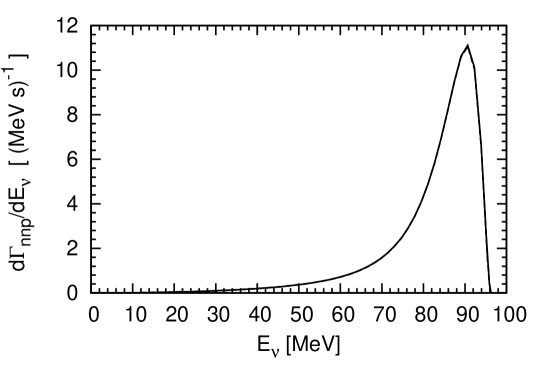
Figure 10: The differential capture rates ${d\Gamma}_{nnp}/{dE_{\nu}}$ for the $\mu^{-}+^{3}{\rm He}\rightarrow\nu_{\mu}+n+n+p$ process calculated with the AV18 potential av18 and using a full solution of Eq. (50) with $V_{4}^{(1)}=0$. The curves representing results of the calculations employing all partial wave states with $j\leq 3$ ($j\leq 4$) in the 2N subsystem are depicted with dashed (solid) curves. The maximal total 3N angular momentum is $J_{max}=\frac{9}{2}$.

For the $\mu^{-}+^{3}{\rm He}\rightarrow\nu_{\mu}+n+n+p$ reaction we show in Fig. 10 that the convergence of the differential capture rate ${d\Gamma}_{nnp}/{dE_{\nu}}$ with respect to the number of partial wave states used in the full calculations is also very good. Comparing the shapes of ${d\Gamma}_{nd}/{dE_{\nu}}$ and ${d\Gamma}_{nnp}/{dE_{\nu}}$ we see that the latter becomes significantly different from zero at smaller neutrino energies. The calculations are based in this case on the AV18 av18 nucleon-nucleon potential and 3N force effects are neglected. In Fig. 11 we show 3N force effects adding the Urbana IX 3N force to the Hamiltonian. The peak reduction caused by the 3N force amounts to about $19\$% which is quite similar to the two-body break-up case. Note that this dependence on the 3N interaction, or essentially on the trinucleon binding energy, is presumably a consequence of the overprediction of the $A=3$ radii when 3N interaction is not included.

We supplement the results presented in Figs. 7–11 by giving the corresponding values of integrated capture rates in Table 3, together with earlier theoretical predictions of Refs. yanox64 ; phili75 ; congl94 and experimental data from Refs. zaimi63b ; auerb65 ; maevx96 ; pra69.012712 . From inspection of the table we can conclude, first of all, that our results are fully at convergence. Secondly, we can estimate 3N force effects for the total rates. For the two break-up reactions separately ($\Gamma_{nd}$ and $\Gamma_{nnp}$) as well as for the total break-up capture rate ($\Gamma_{nd}+\Gamma_{nnp}$) we see a reduction of their values by about $10\$%, when the 3N force is included. Our best numbers (obtained with the AV18 nucleon-nucleon potential and Urbana IX 3N force and the single nucleon current operator) are $\Gamma_{nd}\ =\ 544\ {\rm s}^{-1}$, $\Gamma_{nnp}\ =\ 154\ {\rm s}^{-1}$ and $\Gamma_{nd}+\Gamma_{nnp}\ =\ 698\ {\rm s}^{-1}$ and can be compared with the available experimental data gathered in Table 3, finding an overall nice agreement between theory and experiment for $\Gamma_{nd}+\Gamma_{nnp}$, except for the two results of Refs. phili75 ; congl94 . The experimental uncertainties are however quite large. When comparing with the latest experimental values of Ref. pra69.012712 , we find that our results for $\Gamma_{nnp}$ are smaller than the experimental values and fall within the experimental estimates for $\Gamma_{nd}$ and $\Gamma_{nd}+\Gamma_{nnp}$. We expect that our predictions will be changed by about 10 %, when many body current operators are included in our framework, as in the case of $\mu^{-}+^{3}{\rm He}\rightarrow\nu_{\mu}+^{3}{\rm H}$.

V.1 Analysis of the most recent experimental data for the differential capture rates

Next we embark on an analysis of experimental differential capture rates ${d\Gamma}_{nd}/{dE_{d}}$ and ${d\Gamma}_{nnp}/{dE_{p}}$ published in Ref. pra69.012712 . For a number of deuteron and proton energies these quantities are averaged over 1 MeV-wide energy intervals and presented in the form of tables. The tables contain experimental results normalized to 1 in given energy regions as well as absolute values. The data and their uncertainties have been obtained by two different methods so in each case two data sets are available. The first method uses Monte Carlo simulations and $\chi^{2}$ minimization procedure to compare simulated results, depending on a set of parameters, with experimental events. In the second approach a Bayesian estimation is used to determine the energy distributions of protons and deuterons emitted in the caption reactions.

One could, in principle, prepare a dedicated kinematics to deal with this kind of energy bins, as we did in Ref. romek . Our approach is now, however, quite different and very simple. We have already calculated the capture rates ${d\Gamma}_{nd}/{dE_{\nu}}$ and ${d\Gamma}_{nnp}/{dE_{\nu}}$ on a dense grid (60 points) of neutrino energies, solving for each neutrino energy the corresponding Faddeev-like equation (50). These neutrino energies are distributed uniformly in the whole kinematical region and some extra points are calculated close to the maximal neutrino energy. This dense grid allows us to use the formulas and codes which calculate the total ${\Gamma}_{nd}$ (54) and ${\Gamma}_{nnp}$ (57) capture rates, performing integrals over the whole phase spaces. The sole difference is that in the calculation for a given energy interval only contributions to the corresponding total capture rate with a proper kinematical “signature” are summed.

This kinematical “signature” is easy to obtain. In the case of the two-body break-up reaction it is given by Eq. (55), which can be used to calculate the deuteron momentum and thus its kinetic energy. Two examples showing the distributions of “events” for two deuteron energy intervals in the $E_{\nu}-E_{d}$ plane are given in Fig. 12. The central deuteron energies are 15.5 MeV and 20.5 MeV. In this case the events are generated by different ($E_{\nu}$, $\theta_{q_{0}}$) pairs.

For the three-body break-up reaction the proton energy can be evaluated from Eqs. (58). Again we demonstrate in Fig. 13 two examples showing the distributions of proton “events” for two proton energy intervals in the $E_{\nu}-E_{p}$ plane. (The central proton energies are 25.5 and 35.5 MeV.) We see much more events than in the deuteron case, now generated with 60 uniformly distributed $E_{\nu}$ points, 36 uniformly distributed $\theta_{q}$ values of the relative momentum ${\bf q}$ and 32 values of the magnitude of $q\equiv\mid{\bf q}\mid$. Compared to the deuteron case, the “events” come from much broader neutrino energy range.

We show in Fig. 14 the capture rates $\langle{d\Gamma}_{nd}/{dE_{d}}\rangle$ for the $\mu^{-}+^{3}{\rm He}\rightarrow\nu_{\mu}+n+d$ process averaged over 1 MeV deuteron energy bins, calculated with various 3N dynamics and compared to the two sets of experimental data presented in Table VI of Ref. pra69.012712 . We show the results both on the logarithmic and linear scales. Our simplest plane wave calculations (dash-dotted curves) describe the data well only for small neutrino energies. Predictions based on the full solution of Eq. (50) without (dashed curves) and with (solid curves) a 3N force clearly underestimate the data by nearly a factor of $2$. If the Urbana IX 3N force urbana is added to the 3N Hamiltonian based on the AV18 potential av18 , the agreement with the data is slightly improved. The symmetrized plane wave approximation overshoots the data for smaller neutrino energies and drops much faster than data at higher neutrino energies.

The situation for the averaged capture rates $\langle{d\Gamma}_{nnp}/{dE_{p}}\rangle$ in the case of the $\mu^{-}+^{3}{\rm He}\rightarrow\nu_{\mu}+n+n+p$ reaction is demonstrated in Fig. 15. Here we compare our predictions obtained with the full solution of Eq. (50) without (dashed curve) and with (solid curve) the Urbana IX 3N force urbana to the experimental data evaluated using two methods and shown in Table V of Ref. pra69.012712 . Both types of theoretical results underestimate the data for smaller proton energies and lie much higher than the data for higher proton energies. The inclusion of the 3N force does not bring the theory closer to the data and the 3N force effects are quite tiny.

These two comparisons raise the question whether the calculations of the total rates $\Gamma_{nd}$ and $\Gamma_{nnp}$ (where we at least roughly agree with the data) are consistent with the calculations of the (averaged) differential rates $\langle{d\Gamma}_{nd}/{dE_{d}}\rangle$ and $\langle{d\Gamma}_{nnp}/{dE_{p}}\rangle$ (where we disagree with the data). We have checked that this is the case, calculating $\Gamma_{nd}(E_{\nu}<90\ {\rm MeV})$ in two ways. First we used the information given by ${d\Gamma}_{nd}/{dE_{\nu}}$. In the second calculation we generated corresponding “events” for all deuteron energies provided that $E_{\nu}<90\ {\rm MeV}$ and later used the code for $\langle{d\Gamma}_{nd}/{dE_{d}}\rangle$ to sum the corresponding contributions.

One might also worry if the extrapolation of the experimental results (necessary to arrive at the total rates) made by the authors of Ref. pra69.012712 is justified. From Figs. 5 and 6 it is clear that the data for these two reactions do not cover the region of neutrino energies greater than $90\$ MeV. From our calculations we can see that the total capture rates receive decisive contributions just from this region. In the two-body break-up case this contribution amounts to nearly $70\$%. The simple formula used by the authors of Ref. pra69.012712 to represent the dependence $\langle{d\Gamma}_{nd}/{dE_{d}}\rangle$ on the deuteron energy might not work well for all the deuteron energies. This means that our agreement with experimental data for the total rates from Ref. pra69.012712 could be more or less accidental. At the moment our theoretical framework is not complete and this question should be revisited when the calculations with the more complete current operator are performed.

Finally, we would like to mention that we used these more exclusive observables, $\langle{d\Gamma}_{nd}/{dE_{d}}\rangle$ and $\langle{d\Gamma}_{nnp}/{dE_{p}}\rangle$, to verify the convergence of the full results with respect to the total angular momentum of the final 3N system, $J$. In Fig. 16 we show results of calculations performed with $J\leq\frac{1}{2}$, $J\leq\frac{3}{2}$, $J\leq\frac{5}{2}$, $J\leq\frac{7}{2}$, $J\leq\frac{9}{2}$. corresponding to Figs. 14 and 15. The convergence is extremely rapid, especially in the case of the 3N break-up reaction and actually $J_{max}=\frac{9}{2}$ seems unnecessary large.

Figure 7: The differential capture rates ${d\Gamma}_{nd}/{dE_{\nu}}$ for the $\mu^{-}+^{3}{\rm He}\rightarrow\nu_{\mu}+n+d$ process calculated with the AV18 potential av18 and the single nucleon current operator as a function of the muon neutrino energy, using the symmetrized plane wave (left panel) and a full solution of Eq. (50) with $V_{4}^{(1)}=0$ (right panel). The curves representing results of the calculations employing all partial wave states with $j\leq 3$ ($j\leq 4$) in the 2N subsystem are depicted with dashed (solid) curves. The maximal total 3N angular momentum is $J_{max}=\frac{9}{2}$.

Figure 8: The differential capture rates ${d\Gamma}_{nd}/{dE_{\nu}}$ for the $\mu^{-}+^{3}{\rm He}\rightarrow\nu_{\mu}+n+d$ process calculated with the single nucleon current operator and different types of 3N dynamics: plane wave (dash-dotted curve), symmetrized plane wave (dotted curve), full solution of Eq. (50) without (dashed curve) and with 3N force (solid curve). The calculations are based on the AV18 nucleon-nucleon potential av18 and the Urbana IX 3N force urbana and employ all partial wave states with $j\leq 3$ and $J\leq\frac{9}{2}$.

Figure 9: The double differential capture rates ${d^{2}\Gamma}_{nd}/({dE_{\nu}}d{\Omega}_{q_{0}})$ for the $\mu^{-}+^{3}{\rm He}\rightarrow\nu_{\mu}+n+d$ process calculated with the single nucleon current operator and using the plane wave (dotted curve), symmetrized plane wave (dashed curve) and full solution of Eq. (50) but with $V_{4}^{(1)}=0$ (solid curve) for two values of the neutrino energy. The calculations are based on the AV18 nucleon-nucleon potential av18 and employ all partial wave states with $j\leq 3$ and $J\leq\frac{9}{2}$.

Figure 11: The differential capture rates ${d\Gamma}_{nnp}/{dE_{\nu}}$ for the $\mu^{-}+^{3}{\rm He}\rightarrow\nu_{\mu}+n+n+p$ process calculated with full solutions of Eq. (50) with $V_{4}^{(1)}=0$ (dashed curve) and with $V_{4}^{(1)}\neq 0$ (solid curve). The calculations are based on the AV18 nucleon-nucleon potential av18 and the Urbana IX 3N force urbana and employ all partial wave states with $j\leq 3$ and $J\leq\frac{9}{2}$.

Figure 12: The ”events” for two selected bins corresponding to Fig. 14 with the central deuteron energy $E_{d}$= 15.5 MeV (left panel) and 20.5 MeV (right panel), generated with 60 uniformly distributed $E_{\nu}$ points in the $[0,E_{\nu}^{max,nnp}]$ interval and 72 uniformly distributed $\theta_{q_{0}}$ values of the relative momentum ${\bf q}_{0}$ (in $[0,\pi]$) as explained in the text. For the selected examples the number of ”events” is approximately equal to 130.

Figure 13: The ”events” for two selected bins corresponding to Fig. 15 with the central proton energy $E_{p}$= 25.5 MeV (left panel) and 35.5 MeV (right panel), generated with 60 uniformly distributed $E_{\nu}$ points, 36 uniformly distributed $\theta_{q}$ values of the relative momentum ${\bf q}$ and 32 values of the magnitude of ${\bf q}$ (see text for a detailed explanation). For these two examples the number of ”events” is approximately 1000.

Figure 14: The capture rates $\langle{d\Gamma}_{nd}/{dE_{d}}\rangle$ for the $\mu^{-}+^{3}{\rm He}\rightarrow\nu_{\mu}+n+d$ process averaged over 1 MeV deuteron energy bins are compared with the experimental data given in Table VI of Ref. pra69.012712 . In the left (right) panel the experimental data are evaluated using method I (method II) of Ref. pra69.012712 . The notation for the curves is the same of Fig. 8.

Figure 15: The capture rates $\langle{d\Gamma}_{nnp}/{dE_{p}}\rangle$ for the $\mu^{-}+^{3}{\rm He}\rightarrow\nu_{\mu}+n+n+p$ process averaged over 1 MeV proton energy bins are compared with the experimental data shown in Table V of Ref. pra69.012712 . In the left (right) panel the experimental data are evaluated using method I (method II) of Ref. pra69.012712 . The notation for the curves is the same of Fig. 11.

Figure 16: Convergence of the full results (without a 3N force) with respect to the total angular momentum of the final 3N system corresponding to Figs. 14 (left panel) and 15 (right panel). Curves show results of calculations with $J\leq\frac{1}{2}$ (double dashed), $J\leq\frac{3}{2}$ (dash-dotted), $J\leq\frac{5}{2}$ (dotted), $J\leq\frac{7}{2}$ (dashed) and $J\leq\frac{9}{2}$ (solid).

Table 3: Capture rates for the $\mu^{-}+^{3}{\rm He}\rightarrow\nu_{\mu}+n+d$ ($\Gamma_{nd}$) and $\mu^{-}+^{3}{\rm He}\rightarrow\nu_{\mu}+n+n+p$ ($\Gamma_{nnp}$) processes calculated with the AV18 av18 nucleon-nucleon potential and the Urbana IX urbana 3N force, using the single nucleon current and describing the final states just in plane wave (PW), symmetrized plane wave (SPW), and including final state interaction (full). Early theoretial predictions from Refs. yanox64 ; phili75 ; congl94 are also shown as well as experimental data are from Refs. zaimi63b ; auerb65 ; maevx96 ; pra69.012712 .

	capture rate $\Gamma$ in s-1
	$\Gamma_{nd}$			$\Gamma_{nnp}$	$\Gamma_{nd}+\Gamma_{nnp}$
	PW	SPW	full	full	full
AV18 ($j_{max}=3$)	1917	2046	604	169	773
AV18 ($j_{max}=4$)	1917	2046	606	170	776
AV18+Urbana IX ($j_{max}=3$)	1853	1956	544	154	698
earlier theoretical predictions:
A.F. Yano yanox64	510			160	670
A.C. Philips et al. phili75	414			209	623
J.G. Congleton congl94					650
experimental results:
O.A. Zaĭmidoroga et al. zaimi63b					$660\pm 160$
L.B. Auerbach et al. auerb65					$665\>\>^{+\>170}_{-\>430}$
E.M. Maev et al. maevx96					$720\pm 70$
V.M. Bystritsky et al. pra69.012712 :
method I	$491\pm 125$			$187\pm 11$	$678\pm 126$
method II	$497\pm 57$			$190\pm 7$	$687\pm 60$

V.2 Analysis of the older experimental data for the differential capture rates

In this subsection we provide an analysis of experimental differential capture rates ${d\Gamma}_{nnp}/{dE_{p}}$ and ${d\Gamma}_{nd}/{dE_{d}}$ published in Refs. datainromek1 ; datainromek2 . For each reaction two data sets were obtained with two different detectors.

The data for the ${d\Gamma}_{nnp}/{dE_{p}}$ capture rate are to be found in Table I of Ref. datainromek2 . These data points were averaged over 5-MeV-wide energy bins and our theoretical predictions are prepared consistently. The average procedure has been carried out in the same way as described is Sec. V.1. The fact that in this case the proton energy bins are five times larger poses no additional difficulty. We have noticed that this additional average over wider proton energy bins does not change significantly the representation of our calculations (at least on the logarithmic scale). In Fig. 17 we see that our calculations are in fair agreement with data for $E_{p}\leq 32$ MeV but clearly overshoot the data for the higher proton energies.

The data set for the ${d\Gamma}_{nd}/{dE_{d}}$ capture rate consists of three points only. They are given in Table III and shown in Fig. 9 of Ref. datainromek2 . These data points are compared with our theoretical predictions (based on different types of 3N dynamics) averaged over 1-MeV-wide energy bins. (That means that we use the same results as in the previous subsection.) This bin width corresponds closely to the horizontal errors bars of the three experimental points. In Fig. 18 the simplest plane wave prediction seems to be consistent with the lower energy datum, while the symmetrized plane wave result agrees with the higher energy data. The full results both neglecting and including 3N force effects underestimate also the data from Refs. datainromek1 ; datainromek2 , missing them by 40 % – 60 %. The same data were analyzed by some of the authors of the present paper in Ref. romek with older nucleon-nucleon forces and without 3N potentials. Here we do not confirm the results of Ref. romek , which showed a big difference between the full and symmetrized plane wave predictions. This might indicate some problems in calculations of Ref. romek and will be further investigated.

Figure 17: The capture rates $\langle{d\Gamma}_{nnp}/{dE_{p}}\rangle$ for the $\mu^{-}+^{3}{\rm He}\rightarrow\nu_{\mu}+n+n+p$ process averaged over 5 MeV proton energy bins are compared with the experimental data shown in Table I of Ref. datainromek2 . Circles and triangles are used to represent data taken at two different detectors. The notation for the curves is the same of Fig. 11.

Figure 18: The capture rates $\langle{d\Gamma}_{nd}/{dE_{d}}\rangle$ for the $\mu^{-}+^{3}{\rm He}\rightarrow\nu_{\mu}+n+d$ process averaged over 1 MeV deuteron energy bins are compared with the experimental data given in Table III of Ref. datainromek2 . The notation for the curves is the same of Fig. 8.

VI Summary and conclusions

A consistent framework for the calculations of all muon capture processes on the deuteron, ³He and other light nuclei should be ultimately prepared. This requires that the initial and final nuclear states are calculated with the same Hamiltonian and that the weak current operator is “compatible” with the nuclear forces. If results of such calculations can be compared with precise experimental data, our understanding of muon capture (and other) important weak reactions will be definitely improved.

In the present paper we studied the $\mu^{-}+^{2}{\rm H}\rightarrow\nu_{\mu}+n+n$, $\mu^{-}+^{3}{\rm He}\rightarrow\nu_{\mu}+^{3}{\rm H}$, $\mu^{-}+^{3}{\rm He}\rightarrow\nu_{\mu}+n+d$ and $\mu^{-}+^{3}{\rm He}\rightarrow\nu_{\mu}+n+n+p$ reactions in the framework close to the potential model approach of Ref. prc83.014002 but (except for one attempt) with the single nucleon current operator. Contrary to Ref. prc83.014002 , we work exclusively in the momentum space. In all the cases we check carefully that the nonrelativistic kinematics can be safely used and outline the adopted approximations. We also prove the convergence of our results with respect to the number of partial wave states used in our calculations.

In the case of the $\mu^{-}+^{2}{\rm H}\rightarrow\nu_{\mu}+n+n$ reaction we employed our scheme, which totally avoids standard partial wave decomposition to cross check further elements of our framework. We supplement information given in the literature by showing some predictions for the quadruplet differential and total capture rates. Already in the 2N system we have developed an easy and efficient way to deal with PWD of any single nucleon operator. This scheme is then employed also in the reactions with ³He.

We give first realistic predictions for the differential $d\Gamma_{nd}/dE_{\nu_{\mu}}$ and $d\Gamma_{nnp}/dE_{\nu_{\mu}}$ capture rates as well as for the corresponding total capture rates $\Gamma_{nd}$ and $\Gamma_{nnp}$. Our numbers calculated with the AV18 nucleon-nucleon potential av18 and the 3N Urbana IX potential urbana are 544 s^-1 ($\mu^{-}+^{3}{\rm He}\rightarrow\nu_{\mu}+n+d$) and 154 s^-1 ($\mu^{-}+^{3}{\rm He}\rightarrow\nu_{\mu}+n+n+p$).

Our analysis of the experimental data from Ref. pra69.012712 reveals some contradictions. We agree roughly with the total capture rates but fail to reproduce the differential capture rates. Our results might indicate that the extrapolations and the experimental results on the total capture rates published in Ref. pra69.012712 should be reconsidered. Finally, we are well aware that the full understanding of the muon capture processes requires the inclusion of at least 2N contributions to the nuclear current operators. However, the work presented here is a first step to perform a complete calculation in the near future. Work along this line is currently underway. Nevertheless, the presented predictions will serve as an important benchmark for the future.

References

• (1) D.F. Measday, Phys. Rep. 354, 243 (2001).
• (2) T. Gorringe and H.W. Fearing, Rev. Mod. Phys. 76, 31 (2004).
• (3) P. Kammel and K. Kubodera, Annu. Rev. Nucl. Part. Sci. 60, 327 (2010).
• (4) L.E. Marcucci, M. Piarulli, M. Viviani, L. Girlanda, A. Kievsky, S. Rosati, and R. Schiavilla, Phys. Rev. C 83, 014002 (2011).
• (5) L.E. Marcucci, Int. J. Mod. Phys. A 27 1230006 (2012).
• (6) L.E. Marcucci, R, Schiavilla, S. Rosati, A. Kievsky, and M. Viviani, Phys. Rev. C 66, 054003 (2002).
• (7) L.E. Marcucci, R. Schiavilla, M. Viviani, A. Kievsky, S. Rosati, and J.F. Beacom, Phys. Rev. C 63, 015801 (2000).
• (8) L.E. Marcucci, A. Kievsky, S. Rosati, R. Schiavilla, and M. Viviani, Phys. Rev. Lett. 108, 052502 (2012).
• (9) R. Skibiński, J. Golak, H. Witała, and W. Glöckle, Phys. Rev. C59, 2384 (1999).
• (10) J. Golak, R. Skibiński, H. Witała, W. Glöckle, A. Nogga, and H. Kamada, Phys. Rept. 415, 89 (2005).
• (11) R. Skibiński, J. Golak, H. Witała, W. Glöckle, and A. Nogga, Eur. Phys. J. A 24, 11 (2005).
• (12) A. Kievsky, S. Rosati, M. Viviani, L.E. Marcucci, and L. Girlanda, J. Phys. G 35, 063101 (2008).
• (13) R.B. Wiringa, V.G.J. Stoks, and R. Schiavilla, Phys. Rev. C 51, 38 (1995).
• (14) B.S. Pudliner, V.R. Pandharipande, J. Carlson, Steven C. Pieper, and R.B. Wiringa, Phys. Rev. C 56, 1720 (1997).
• (15) V.M. Bystritsky, V.F. Boreiko, M. Filipowicz, V.V. Gerasimov, O. Huot, P.E. Knowles, F. Mulhauser, V.N. Pavlov, L.A. Schaller, H. Schneuwly, V.G. Sandukovsky, V.A. Stolupin, V.P. Volnykh, and J. Woźniak, Phys. Rev. A 69, 012712 (2004).
• (16) W.J. Cummings, G.E. Dodge, S.S. Hanna, B.H. King, S.E. Kuhn, Y.M. Shin, R. Helmer, R.B. Schubank, N.R. Stevenson, U. Wienands, Y.K. Lee, G.R. Mason, B.E. King, K.S. Chung, J.M. Lee, and D.R. Rosenzweig, Phys. Rev. Lett. 68, 293 (1992).
• (17) S.E. Kuhn, W.J. Cummings, R. Helmer, R.B. Schubank, G.E. Dodge, S.S. Hanna, B.H. King, Y.M. Shin, J.G. Congleton, N.R. Stevenson, U. Wienands, Y.K. Lee, G.R. Mason, B.E. King, K.S. Chung, J.M. Lee, and D.R. Rosenzweig, Phys. Rev. C 50, 1771 (1994).
• (18) J.D. Walecka, Theoretical Nuclear and Subnuclear Physics, Oxford University Press, New York, 1995.
• (19) J.D. Bjorken, S.D. Drell, Relativistic Quantum Mechanics, McGraw-Hill Science/Engineering/Math, 1998.
• (20) D. Bailin, Weak interactions, Adam Hilger, Bristol, 1982.
• (21) G. Shen, L.E. Marcucci, J. Carlson, S. Gandolfi, and R. Schiavilla, Phys. Rev.  C 86 035503 (2012).
• (22) K. Topolnicki, J. Golak, R. Skibiński, A.E. Elmeshneb, W. Glöckle, A. Nogga, and H. Kamada, Few-Body Syst. 54, 2223 (2013).
• (23) R. Machleidt, Adv. Nucl. Phys. 19, 189 (1989).
• (24) E. Epelbaum, W. Glöckle, and U.-G. Meißner, Nucl. Phys. A 747, 362 (2005).
• (25) I.-T. Wang et al., Phys. Rev. 139, B1528 (1965).
• (26) A. Bertin et al., Phys. Rev. D 8, 3774 (1973).
• (27) G. Bardin et al., Nucl. Phys. A 453, 591 (1986).
• (28) M. Cargnelli et al., Workshop on fundamental $\mu$ physics, Los Alamos, 1986, LA 10714C; Nuclear Weak Process and Nuclear Structure, Yamada Conference XXIII, ed. M. Morita, H. Ejiri, H. Ohtsubo, and T. Sato (Word Scientific, Singapore), p. 115 (1989).
• (29) J. Golak, D. Rozp$\scriptstyle\iota$edzik, R. Skibiński, K. Topolnicki, H. Witała, W. Glöckle, A. Nogga, E. Epelbaum, H. Kamada, Ch. Elster, and I. Fachruddin, Eur. Phys. J. A 43, 241 (2010).
• (30) R. Skibiński, J. Golak, K. Topolnicki, H. Witała, H. Kamada, W. Glöckle, and A. Nogga, Eur. Phys. J. A 47, 48 (2011).
• (31) Wolfram Research, Inc., Mathematica${}^{\ooalign{\hfil\raise 0.0pt\hbox{\scriptsize R}\hfil\crcr\text{$\mathchar 525\relax$}}}$, Version 9.0, Champaign, IL (2012).
• (32) D. Rozp$\scriptstyle\iota$edzik, J. Golak, S. Kölling, E. Epelbaum, R. Skibiński, H. Witała, and H. Krebs, Phys. Rev. C 83, 064004 (2011).
• (33) P. Ackerbauer et al., Phys. Lett. B 417, 224 (1998).
• (34) A.F. Yano, Phys. Rev. Lett. 12, 110 (1964).
• (35) A.C. Philips, F. Roig, and J. Ros, Nucl. Phys. A 237, 493 (1975).
• (36) J.G. Congleton, Nucl. Phys. A 570, 511 (1994).
• (37) O.A. Zaĭmidoroga et al., Phys. Lett. 6, 100 (1963).
• (38) L.B. Auerbach et al., Phys. Rev. 138, B127 (1965).
• (39) E.M. Maev et al., Hyp. Interact. 101/102, 423 (1996).