Impurity cyclotron resonance of anomalous Dirac electrons in graphene

Abstract

We have investigated a new feature of impurity cyclotron resonances common to various localized potentials of graphene. A localized potential can interact with a magnetic field in an unexpected way in graphene. It can lead to formation of anomalous boundstates that have a sharp peak with a width $R$ in the probability density inside the potential and a broad peak of size magnetic length $\ell$ outside the potential. We investigate optical matrix elements of anomalous states, and find that they are unusually small and depend sensitively on magnetic field. The effect of many-body interactions on their optical conductivity is investigated using a self-consistent time-dependent Hartree-Fock approach (TDHFA). For a completely filled Landau level we find that an excited electron-hole pair, originating from the optical transition between two anomalous impurity states, is nearly uncorrelated with other electron-hole pairs, although it displays a substantial exchange self-energy effects. This absence of correlation is a consequence of a small vertex correction in comparison to the difference between renormalized transition energies computed within the one electron-hole pair approximation. However, an excited electron-hole pair originating from the optical transition between a normal and an anomalous impurity states can be substantially correlated with other electron-hole states with a significant optical strength.

1 Introduction

A Dirac electron[1, 2, 3] moving in a rotationally invariant, localized, and smoothly varying potential $V(r)$ is described by the Hamiltonian

$$H=v_{F}\vec{\sigma}\cdot(\vec{p}+\frac{e}{c}\vec{A})+V(r),$$ (1)

where $\vec{\sigma}=(\sigma_{x},\sigma_{y})$ and $\sigma_{z}$ are Pauli spin matrices ($\vec{p}$ is two-dimensional momentum). The shape of $V(r)$ can be parabolic, Coulomb, and Gaussian. Half-integer angular momentum $J$ is a good quantum number and wavefunctions of eigenstates have the form

$$\Psi^{J}(r,\theta)=\left(\begin{array}[]{c}\chi_{A}(r)e^{i(J-1/2)\theta}\\ \chi_{B}(r)e^{i(J+1/2)\theta}\end{array}\right).$$ (2)

It consists of A sublattice and B sublattice radial wavefunctions $\chi_{A}(r)$ and $\chi_{B}(r)$ with channel angular momenta $J-1/2$ and $J+1/2$, respectively. The half-integer angular momentum quantum numbers have values $J=\pm 1/2,\pm 3/2,\cdots$. The Hamiltonian has several unusual features not present in the case of massful electrons. A simple scaling analysis[4] suggests that a localized potential $V(r)$ can act as a strong perturbation, and that it can be even more singular in graphene than in ordinary two-dimensional systems of massful electrons: the kinetic term of Dirac Hamiltonian scales as $1/r$ while the potential term scales as $1/r$ and $1/r^{2}$ for Coulomb and Gaussian short-range potentials[5], respectively. The other unusual feature is the presence of quasibound states with complex energies[6, 7].

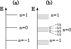
Figure 1: (a) Schematic drawing of degenerate LL energies of graphene. LL energy is $nE_{M}$, where $n=...-1,0,1,...$ is LL index and $E_{M}=\hbar v_{F}/\ell=26(B\textrm{[T]})^{1/2}\textrm{[meV]}$ is the characteristic energy scale of graphene LLs. (b) When an attractive localized potential is present LL energies split into discrete energies. Fractions indicate values of angular momentum $J$.

These effects show up differently in a magnetic field $\vec{B}$ applied perpendicular to the two-dimensional plane (the vector potential $\vec{A}$ is given in a symmetric gauge). In the absence of $V(r)$ eigenenergies form degenerate Landau level (LL) energies while they split into discrete energies when $V(r)$ is present, see Fig.1. They can form true boundstates with real energies[7, 8, 9] in contrast to the case of no magnetic field. Moreover, in addition to the magnetic length, $\ell=25.66(B\textrm{[T]})^{-1/2}\textrm{[nm]}$, a new length scale $R$ is introduced in the wavefunction: boundstates with a s-channel angular momentum component can become anomalous and develop a sharp peak of a width $R$ inside the potential and a broad peak of size magnetic length $\ell$ outside the potential[10]. Although the effect of the potential is strong it is partly mitigated by Klein tunneling, and there is a competition between the two length scales $R$ and $\ell$: the peak is strong in the regime $R/\ell<1$, but small in the regime $R/\ell>1$ (in the limit $R/\ell\rightarrow 0$ it diverges). These states are present in various potentials: regularized Coulomb[11, 12], parabolic[7, 13], and finite-range potentials[8, 10], see Fig.2(a), (b), and (c).

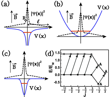
Figure 2: Schematic display of probability density of anomalous states (small peak has width $R$ and broad peak $\ell$). (a) regularized Coulomb potential, (b) parabolic potential, and (c) Gaussian potential. Horizontal lines indicate the energy levels. (d) Energy splitting of $n=0$ (chiral) and $1$ (nonchiral) LLs is shown. Filled squares represent occupied $n=0$ LL states and open circles represent empty $n=1$ LL states. Symbol A stands for an anomalous state. Arrows indicate optical transitions.

However, experimentally it is unclear how to probe these anomalous states. We propose in this paper that they can lead to a new feature in impurity cyclotron resonances between boundstates of LLs[14, 15], shown in Fig.2(d). Optical properties in a magnetic field have several new features not present in a quantum dot in zero magnetic field[16]: the bulk $n=0$ LL states are all chiral (one-component) while the states of other LLs are nonchiral (two-component). As a consequence, the $n=0$ LL has only one anomalous state while the $n=1$ LL has two, see Eq.(2). The optical transitions originating from these states depicted in Fig.2(d). Another unique feature of optical transitions involving anomalous boundstates is that their optical matrix elements are rather small since their wavefunctions are peaked at $r=0$ (this is explicitly shown in Sec.2). Their optical conductivity is thus smaller than those of the usual boundstates. In addition, since the optical strength depends sensitively on magnetic field, we suggest that a magnetic field can serve as an experimental control parameter for detecting the new magnetospectroscopic feature. The electron-electron Coulomb interaction[17] may also affect these transitions. The energy scale of the electron-electron Coulomb interaction is significant in graphene at all values of magnetic fields $B$[18], and each optically excited state is expected to be a correlated many-body state, containing a linear combination of several electron-hole pair states. This effect may change the value of the optical strength. We have investigated this issue for a completely filled LL by computing many-body correlated states within TDHFA[19, 20, 21, 22, 23] and have calculated the optical conductivity. In contrast to the naive expectation, we find that an excited electron-hole pair originating from the optical transition between two anomalous impurity states (see Fig.2) is nearly uncorrelated with other electron-hole states, despite displaying substantial exchange self-energy effects. This absence of correlation is a consequence of a small vertex correction in comparison to the difference between renormalized transition energies computed within the one electron-hole pair approximation. Many-body interactions do not enhance the strength of the optical conductivity of this transition. However, an excited electron-hole pair originating from the optical transition between a normal and an anomalous impurity states (see Fig.2) can be substantially correlated with other electron-hole pairs with a significant optical strength.

This paper is organized as follows. In Sec.2 the optical matrix element of anomalous states is shown to be small using an idealized impurity model. The many-body version of the Kubo formula of optical conductivity is given in Sec.3. How the self-energy correction of a singly occupied LL state affects the optical conductivity is evaluated in Sec.4. In Sec.5 we investigate how important vertex corrections are for a completely filled LL. The final section 6 includes a summary and discussion.

2 Model potential: optical matrix elements of anomalous states

In order to compute the optical conductivity of anomalous states accurately we first solve exactly the single impurity problem, and apply the TDHFA using these solutions. A similar method was used for massful electrons confined in a quantum dot[23]. We study optical properties of anomalous states using a simple model potential. We choose a cylindrical impurity potential[8] since its eigenstates and eigenvalues can be solved exactly in the presence of a magnetic field. This potential captures essential features of anomalous states of parabolic, Coulomb, and Gaussian potentials. The potential has the shape

$$V_{I}(\vec{r})=\left\{\begin{array}[]{c}V_{I}\ \ \ \ r<R\\ 0\ \ \ \ \ r>R\end{array}\right.,$$ (5)

where $V_{I}$ is the strength of the potential and $R$ is the radius of the cylinder. According to Eq.(2) the impurity state $|n,J\rangle$ of $n$th LL with conserved angular momentum quantum number $J$ has the following form of wavefunction $\Psi_{n}^{J}(\vec{r})$

$$\langle\vec{r}|n,J\rangle=\Psi_{n}^{J}(r,\theta)=\left(\begin{array}[]{c}\chi^{l_{A}}_{n,A}(r)e^{i(J-1/2)\theta}\\ \chi^{l_{B}}_{n,B}(r)e^{i(J+1/2)\theta}\end{array}\right),$$ (8)

where the A-component has orbital angular momentum $l_{A}=J-1/2$ and B-component $l_{B}=J+1/2$. The radial wavefunctions are given in [8, 24]

$$\chi^{l_{\sigma}}_{n,\sigma}(r)\sim e^{\frac{-br^{2}}{2}}r^{n_{\sigma}}\left\{\begin{array}[]{c}\alpha_{\sigma}U(q_{\sigma},1+n_{\sigma},br^{2}),\ \ \ r>R\\ \beta_{\sigma}M(q_{\sigma},1+n_{\sigma},br^{2}),\ \ \ r<R\end{array}\right.,$$ (11)

where the sublattice index $\sigma=A,B$ and $U(x,y,z)$ and $M(x,y,z)$ are confluent hypergeometric functions. The impurity eigenenergy is denoted by $\tilde{\epsilon}_{n,J}$, and is plotted as a function of $J$ for LL indices $n=0$ and $1$ in Fig.2(d).

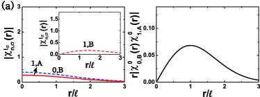
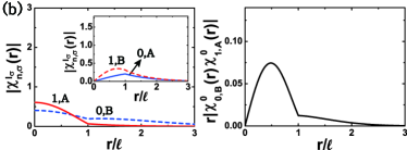
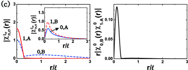
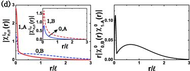
Figure 3: Wavefunction properties of impurity states $|0,-1/2\rangle$ and $|1,1/2\rangle$. Left column: s-wave radial functions $|\chi_{0,B}^{0}(r)|$ (dashed line) and $|\chi_{1,A}^{0}(r)|$ (solid line). Inset: p-wave radial functions $|\chi_{0,A}^{-1}(r)|$ (solid line) and $|\chi_{1,B}^{1}(r)|$ (dashed line). From (a) to (d) the values of parameters are $(\frac{V_{I}}{E_{M}},\frac{R}{\ell})=(0,0),(-2,1),(-7.9,0.3),(-20,0.1)$. Right column: integrand $r\chi_{0,B}^{0}(r)\chi_{1,A}^{0}(r)$ is displayed.

Let us investigate which impurity states $\Psi_{n}^{J}(\vec{r})$ can be anomalous, i.e., which of these states can have s-wave radial functions. It is possible only for states with $J=\pm 1/2$, see Eq.(2). Using confluent hypergeometric functions and Eq.(8) it can be shown that, for $n=0$ LL, only the state $\Psi_{0}^{-1/2}(\vec{r})$ has value at the origin $\Psi_{0}^{-1/2}(0)\neq 0$ since its the B-component radial wavefunction $\chi^{0}_{0,B}(r)$ is s-wave. While, for $n=1$ LL, both $\Psi_{1}^{-1/2}(\vec{r})$ and $\Psi_{1}^{1/2}(\vec{r})$ can be anomalous since their B- and A-components of radial wavefunctions are s-wave, respectively. These states are labeled by $A$ in Fig.2(d). They actually become anomalous when the condition $R/\ell<1$ is satisfied, see Fig.3.

Photons are assumed to be polarized along x-axis, and the optical matrix elements can be computed using the current operator $\vec{j}=v_{F}\vec{\sigma}$[2]. They satisfy the selection rules with the change of LL index $\Delta n=1$ and change of angular momentum $\Delta J=1$[25], and the relevant single-particle optical transitions are of the type $|0,J\rangle\rightarrow|1,J+1\rangle$. The optical matrix element between the relevant anomalous states can be expressed in terms of the corresponding radial wavefunctions (see Eq.(8))

$$\langle 1,1/2|\sigma_{x}|0,-1/2\rangle = \langle e^{i\theta}\chi^{1}_{1,B}|e^{-i\theta}\chi^{-1}_{0,A}\rangle+\langle\chi^{0}_{1,A}|\chi^{0}_{0,B}\rangle$$ (13)

$$= \langle\chi^{0}_{1,A}|\chi^{0}_{0,B}\rangle.$$

In order to understand why this optical matrix element can be small the radial wavefunctions $\chi^{0}_{1,A}(r)$ and $\chi^{0}_{0,B}(r)$ in $\langle\chi^{0}_{1,A}|\chi^{0}_{0,B}\rangle$ are plotted, together with the integrand of $\int drr\chi^{0}_{1,A}(r)^{*}\chi^{0}_{0,B}(r)$, in Fig.3. We see from the shape integrand, Figs.3(b), (c), and (d), that the resulting integral is smaller than the corresponding integral in the absence of the localized potential plotted in Fig.3(a). The actual values of transition matrix elements $|\langle 1,J|\sigma_{x}|0,J^{\prime}\rangle|^{2}$ are given in Table 1 for varies values of $\Big{(}\frac{V_{I}}{E_{M}},\frac{R}{\ell}\Big{)}$. The dependence of the transition matrix elements on the parameters $\Big{(}\frac{V_{I}}{E_{M}},\frac{R}{\ell}\Big{)}$ is non-trivial. Note that they depend significantly on the ratio $R/\ell$, i.e., on magnetic field.

Table 1: Transition matrix elements $|\langle 1,J|\sigma_{x}|0,J^{\prime}\rangle|^{2}$

	$(\frac{1}{2},-\frac{1}{2})$	$(-\frac{1}{2},-\frac{3}{2})$	$(-\frac{3}{2},-\frac{5}{2})$	$(-\frac{5}{2},-\frac{7}{2})$	$(-\frac{7}{2},-\frac{9}{2})$
$(-2,1)$	0.137	0.263	0.377	0.487	0.5
$(-7.9,0.3)$	0.025	0.146	0.5	0.5	0.5
$(-20,0.1)$	0.157	0.341	0.5	0.5	0.5

3 Optical conductivity

We compute the many-body optical conductivity in the presence of a single impurity (when more impurities are present in the dilute limit the total optical conductivity is given by the sum of the optical conductivity of each impurity[26]). We consider excitations from a singly occupied LL or completely filled LL (partially filled LLs cannot be described adequately in TDHFA since screening becomes important). The groundstate is denoted by $|\psi_{F}\rangle$, and it represents either a singly occupied LL or completely filled LL. In this case the optical conductivity consists of a series of discrete peaks.

Generally a many-body excited state can be written as a linear combination of single-electron excited states

$$|\Psi\rangle=\sum_{J}C_{J}|\psi_{J}\rangle,$$ (14)

where single-electron excited states with $\Delta J=1$ are

$$|\psi_{J}\rangle=a^{{\dagger}}_{n^{\prime},J+1}a_{n,J}|\psi_{F}\rangle.$$ (15)

Here the operator $a^{{\dagger}}_{n,J}$ creates an electron in the localized state of $n$th LL with angular momentum $J$. The optical conductivity consists of a series of discrete peaks at the renormalized excitation energies $E_{ex}$

$$\sigma(E)=\sum_{E_{ex}}s(E)\delta(E-E_{ex}),$$ (16)

where $s(E)$ is the optical strength. When this strength is divided by a constant $c=1/(\sqrt{2}E_{M})$ it has dimension of conductivity (if other value of $c$ is chosen the magnitude of this scaled conductivity will be different). The scaled optical strength is computed using the Kubo formula

$$\tilde{s}(E_{ex})=\frac{s(E_{ex})}{1/(\sqrt{2}E_{M})}=\frac{\pi}{2}\frac{e^{2}}{h}\frac{|\langle\Psi|T|\psi_{F}\rangle|^{2}}{\tilde{E}_{ex}},$$ (17)

where the scaled excitation energy is $\tilde{E}_{ex}=E_{ex}/(\sqrt{2}E_{M})$. When photons are polarized along x-axis the optical matrix element is given by $\langle\Psi|T|\psi_{F}\rangle$, where

$$T=\sum_{J}\langle n^{\prime},J+1|\sigma_{x}|n,J\rangle a^{{\dagger}}_{n^{\prime},J+1}a_{n,J}+h.c.$$ (18)

The computed the optical matrix element for $n=0$ and $n^{\prime}=1$ LLs can be written in terms of expansion coefficients $C_{J}$ and the optical many-body matrix elements

$$\langle\Psi|T|\psi_{F}\rangle = C_{-1/2}^{*}\langle 1,1/2|\sigma_{x}|0,-1/2\rangle$$ (19)

$$+ C_{-3/2}^{*}\langle 1,-1/2|\sigma_{x}|0,-3/2\rangle$$

$$+ C_{-5/2}^{*}\langle 1,-3/2|\sigma_{x}|0,-5/2\rangle$$

$$+ C_{-7/2}^{*}\langle 1,-5/2|\sigma_{x}|0,-7/2\rangle$$

$$+ \cdots.$$

4 Singly occupied Landau level

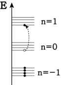
Figure 4: A single electron is in the $n=0$ LL. The LLs $n=-1,-2,...$ are all filled.

Before we investigate the effect of many-body correlations on the optical conductivity of anomalous states we compute it without them and include only self energy effects. This calculation is a good approximation and is experimentally relevant when the $n=0$ LL is occupied by only one electron. In this case only one term survives in the linear combination given by Eq.(14): there is only one excited state with $\Delta n=1$ and $\Delta J=1$, namely $|\psi_{J}\rangle=a^{{\dagger}}_{1,J+1}a_{0,J}|\psi_{F}\rangle$. This implies that many-body correlation effects are not present. However, self-energy corrections are present. The LLs with energies lower than the split $n=0$ energies, i.e., the $n=-1,-2,...$ LLs are all occupied, see Fig.4. Bare impurity eigenenergies $\tilde{\epsilon}_{n,J}$, shown in Fig.2(d), will acquire self-energy corrections originating from interactions with the filled electrons. The renormalized impurity energy is

$$E_{n,J}=\tilde{\epsilon}_{n,J}+\Sigma_{n,J}^{H}+\Sigma_{n,J}^{X}.$$ (20)

The Hartree self-energy originates from the electronic density and ionic potential, and has two parts

$$\Sigma_{m,J}^{H} = \sum_{n^{\prime},J^{\prime}}f_{n^{\prime},J^{\prime}}\langle m,J;n^{\prime},J^{\prime}|V|m,J;n^{\prime},J^{\prime}\rangle$$ (21)

$$- \sum_{n^{\prime},l^{\prime}}f_{n^{\prime},l^{\prime}}\langle m,J;n^{\prime},l^{\prime}|V|m,J;n^{\prime},l^{\prime}\rangle,$$

where electron-electron interaction is $V(r_{1}-r_{2})=\frac{e^{2}}{\epsilon|r_{1}-r_{2}|}$ and the occupation functions $f_{n,J}=1/0$ if $|n,J\rangle$ state is occupied/unoccupied. The second term represents a correction due to uniform ionic potential ($|n,l\rangle$ represents a LL state of graphene in the absence of an impurity potential). The Hartree self-energy corrections are negligibly small. The exchange self-energy is given by

$$\Sigma_{m,J}^{X} = -\sum_{n^{\prime},J^{\prime}}f_{n^{\prime},J^{\prime}}\langle m,J;n^{\prime},J^{\prime}|V|n^{\prime},J^{\prime};m,J\rangle$$ (22)

when $\mathbf{K}$ and $\mathbf{K^{\prime}}$ valleys are uncoupled[27]. Energies corrected by these exchange self-energy corrections are shown in Fig.5.

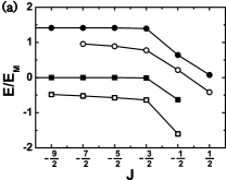
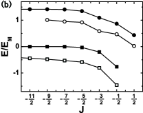
Figure 5: Bare impurity energies $\tilde{\epsilon}_{n,J}$ for $n=0$ and $1$ LL states (filled symbols). Energies corrected by self-energy correction $E_{n,J}$ (open symbols). (a) $V_{I}=-7.9E_{M}$ and $R=0.3\ell$. (b) $V_{I}=-2E_{M}$ and $R=\ell$.

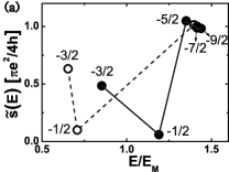
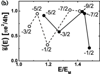
Figure 6: Scaled optical strength as a function of $E$ for transitions between chiral and nonchiral states ($n=0\rightarrow 1$). Open circles represent optical strengths of single particle transitions without many-body effects; the corresponding transitions are indicated as arrows in Fig.2(d). Optical strengths renormalized by self-energy corrections are displayed by filled circles. Each circle is labeled by a fraction, which denotes the initial states $J$ of the optical transitions $(0,J)\rightarrow(1,J+1)$. (a) $V_{I}=-7.9E_{M}$ and $R=0.3\ell$. (b) $V_{I}=-2E_{M}$ and $R=\ell$.

The scaled optical strength of Eq.(17) is given by

$$\tilde{s}(E_{ex})=\frac{\pi}{2}\frac{e^{2}}{h}\frac{|\langle 1,J+1|\sigma_{x}|0,J\rangle|^{2}}{\tilde{E}_{ex}},$$ (23)

where the scaled excitation energy is given by the difference between renormalized impurity energies $\tilde{E}_{ex}=(E_{1,J+1}-E_{0,J})/(\sqrt{2}E_{M})$. The computed scaled optical strengths are shown in Fig.6. Let us first discuss the results in the absence of self-energy corrections. When $(V_{I}/E_{M},R/\ell)=(-2,1)$ the bare transition between anomalous states, $n=0\rightarrow 1$ with $J=-1/2\rightarrow 1/2$, has small optical matrix element $|\langle 0,-1/2|\sigma_{x}|1,1/2\rangle|^{2}=0.137$. The resulting value of the scaled optical strength is also small with the value $0.325\frac{\pi e^{2}}{4h}$, see Fig.6(b). For other bare transitions the optical matrix elements are larger and their scaled optical strengths are bigger $\frac{1}{2}\frac{\pi e^{2}}{4h}<\tilde{s}(E_{ex})<\frac{\pi e^{2}}{4h}$. Similar result also holds for $(V_{I}/E_{M},R/\ell)=(-7.9,0.3)$, see Fig.6(a). We see that the values of the scaled optical strength are almost unchanged by the exchange-self energy corrections (In Fig.6 any two transitions labeled by same $J$ have similar values of strengths). However, the corresponding renormalized excitation energies display significant changes from those of bare transitions.

5 A filled Landau level

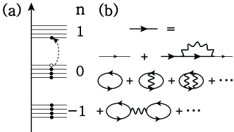
Figure 7: (a) Optical transition from a localized state of the filled $n=0$ LL to a localized state of the empty $n=1$ LL. (b) The self-energy is evaluated in a self-consistent HFA. Renormalized excitation energy is computed within a time-dependent self-consistent HFA including excitonic and depolarization effects.

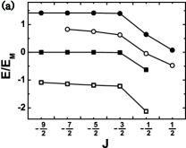
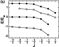
Figure 8: Bare impurity energies $\tilde{\epsilon}_{n,J}$ of $n=0$ (chiral) and $1$ (nonchiral) LLs by the impurity (filled symbols). When the $n=0$ LL is completely filled these energies must be corrected by including self-energies $E_{n,J}$ (open symbols). (a) $V_{I}=-7.9E_{M}$ and $R=0.3\ell$. (b) $V_{I}=-2E_{M}$ and $R=\ell$.

When a LL is completely filled both many-body correlations and self energy effects may be important. Here we investigate how they may affect the optical conductivity of anomalous states. Here we assume that $n=0,-1,-2,...$ LLs are filled. An optical transition leaves a hole in the filled $n=0$ LL, see Fig.7(a). Since there can be several electron-hole excitations with $\Delta J=1$ an eigenstate is given by a linear combination of these electron-hole states. This implies that many-body correlation effects may be important. In this section we evaluate the magnitude of the excitonic and depolarization many-body effects (they are depicted in Fig.7(b)). Since $n=0$ LL is also filled in addition to the $-1,-2,.....$ LLs the exchange self-energy acquires an additional correction in comparison to the case of singly occupied $n=0$ LL. The new exchange self-energies are shown in Fig.8. In this section we explore whether these features can affect the optical conductivity in a significant way.

5.1 Many-body Hamiltonian matrix

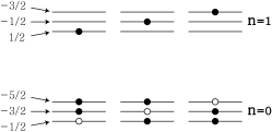
Figure 9: Examples of electron configurations that serve as basis states of the Hamiltonian matrix. First, second, and third states are labeled by $J=-1/2$, $-3/2$, and $-5/2$, respectively (see Eq.(15)).

The electron-hole excitations form basis states of the Hamiltonian matrix. Some of these configuration states are displayed in Fig.9. These electron configurations are coupled to each other by many-body interactions. In a TDHFA[19, 20, 21] the Hamiltonian matrix elements can be split into two parts

$$H_{J,J^{\prime}}=E_{J}^{d}\delta_{J,J^{\prime}}+\Gamma_{J,J^{\prime}}.$$ (24)

The diagonal Hamiltonian matrix elements are

$$E_{J}^{d}=E_{1,J+1}-E_{0,J}+\Gamma_{J,J},$$ (25)

where the interaction energy of the groundstate $E_{G}$ is set to zero. Note that it contains the contribution from the diagonal vertex corrections and that the renormalized single-particle energy $E_{n,J}$ contain self-energy corrections (now $n=0$ LL is also filled, unlike the case studied in Sec.3). The off-diagonal Hamiltonian elements are the vertex corrections and are given by

$$\Gamma_{J,J^{\prime}} = -\langle 0,J;1,J+1|V|0,J^{\prime};1,J^{\prime}+1\rangle$$ (26)

$$+\langle 0,J;1,J+1|V|1,J^{\prime}+1;0,J^{\prime}\rangle,$$

where the first term is the excitonic contribution

$$-E_{ex}=-\langle 0,J;1,J+1|V|0,J^{\prime};1,J^{\prime}+1\rangle$$ (27)

and the second term is the depolarization contribution

$$E_{depol}=\langle 0,J;1,J+1|V|1,J^{\prime}+1;0,J^{\prime}\rangle.$$ (28)

5.2 Excitation energies

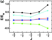
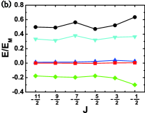
Figure 10: The following quantities in the diagonal elements of the Hamiltonian matrix, see Eq.(29), are plotted as a function of $J$: $\Sigma_{1,J}^{X}-\Sigma_{0,J}^{X}$ (circle), $\Sigma_{1,J}^{H}-\Sigma_{0,J}^{H}$ (square),$-E_{ex}$ (diamond), depolarization (triangle), and renormalization of the bare excitation energy $\Sigma_{1,J}^{X}-\Sigma_{0,J}^{X}+\Gamma_{J,J}$, ignoring the small Hartree corrections (inverted triangle). (a) $V_{I}=-7.9E_{M}$ and $R=0.3\ell$. (b) $V_{I}=-2E_{M}$ and $R=\ell$.

Despite the presence of mixing between different electron configurations, we find that the renormalized transition energy of $|0,J\rangle\rightarrow|1,J+1\rangle$ can be computed approximately using a diagonal approximation: it is equal to $E_{J}^{d}$, see Eq.(25), to compute the values of optical strength accurately one may have to beyond the diagonal approximation. It can be broken into various components

$$H_{J,J}=E_{J}^{d} = (\tilde{\epsilon}_{1,J+1}-\tilde{\epsilon}_{0,J})$$ (29)

$$+ (\Sigma_{1,J+1}^{H}-\Sigma_{0,J}^{H})$$

$$+ (\Sigma_{1,J+1}^{X}-\Sigma_{0,J}^{X})$$

$$+ (-E_{ex}+E_{depol}).$$

Values of these corrections are plotted as a function of $J$ in Fig.10. The exchange self-energy correction $\Sigma_{1,J}^{X}-\Sigma_{0,J}^{X}$ is the most dominant term (circles in Fig.10). This diagonal approximation is physically equivalent to keeping only one electron-hole pair in the calculation.

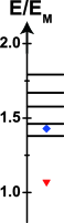
Figure 11: Five eigenenergies obtained by diagonalizing $5\times 5$ Hamiltonian matrix. Lowest bare impurity transition energy $\tilde{\epsilon}_{1,1/2}-\tilde{\epsilon}_{0,-1/2}$ (inverted triangle). Lowest transition energy in the diagonal approximation (diamond) Parameters are $V_{I}=-2E_{M}$ and $R=\ell$.

Corrections to the transition energies beyond the diagonal approximation can be investigated by solving the Hamiltonian matrix, see Eq.(24) (this method is equivalent to including the interaction between different electron-hole pairs). Fig.11 displays obtained transition energies using $5\times 5$ Hamiltonian matrix for $V_{I}=-2E_{M}$. The transition $(n,J)=(0,-3/2)\rightarrow(1,-1/2)$ as the lowest renormalized transition energy $1.38E_{M}$ while the corresponding bare transition energy is $1.071E_{M}$. The deviation between the two values is $22.4\%$. Note that the many-body effects increase the transition energy from the bare value. For this transition the corresponding many-body state has the expansion coefficients $C_{J}=(-0.272,-0.733,-0.594,-0.161,-0.097)$, given by the linear combination Eq.(14). There is a substantial mixing between different electron-pair configurations. Note that $C_{J}$ for $J=-3/2$ and $-5/2$ are dominant. In the diagonal approximation the transition energy is $1.46E_{M}$, which is close to the renormalized value. So despite strong mixing the diagonal approximation given a good estimate of transition energies.

5.3 Results of optical conductivity

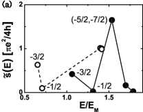
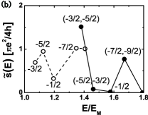
Figure 12: Scaled optical strength as a function of $E$ for transitions between chiral and nonchiral states ($n=0\rightarrow 1$). Open circles represent optical strengths of single particle transitions without many-body effects; the corresponding transitions are indicated as arrows in Fig.2(d). In this figure a set of numbers $(-3/2,-5/2)$ means that the many-body excited state is dominantly a mixture electron-hole pair states $|\psi_{-3/2}\rangle$ and $|\psi_{-5/2}\rangle$ (electron-hole pair states $|\psi_{J}\rangle$ are defined in Eq.(15)). On the other hand, a transition labeled by a single value of $J$ means that the electron-hole pair state $|\psi_{J}\rangle$ is the most dominant one in the linear combination given by Eq.(14). Optical strengths renormalized by self-energy and vertex corrections are displayed by filled circles. (a) $V_{I}=-7.9E_{M}$ and $R=0.3\ell$. (b) $V_{I}=-2E_{M}$ and $R=\ell$.

Let us show the result of the optical conductivity obtained by including full many-body effects. We diagonalize $5\times 5$ Hamiltonian matrices (here we are mostly interested in lower energy excitations than that of magnetoplasmons; a significantly larger Hamiltonian matrix is needed to describe magnetoplasmon physics). The many-body eigenstates are given by the linear combination of electron-hole pair states $|\psi_{J}\rangle$ (see Eq.(14)). The obtained result for the scaled optical strength, given by Eq.(17), is displayed in Fig.12 together with the bare values in the absence of many-body effects.

A transition between two anomalous impurity states is labeled by $-1/2$, see Figs.12 (a) and (b). It is created by the transition between two impurity anomalous states $|0,-1/2\rangle$ and $|1,1/2\rangle$, see Fig.2. Our numerical work shows that it involves dominantly only one electron-hole pair state $|\psi_{-1/2}\rangle$, and is nearly uncorrelated, displaying a small mixing with other electron-hole pair states. We investigate the physical origin of this effect by treating the off-diagonal matrix elements of the many-body Hamiltonian, Eq.(26), as a perturbation and computing the first-order correction to the many-body state. The degree of mixing between the electron-hole pair states $|\psi_{-1/2}\rangle$ and $|\psi_{-3/2}\rangle$ is small since the magnitude of vertex correction between them $\Gamma_{-1/2,-3/2}$ is smaller than the difference between their renormalized transition energies $|E_{-3/2}^{d}-E_{-1/2}^{d}|$ ($E_{J}^{d}$ is computed within the one electron-hole pair approximation and is given in Eq.(25)). Although the optical conductivity of this transition is small, it can be enhanced by tuning the value of magnetic field (see Table 1).

The other transitions between a normal and an anomalous state are labeled by $-3/2$ and $(-3/2,-5/2)$, see Figs.12 (a) and (b). These transitions are created by the optical transition between impurity states $|0,-3/2\rangle\rightarrow|1,-1/2\rangle$ (note that only $|1,-1/2\rangle$ is an anomalous state, see Fig.2). It is nearly uncorrelated for the parameter values $(V_{I},R/\ell)=(-7.9,0.3)$ (see Fig.12(a)). However, this same state is more correlated for $(V_{I},R/\ell)=(-2,1)$, resulting in the state $(-3/2,-5/2)$, see Fig.12(b). This correlated state has a significantly enhanced value of the optical strength in contrast to the state $-3/2$. The interplay between the vertex corrections and the renormalized transition energies can thus affect substantially the optical transitions involving one anomalous state.

6 Summary and discussion

We have investigated a new feature in the impurity cyclotron resonance that is common to various localized potentials of graphene. Application of a magnetic field makes $n=0$ and $n=1$ LL states chiral and nonchiral, respectively. This has a non-trivial implication, leading to only one anomalous state for the $n=0$ LL while two for the $n=1$ LL, see Fig.2. It is a unique feature of physics of finite magnetic fields. The anomalous boundstates are strongly localized inside the well with a broad peak outside the well with width comparable to the magnetic length. In this paper we have proposed that anomalous boundstates may exhibit an unusually small value of magneto-optical conductivity since optical matrix elements of anomalous states are negligible compared to those of ordinary states. The effect of many-body interactions on their optical conductivity is investigated for a completely filled LL using a self-consistent TDHFA. We find that an excited electron-hole state originating from the optical transition between two anomalous impurity states exhibits small correlations with other electron-hole states, despite it displaying substantial exchange self-energy effects. This is a consequence of a small vertex correction in comparison to the difference between renormalized transition energies computed within the one electron-hole pair approximation. We find that many-body interactions do not enhance the strength of its optical conductivity. However, by tuning the value of magnetic field its strength may be enhanced significantly. There is also a transition between a normal and an anomalous impurity states. Unlike the optical transition between two anomalous state, we find, in this case, that the optically created electron-hole pair can be substantially correlated with other electron-hole pairs, and that its optical strength can be significant.

Note that the eigenenergies of a parabolic potential are complex, implying that the lifetime in the potential is finite. For optical studies states with small imaginary part of the eigenenergies are desirable. If the confining potentials vary fast there may be some valley mixing, which leads to splitting of eigenenergies[28]. A tight-binding calculation can be used to investigate this effect.

Recently several infrared absorption experiments of graphene have been performed[29, 30, 31]. We suggest that this type of experiment be performed in magnetic fields on donor impurities or on quantum dot arrays in graphene, just like the case of two-dimensional massful electrons[14, 15, 32]. It would be interesting to observe anomalous transitions in the impurity cyclotron resonance in the regime $R/\ell<1$, and confirm the sensitive dependence of their optical strength on magnetic field. In this paper we considered donor impurities. For acceptors or antidots[28] we can use the transformation $V(r)\rightarrow-V(r)$ with the eigenenergies $E\rightarrow-E$ (eigenstates are unchanged).

References

References

- [1] A. K. Geim and A. H. MacDonald, Phys. Today 60, 35 (2007).
- [2] C. W. J. Beenakker, Rev. Mod. Phys. 80, 1337 (2008).
- [3] A. H. Castro Neto, F. Guinea, N. M. R. Peres, K. S. Novoselov, and A. K. Geim, Rev. Mod. Phys. 81, 109 (2009).
- [4] R. Jackiw, ’Delta function potentials in two- and three-dimensional quantum mechanics’, in M.A.B. Bég Memorial Volume, eds. A. Ali and P. Hoodbhoy (World Scientific, Singapore, 1991).
- [5] For massful electrons kinetic term scales as . The potential is comparable to or weaker than the kinetic term.
- [6] A. Matulis and F. M. Peeters, Phys. Rev. B 77, 115423 (2008); P. G. Silvestrov and K. B. Efetov, Phys. Rev. Lett. 98, 016802(2007).
- [7] G. Giavaras, P. A. Maksym, and M. Roy, J. Phys.: Condens. Matter 21, 102201 (2009).
- [8] P. Recher, J. Nilsson, G. Burkard, and B. Trauzettel, Phys. Rev. B 79, 085407 (2009).
- [9] S. Schnez, K. Ensslin, M. Sigrist, and T. Ihn, Phys. Rev. B 78, 195427 (2008).
- [10] P. S. Park, S. C. Kim, and S. -R. Eric Yang, Phys. Rev. B 84, 085405 (2011).
- [11] S. C. Kim and S. -R. Eric Yang, Annals of Physics 347, 21 (2014). In the case of the impurity Coulomb potential a regularization parameter must be introduced: for and for ( is the dielectric constant). When the strength of the potential is strong this is needed to prevent the spurious effect of Coulomb fall to the center of the potential.
- [12] C. L. Ho and V. R. Khalilov, Phys. Rev. A 61, 032104 (2000); Y. Zhang, Y. Barlas, and K. Yang, Phys. Rev. B 85, 165423 (2012).
- [13] The natural length scale of a parabolic potential is . S. C. Kim, J. W. Lee, and S. -R. Eric Yang, J. Phys.: Condens. Matter 24, 495302 (2012); P. S. Park, S. C. Kim, and S. -R. Eric Yang, Phys. Rev. Lett. 108, 169701 (2012).
- [14] N. C. Jarosik, B. D. McCombe, B. V. Shanabrook, J. Comas, J. Ralston, and G. Wicks, Phys. Rev. Lett. 54, 1283 (1985).
- [15] V. J. Goldman, H. D. Drew, M. Shayegan, and D. A. Nelson, Phys. Rev. Lett. 56, 968 (1986).
- [16] T. Yamamoto, T. Noguchi, and K. Watanabe, Phys. Rev. B 74, 121409(R) (2006); M. Zarenia, A. Chaves, G. A. Farias, and F. M. Peeters, Phys. Rev. B 84, 245403 (2011).
- [17] Optical properties of bulk graphene at have been investigated using various many-body techniques: D. Prezzi, D. Varsano, A. Ruini, A. Marini, and E. Molinari, Phys. Rev. B 77, 041404(R) (2008); L. Yang, J. Deslippe, C. -H. Park, M. L. Cohen, and S. G. Louie, Phys. Rev. Lett. 103, 186802 (2009); W. Wei and T. Jacob, Phys. Rev. B 87, 115431 (2013).
- [18] The dimensionless strength of the electron-electron Coulomb interaction is given by the ratio between the energy scales for the Coulomb interaction and LL energy separation , and note that this dimensionless coupling constant is independent of magnetic field. Hereafter we will set .
- [19] Y. A. Bychkov, S. V. Iordanskii, and G. M. Éliashberg, Pis’ma Zh. Ekps. Teor. Fiz. 33, 152 (1981) [JETP Lett. 33, 143 (1981)].
- [20] C. Kallin and B. I. Halperin, Phys. Rev. B 30, 5655 (1984).
- [21] A. H. MacDonald, J. Phys. C 18, 1003 (1985).
- [22] Y. A. Bychkov and G. Martinez, Phys. Rev. B 77 125417 (2008); R. Roldán, J. -N. Fuchs, and M. O. Goerbig, Phys. Rev. B 82 205418 (2010).
- [23] D. Pfannkuche, V. Gudmundsson, and P. A. Maksym, Phys. Rev. B 47, 2244 (1993). In this paper, just like in our approach, the states of a quantum-dot in a magnetic field are obtained exactly before applying Hartree-Fock method.
- [24] D. Yoshioka, The Quantum Hall Effect (Springer, Berlin, 1998). In the absence of a potential these functions are related to Laguerre polynomials.
- [25] In the presence of a strong impurity potential the selection rule must be relaxed since different LLs get mixed. However, the corresponding transitions have small matrix elements and will be ignored in the following.
- [26] S. -R. Eric Yang and A. H. MacDonald, Phys. Rev. B 42, 10811 (1990).
- [27] J. W. Lee, S. C. Kim, and S. -R. Eric Yang, Solid State Commun., 152, 1929 (2012). In this paper exchange self-energy is computed when and valleys are coupled.
- [28] P. S. Park, S. C. Kim, and S. -R. Eric Yang, J. Phys.: Condens. Matter 22, 375302 (2010).
- [29] V. P. Gusynin, S. G. Sharapov, and J. P. Carbotte, Phys. Rev. Lett. 96, 256802 (2006); ibid. 98, 157402 (2007); J. Phys.: Condens. Matter 19, 026222 (2007).
- [30] L. A. Falkovsky and A. A. Varlamov, Eur. Phys. J. B 56, 281 (2007); L. A. Falkovsky and S. S. Pershoguba, Phys. Rev. B 76, 153410 (2007).
- [31] Z. Q. Li, E. A. Henriksen, Z. Jiang, Z. Hao, M. C. Martin, P. Kim, H. L. Stormer, and D. N. Basov, Nature Phys. 4, 532 (2008); K. F. Mak, M. Y. Sfeir, Y. Wu, C. H. Lui, J. A. Misewich, and T. F. Heinz, Phys. Rev. Lett. 101, 196405 (2008).
- [32] D. Heitmann and J. P. Kotthaus, Phys. Today 46, 56 (1993).