Internal bores and gravity currents in a two-fluid system

Abstract

In this paper, a unified theory of internal bores and gravity currents is presented within the framework of the one-dimensional two-layer shallow-water equations.

The equations represent four basic physical laws: the theory is developed on the basis of these laws. Though the first three of the four basic laws are apparent, the forth basic law has been uncertain. This paper shows first that this forth basic law can be deduced from the law which is called in this paper the conservation law of circulation.

It is then demonstrated that, within the framework of the equations, an internal bore is represented by a shock satisfying the shock conditions that follow from the four basic laws. A gravity current can also be treated within the framework of the equations if the front conditions, i.e. the boundary conditions to be imposed at the front of the current, are known. Basically, the front conditions for a gravity current also follow from the four basic laws. When the gravity current is advancing along a no-slip boundary, however, it is necessary to take into account the influence of the thin boundary layer formed on the boundary; this paper describes how this influence can be evaluated.

It is verified that the theory can satisfactorily explain the behaviour of internal bores advancing into two stationary layers of fluid. The theory also provides a formula for the rate of advance of a gravity current along a no-slip lower boundary; this formula proves to be consistent with some empirical formulae. In addition, some well-known theoretical formulae on gravity currents turn out to be obtainable on the basis of the theory.

1 Introduction

The one-dimensional two-layer shallow-water equations are often used to describe the motion of two superposed fluids of different density in a channel; since the equations are mathematically tractable, the use of them is quite advantageous. Within the framework of these equations, an internal bore is represented by a ‘shock’, i.e. a discontinuity that divides two continuous solutions. The representation enables us to deal with an internal bore without detailed information on its structure. On the other hand, certain boundary conditions are necessary at the position of such a discontinuity to connect the solutions on the two sides of the discontinuity. Our first aim in the present study is to formulate these boundary conditions, i.e. the ‘shock conditions’, appropriate to the equations.

The one-dimensional two-layer shallow-water equations form a system of four partial differential equations; this implies that the equations represent four basic physical laws. The shock conditions for the equations, as well as the equations themselves, are derived from these laws (see e.g. Whitham 1974, § 5.8). The first three of the four basic laws are apparent: the conservation laws of mass for the upper layer, of mass for the lower layer, and of momentum for the layers together. Surprisingly, however, the fourth basic law of the equations is still uncertain. Because of this uncertainty, the shock conditions for the equations are not completely determined yet.

The shock conditions for the one-dimensional two-layer shallow-water equations were first studied by Yih & Guha (1955). They employed the conservation law of momentum for the lower layer, or equivalently the same conservation law for the upper layer, as the fourth basic law of the equations. To derive the shock conditions from their set of basic laws, however, it is necessary to evaluate the exchange of momentum between the layers which occurs inside an internal bore. By approximating this exchange of momentum on some assumptions, they obtained a set of shock conditions.

Chu & Baddour (1977) and Wood & Simpson (1984) also suggested two other sets of shock conditions. One of the sets is obtainable using the conservation law of mechanical energy for the upper layer as the fourth basic law of the equations, and the other using the same conservation law for the lower layer. Wood & Simpson conducted, in addition, experiments on internal bores advancing into two stationary layers of fluid with a small density difference. They demonstrated that the former set of shock conditions, and also Yih & Guha’s, can account for the experimental results so long as the amplitudes of the bores are small enough. On the other hand, Klemp, Rotunno & Skamarock (1997) later showed that the experimental results of Wood & Simpson can be explained, irrespective of the amplitudes of the bores, by the latter set of shock conditions. However, the latter set of shock conditions leads us to the strange conclusion that no shocks can exist when the density in the upper layer is much smaller than that in the lower layer. It is evident that this conclusion contradicts the theory of bores in classical hydraulics.

In the present study, special attention is paid to the law on the balance of circulation whose mathematical expression is given, for example, by Pedlosky (1987, § 2.2); this law may be called the ‘conservation law’ of circulation because Kelvin’s circulation theorem is deduced as its corollary. An essential assertion of the present study is that the fourth basic law of the one-dimensional two-layer shallow-water equations can be derived from the conservation law. The shock conditions obtained from the resulting set of basic laws can satisfactorily account for the experimental results of Wood & Simpson, and are also consistent with the theory of bores in classical hydraulics.

The one-dimensional two-layer shallow-water equations can also be used to study the behaviour of a gravity current in a channel, as proposed by Rottman and Simpson (1983) and Klemp, Rotunno & Skamarock (1994). In such a study, the fluid motion behind the front of a gravity current is assumed to be governed by the equations. Accordingly, it is necessary to impose appropriate boundary conditions at the front of the gravity current in order to solve the equations behind the front. Our second aim in the present study is to formulate these ‘front conditions’ for some important kinds of gravity currents.

Basically, we can derive the front conditions for a gravity current again from the four basic laws stated above. However, when the gravity current is advancing along a no-slip boundary, we must include in the conditions the influence of the boundary layer formed on the boundary, no matter how thin this boundary layer may be. In the present study, this is done with the aid of the observations of gravity currents by Simpson (1972).

Once the front conditions for a gravity current are obtained, a formula that gives the rate of advance of the gravity current as a function of its depth can be derived from the conditions. The determination of formulae of this kind has been one of the chief aims of theories of gravity currents, and some formulae have been proposed up to the present.

A formula of this kind was first obtained by von Kármán (1940) for a gravity current advancing along a lower boundary into a much deeper fluid. We can show in the present study that, while his argument leading to the formula is unacceptable (Benjamin 1968), the formula itself applies if the fluids are allowed to slip at the lower boundary.

About von Kármán’s formula, Rotunno, Klemp & Weisman (1988) later showed that, when the Boussinesq approximation is adequate, it can be derived solely on the basis of the conservation laws of mass and of circulation. The present study also supports this.

On the other hand, Benjamin (1968) found a formula for a gravity current advancing along an upper boundary into a much heavier fluid. It is confirmed in the present study that the same formula is obtained for this specific kind of gravity current.

Benjamin also argued that his formula would apply to other kinds of gravity currents if the acceleration due to gravity was replaced by suitable values. However, the present study leads us to the following conclusion: within the framework of the one-dimensional two-layer shallow-water equations, Benjamin’s formula applies only to a gravity current advancing along an upper boundary into a much heavier fluid.

Thus Benjamin’s formula does not apply, within the framework of the equations, to a familiar gravity current advancing along a no-slip lower boundary; in the present study, a different formula can be obtained for this kind of gravity current. This formula proves to be consistent with the empirical formulae reported by Yih (1965, p. 136), Simpson & Britter (1980), and Rottman & Simpson (1983).

The format of this paper is as follows. We first derive a new mathematical expression of the conservation law of circulation in § 2; this is because the customary expression of the law is inconvenient for the subsequent analysis. Next, we discuss the four basic laws of the one-dimensional two-layer shallow-water equations in § 3. After these preliminary sections, internal bores are considered in § 4, and gravity currents in § 5. Section 6 gives a discussion on the applicability of the present theory.

2 Conservation law of circulation

The conservation law of circulation is a two-dimensional conservation law on a surface always composed of the same fluid particles, i.e. on a material surface. It is customarily expressed by an equation for the rate of change of the circulation around a closed curve moving on a material surface with fluid particles (see e.g. Pedlosky 1987, § 2.2). Though this customary expression of the law is useful, for example, to prove that a certain kind of flow is irrotational, it is inconvenient for the subsequent analysis. We therefore derive in this section a new mathematical expression of the law.

Consider a material surface in a three-dimensional space occupied by a fluid. In order to specify the positions on the surface, we set up a system of coordinates $(\theta^{1},\theta^{2})$ on the surface. We call the coordinates the surface coordinates, and consider them to be ‘fixed’ on the surface. That is to say, we consider a point on the material surface to be fixed on the surface if its surface coordinates are invariable.

Now let $\Gamma$ be a closed curve fixed on the material surface, i.e. a closed curve composed of fixed points on the surface. The circulation around $\Gamma$ is defined as usual by

$$\oint_{\Gamma}\boldsymbol{u}\cdot\boldsymbol{t}\>\mathrm{d}s,$$ (2.1)

in which $\boldsymbol{u}$ is the velocity of the fluid, $\boldsymbol{t}$ the unit tangent vector of $\Gamma$, and $\mathrm{d}s$ the element of arc length of $\Gamma$. The required expression of the conservation law of circulation is given by an equation for the rate of change of this circulation.

In order to calculate the rate of change of (2.1), we now introduce a parameter $\sigma$ such that $0\leq\sigma\leq 1$, and assume that each of the points on $\Gamma$ is identified by this parameter. Then the surface coordinates of a point on $\Gamma$ can be expressed as functions of $\sigma$:

$$\theta^{\alpha}=\theta^{\alpha}(\sigma),$$ (2.2)

where $\theta^{\alpha}(0)=\theta^{\alpha}(1)$. (Here and for the remaining part of this section, lower-case Greek indices are used to represent the numbers 1 and 2 for the convenience of notation; also, the summation convention is implied, i.e. a term in which the same index appears twice stands for the sum of the terms obtained by giving the index the values 1 and 2.)

On the material surface, the velocity of the fluid may be regarded as a function of the surface coordinates and time $t$:

$$\boldsymbol{u}=\boldsymbol{u}(\theta^{\alpha},t).$$ (2.3)

Throughout this section, $\boldsymbol{u}$ is treated as such a function. It then follows from (2.2) that, on $\Gamma$, $\boldsymbol{u}$ becomes a function of $\sigma$ and $t$. The position vector $\boldsymbol{R}$ of a point on the material surface is also a function of the surface coordinates of the point and time:

$$\boldsymbol{R}=\boldsymbol{R}(\theta^{\alpha},t).$$ (2.4)

Again, from (2.2), the position vector of a point on $\Gamma$ becomes a function of $\sigma$ and $t$.

Hence, using the parameter $\sigma$, we can write the circulation around $\Gamma$ as

$$\oint_{\Gamma}\boldsymbol{u}\cdot\boldsymbol{t}\>\mathrm{d}s=\int_{0}^{1}\boldsymbol{u}\cdot\frac{\partial\boldsymbol{R}}{\partial\sigma}\>\mathrm{d}\sigma.$$ (2.5)

Its rate of change is therefore given by the following formula:

$$\frac{\mathrm{d}}{\mathrm{d}t}\oint_{\Gamma}\boldsymbol{u}\cdot\boldsymbol{t}\>\mathrm{d}s=\int_{0}^{1}\frac{\partial\boldsymbol{u}}{\partial t}\cdot\frac{\partial\boldsymbol{R}}{\partial\sigma}\>\mathrm{d}\sigma+\int_{0}^{1}\boldsymbol{u}\cdot\frac{\partial}{\partial\sigma}\left(\frac{\partial\boldsymbol{R}}{\partial t}\right)\>\mathrm{d}\sigma.$$ (2.6)

We can derive an equation for the rate of change of the circulation around $\Gamma$ from the equation of motion and (2.6). To this end, however, it is necessary to introduce here the ‘surface velocity’ $\boldsymbol{q}$ defined on the material surface by

$$\boldsymbol{q}(\theta^{\alpha},t)=\boldsymbol{u}(\theta^{\alpha},t)-\frac{\partial\boldsymbol{R}(\theta^{\alpha},t)}{\partial t}.$$ (2.7)

This is the velocity of the fluid which is perceived on the material surface. On the other hand, if the material derivative is denoted by $\mathrm{D}/\mathrm{D}t$, we can write

$$\boldsymbol{u}=\frac{\mathrm{D}\boldsymbol{R}}{\mathrm{D}t}=\frac{\mathrm{D}\theta^{\alpha}}{\mathrm{D}t}\boldsymbol{a}_{\alpha}+\frac{\partial\boldsymbol{R}}{\partial t},$$ (2.8)

where $\boldsymbol{a}_{\alpha}=\partial\boldsymbol{R}/\partial\theta^{\alpha}$ are the covariant base vectors of the material surface. Thus we see that $\boldsymbol{q}$ can be expressed also in the form

$$\boldsymbol{q}=q^{\alpha}\boldsymbol{a}_{\alpha},$$ (2.9)

where $q^{\alpha}=\mathrm{D}\theta^{\alpha}/\mathrm{D}t$ are called the contravariant components of $\boldsymbol{q}$. It is evident from this expression that $\boldsymbol{q}$ is tangent to the material surface.

Now, on the material surface, the equation of motion takes the form

$$\frac{\partial\boldsymbol{u}}{\partial t}+q^{\alpha}\frac{\partial\boldsymbol{u}}{\partial\theta^{\alpha}}=-\frac{1}{\rho}\nabla p+\boldsymbol{f}+\frac{1}{\rho}\boldsymbol{F},$$ (2.10)

in which $\rho$ is the density of the fluid, $p$ the pressure, $\boldsymbol{f}$ the external force per unit mass, and $\boldsymbol{F}$ the viscous force per unit volume. It can readily be verified, however, that

$$q^{\alpha}\frac{\partial\boldsymbol{u}}{\partial\theta^{\alpha}}=-\boldsymbol{q}\times\left(\boldsymbol{a}^{\alpha}\times\frac{\partial\boldsymbol{u}}{\partial\theta^{\alpha}}\right)+\left(\boldsymbol{q}\cdot\frac{\partial\boldsymbol{u}}{\partial\theta^{\alpha}}\right)\boldsymbol{a}^{\alpha}.$$ (2.11)

Here $\boldsymbol{a}^{\alpha}$ are the contravariant base vectors of the material surface, which are tangent to the surface and are connected with the covariant base vectors by $\boldsymbol{a}^{\alpha}\cdot\boldsymbol{a}_{\beta}=\delta^{\alpha}_{\beta}$. Thus we can write the equation of motion on the material surface as follows:

$$\frac{\partial\boldsymbol{u}}{\partial t}=\boldsymbol{q}\times\left(\boldsymbol{a}^{\alpha}\times\frac{\partial\boldsymbol{u}}{\partial\theta^{\alpha}}\right)-\left(\boldsymbol{q}\cdot\frac{\partial\boldsymbol{u}}{\partial\theta^{\alpha}}\right)\boldsymbol{a}^{\alpha}-\frac{1}{\rho}\nabla p+\boldsymbol{f}+\frac{1}{\rho}\boldsymbol{F}.$$ (2.12)

Substituting (2.12) into the first term on the right-hand side of (2.6), we have

$$\frac{\mathrm{d}}{\mathrm{d}t}\oint_{\Gamma}\boldsymbol{u}\cdot\boldsymbol{t}\>\mathrm{d}s =\int_{0}^{1}\left\{\boldsymbol{q}\times\left(\boldsymbol{a}^{\alpha}\times\frac{\partial\boldsymbol{u}}{\partial\theta^{\alpha}}\right)-\frac{1}{\rho}\nabla p+\boldsymbol{f}+\frac{1}{\rho}\boldsymbol{F}\right\}\cdot\frac{\partial\boldsymbol{R}}{\partial\sigma}\>\mathrm{d}\sigma$$

$$\quad+\int_{0}^{1}\boldsymbol{u}\cdot\frac{\partial}{\partial\sigma}\left(\frac{\partial\boldsymbol{R}}{\partial t}\right)\>\mathrm{d}\sigma-\int_{0}^{1}\boldsymbol{q}\cdot\frac{\partial\boldsymbol{u}}{\partial\sigma}\>\mathrm{d}\sigma.$$ (2.13)

However, since $\boldsymbol{q}=\boldsymbol{u}-\partial\boldsymbol{R}/\partial t$, the last two terms of (2) vanish:

$$\int_{0}^{1}\boldsymbol{u}\cdot\frac{\partial}{\partial\sigma}\left(\frac{\partial\boldsymbol{R}}{\partial t}\right)\>\mathrm{d}\sigma-\int_{0}^{1}\boldsymbol{q}\cdot\frac{\partial\boldsymbol{u}}{\partial\sigma}\>\mathrm{d}\sigma=\int_{0}^{1}\frac{\partial}{\partial\sigma}\left(\boldsymbol{u}\cdot\frac{\partial\boldsymbol{R}}{\partial t}-\frac{\boldsymbol{u}\cdot\boldsymbol{u}}{2}\right)\>\mathrm{d}\sigma=0.$$ (2.14)

This enables us to write (2) as

$$\frac{\mathrm{d}}{\mathrm{d}t}\oint_{\Gamma}\boldsymbol{u}\cdot\boldsymbol{t}\>\mathrm{d}s =\oint_{\Gamma}\left\{\boldsymbol{q}\times\left(\boldsymbol{a}^{\alpha}\times\frac{\partial\boldsymbol{u}}{\partial\theta^{\alpha}}\right)\right\}\cdot\boldsymbol{t}\>\mathrm{d}s$$

$$\quad-\oint_{\Gamma}\frac{1}{\rho}\nabla p\cdot\boldsymbol{t}\>\mathrm{d}s+\oint_{\Gamma}\boldsymbol{f}\cdot\boldsymbol{t}\>\mathrm{d}s+\oint_{\Gamma}\frac{1}{\rho}\boldsymbol{F}\cdot\boldsymbol{t}\>\mathrm{d}s.$$ (2.15)

We have thus obtained an equation for the rate of change of the circulation around $\Gamma$.

Note that (2) contains four terms on its right-hand side. The second and the third of them represent the rate of generation of circulation due to baroclinicity and that due to the external force respectively; the fourth of them may be taken to represent the rate of diffusion of circulation across $\Gamma$ (see e.g. Pedlosky 1987, § 2.2). However, the meaning of the first of the four terms is not apparent as it stands. Thus it is desirable to rewrite this term in a more physically meaningful form.

Let $\boldsymbol{n}$ be the unit normal to the material surface, and let $\boldsymbol{\nu}$ be the unit vector defined on $\Gamma$ by $\boldsymbol{\nu}=\boldsymbol{t}\times\boldsymbol{n}$: the vector $\boldsymbol{\nu}$ is the unit outward normal to $\Gamma$ in the material surface. Using these vectors, we can rewrite the first term on the right-hand side of (2) as

$$-\oint_{\Gamma}\left\{\left(\boldsymbol{a}^{\alpha}\times\frac{\partial\boldsymbol{u}}{\partial\theta^{\alpha}}\right)\cdot\boldsymbol{n}\right\}\boldsymbol{q}\cdot\boldsymbol{\nu}\>\mathrm{d}s.$$ (2.16)

However, it can easily be shown that

$$\left(\boldsymbol{a}^{\alpha}\times\frac{\partial\boldsymbol{u}}{\partial\theta^{\alpha}}\right)\cdot\boldsymbol{n}=\omega_{n},$$ (2.17)

where $\omega_{n}=\boldsymbol{\omega}\cdot\boldsymbol{n}$ is the component of the vorticity $\boldsymbol{\omega}$ normal to the material surface. As a result, we can further rewrite (2.16) in the form

$$-\oint_{\Gamma}\omega_{n}\boldsymbol{q}\cdot\boldsymbol{\nu}\>\mathrm{d}s.$$ (2.18)

The interpretation of (2.18) follows immediately from Stokes’ theorem:

$$\oint_{\Gamma}\boldsymbol{u}\cdot\boldsymbol{t}\>\mathrm{d}s=\int\!\!\!\int_{\Sigma}\omega_{n}\>\mathrm{d}S,$$ (2.19)

in which $\Sigma$ is the part of the material surface enclosed by $\Gamma$, and $\mathrm{d}S$ the element of area of the material surface. From (2.19), we see that $\omega_{n}$ is the surface density of circulation, i.e. the circulation per unit area, on the material surface. Hence it is evident that (2.18) represents the rate of advection of circulation across $\Gamma$ into the area $\Sigma$. (We use, in this paper, the term ‘advection’ to refer to ‘transport due to fluid motion’.)

We have now found that (2) can be expressed in the following form:

$$\frac{\mathrm{d}}{\mathrm{d}t}\oint_{\Gamma}\boldsymbol{u}\cdot\boldsymbol{t}\>\mathrm{d}s=-\oint_{\Gamma}\omega_{n}\boldsymbol{q}\cdot\boldsymbol{\nu}\>\mathrm{d}s-\oint_{\Gamma}\frac{1}{\rho}\nabla p\cdot\boldsymbol{t}\>\mathrm{d}s+\oint_{\Gamma}\boldsymbol{f}\cdot\boldsymbol{t}\>\mathrm{d}s+\oint_{\Gamma}\frac{1}{\rho}\boldsymbol{F}\cdot\boldsymbol{t}\>\mathrm{d}s.$$ (2.20)

This is the required expression of the conservation law of circulation. It shows that the change in the circulation around a closed curve fixed on a material surface is caused by (i) the advection of circulation across the closed curve, (ii) the generation of circulation due to baroclinicity, (iii) the generation of circulation due to the external force, and (iv) the diffusion of circulation across the closed curve.

The customary expression of the conservation law of circulation can be obtained from (2.20). To demonstrate this, we now consider a closed curve $\Gamma_{t}$ which always consists of the same fluid particles on a material surface. From Stokes’ theorem, the rate of change of the circulation around $\Gamma_{t}$ can be written as

$$\frac{\mathrm{d}}{\mathrm{d}t}\oint_{\Gamma_{t}}\boldsymbol{u}\cdot\boldsymbol{t}\>\mathrm{d}s=\frac{\mathrm{d}}{\mathrm{d}t}\int\!\!\!\int_{\Sigma_{t}}\omega_{n}\>\mathrm{d}S,$$ (2.21)

where $\Sigma_{t}$ denotes the part of the material surface enclosed by $\Gamma_{t}$. On the other hand, at an arbitrary instant $t=t_{0}$, there exists a closed curve fixed on the material surface that coincides with $\Gamma_{t}$. We may take this closed curve as $\Gamma$ which appears in (2.20). The rate of change of the circulation around this closed curve can also be written as

$$\frac{\mathrm{d}}{\mathrm{d}t}\oint_{\Gamma}\boldsymbol{u}\cdot\boldsymbol{t}\>\mathrm{d}s=\frac{\mathrm{d}}{\mathrm{d}t}\int\!\!\!\int_{\Sigma}\omega_{n}\>\mathrm{d}S.$$ (2.22)

However, it can be verified (see e.g. Aris 1962, § 10.12) that, at $t=t_{0}$,

$$\frac{\mathrm{d}}{\mathrm{d}t}\int\!\!\!\int_{\Sigma_{t}}\omega_{n}\>\mathrm{d}S=\frac{\mathrm{d}}{\mathrm{d}t}\int\!\!\!\int_{\Sigma}\omega_{n}\>\mathrm{d}S+\oint_{\Gamma}\omega_{n}\boldsymbol{q}\cdot\boldsymbol{\nu}\>\mathrm{d}s.$$ (2.23)

Thus it follows from (2.21) and (2.22) that, at $t=t_{0}$,

$$\frac{\mathrm{d}}{\mathrm{d}t}\oint_{\Gamma_{t}}\boldsymbol{u}\cdot\boldsymbol{t}\>\mathrm{d}s=\frac{\mathrm{d}}{\mathrm{d}t}\oint_{\Gamma}\boldsymbol{u}\cdot\boldsymbol{t}\>\mathrm{d}s+\oint_{\Gamma}\omega_{n}\boldsymbol{q}\cdot\boldsymbol{\nu}\>\mathrm{d}s.$$ (2.24)

We now substitute (2.20) into (2.24) to find that, at $t=t_{0}$,

$$\frac{\mathrm{d}}{\mathrm{d}t}\oint_{\Gamma_{t}}\boldsymbol{u}\cdot\boldsymbol{t}\>\mathrm{d}s=-\oint_{\Gamma_{t}}\frac{1}{\rho}\nabla p\cdot\boldsymbol{t}\>\mathrm{d}s+\oint_{\Gamma_{t}}\boldsymbol{f}\cdot\boldsymbol{t}\>\mathrm{d}s+\oint_{\Gamma_{t}}\frac{1}{\rho}\boldsymbol{F}\cdot\boldsymbol{t}\>\mathrm{d}s.$$ (2.25)

Here the path of integration on the right-hand side has been changed from $\Gamma$ to $\Gamma_{t}$ since they coincide at $t=t_{0}$. However, since $t_{0}$ is arbitrary, (2.25) in fact holds for all $t$. This equation gives the customary expression of the conservation law of circulation.

In a similar way, (2.20) can conversely be derived from (2.25). We conclude, therefore, that the two distinct expressions (2.20) and (2.25) are equivalent. Since (2.25) describes the rate of change of the circulation around a closed curve moving on a material surface with fluid particles, it may be taken as the ‘Lagrangian’ expression on a material surface of the conservation law of circulation. On the other hand, since (2.20) describes the rate of change of the circulation around a closed curve fixed on a material surface, it may be taken as the ‘Eulerian’ expression on a material surface of the same conservation law.

Finally, the following fact should be noted: for any closed curve in a fluid, we can find a material surface on which the closed curve always exists; in addition, we can set up on the surface a system of surface coordinates in such a way that the surface coordinates of all the points on the closed curve are invariable. This fact implies that any closed curve in a fluid may be regarded as a closed curve fixed on a material surface. Hence it is seen that the conservation law of circulation is expressed about any closed curve in a fluid by (2.20): the Lagrangian expression (2.25) may also be considered a special form of (2.20). This is the reason why the Eulerian expression (2.20) has been derived. In the following section, (2.20) is used in practice to express the conservation law of circulation.

3 One-dimensional two-layer shallow-water equations

In this section, we examine the physical implications of the one-dimensional two-layer shallow-water equations. These equations represent, as stated in § 1, four basic physical laws. Our first task in this section is to formulate these four basic laws with regard to a typical problem which can be handled using the equations. It is then demonstrated that the equations can really be derived from these four basic laws.

Before starting the discussion, we introduce the following convention on the notation of variables: in this and the subsequent sections, dimensional variables are indicated by asterisks, e.g. dimensional time is henceforth denoted by $t_{\ast}$; variables without asterisks should be interpreted as dimensionless, e.g. dimensionless time is denoted by $t$. For the remainder of this paper, dimensionless variables are primarily used.

3.1 Four basic laws of the equations

We consider the motion under gravity of a two-layer incompressible Newtonian fluid in a horizontal channel of uniform rectangular cross-section: the channel has a rigid upper boundary and is occupied entirely by the fluid. The width and the depth of the channel are denoted by $W$ and $H$ respectively. We assume that the two layers are divided by an interface of zero thickness whose surface tension is negligible. Within each of the layers, the density takes a constant value: $\rho_{1}$ in the lower layer and $\rho_{2}$ in the upper layer.

In order to specify the positions in the channel, we construct a system of rectangular coordinates $(x_{\ast},y_{\ast},z_{\ast})$ by taking the $x_{\ast}$-axis along the centreline of the lower boundary, the $y_{\ast}$-axis at a right angle to the side boundaries, and the $z_{\ast}$-axis vertically upward. In this coordinate system, the side boundaries are expressed by $y_{\ast}={\pm}\frac{1}{2}W$, and the upper and lower boundaries by $z_{\ast}=H$ and $z_{\ast}=0$ respectively.

Let us now suppose that the motion possesses the length scale $L$ which characterizes the variation in the $x_{\ast}$-direction. Then, to describe the motion properly, it is natural to use the following dimensionless coordinates:

$$x=x_{\ast}/L,\quad y=y_{\ast}/W,\quad z=z_{\ast}/H.$$ (3.1)

We also assume that the time scale of the motion is $L/(\beta gH)^{\frac{1}{2}}$, where $\beta=(\rho_{1}-\rho_{2})/\rho_{1}$ and $g$ is the acceleration due to gravity. Then the dimensionless time $t$ defined by

$$t=t_{\ast}(\beta gH)^{\frac{1}{2}}/L$$ (3.2)

should be used together with the above dimensionless coordinates.

We assume the fluid to have very small viscosity. Then it is reasonable to expect that thin boundary layers are formed on the boundaries of the channel. We may also assume that a free boundary layer surrounding the interface is formed. The thicknesses of these boundary layers are taken to be very small in comparison with the length scales $W$, $H$, and $L$. Then, in the system of dimensionless coordinates $(x,y,z)$, these boundary layers can be idealized into vortex sheets coincident with the boundaries and the interface: the influence of viscosity is confined within the vortex sheets, and the fluid may be regarded as effectively inviscid out of the vortex sheets. These vortex sheets are assumed never to separate from the boundaries and the interface.

Suppose now that physical quantities out of the vortex sheets on the side boundaries are uniform in the $y$-direction. Then the fluid velocity out of the side vortex sheets must be parallel to the side boundaries. Thus, if the velocity scales in the $x$- and $z$-directions are $(\beta gH)^{\frac{1}{2}}$ and $(\beta gH)^{\frac{1}{2}}H/L$, we can write

$$\boldsymbol{u}_{\ast}=(\beta gH)^{\frac{1}{2}}u(x,z,t)\boldsymbol{i}+\frac{H}{L}(\beta gH)^{\frac{1}{2}}w(x,z,t)\boldsymbol{k},\qquad|y|<\tfrac{1}{2},$$ (3.3)

where $\boldsymbol{i}$ and $\boldsymbol{k}$ are the unit vectors in the $x$- and $z$-directions respectively.

We next introduce the assumption that the horizontal length scale $L$ of the motion is very large compared with the depth $H$ of the channel, i.e. $H/L\ll 1$. Then the vorticity out of the side vortex sheets can be approximated by

$$\boldsymbol{\omega}_{\ast}=\frac{(\beta gH)^{\frac{1}{2}}}{H}\frac{\partial u}{\partial z}\boldsymbol{j},\qquad|y|<\tfrac{1}{2},$$ (3.4)

where $\boldsymbol{j}$ is the unit vector in the $y$-direction. We assume, in addition, that the motion is irrotational within each of the upper and lower layers. It then follows from (3.4) that

$$u=\left\{\begin{array}[]{ll}u_{1}(x,t),&0<z<h(x,t),\\[2.0pt] u_{2}(x,t),&h(x,t)<z<1.\end{array}\right.$$ (3.5)

Here $z=h(x,t)$ represents the part of the interface out of the side vortex sheets.

The above assumption $H/L\ll 1$ also justifies the hydrostatic approximation. Let the pressure distribution at the upper boundary be given by $\rho_{2}\beta gH\eta(x,t)$ for $|y|<\tfrac{1}{2}$. Then we can express the pressure distribution out of the side vortex sheets as follows:

$$p_{\ast}=\left\{\begin{array}[]{lll}\rho_{2}\beta gH\eta+\rho_{2}gH(1-h)+\rho_{1}gH(h-z),&|y|<\tfrac{1}{2},&0\leq z\leq h,\\[2.0pt] \rho_{2}\beta gH\eta+\rho_{2}gH(1-z),&|y|<\tfrac{1}{2},&h\leq z\leq 1.\end{array}\right.$$ (3.6)

Having finished the description of the problem, we now proceed to formulate the four basic laws of the one-dimensional two-layer shallow-water equations with regard to this problem. We first take up the law deducible from the conservation law of circulation.

3.1.1 Conservation law of circulation for the interfacial vortex sheet

We now focus our attention on the plane $y=0$. As is evident from (3.3), this plane is a material surface. The coordinates $x$ and $z$ are employed as the surface coordinates for the plane, and the unit normal $\boldsymbol{n}$ to the plane is defined by $-\boldsymbol{j}$. It then follows that the surface velocity $\boldsymbol{q}_{\ast}$ on the plane is simply given by the velocity $\boldsymbol{u}_{\ast}$ of the fluid.

Suppose that a closed curve $\Gamma_{0}$ is fixed on this plane as shown in figure 1.

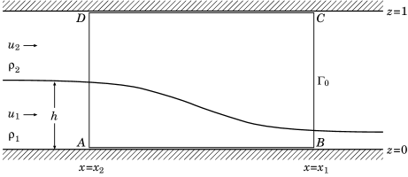
Figure 1: Closed curve $\Gamma_{0}$ fixed on the plane $y=0$.

This curve consists of four segments $AB$, $BC$, $CD$, and $DA$. Segment $AB$ is taken along the upper side of the lower vortex sheet from $x=x_{2}$ to $x=x_{1}$ ($x_{1}$ and $x_{2}$ are arbitrary constants such that $x_{1}>x_{2}$), and $CD$ along the lower side of the upper vortex sheet from $x=x_{1}$ to $x=x_{2}$. Let us introduce here the convention that a zero following a plus or a minus denotes an infinitesimal positive number. Then $AB$ and $CD$ can be written as

$$AB\!:\quad z=\!\mbox{}+0,\quad x_{2}\leq x\leq x_{1};\qquad CD\!:\quad z=1-0,\quad x_{1}\geq x\geq x_{2}.$$

On the other hand, $BC$ is taken vertically upward from $z=\!\mbox{}+0$ to $z=1-0$ at $x=x_{1}$, and $DA$ downward from $z=1-0$ to $z=\!\mbox{}+0$ at $x=x_{2}$. They can also be written as

$$BC\!:\quad x=x_{1},\quad\!\mbox{}+0\leq z\leq 1-0;\qquad DA\!:\quad x=x_{2},\quad 1-0\geq z\geq\!\mbox{}+0.$$

When applied to $\Gamma_{0}$, the conservation law of circulation is expressed by (2.20) with $\Gamma$ replaced by $\Gamma_{0}$. In the following, we consider each term in the expression to deduce one of the four basic laws of the one-dimensional two-layer shallow-water equations.

Let us first discuss the term representing the rate of change of the circulation around $\Gamma_{0}$, i.e. the term on the left-hand side of (2.20). Using (3.3), we have

$$\frac{\mathrm{d}}{\mathrm{d}t_{\ast}}\oint_{\Gamma_{0}}\boldsymbol{u}_{\ast}\cdot\boldsymbol{t}\>\mathrm{d}s_{\ast} =\beta gH\frac{\mathrm{d}}{\mathrm{d}t}\left\{\int_{x_{2}}^{x_{1}}\left(\left.u\right|_{z=\mbox{}+0}-\left.u\right|_{z=1-0}\right)\>\mathrm{d}x\right.$$

$$\quad+\left(\frac{H}{L}\right)^{2}\left.\int_{\!\mbox{}+0}^{1-0}\left(\left.w\right|_{x=x_{1}}-\left.w\right|_{x=x_{2}}\right)\>\mathrm{d}z\right\}.$$ (3.7)

However, since $H/L\ll 1$, the second term in the braces, i.e. the contributions from $BC$ and $DA$, should be neglected. Hence, if (3.5) is used, (3.1.1) can be approximated by

$$\frac{\mathrm{d}}{\mathrm{d}t_{\ast}}\oint_{\Gamma_{0}}\boldsymbol{u}_{\ast}\cdot\boldsymbol{t}\>\mathrm{d}s_{\ast}=\beta gH\frac{\mathrm{d}}{\mathrm{d}t}\int_{x_{2}}^{x_{1}}(u_{1}-u_{2})\>\mathrm{d}x.$$ (3.8)

We next consider the term representing the rate of advection of circulation across $\Gamma_{0}$, i.e. the first term on the right-hand side of (2.20). Since $\boldsymbol{q}_{\ast}=\boldsymbol{u}_{\ast}$ on $\Gamma_{0}$, we can write

$$-\oint_{\Gamma_{0}}\omega_{n\ast}\boldsymbol{q}_{\ast}\cdot\boldsymbol{\nu}\>\mathrm{d}s_{\ast}= -\beta gH\left\{\int_{x_{2}}^{x_{1}}\left(\left.w\frac{\partial u}{\partial z}\right|_{z=\mbox{}+0}-\left.w\frac{\partial u}{\partial z}\right|_{z=1-0}\right)\>\mathrm{d}x\right.$$

$$-\left.\int_{\!\mbox{}+0}^{1-0}\left(\left.u\frac{\partial u}{\partial z}\right|_{x=x_{1}}-\left.u\frac{\partial u}{\partial z}\right|_{x=x_{2}}\right)\>\mathrm{d}z\right\},$$ (3.9)

where we have used (3.3) and (3.4). It should be noted that the first term in the braces represents the advection of circulation across $AB$ and $CD$. Since we have assumed that the upper and lower vortex sheets never separate from the boundaries, this advection of circulation is in fact absent. Thus, using the identity $u\partial u/\partial z=\partial(\frac{1}{2}u^{2})/\partial z$, we obtain

$$-\oint_{\Gamma_{0}}\omega_{n\ast}\boldsymbol{q}_{\ast}\cdot\boldsymbol{\nu}\>\mathrm{d}s_{\ast}=-\beta gH\left[\tfrac{1}{2}u_{1}^{2}-\tfrac{1}{2}u_{2}^{2}\right]_{x=x_{2}}^{x=x_{1}}.$$ (3.10)

Here we have introduced the notation $[\varphi(x,t)]_{x=x_{2}}^{x=x_{1}}=\varphi(x_{1},t)-\varphi(x_{2},t)$.

We can also rewrite the term representing the rate of generation of circulation due to baroclinicity, i.e. the second term on the right-hand side of (2.20), using (3.6) and

$$-\oint_{\Gamma_{0}}\frac{1}{\rho_{\ast}}\nabla p_{\ast}\cdot\boldsymbol{t}\>\mathrm{d}s_{\ast}=-\left(\frac{1}{\rho_{1}}-\frac{1}{\rho_{2}}\right)\left\{\left.p_{\ast}\right|_{x=x_{1},z=h(x_{1},t)}-\left.p_{\ast}\right|_{x=x_{2},z=h(x_{2},t)}\right\}.$$ (3.11)

Indeed, substitution of (3.6) into (3.11) leads to

$$-\oint_{\Gamma_{0}}\frac{1}{\rho_{\ast}}\nabla p_{\ast}\cdot\boldsymbol{t}\>\mathrm{d}s_{\ast}=-\beta gH\left[h-\beta\eta\right]_{x=x_{2}}^{x=x_{1}}.$$ (3.12)

On the other hand, since the external force acting on the fluid is the force of gravity, the term representing the rate of generation of circulation due to the external force, i.e. the third term on the right-hand side of (2.20), vanishes identically:

$$\oint_{\Gamma_{0}}\boldsymbol{f}_{\ast}\cdot\boldsymbol{t}\>\mathrm{d}s_{\ast}=0.$$ (3.13)

Finally, let us consider the term representing the rate of diffusion of circulation across $\Gamma_{0}$, i.e. the last term on the right-hand side of (2.20). Since this term is the line integral along $\Gamma_{0}$ of the viscous force per unit mass, it is seen that the main contributions to the term arise from the points of intersection of $\Gamma_{0}$ and the vortex sheet coincident with the interface. Inside this interfacial vortex sheet, the viscous force per unit mass is expected to be of the same order of magnitude as the inertia force per unit mass:

$$\left|\frac{1}{\rho_{\ast}}\boldsymbol{F}_{\ast}\right|={\it O}\left(\frac{\beta gH}{L}\right),\qquad|y|<\tfrac{1}{2},\quad z=h.$$ (3.14)

Thus, if $\delta$ is the scale characteristic of the dimensional thickness of the interfacial vortex sheet, the magnitude of the term can be estimated as follows:

$$\left|\oint_{\Gamma_{0}}\frac{1}{\rho_{\ast}}\boldsymbol{F}_{\ast}\cdot\boldsymbol{t}\>\mathrm{d}s_{\ast}\right|\leq\oint_{\Gamma_{0}}\left|\frac{1}{\rho_{\ast}}\boldsymbol{F}_{\ast}\right|\>\mathrm{d}s_{\ast}={\it O}\left(\beta gH\frac{\delta}{L}\right).$$ (3.15)

Since $\delta/L\ll 1$, it follows from (3.15) that the term representing the rate of diffusion of circulation across $\Gamma_{0}$ is negligible in comparison with (3.8), (3.10), and (3.12).

As a result, by applying the conservation law of circulation to $\Gamma_{0}$, we obtain

$$\frac{\mathrm{d}}{\mathrm{d}t}\int_{x_{2}}^{x_{1}}(u_{1}-u_{2})\>\mathrm{d}x=-\left[\tfrac{1}{2}u_{1}^{2}-\tfrac{1}{2}u_{2}^{2}+h-\beta\eta\right]_{x=x_{2}}^{x=x_{1}}.$$ (3.16)

What is shown by (3.16) is that the rate of change of the circulation around $\Gamma_{0}$ is equal to the sum of the rate of advection of circulation across $\Gamma_{0}$ and the rate of generation of circulation due to baroclinicity; this is one of the four basic laws of the one-dimensional two-layer shallow-water equations (the ‘fourth’ basic law stated in § 1).

We note here that, in the region enclosed by $\Gamma_{0}$, the surface density of circulation $\omega_{n\ast}$ takes nonzero values only inside the interfacial vortex sheet. Thus it follows that, in the region, circulation is contained only inside the interfacial vortex sheet. This allows us to interpret the above law as describing the balance of circulation for the interfacial vortex sheet. For this reason, the above law is henceforth referred to as the conservation law of circulation for the interfacial vortex sheet.

3.1.2 Conservation law of momentum for the upper and lower layers together

We next consider the volume $\Omega_{0}$ consisting of the upper and lower layers between the planes $x=x_{1}$ and $x=x_{2}$ but out of the vortex sheets on the boundaries:

$$\Omega_{0}\!:\quad x_{2}\leq x\leq x_{1},\quad|y|\leq\tfrac{1}{2}-0,\quad\mbox{}+0\leq z\leq 1-0.$$

By applying the conservation law of momentum in the $x$-direction to $\Omega_{0}$, we have

$$\frac{\mathrm{d}}{\mathrm{d}t}\int_{x_{2}}^{x_{1}}\left\{hu_{1}+(1-\beta)(1-h)u_{2}\right\}\>\mathrm{d}x$$

$$\qquad\quad=-\left[hu_{1}^{2}+(1-\beta)(1-h)u_{2}^{2}+\tfrac{1}{2}h^{2}+(1-\beta)\eta\right]_{x=x_{2}}^{x=x_{1}}.$$ (3.17)

Equation (3.1.2) states that the rate of change of the $x$-component of the momentum in $\Omega_{0}$, represented by the left-hand side, is equal to the sum of the rate of advection of the $x$-component of momentum across the surface enclosing $\Omega_{0}$ and the $x$-component of the total pressure force acting on the surface. This is the conservation law of momentum for the upper and lower layers together.

3.1.3 Conservation laws of mass for the upper layer and for the lower layer

Finally, we consider two other volumes in the channel. One of them, which is denoted by $\Omega_{1}$, is the volume of the lower layer defined by

$$\Omega_{1}\!:\quad x_{2}\leq x\leq x_{1},\quad|y|\leq\tfrac{1}{2}-0,\quad\mbox{}+0\leq z\leq h-0.$$

The other volume, which is denoted by $\Omega_{2}$, is that of the upper layer defined by

$$\Omega_{2}\!:\quad x_{2}\leq x\leq x_{1},\quad|y|\leq\tfrac{1}{2}-0,\quad h+0\leq z\leq 1-0.$$

By applying the conservation law of mass to $\Omega_{1}$, we obtain

$$\frac{\mathrm{d}}{\mathrm{d}t}\int_{x_{2}}^{x_{1}}h\>\mathrm{d}x=-\left[hu_{1}\right]_{x=x_{2}}^{x=x_{1}},$$ (3.18)

i.e. the rate of change of the mass in $\Omega_{1}$ is equal to the rate of advection of mass across the surface enclosing $\Omega_{1}$. Equation (3.18) expresses the conservation law of mass for the lower layer. Similarly, the rate of change of the mass in $\Omega_{2}$ must be equal to the rate of advection of mass across the surface enclosing $\Omega_{2}$:

$$\frac{\mathrm{d}}{\mathrm{d}t}\int_{x_{2}}^{x_{1}}(1-\beta)(1-h)\>\mathrm{d}x=-\left[(1-\beta)(1-h)u_{2}\right]_{x=x_{2}}^{x=x_{1}}.$$ (3.19)

This equation expresses the conservation law of mass for the upper layer.

3.2 Derivation of the equations

We now wish to explain how the one-dimensional two-layer shallow-water equations are derived from the above four basic laws. Suppose first that the variables $u_{1}$, $u_{2}$, $h$, and $\eta$ are all continuously differentiable. Then the four basic laws can be expressed by partial differential equations equivalent to (3.16)–(3.19): the conservation law of circulation for the interfacial vortex sheet can be expressed by

$$\frac{\partial}{\partial t}(u_{1}-u_{2})=-\frac{\partial}{\partial x}(\tfrac{1}{2}u_{1}^{2}-\tfrac{1}{2}u_{2}^{2}+h-\beta\eta);$$ (3.20)

the conservation law of momentum for the upper and lower layers together by

$$\frac{\partial}{\partial t}\left\{hu_{1}+(1-\beta)(1-h)u_{2}\right\}$$

$$\qquad=-\frac{\partial}{\partial x}\left\{hu_{1}^{2}+(1-\beta)(1-h)u_{2}^{2}+\tfrac{1}{2}h^{2}+(1-\beta)\eta\right\};$$ (3.21)

the conservation law of mass for the lower layer by

$$\frac{\partial h}{\partial t}=-\frac{\partial}{\partial x}(hu_{1});$$ (3.22)

and the conservation law of mass for the upper layer by

$$\frac{\partial}{\partial t}\left\{(1-\beta)(1-h)\right\}=-\frac{\partial}{\partial x}\left\{(1-\beta)(1-h)u_{2}\right\}.$$ (3.23)

After some manipulations, we can show that (3.20)–(3.23) yield

$$\left.\begin{array}[]{c}\displaystyle\frac{\partial u_{1}}{\partial t}+u_{1}\frac{\partial u_{1}}{\partial x}=-\frac{\partial h}{\partial x}-(1-\beta)\frac{\partial\eta}{\partial x},\quad\frac{\partial u_{2}}{\partial t}+u_{2}\frac{\partial u_{2}}{\partial x}=-\frac{\partial\eta}{\partial x},\\[10.0pt] \displaystyle\frac{\partial h}{\partial t}=-\frac{\partial}{\partial x}(hu_{1}),\quad\frac{\partial}{\partial t}(1-h)=-\frac{\partial}{\partial x}\left\{(1-h)u_{2}\right\}.\end{array}\right\}$$ (3.24)

This is a well-known form of the one-dimensional two-layer shallow-water equations.

The special case in which the density in the upper layer is much smaller than that in the lower layer, i.e. the case in which $\beta=1-0$, deserves to be considered separately. In this case, the expression (3.2) of the conservation law of momentum for the upper and lower layers together is approximated by

$$\frac{\partial}{\partial t}(hu_{1})=-\frac{\partial}{\partial x}(hu_{1}^{2}+\tfrac{1}{2}h^{2}).$$ (3.25)

As a consequence, from (3.25) and the expression (3.22) of the conservation law of mass for the lower layer, we find the following system of equations for $u_{1}$ and $h$:

$$\frac{\partial u_{1}}{\partial t}+u_{1}\frac{\partial u_{1}}{\partial x}=-\frac{\partial h}{\partial x},\quad\frac{\partial h}{\partial t}=-\frac{\partial}{\partial x}(hu_{1}).$$ (3.26)

This is obviously a form of the one-dimensional single-layer shallow-water equations.

The same system of equations as (3.26) arises in a different context. To show this, we first assume that the thickness of the lower layer is sufficiently small compared with the depth of the channel, i.e. $h\ll 1$. When $h\ll 1$, the expression (3.23) of the conservation law of mass for the upper layer reduces to $\partial u_{2}/\partial x=0$. This allows us to put

$$u_{2}=\mbox{constant}.$$ (3.27)

If, in addition, it is assumed that the density difference between the layers is very small compared with the density in the lower layer, i.e. $\beta=\!\mbox{}+0$, then the expression (3.20) of the conservation law of circulation for the interfacial vortex sheet becomes

$$\frac{\partial u_{1}}{\partial t}=-\frac{\partial}{\partial x}(\tfrac{1}{2}u_{1}^{2}+h).$$ (3.28)

Coupling (3.28) with the expression (3.22) of the conservation law of mass for the lower layer, we obtain the following system of equations:

$$\frac{\partial u_{1}}{\partial t}+u_{1}\frac{\partial u_{1}}{\partial x}=-\frac{\partial h}{\partial x},\quad\frac{\partial h}{\partial t}=-\frac{\partial}{\partial x}(hu_{1}).$$ (3.29)

This is exactly the same system of equations as (3.26).

However, we need to recognize that (3.29) represents, under the condition (3.27), the conservation laws of mass for the lower layer and of circulation for the interfacial vortex sheet. On the other hand, (3.26) represents the conservation laws of mass for the lower layer and of momentum for the upper and lower layers together. From this instance, we can understand that mathematically equivalent systems of partial differential equations do not necessarily represent the same basic physical laws. Though this fact seems to be almost obvious, it is liable to be overlooked.

4 Internal bores

As stated in § 1, within the framework of the one-dimensional two-layer shallow-water equations, an internal bore in a two-fluid system is represented by a shock; the primary objective of this section is to formulate the shock conditions for such a shock. They are shown to be derived from the four basic laws of the equations elucidated in § 3. It must be emphasized, however, that not every shock satisfying the shock conditions represents a bore that can actually exist; if a shock represents a real bore, then the shock satisfies two additional conditions. These conditions, which we call the energy condition and the evolutionary condition, are also discussed. Finally, it is shown that the shock conditions can satisfactorily account for the results of the experiments by Wood & Simpson (1984) on internal bores advancing into two stationary layers of fluid.

4.1 Shock conditions

We consider the same physical situation as that in § 3. However, we now suppose that an internal bore moving parallel to the side boundaries is present in the channel. Except the inside of the bore, the motion of the fluid is assumed to possess the properties described in § 3; the motion changes rapidly inside the bore from the state on one side of the bore to that on the other side. In order to represent properly the motion outside the bore, we use again the dimensionless coordinates $x$, $y$, $z$ and the dimensionless time $t$.

Let $l_{s}$ be the scale of the dimensional distance measured across the bore. We assume that $l_{s}$ is very small compared with the length scale $L$ of the motion outside the bore, i.e. $l_{s}/L\ll 1$. Then the bore may be identified, in the dimensionless coordinate system, with a plane normal to the $x$-axis across which the motion changes discontinuously. We denote the $x$-coordinate of this plane by $x_{s}(t)$.

For $x\neq x_{s}$, the motion of the fluid is specified in terms of the variables $u_{1}$, $u_{2}$, $h$, and $\eta$ introduced in § 3. These variables are discontinuous at $x=x_{s}$, for the motion changes discontinuously there. On the other hand, as we see from the argument in § 3, the set of the variables is determined in each of the infinite intervals $x\leq x_{s}-0$ and $x\geq x_{s}+0$ as a continuous solution of the one-dimensional two-layer shallow-water equations. Thus it follows that, within the framework of the equations, the bore is represented by a shock, i.e. a discontinuity dividing two continuous solutions, located at $x=x_{s}$.

When the bore is represented in this way, the variables $u_{1}$, $u_{2}$, $h$, and $\eta$ at $x=x_{s}-0$ and at $x=x_{s}+0$ need to be related by some conditions. Our aim is to formulate these shock conditions. As explained in the following, each of them is derived from one of the four basic laws of the one-dimensional two-layer shallow-water equations.

First, let us focus our attention on the plane $y=0$, and consider the closed curve $\Gamma_{0}$ introduced in § 3. We suppose that the arbitrary constants $x_{1}$ and $x_{2}$ are so chosen that $x_{1}>x_{s}>x_{2}$. Thus the bore lies between $x=x_{1}$ and $x=x_{2}$, as shown in figure 2.

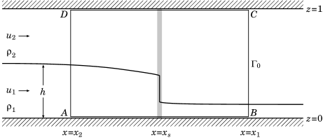
Figure 2: Position of the internal bore relative to $\Gamma_{0}$. The bore is identified with a plane across which the fluid motion changes discontinuously; the grey band shows this plane.

However, we assume that the conservation law of circulation for the interfacial vortex sheet is not altered by the presence of the bore. Then it follows that, while the bore lies between $x=x_{1}$ and $x=x_{2}$, the rate of change of the circulation around $\Gamma_{0}$ is still equal to the sum of the rate of advection of circulation across $\Gamma_{0}$ and the rate of generation of circulation due to baroclinicity. We can formulate a shock condition on the basis of this law. To this end, we must first express the law mathematically. It is expressed by (3.16) if the bore is absent; we wish to examine how this expression should be modified.

The rate of change of the circulation around $\Gamma_{0}$ is now expressed by

$$\frac{\mathrm{d}}{\mathrm{d}t_{\ast}}\oint_{\Gamma_{0}}\boldsymbol{u}_{\ast}\cdot\boldsymbol{t}\>\mathrm{d}s_{\ast} =\beta gH\frac{\mathrm{d}}{\mathrm{d}t}\left\{\int_{x_{2}}^{x_{s}-0}(u_{1}-u_{2})\>\mathrm{d}x+\int_{x_{s}+0}^{x_{1}}(u_{1}-u_{2})\>\mathrm{d}x\right\}$$

$$\quad+\beta gH\frac{\mathrm{d}}{\mathrm{d}t}\int_{x_{s}-0}^{x_{s}+0}\frac{\left.\boldsymbol{u}_{\ast}\right|_{z=\mbox{}+0}-\left.\boldsymbol{u}_{\ast}\right|_{z=1-0}}{(\beta gH)^{\frac{1}{2}}}\cdot\boldsymbol{i}\>\mathrm{d}x$$ (4.1)

in place of (3.8). The last term represents the contribution from the inside of the bore. However, we may expect the velocity there to have the same order of magnitude as that outside the bore: $|\boldsymbol{u}_{\ast}|/(\beta gH)^{\frac{1}{2}}={\it O}(1)$ for $x_{s}-0\leq x\leq x_{s}+0$. Hence the magnitude of the integrand in the term may be estimated to be ${\it O}(1)$. Since the integral is taken over an infinitesimal interval, this estimate reveals that the term is negligible. Accordingly, if the integral on the right-hand side of (3.8) is interpreted as the improper integral

$$\int_{x_{2}}^{x_{1}}(u_{1}-u_{2})\>\mathrm{d}x=\int_{x_{2}}^{x_{s}-0}(u_{1}-u_{2})\>\mathrm{d}x+\int_{x_{s}+0}^{x_{1}}(u_{1}-u_{2})\>\mathrm{d}x,$$ (4.2)

the rate of change of the circulation around $\Gamma_{0}$ is again expressed by (3.8).

On the other hand, the rate of advection of circulation across $\Gamma_{0}$ is now given by

$$-\oint_{\Gamma_{0}}\omega_{n\ast}\boldsymbol{q}_{\ast}\cdot\boldsymbol{\nu}\>\mathrm{d}s_{\ast}= -\beta gH\left[\tfrac{1}{2}u_{1}^{2}-\tfrac{1}{2}u_{2}^{2}\right]_{x=x_{2}}^{x=x_{1}}$$

$$-\beta gH\int_{x_{s}-0}^{x_{s}+0}\frac{\left.\omega_{n\ast}\boldsymbol{u}_{\ast}\right|_{z=1-0}-\left.\omega_{n\ast}\boldsymbol{u}_{\ast}\right|_{z=\mbox{}+0}}{\beta gH/L}\cdot\boldsymbol{k}\>\mathrm{d}x$$ (4.3)

in place of (3.10). The last term in this expression has been introduced to represent the advection of circulation across $\Gamma_{0}$ that occurs inside the bore. However, since the vortex sheets on the upper and lower boundaries have been assumed never to separate from the boundaries, this term vanishes identically. Thus, so long as this assumption is valid, the rate of advection of circulation across $\Gamma_{0}$ is again expressed by (3.10).

Also, it can be shown that the rate of generation of circulation due to baroclinicity is still expressed by (3.12). Thus we reach the conclusion that, while the bore lies between $x=x_{1}$ and $x=x_{2}$, the conservation law of circulation for the interfacial vortex sheet is expressed by (3.16) without any modifications in the form; however, the integral in this expression must be interpreted as the improper integral defined by (4.2).

From this expression of the law, we can now formulate the desired shock condition. If the procedure described by Whitham (1974, § 5.8) is used on (3.16), it is found that the shock representing the bore satisfies the condition

$$-U_{s}\left[u_{1}-u_{2}\right]=-\left[\tfrac{1}{2}u_{1}^{2}-\tfrac{1}{2}u_{2}^{2}+h-\beta\eta\right].$$ (4.4)

Here $U_{s}(t)=\mathrm{d}x_{s}/\mathrm{d}t$ is the velocity of the shock, and $[\varphi(x,t)]=\varphi(x_{s}+0,t)-\varphi(x_{s}-0,t)$ denotes the jump in $\varphi(x,t)$ across the shock. This is the shock condition corresponding to the conservation law of circulation for the interfacial vortex sheet.

Similarly, the remaining shock conditions can be obtained from the other three basic laws of the equations: from the conservation law of momentum for the upper and lower layers together, we obtain

$$-U_{s}\left[hu_{1}+(1-\beta)(1-h)u_{2}\right]=-\left[hu_{1}^{2}+(1-\beta)(1-h)u_{2}^{2}+\tfrac{1}{2}h^{2}+(1-\beta)\eta\right];$$ (4.5)

from the conservation law of mass for the lower layer,

$$-U_{s}\left[h\right]=-\left[hu_{1}\right];$$ (4.6)

and from the conservation law of mass for the upper layer,

$$-U_{s}\left[(1-\beta)(1-h)\right]=-\left[(1-\beta)(1-h)u_{2}\right].$$ (4.7)

The conditions (4.4)–(4.7) constitute the set of shock conditions for the one-dimensional two-layer shallow-water equations (3.24).

It is also possible to write the shock conditions in terms of the relative velocities

$$v_{1}=u_{1}-U_{s},\quad v_{2}=u_{2}-U_{s}.$$ (4.8)

Substituting (4.8) into (4.4)–(4.7) and rearranging the results, we have

$$\left.\begin{array}[]{c}\displaystyle\left[\tfrac{1}{2}v_{1}^{2}-\tfrac{1}{2}v_{2}^{2}+h-\beta\eta\right]=0,\quad\left[hv_{1}\right]=0,\quad\left[(1-\beta)(1-h)v_{2}\right]=0,\\[6.0pt] \displaystyle\left[hv_{1}^{2}+(1-\beta)(1-h)v_{2}^{2}+\tfrac{1}{2}h^{2}+(1-\beta)\eta\right]=0.\end{array}\right\}$$ (4.9)

Let us confirm that the shock conditions (4.4)–(4.7) are consistent with the theory of bores in classical hydraulics. To this end, we now suppose that the density in the upper layer is much smaller than that in the lower layer, i.e. $\beta=1-0$. Then the following set of shock conditions on $u_{1}$ and $h$ can be found:

$$-U_{s}\left[hu_{1}\right]=-\left[hu_{1}^{2}+\tfrac{1}{2}h^{2}\right],\quad-U_{s}\left[h\right]=-\left[hu_{1}\right].$$ (4.10)

The former condition of (4.10) is obtained from the shock condition (4.5) corresponding to the conservation law of momentum for the upper and lower layers together; the latter is the shock condition (4.6) corresponding to the conservation law of mass for the lower layer. The set of shock conditions (4.10) is the one well known in the theory of bores in classical hydraulics (see Whitham 1974, § 13.10).

Note that, when $\beta=1-0$, the variables $u_{1}$ and $h$ are governed in each of the infinite intervals $x\leq x_{s}-0$ and $x\geq x_{s}+0$ by the one-dimensional single-layer shallow-water equations (3.26). This implies that (4.10) is the set of shock conditions for (3.26). Next, let us direct our attention to the system of equations (3.29). This is mathematically the same system of equations as (3.26). However, we can see from the discussion below that (3.29) requires a set of shock conditions different from (4.10).

When deriving (3.29), we assumed that the thickness of the lower layer is sufficiently small compared with the depth of the channel, i.e. $h\ll 1$. If $h\ll 1$, the shock condition (4.7) corresponding to the conservation law of mass for the upper layer reduces to

$$\left[u_{2}\right]=0.$$ (4.11)

Furthermore, it was assumed that the density difference between the layers is very small compared with the density in the lower layer, i.e. $\beta=\!\mbox{}+0$. Let us put again $\beta=\!\mbox{}+0$ and substitute (4.11) into the shock condition (4.4) corresponding to the conservation law of circulation for the interfacial vortex sheet; coupling the result with the shock condition (4.6) corresponding to the conservation law of mass for the lower layer, we obtain

$$-U_{s}\left[u_{1}\right]=-\left[\tfrac{1}{2}u_{1}^{2}+h\right],\quad-U_{s}\left[h\right]=-\left[hu_{1}\right].$$ (4.12)

This is the set of shock conditions for (3.29), and is obviously different from (4.10).

This result may seem somewhat paradoxical since there is no mathematical difference between (3.26) and (3.29). We should realize, however, that each of the shock conditions for a system of equations is derived from one of the basic physical laws that the system represents. As was pointed out at the end of § 3.2, mathematically equivalent systems of equations do not necessarily represent the same basic physical laws. Hence, even though two systems of equations are mathematically equivalent, the sets of shock conditions for the systems may be different. The above result is an instance of this fact.

4.2 Energy condition

It has already been shown that, within the framework of the one-dimensional two-layer shallow-water equations, an internal bore is represented by a shock satisfying the shock conditions (4.4)–(4.7). We should note, however, that there are shocks which satisfy the shock conditions but do not correspond to real bores. In order to exclude such spurious shocks, we need to impose two additional conditions. Our next aim is to elucidate these additional conditions. We first formulate the condition derived from the constraint that mechanical energy cannot be generated inside a bore.

We consider the internal bore in § 4.1, and introduce the following quantity expressed in terms of the relative velocities (4.8):

$$\Phi_{s}(t)=-\left[hv_{1}\left\{\tfrac{1}{2}v_{1}^{2}+h+(1-\beta)\eta\right\}\right]-\left[(1-\beta)(1-h)v_{2}(\tfrac{1}{2}v_{2}^{2}+\eta)\right].$$ (4.13)

It can readily be shown that $\rho_{1}(\beta gH)^{\frac{3}{2}}HW\Phi_{s}$ gives the rate of dissipation of mechanical energy inside the bore. Since mechanical energy cannot be generated inside the bore, we see that the shock representing the bore satisfies the condition

$$\Phi_{s}\geq 0.$$ (4.14)

We call this condition the energy condition. It is to be regarded as a necessary condition for a shock satisfying the shock conditions to represent a real bore.

Now, referring to (4.9), we observe that

$$\left.\left\{hv_{1}+(1-\beta)(1-h)v_{2}\right\}\right|_{x=x_{s}-0}=\left.\left\{hv_{1}+(1-\beta)(1-h)v_{2}\right\}\right|_{x=x_{s}+0}=I_{s}(t).$$ (4.15)

Here $I_{s}$ represents the rate of total advection of mass across the bore. In terms of $I_{s}$, $\Phi_{s}$ can be rewritten, by the use of (4.9), as follows:

$$\Phi_{s}=-I_{s}\left[\tfrac{1}{2}v_{1}^{2}+h+(1-\beta)\eta\right]=-I_{s}\left[\tfrac{1}{2}v_{2}^{2}+\eta\right].$$ (4.16)

This can be seen if we note that the first shock condition in (4.9), which corresponds to the conservation law of circulation for the interfacial vortex sheet, is equivalent to

$$\left[\tfrac{1}{2}v_{1}^{2}+h+(1-\beta)\eta\right]=\left[\tfrac{1}{2}v_{2}^{2}+\eta\right].$$ (4.17)

This expression states that, if viewed by an observer moving with the bore, the changes in total head in the two layers are equal.

In connection with the energy condition, we wish to discuss in the following the rate of dissipation of mechanical energy in each of the two layers.

To this end, we should realize the following fact (see Klemp et al. 1997): the transfer of mechanical energy between the layers may occur inside the bore owing to turbulence. We denote by $\rho_{2}(\beta gH)^{\frac{3}{2}}HW\Psi_{s}(t)$ the rate of this mechanical energy transfer (from the upper layer to the lower layer) perceived by an observer moving with the bore.

Now consider the following quantity:

$$\Phi_{s1}(t)=-\left[hv_{1}\left\{\tfrac{1}{2}v_{1}^{2}+h+(1-\beta)\eta\right\}\right]+(1-\beta)\Psi_{s}.$$ (4.18)

We can see that $\rho_{1}(\beta gH)^{\frac{3}{2}}HW\Phi_{s1}$ gives the rate of dissipation of mechanical energy in the lower layer. The corresponding quantity for the upper layer is

$$\Phi_{s2}(t)=-\left[(1-\beta)(1-h)v_{2}(\tfrac{1}{2}v_{2}^{2}+\eta)\right]-(1-\beta)\Psi_{s}.$$ (4.19)

As is evident from (4.13), the sum of these quantities is equal to $\Phi_{s}$.

It is important to note, however, that there is no means of predicting the value of $\Psi_{s}$. Hence we cannot predict the values of $\Phi_{s1}$ and $\Phi_{s2}$ either. This implies that, within the framework of the one-dimensional two-layer shallow-water equations, the distribution of mechanical energy dissipation inside the bore cannot be predicted in general. (The only exceptional case is the one in which the density in the upper layer is much smaller than that in the lower layer, i.e. the case in which $\beta=1-0$. In this case, we can expect that the mechanical energy dissipation occurs predominantly in the lower layer: on the basis of this expectation, the scale factor $\rho_{2}(\beta gH)^{\frac{3}{2}}HW$ of $\Psi_{s}$ has been chosen.)

4.3 Evolutionary condition

Before starting the discussion of the other additional condition, we need to explain some properties of the one-dimensional two-layer shallow-water equations (3.24).

Note first that, taking linear combinations of (3.24), we can find the following system of equations for $u_{1}$, $u_{2}$, and $h$:

$$\left.\begin{array}[]{c}\displaystyle\frac{\partial}{\partial x}\left\{hu_{1}+(1-h)u_{2}\right\}=0,\quad\frac{\partial h}{\partial t}=-\frac{\partial}{\partial x}(hu_{1}),\\[9.0pt] \displaystyle\frac{\partial u_{1}}{\partial t}+u_{1}\frac{\partial u_{1}}{\partial x}-(1-\beta)\left(\frac{\partial u_{2}}{\partial t}+u_{2}\frac{\partial u_{2}}{\partial x}\right)=-\frac{\partial h}{\partial x}.\end{array}\right\}$$ (4.20)

When this system of equations is hyperbolic, it has three families of characteristics (see e.g. Whitham 1974, § 5.1). One of them is immediately found from the first equation in (4.20). Each characteristic that belongs to this family carries information on the rate of total advection of volume with an infinite characteristic velocity. We denote this family by $C_{vol}$. The characteristic velocities of the other two families are finite. These families correspond to internal waves. We denote by $C_{+}$ the family with the larger characteristic velocity $\lambda_{+}$, and by $C_{-}$ the one with the smaller characteristic velocity $\lambda_{-}$.

Once (4.20) is solved, $\eta$ can be determined from the second equation in (3.24):

$$\frac{\partial\eta}{\partial x}=-\frac{\partial u_{2}}{\partial t}-u_{2}\frac{\partial u_{2}}{\partial x}.$$ (4.21)

When (4.21) is regarded as an equation for $\eta$ alone, it has one family of characteristics. Each characteristic that belongs to this family carries information on $\eta$ with an infinite characteristic velocity. This family of characteristics is denoted by $C_{\eta}$.

Having finished the preparation, we proceed to the discussion of the other additional condition necessary for excluding spurious shocks.

Consider a shock satisfying the shock conditions (4.4)–(4.7). If this shock represents a real bore, then it is evolutionary (see e.g. Landau & Lifshitz 1987, § 88). That the shock is evolutionary means that the following condition is satisfied: there are, at any instant, $N-1$ characteristics leaving the shock and $M-N$ characteristics reaching the shock or moving with the shock. Here $N$ denotes the number of the shock conditions, and $M$ the number of the variables in the shock conditions. We call this condition the evolutionary condition. It also is a necessary condition for a shock satisfying the shock conditions to represent a real bore, and a shock that violates it cannot persist as a single shock.

Let us now examine the evolutionary condition in more detail. First of all, we need to count the number $N$ of the shock conditions and the number $M$ of the variables in the shock conditions. It is apparent that $N$ is four. On the other hand, $M$ is nine: $u_{1}$, $u_{2}$, $h$, and $\eta$ at $x=x_{s}-0$ and at $x=x_{s}+0$, and $U_{s}$. Hence the evolutionary condition can be restated as follows: there are, at any instant, three characteristics leaving the shock and five characteristics reaching the shock or moving with the shock.

It is important to note, however, that the characteristic velocities of $C_{vol}$ and $C_{\eta}$ are infinite. Accordingly, whether a shock is evolutionary or not, two characteristics leaving the shock and two characteristics reaching the shock exist at any instant.

Thus we see that a shock satisfying the shock conditions is evolutionary if and only if either of the following conditions is satisfied at any instant:

$$\left.\begin{array}[]{l}\displaystyle\lambda_{-}-U_{s}<0\leq\lambda_{+}-U_{s}\quad\mbox{at}\quad x=x_{s}-0,\\[2.0pt] \displaystyle\lambda_{-}-U_{s}\leq\lambda_{+}-U_{s}\leq 0\quad\mbox{at}\quad x=x_{s}+0;\end{array}\right\}$$ (4.22)

or

$$\left.\begin{array}[]{l}\displaystyle 0\leq\lambda_{-}-U_{s}\leq\lambda_{+}-U_{s}\quad\mbox{at}\quad x=x_{s}-0,\\[2.0pt] \displaystyle\lambda_{-}-U_{s}\leq 0<\lambda_{+}-U_{s}\quad\mbox{at}\quad x=x_{s}+0.\end{array}\right\}$$ (4.23)

Here $\lambda_{+}-U_{s}$ and $\lambda_{-}-U_{s}$ are the characteristic velocities of $C_{+}$ and $C_{-}$ relative to the shock; they can be calculated from the formulae (see the Appendix)

$$\lambda_{\pm}-U_{s}=\overline{v}\pm\left\{\overline{v}^{2}-\frac{(1-h)v_{1}^{2}+(1-\beta)hv_{2}^{2}-h(1-h)}{(1-\beta)h+(1-h)}\right\}^{\frac{1}{2}},$$ (4.24)

where $v_{1}$ and $v_{2}$ are the relative velocities (4.8), and $\overline{v}$ is defined by

$$\overline{v}=\frac{(1-h)v_{1}+(1-\beta)hv_{2}}{(1-\beta)h+(1-h)}.$$ (4.25)

4.4 Internal bores advancing into two stationary layers of fluid

We have now completed the formulation of the shock conditions for the one-dimensional two-layer shallow-water equations and the additional conditions necessary for excluding spurious shocks. Our remaining task in this section is to confirm that the behaviour of internal bores can really be predicted from the shock conditions (4.4)–(4.7). This task is done especially about bores advancing into two stationary layers of fluid.

Let us consider a shock representing such a bore. In particular, we concentrate on the case in which the density difference between the layers is very small in comparison with the density in the lower layer, i.e. the case in which $\beta=\!\mbox{}+0$. Then the shock conditions (4.9) expressed in terms of the relative velocities (4.8) can be simplified to

$$\left.\begin{array}[]{c}\displaystyle\left[\tfrac{1}{2}v_{1}^{2}-\tfrac{1}{2}v_{2}^{2}+h\right]=0,\quad\left[hv_{1}\right]=0,\quad\left[(1-h)v_{2}\right]=0,\\[6.0pt] \displaystyle\left[hv_{1}^{2}+(1-h)v_{2}^{2}+\tfrac{1}{2}h^{2}+\eta\right]=0.\end{array}\right\}$$ (4.26)

From (4.26), we derive in the following a formula that gives the velocity of the shock as a function of the thicknesses of the lower layer ahead of and behind the shock.

We first assume, without loss of generality, that the shock is advancing in the positive $x$-direction. Since the layers are stationary ahead of the shock, we then have

$$\left.v_{1}\right|_{x=x_{s}+0}=\left.v_{2}\right|_{x=x_{s}+0}=-U_{s}.$$ (4.27)

Next, we introduce the following notation:

$$h_{a}=\left.h\right|_{x=x_{s}+0},\quad h_{b}=\left.h\right|_{x=x_{s}-0},$$ (4.28)

i.e. the thicknesses of the lower layer ahead of and behind the shock are denoted by $h_{a}$ and $h_{b}$ respectively. Substituting (4.27) and (4.28) into the first three shock conditions in (4.26) and solving for $U_{s}$ the resulting system of algebraic equations, we obtain

$$U_{s}=\left\{\frac{2h_{b}^{2}(1-h_{b})^{2}}{h_{a}(1-h_{b})+h_{b}(1-h_{a})}\right\}^{\frac{1}{2}}.$$ (4.29)

Note that (4.29) has been derived from the first three shock conditions in (4.26). This implies that the formula is based on the conservation laws of mass and of circulation; it is independent of the conservation law of momentum.

The energy condition imposes a restriction on the values that $h_{a}$ and $h_{b}$ in (4.29) can take. To find the restriction, we note that $I_{s}$ defined by (4.15) is now given by $-U_{s}<0$. It follows from this fact and (4.16) that the energy condition (4.14) is equivalent to

$$\left[\tfrac{1}{2}v_{1}^{2}+h+\eta\right]\geq 0.$$ (4.30)

This inequality can be expressed, by the use of (4.26)–(4.29), as follows:

$$\frac{-(h_{b}-\tfrac{1}{2})(h_{b}-h_{a})^{3}}{h_{a}(1-h_{b})+h_{b}(1-h_{a})}\geq 0.$$ (4.31)

Thus we see that the energy condition imposes the following restriction on $h_{a}$ and $h_{b}$:

$$h_{a}\leq h_{b}\leq\tfrac{1}{2}\quad\mbox{or}\quad\tfrac{1}{2}\leq h_{b}\leq h_{a}.$$ (4.32)

The values of $h_{a}$ and $h_{b}$ are restricted also by the evolutionary condition. To find the restriction imposed by this condition, we first consider $\overline{v}$ defined by (4.25). It can easily be verified that $\overline{v}$ takes negative values both at $x=x_{s}-0$ and at $x=x_{s}+0$:

$$\left.\overline{v}\right|_{x=x_{s}-0}<0,\quad\left.\overline{v}\right|_{x=x_{s}+0}<0.$$ (4.33)

As we have already seen, the evolutionary condition requires that either (4.22) or (4.23) should hold at any instant. However, on account of (4.33), (4.23) can never be satisfied. Thus, for the shock to be evolutionary, (4.22) needs to be satisfied. Using (4.26)–(4.29), we can show that (4.22) yields the following restriction on $h_{a}$ and $h_{b}$:

$$\left.\begin{array}[]{c}\displaystyle(h_{b}-h_{a})\left\{(6h_{b}^{2}-6h_{b}+2)h_{a}-(3h_{b}^{2}-h_{b})\right\}\geq 0,\\[6.0pt] \displaystyle(h_{b}-h_{a})\left\{2h_{b}^{3}+(2h_{a}-4)h_{b}^{2}+(2h_{a}^{2}-4h_{a}+2)h_{b}-(h_{a}^{2}-h_{a})\right\}\geq 0.\end{array}\right\}$$ (4.34)

We note here that the former part of (4.34) is equivalent to the following restriction:

$$\frac{3h_{b}^{2}-h_{b}}{6h_{b}^{2}-6h_{b}+2}\leq h_{a}\leq h_{b}\quad\mbox{or}\quad h_{b}\leq h_{a}\leq\frac{3h_{b}^{2}-h_{b}}{6h_{b}^{2}-6h_{b}+2}.$$ (4.35)

From this restriction, (4.32) follows immediately. It can readily be demonstrated, on the other hand, that the latter part of (4.34) is automatically satisfied under (4.32). We can therefore conclude that (4.35) is the most stringent restriction on $h_{a}$ and $h_{b}$.

Now, with this restriction on $h_{a}$ and $h_{b}$ in mind, let us examine the validity of (4.29) in the light of the relevant experimental results of Wood & Simpson (1984).

When $h_{a}$ is kept constant in (4.29), $U_{s}$ becomes a function of $h_{b}$ alone. By measuring the velocities of internal bores advancing into two stationary layers of fluid with a small density difference, Wood & Simpson determined, for the values of $h_{a}=0.027$, $0.06$, and $0.12$, the dependence of $U_{s}$ on $h_{b}$. Their results are displayed in figure 3.

Figure 3: Dependence of $U_{s}$ on $h_{b}$ for $h_{a}=0.027$, $0.06$, and $0.12$. The symbols show the experimental results of Wood & Simpson (1984). The curves are obtained from (4.29).

The theoretical curves determined from (4.29) for the three values of $h_{a}$ are also shown for comparison: the curves are drawn for the ranges of $h_{b}$ where (4.35) applies. The agreement between the theory and the experimental results is satisfactorily good in view of the uncertainty in determining $U_{s}$ and $h_{b}$, in particular the latter, from experiment.

Finally, for comparison with (4.29), we add an overview of the similar formulae which follow from the sets of shock conditions proposed in the past mentioned in § 1.

We first consider the set of shock conditions proposed by Yih & Guha (1955). This set of shock conditions is given by (4.9) with its first shock condition replaced by

$$\left[hv_{1}^{2}+\tfrac{1}{2}h^{2}+(1-\beta)h\eta\right]=\tfrac{1}{2}(1-\beta)(\eta_{a}+\eta_{b})(h_{a}-h_{b}),$$ (4.36)

where $\eta_{a}=\eta|_{x=x_{s}+0}$ and $\eta_{b}=\eta|_{x=x_{s}-0}$. Using this set of shock conditions, we can find, in place of (4.29), the following formula:

$$U_{s}=\left\{\frac{h_{b}(1-h_{b})(2-h_{a}-h_{b})(h_{a}+h_{b})}{2(h_{b}^{2}-2h_{a}h_{b}+2h_{a}-h_{a}^{2})}\right\}^{\frac{1}{2}}.$$ (4.37)

Of the two sets of shock conditions suggested by Chu & Baddour (1977) and Wood & Simpson (1984), one is obtained if the first shock condition in (4.9) is replaced by

$$\left[\tfrac{1}{2}v_{2}^{2}+\eta\right]=0.$$ (4.38)

This set of shock conditions yields, in place of (4.29), the following formula:

$$U_{s}=\left\{\frac{h_{b}(1-h_{b})^{2}(h_{a}+h_{b})}{h_{b}^{2}-3h_{a}h_{b}+2h_{a}}\right\}^{\frac{1}{2}}.$$ (4.39)

The other set of shock conditions suggested by Chu & Baddour and Wood & Simpson is obtained if the first shock condition in (4.9) is replaced by

$$\left[\tfrac{1}{2}v_{1}^{2}+h+(1-\beta)\eta\right]=0.$$ (4.40)

From this set of shock conditions, we have, in place of (4.29), the following formula:

$$U_{s}=\left\{\frac{h_{b}^{2}(1-h_{b})(2-h_{a}-h_{b})}{h_{b}^{2}+h_{b}-3h_{a}h_{b}+h_{a}}\right\}^{\frac{1}{2}}.$$ (4.41)

Wood & Simpson (1984) found that (4.37) and (4.39) can predict the velocities of the bores in their experiments when the amplitudes of the bores are small enough; however, it was found at the same time that, when the amplitudes of the bores become large, the predictions from the formulae become unsatisfactory.

Klemp et al. (1997) later showed that the velocities of the bores in the experiments of Wood & Simpson can satisfactorily be predicted by (4.41) irrespective of the amplitudes of the bores. However, as can readily be demonstrated, the set of shock conditions from which (4.41) follows does not allow shocks to exist when the density in the upper layer is much smaller than that in the lower layer, i.e. when $\beta=1-0$; this result is evidently inconsistent with the theory of bores in classical hydraulics.

Accordingly, we can conclude as follows: within the framework of the one-dimensional two-layer shallow-water equations, the set of shock conditions of Yih & Guha and those of Chu & Baddour and Wood & Simpson all must be considered approximate ones that are adequate under specific circumstances.

5 Gravity currents

In this section, we discuss three kinds of gravity currents within the framework of the one-dimensional two-layer shallow-water equations. For each kind of gravity current, we first derive the front conditions, i.e. the boundary conditions to be imposed at the front of the gravity current, from the four basic laws of the equations. We can then find from the front conditions a formula that gives the rate of advance of the gravity current as a function of its depth. After the energy condition and the evolutionary condition for the gravity current are discussed, this velocity formula is derived explicitly for a few special cases; the results are then compared with some empirical or theoretical formulae.

5.1 Gravity currents advancing along a no-slip lower boundary

5.1.1 Front conditions

We consider again the physical situation in § 3. However, it is supposed now that the lower-layer fluid is advancing along the lower boundary as a gravity current. Behind the front of the gravity current, the fluid motion is taken to possess the properties described in § 3. Similarly, sufficiently ahead of the gravity current, the motion is assumed to have the same properties except that the whole depth of the channel is occupied there by the upper-layer fluid. Hence, to represent properly the motion in these regions, we use again the dimensionless coordinates $x$, $y$, $z$ and the dimensionless time $t$. We assume, without loss of generality, that the gravity current is advancing in the positive $x$-direction.

The transition of the motion from the state sufficiently ahead of the gravity current to that behind the front of the current occurs inside a region containing the front. We call this region the frontal region. It is supposed that the motion inside the frontal region is, like the motion outside the region, two-dimensional for $|y|<\tfrac{1}{2}$.

We now assume that, inside the frontal region, the interface between the layers meets the upper side of the lower vortex sheet, i.e. $z=\!\mbox{}+0$, at $x=x_{f}(t)$. Let $l_{f}$ be the scale of the dimensional distance across the frontal region; it is assumed that $l_{f}$ is very small compared with the length scale $L$ of the motion outside the region, i.e. $l_{f}/L\ll 1$. Then, in the dimensionless coordinate system, the frontal region may be idealized into a plane normal to the $x$-axis coincident with $x=x_{f}$. The lower layer is entirely absent ahead of the plane, i.e. for $x\geq x_{f}+0$, but has finite thickness behind it, i.e. for $x\leq x_{f}-0$. Thus the front of the gravity current may be treated as a wall of fluid located at $x=x_{f}$.

Let us next consider the motion in the infinite interval $x\geq x_{f}+0$. The fluid velocity in this interval is again expressed by (3.3); however, since the lower layer is absent, the expression (3.5) for the dimensionless velocity in the $x$-direction reduces to

$$u=u_{2}(x,t),\qquad 0<z<1.$$ (5.1)

The expression (3.6) for the pressure distribution also reduces to

$$p_{\ast}=\rho_{2}\beta gH\eta(x,t)+\rho_{2}gH(1-z),\qquad|y|<\tfrac{1}{2},\quad 0\leq z\leq 1.$$ (5.2)

Thus the motion in the infinite interval $x\geq x_{f}+0$ is specified in terms of the variables $u_{2}$ and $\eta$. These variables are governed by the equations

$$\frac{\partial u_{2}}{\partial x}=0,\quad\frac{\partial\eta}{\partial x}=-\frac{\partial u_{2}}{\partial t}-u_{2}\frac{\partial u_{2}}{\partial x}.$$ (5.3)

On the other hand, the motion in the infinite interval $x\leq x_{f}-0$ is specified in terms of the variables $u_{1}$, $u_{2}$, $h$, and $\eta$ introduced in § 3, and the variables are governed by the one-dimensional two-layer shallow-water equations (3.24). Hence we need to solve (3.24) simultaneously with (5.3) to determine the motion for all $x\neq x_{f}$. To this end, however, it is necessary to know the boundary conditions concerning the variables $u_{1}$, $u_{2}$, $h$, and $\eta$ at $x=x_{f}-0$ and the variables $u_{2}$ and $\eta$ at $x=x_{f}+0$. Our aim is to formulate these boundary conditions which we call the front conditions. They can be obtained, in a way similar to the one to derive the shock conditions, from the four basic laws in § 3.

Let us again focus our attention on the plane $y=0$, and consider the closed curve $\Gamma_{0}$ introduced in § 3. We assume that the arbitrary constants $x_{1}$ and $x_{2}$ are so chosen that $x_{1}>x_{f}>x_{2}$; the frontal region lies between $x=x_{1}$ and $x=x_{2}$, as shown in figure 4.

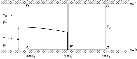
Figure 4: Position of the gravity current relative to $\Gamma_{0}$. The grey band shows the plane which represents the frontal region. The front of the current is contained in this plane, and the point of intersection of the interface and segment $AB$ is denoted by $E$.

In this figure, $E$ denotes the point of intersection of the interface and segment $AB$.

Now let us assume that, despite the special choice of $x_{1}$ and $x_{2}$, the rate of change of the circulation around $\Gamma_{0}$ is still equal to the sum of the rate of advection of circulation across $\Gamma_{0}$ and the rate of generation of circulation due to baroclinicity. Then, from this conservation law of circulation for the interfacial vortex sheet, we can obtain one of the front conditions. To this end, we must first express the law mathematically.

The rate of change of the circulation around $\Gamma_{0}$ can now be written as

$$\frac{\mathrm{d}}{\mathrm{d}t_{\ast}}\oint_{\Gamma_{0}}\boldsymbol{u}_{\ast}\cdot\boldsymbol{t}\>\mathrm{d}s_{\ast} =\beta gH\frac{\mathrm{d}}{\mathrm{d}t}\left\{\int_{x_{2}}^{x_{f}-0}(u_{1}-u_{2})\>\mathrm{d}x+\int_{x_{f}+0}^{x_{1}}(u_{2}-u_{2})\>\mathrm{d}x\right\}$$

$$\quad+\beta gH\frac{\mathrm{d}}{\mathrm{d}t}\int_{x_{f}-0}^{x_{f}+0}\frac{\left.\boldsymbol{u}_{\ast}\right|_{z=\mbox{}+0}-\left.\boldsymbol{u}_{\ast}\right|_{z=1-0}}{(\beta gH)^{\frac{1}{2}}}\cdot\boldsymbol{i}\>\mathrm{d}x.$$ (5.4)

However, it can easily be shown that the last term is negligible. Thus we have

$$\frac{\mathrm{d}}{\mathrm{d}t_{\ast}}\oint_{\Gamma_{0}}\boldsymbol{u}_{\ast}\cdot\boldsymbol{t}\>\mathrm{d}s_{\ast}=\beta gH\frac{\mathrm{d}}{\mathrm{d}t}\int_{x_{2}}^{x_{f}-0}(u_{1}-u_{2})\>\mathrm{d}x.$$ (5.5)

On the other hand, the rate of advection of circulation across $\Gamma_{0}$ can be written as

$$-\oint_{\Gamma_{0}}\omega_{n\ast}\boldsymbol{q}_{\ast}\cdot\boldsymbol{\nu}\>\mathrm{d}s_{\ast} =\beta gH\left.(\tfrac{1}{2}u_{1}^{2}-\tfrac{1}{2}u_{2}^{2})\right|_{x=x_{2}}-\beta gH\left.(\tfrac{1}{2}u_{2}^{2}-\tfrac{1}{2}u_{2}^{2})\right|_{x=x_{1}}$$

$$\quad-\beta gH\int_{x_{f}-0}^{x_{f}+0}\frac{\left.\omega_{n\ast}\boldsymbol{u}_{\ast}\right|_{z=1-0}-\left.\omega_{n\ast}\boldsymbol{u}_{\ast}\right|_{z=\mbox{}+0}}{\beta gH/L}\cdot\boldsymbol{k}\>\mathrm{d}x.$$ (5.6)

The second term on the right-hand side gives the rate of advection of circulation across segment $BC$, but vanishes identically. The last term of (5.1.1) represents the contribution from the advection of circulation across $\Gamma_{0}$ occurring inside the frontal region. It seems reasonable to expect that this term also vanishes, for the upper and lower vortex sheets have been assumed never to separate from the boundaries. However, from the following discussion, it turns out that the term does not vanish contrary to this expectation.

To see this, we first note the following fact: the lower vortex sheet is occupied by the upper-layer fluid for $x\geq x_{f}+0$ but by the lower-layer fluid for $x\leq x_{f}-0$. This implies that, inside the frontal region, the upper-layer fluid in the lower vortex sheet is replaced by the lower-layer fluid as the gravity current advances. As the basis for our discussion, we introduce here a model of this process occurring inside the frontal region: the model is based on the observations of gravity currents by Simpson (1972).

Let us consider the lower vortex sheet inside the frontal region. Ahead of the point of intersection of the interface and the upper side of the vortex sheet, i.e. ahead of point $E$ in figure 4, the vortex sheet is occupied by the upper-layer fluid. As the gravity current advances, $E$ also advances along the upper side of the vortex sheet. However, because of the influence of the no-slip condition at the lower boundary, the upper-layer fluid in the vortex sheet is left behind by $E$ beneath the following lower-layer fluid. In consequence, convective instability arises behind $E$: the upper-layer fluid left beneath the lower-layer fluid rises from the lower vortex sheet, penetrates the lower-layer fluid, and is absorbed into the interfacial vortex sheet; a fraction of the lower-layer fluid, on the other hand, is absorbed into the lower vortex sheet. The upper-layer fluid in the lower vortex sheet is replaced by the lower-layer fluid through this convective instability.

Now let us study the influence of this process on the last term of (5.1.1). We first need to recognize that, when the upper-layer fluid in the lower vortex sheet is left behind by point $E$, circulation also is left behind with the fluid. The amount of the circulation left behind by $E$ per unit time can be calculated from the following formula:

$$-H\int_{0}^{\mbox{}+0}\left.\omega_{n\ast}\right|_{x=x_{f}}\left\{\left.\boldsymbol{q}_{\ast}\right|_{x=x_{f}}-(\beta gH)^{\frac{1}{2}}U_{f}\boldsymbol{i}\right\}\cdot\boldsymbol{i}\>\mathrm{d}z.$$ (5.7)

Here $U_{f}(t)=\mathrm{d}x_{f}/\mathrm{d}t$ is the velocity of $E$, so that $\boldsymbol{q}_{\ast}-(\beta gH)^{\frac{1}{2}}U_{f}\boldsymbol{i}$ gives the dimensional surface velocity relative to $E$; the integral in (5.7) is taken across the lower vortex sheet beneath $E$. Inside the lower vortex sheet, however, $\omega_{n\ast}$ can be approximated by

$$\omega_{n\ast}=-\frac{1}{H}\frac{\partial}{\partial z}(\boldsymbol{u}_{\ast}\cdot\boldsymbol{i}).$$ (5.8)

Substituting (5.8) and $\boldsymbol{q}_{\ast}=\boldsymbol{u}_{\ast}$ into (5.7) and carrying out the integration, we have

$$\tfrac{1}{2}\left\{\left.\boldsymbol{u}_{\ast}\right|_{x=x_{f},z=\mbox{}+0}\cdot\boldsymbol{i}-(\beta gH)^{\frac{1}{2}}U_{f}\right\}^{2}-\tfrac{1}{2}\left\{\left.\boldsymbol{u}_{\ast}\right|_{x=x_{f},z=0}\cdot\boldsymbol{i}-(\beta gH)^{\frac{1}{2}}U_{f}\right\}^{2}.$$ (5.9)

Note that $\boldsymbol{u}_{\ast}|_{x=x_{f},z=\mbox{}+0}$ and $\boldsymbol{u}_{\ast}|_{x=x_{f},z=0}$ are respectively the fluid velocities at $E$ and at the lower boundary. Since $E$ is a material point, these velocities satisfy the conditions

$$\left.\boldsymbol{u}_{\ast}\right|_{x=x_{f},z=\mbox{}+0}=(\beta gH)^{\frac{1}{2}}U_{f}\boldsymbol{i},\quad\left.\boldsymbol{u}_{\ast}\right|_{x=x_{f},z=0}=0,$$ (5.10)

where the latter follows from the no-slip condition at the lower boundary. Hence we see that the amount of the circulation left behind by $E$ per unit time is given by

$$-\beta gH\tfrac{1}{2}U_{f}^{2}.$$ (5.11)

It should be noted here that the circulation left behind by $E$, carried by the upper-layer fluid, rises from the lower vortex sheet and is finally absorbed into the interfacial vortex sheet. As a result, advection of circulation arises inside the frontal region across $\Gamma_{0}$. We can expect that the rate of this advection of circulation across $\Gamma_{0}$ is equal to (5.11):

$$\beta gH\int_{x_{f}-0}^{x_{f}+0}\frac{\left.\omega_{n\ast}\boldsymbol{u}_{\ast}\right|_{z=\mbox{}+0}}{\beta gH/L}\cdot\boldsymbol{k}\>\mathrm{d}x=-\beta gH\tfrac{1}{2}U_{f}^{2}.$$ (5.12)

Note that the lower-layer fluid absorbed into the lower vortex sheet does not contribute to the advection of circulation across $\Gamma_{0}$. This is a consequence of the fact that the fluid enters the vortex sheet from the region outside the vortex sheet where $\omega_{n\ast}=0$.

On the other hand, no circulation leaks from the upper vortex sheet across $\Gamma_{0}$:

$$\beta gH\int_{x_{f}-0}^{x_{f}+0}\frac{\left.\omega_{n\ast}\boldsymbol{u}_{\ast}\right|_{z=1-0}}{\beta gH/L}\cdot\boldsymbol{k}\>\mathrm{d}x=0.$$ (5.13)

Substitution of (5.12) and (5.13) into the last term of (5.1.1) leads to

$$-\oint_{\Gamma_{0}}\omega_{n\ast}\boldsymbol{q}_{\ast}\cdot\boldsymbol{\nu}\>\mathrm{d}s_{\ast}=\beta gH\left.(\tfrac{1}{2}u_{1}^{2}-\tfrac{1}{2}u_{2}^{2})\right|_{x=x_{2}}-\beta gH\tfrac{1}{2}U_{f}^{2}.$$ (5.14)

This is the required expression for the rate of advection of circulation across $\Gamma_{0}$.

Finally, we can write the rate of generation of circulation due to baroclinicity as

$$-\oint_{\Gamma_{0}}\frac{1}{\rho_{\ast}}\nabla p_{\ast}\cdot\boldsymbol{t}\>\mathrm{d}s_{\ast}=-\left(\frac{1}{\rho_{1}}-\frac{1}{\rho_{2}}\right)\left\{\left.p_{\ast}\right|_{x=x_{f},z=\mbox{}+0}-\left.p_{\ast}\right|_{x=x_{2},z=h(x_{2},t)}\right\}.$$ (5.15)

Here $p_{\ast}|_{x=x_{f},z=\mbox{}+0}$ denotes the dimensional pressure at point $E$ in figure 4. As explained below, this pressure can be expressed in terms of the pressure at point $B$ in figure 4.

We first assume that Euler’s equation of motion

$$\frac{\partial\boldsymbol{u}_{\ast}}{\partial t_{\ast}}+\nabla(\tfrac{1}{2}\boldsymbol{u}_{\ast}\cdot\boldsymbol{u}_{\ast})-\boldsymbol{u}_{\ast}\times\boldsymbol{\omega}_{\ast}=-\frac{1}{\rho_{\ast}}\nabla p_{\ast}-g\boldsymbol{k}$$ (5.16)

is valid on segment $EB$ in figure 4, and take the line integral along $EB$ of the equation. Since $EB$ is a streamline, the integral of the third term vanishes. In addition, since $\boldsymbol{k}$ is normal to $EB$, the integral of the last term vanishes as well. Thus we obtain

$$\beta gH\int_{x_{f}}^{x_{1}}\frac{\partial}{\partial t}\left\{\frac{\left.\boldsymbol{u}_{\ast}\right|_{z=\mbox{}+0}}{(\beta gH)^{\frac{1}{2}}}\right\}\cdot\boldsymbol{i}\>\mathrm{d}x+\beta gH\left(\left.\tfrac{1}{2}u_{2}^{2}\right|_{x=x_{1}}-\tfrac{1}{2}U_{f}^{2}\right)$$

$$\qquad\qquad=-\frac{1}{\rho_{2}}\left(\left.p_{\ast}\right|_{x=x_{1},z=\mbox{}+0}-\left.p_{\ast}\right|_{x=x_{f},z=\mbox{}+0}\right).$$ (5.17)

Here we have used the former condition of (5.10) and $\boldsymbol{u}_{\ast}|_{x=x_{1},z=\mbox{}+0}=(\beta gH)^{\frac{1}{2}}u_{2}|_{x=x_{1}}\boldsymbol{i}$. The former of (5.10) also enables us to rewrite the first term of (5.1.1) as

$$\beta gH\frac{\mathrm{d}}{\mathrm{d}t}\int_{x_{f}}^{x_{f}+0}\frac{\left.\boldsymbol{u}_{\ast}\right|_{z=\mbox{}+0}}{(\beta gH)^{\frac{1}{2}}}\cdot\boldsymbol{i}\>\mathrm{d}x+\beta gH\frac{\mathrm{d}}{\mathrm{d}t}\int_{x_{f}+0}^{x_{1}}u_{2}\>\mathrm{d}x+\beta gHU_{f}^{2},$$ (5.18)

where $\boldsymbol{u}_{\ast}|_{z=\mbox{}+0}=(\beta gH)^{\frac{1}{2}}u_{2}\boldsymbol{i}$ has been used for $x\geq x_{f}+0$. However, like the last term of (5.1.1), the first term of (5.18) is negligible. Thus it is seen that (5.1.1) yields

$$\left.p_{\ast}\right|_{x=x_{f},z=\mbox{}+0}=\left.p_{\ast}\right|_{x=x_{1},z=\mbox{}+0}+\rho_{2}\beta gH\left(\left.\tfrac{1}{2}u_{2}^{2}\right|_{x=x_{1}}+\tfrac{1}{2}U_{f}^{2}+\frac{\mathrm{d}}{\mathrm{d}t}\int_{x_{f}+0}^{x_{1}}u_{2}\>\mathrm{d}x\right).$$ (5.19)

This formula expresses the pressure at $E$ in terms of that at $B$.

Substituting (5.19) into (5.15) and then using (3.6) and (5.2), we obtain the following expression for the rate of generation of circulation due to baroclinicity:

$$-\oint_{\Gamma_{0}}\frac{1}{\rho_{\ast}}\nabla p_{\ast}\cdot\boldsymbol{t}\>\mathrm{d}s_{\ast} =\beta gH\left\{\left.(h-\beta\eta)\right|_{x=x_{2}}+\left.\beta\eta\right|_{x=x_{1}}\right\}$$

$$\quad+\beta^{2}gH\left(\left.\tfrac{1}{2}u_{2}^{2}\right|_{x=x_{1}}+\tfrac{1}{2}U_{f}^{2}+\frac{\mathrm{d}}{\mathrm{d}t}\int_{x_{f}+0}^{x_{1}}u_{2}\>\mathrm{d}x\right).$$ (5.20)

Hence, from (5.5), (5.14), and (5.1.1), we see that the conservation law of circulation for the interfacial vortex sheet is expressed by

$$\frac{\mathrm{d}}{\mathrm{d}t}\int_{x_{2}}^{x_{f}-0}(u_{1}-u_{2})\>\mathrm{d}x =\left.(\tfrac{1}{2}u_{1}^{2}-\tfrac{1}{2}u_{2}^{2}+h-\beta\eta)\right|_{x=x_{2}}+\left.\beta\eta\right|_{x=x_{1}}-\tfrac{1}{2}U_{f}^{2}$$

$$\quad+\beta\left(\left.\tfrac{1}{2}u_{2}^{2}\right|_{x=x_{1}}+\tfrac{1}{2}U_{f}^{2}+\frac{\mathrm{d}}{\mathrm{d}t}\int_{x_{f}+0}^{x_{1}}u_{2}\>\mathrm{d}x\right).$$ (5.21)

Note that the third term on the right-hand side of (5.1.1) represents the influence of the lower vortex sheet on the balance of circulation for the interfacial vortex sheet.

Now, applying the procedure described by Whitham (1974, § 5.8) to (5.1.1), we find

$$\left.U_{f}(u_{1}-u_{2})\right|_{x=x_{f}-0} =\left.(\tfrac{1}{2}u_{1}^{2}-\tfrac{1}{2}u_{2}^{2}+h-\beta\eta)\right|_{x=x_{f}-0}+\left.\beta\eta\right|_{x=x_{f}+0}-\tfrac{1}{2}U_{f}^{2}\makebox[10.00002pt]{}$$

$$\quad+\left.\beta\tfrac{1}{2}(u_{2}-U_{f})^{2}\right|_{x=x_{f}+0}.$$ (5.22)

This is the front condition corresponding to the conservation law of circulation for the interfacial vortex sheet. The third term on the right-hand side of (5.1.1) stems from that of (5.1.1), so that the influence of the lower vortex sheet on the balance of circulation for the interfacial vortex sheet is represented by this term.

In contrast, the influence of the lower vortex sheet on the balance of mass and that of momentum can readily be shown to be negligible. Hence the remaining front conditions can be obtained much more easily than (5.1.1): from the conservation law of momentum for the upper and lower layers together, we obtain

$$\left.U_{f}\left\{hu_{1}+(1-\beta)(1-h)u_{2}\right\}\right|_{x=x_{f}-0}-\left.U_{f}(1-\beta)u_{2}\right|_{x=x_{f}+0}$$

$$\quad=\left.\left\{hu_{1}^{2}+(1-\beta)(1-h)u_{2}^{2}+\tfrac{1}{2}h^{2}+(1-\beta)\eta\right\}\right|_{x=x_{f}-0}$$

$$\qquad-\left.\left\{(1-\beta)u_{2}^{2}+(1-\beta)\eta\right\}\right|_{x=x_{f}+0};$$ (5.23)

from the conservation law of mass for the lower layer,

$$\left.U_{f}h\right|_{x=x_{f}-0}=\left.hu_{1}\right|_{x=x_{f}-0};$$ (5.24)

and from the conservation law of mass for the upper layer,

$$\left.U_{f}(1-\beta)(1-h)\right|_{x=x_{f}-0}-U_{f}(1-\beta)$$

$$\quad=\left.(1-\beta)(1-h)u_{2}\right|_{x=x_{f}-0}-\left.(1-\beta)u_{2}\right|_{x=x_{f}+0}.$$ (5.25)

The conditions (5.1.1)–(5.1.1) form the set of front conditions for the gravity current. In (5.1.1)–(5.1.1), $U_{f}$ may be regarded as the rate of advance of the gravity current.

It is convenient to express the front conditions in terms of the relative velocities

$$v_{1}=u_{1}-U_{f},\quad v_{2}=u_{2}-U_{f}.$$ (5.26)

Substituting (5.26) into (5.1.1), we have

$$\left.(\tfrac{1}{2}v_{1}^{2}-\tfrac{1}{2}v_{2}^{2}+h-\beta\eta)\right|_{x=x_{f}-0}+\left.\beta\eta\right|_{x=x_{f}+0}+\left.\beta\tfrac{1}{2}v_{2}^{2}\right|_{x=x_{f}+0}=\tfrac{1}{2}U_{f}^{2}.$$ (5.27)

Here the term on the right-hand side represents the influence of the lower vortex sheet. Also, from (5.1.1)–(5.1.1), we obtain

$$\left.\begin{array}[]{c}\displaystyle\left.hv_{1}\right|_{x=x_{f}-0}=0,\quad\left.(1-\beta)(1-h)v_{2}\right|_{x=x_{f}-0}-\left.(1-\beta)v_{2}\right|_{x=x_{f}+0}=0,\\[6.0pt] \displaystyle\left.\left\{hv_{1}^{2}+(1-\beta)(1-h)v_{2}^{2}+\tfrac{1}{2}h^{2}+(1-\beta)\eta\right\}\right|_{x=x_{f}-0}\\[6.0pt] \displaystyle\mbox{}-\left.\left\{(1-\beta)v_{2}^{2}+(1-\beta)\eta\right\}\right|_{x=x_{f}+0}=0.\makebox[8.6pt]{}\end{array}\right\}$$ (5.28)

In conclusion, it must be stressed that the above front conditions have been obtained on the assumption that the gravity current is advancing relative to the lower boundary: this assumption was explicitly used when we evaluated the influence of the lower vortex sheet on the balance of circulation for the interfacial vortex sheet. Hence it follows that the above front conditions, or (5.1.1) and (5.27) to be more exact, are applicable only to a gravity current advancing relative to a no-slip lower boundary.

5.1.2 Energy condition and evolutionary condition

The gravity current in § 5.1.1 satisfies two additional conditions corresponding to the energy condition and the evolutionary condition stated in § 4 about internal bores. Our next aim is to formulate these additional conditions for the gravity current.

The energy condition for the gravity current can be expressed most concisely in terms of the relative velocity $v_{2}$. We first note that the second front condition in (5.28) yields

$$\left.(1-\beta)(1-h)v_{2}\right|_{x=x_{f}-0}=\left.(1-\beta)v_{2}\right|_{x=x_{f}+0}=I_{f}(t),$$ (5.29)

where $I_{f}$ represents the rate of total advection of mass across the frontal region of the gravity current. We next introduce the following quantity:

$$\Phi_{f}(t)=I_{f}\left\{\left.(\tfrac{1}{2}v_{2}^{2}+\eta)\right|_{x=x_{f}-0}-\left.(\tfrac{1}{2}v_{2}^{2}+\eta)\right|_{x=x_{f}+0}\right\}.$$ (5.30)

In terms of this quantity, the rate of dissipation of mechanical energy inside the frontal region is given by $\rho_{1}(\beta gH)^{\frac{3}{2}}HW\Phi_{f}$. Thus we see that the gravity current satisfies

$$\Phi_{f}\geq 0.$$ (5.31)

This is the energy condition for the gravity current.

Here, as in § 4.2, a remark needs to be made on the distribution of mechanical energy dissipation inside the frontal region. The dissipation of mechanical energy may arise, on account of turbulence, both in the gravity current and in the ambient fluid; however, we cannot predict the distribution of the dissipation, for it is impossible to predict the rate of transfer of mechanical energy between the gravity current and the ambient fluid.

Let us next consider the evolutionary condition for the gravity current. This condition can be stated as follows: there are, at any instant, $N-1$ characteristics leaving the front of the gravity current and $M-N$ characteristics reaching the front or moving with the front. Here $N$ is the number of the front conditions, and $M$ the number of the variables in the front conditions. Apparently, $N$ is four. On the other hand, $M$ is seven: $u_{1}$, $u_{2}$, $h$, and $\eta$ at $x=x_{f}-0$, $u_{2}$ and $\eta$ at $x=x_{f}+0$, and $U_{f}$.

To express mathematically the evolutionary condition for the gravity current, we now recall that the fluid motion is governed by the one-dimensional two-layer shallow-water equations (3.24) for $x\leq x_{f}-0$. As we have seen in § 4.3, the system (3.24) has the four families of characteristics $C_{+}$, $C_{-}$, $C_{vol}$, and $C_{\eta}$. For $x\geq x_{f}+0$, however, the motion is governed by the equations (5.3). It can easily be seen that the system (5.3) has the two families of characteristics $C_{vol}$ and $C_{\eta}$. Accordingly, a discussion similar to that in § 4.3 leads us to the conclusion that the evolutionary condition is equivalent to

$$\lambda_{-}-U_{f}<0\leq\lambda_{+}-U_{f}\quad\mbox{at}\quad x=x_{f}-0,$$ (5.32)

where $\lambda_{+}-U_{f}$ and $\lambda_{-}-U_{f}$ denote the characteristic velocities of $C_{+}$ and $C_{-}$ relative to the front of the gravity current. We can calculate the relative characteristic velocities again from (4.24) and (4.25) by replacing $U_{s}$ in (4.24) with $U_{f}$: we must, of course, take $v_{1}$ and $v_{2}$ in the formulae as the relative velocities defined by (5.26).

5.1.3 Velocity formula

The front conditions (5.1.1)–(5.1.1) for the gravity current in § 5.1.1 may be considered a system of four algebraic equations for the following seven variables: $u_{1}$, $u_{2}$, $h$, and $\eta$ at $x=x_{f}-0$, $u_{2}$ and $\eta$ at $x=x_{f}+0$, and $U_{f}$. Hence, if we are given the values of the two variables at $x=x_{f}+0$, $U_{f}$ can be determined from the front conditions as a function of one of the four variables at $x=x_{f}-0$. In the following, we derive specifically a formula that gives $U_{f}$ as a function of $h$ at $x=x_{f}-0$, and then compare it with some empirical formulae so as to confirm the validity of the front conditions.

To derive this velocity formula, we first need to determine $u_{2}$ and $\eta$ for $x\geq x_{f}+0$. It is seen from (5.3) that these variables must take constant values for $x\geq x_{f}+0$. Thus, if the constant value of $\eta$ is put equal to zero without loss of generality, we have

$$u_{2}=U_{\infty},\quad\eta=0,\qquad x\geq x_{f}+0,$$ (5.33)

where $U_{\infty}$ denotes the value of $u_{2}$ at $x=\infty$.

Consider now the front conditions (5.27) and (5.28) expressed in terms of the relative velocities (5.26). The parameter $\beta$ in the conditions can take any value between $\!\mbox{}+0$ and $1-0$, but we assume particularly that the density in the gravity current is almost equal to the ambient density, i.e. $\beta=\!\mbox{}+0$. Then (5.27) reduces to

$$\left.(\tfrac{1}{2}v_{1}^{2}-\tfrac{1}{2}v_{2}^{2}+h)\right|_{x=x_{f}-0}=\tfrac{1}{2}U_{f}^{2}.$$ (5.34)

The conditions (5.28) also reduce to

$$\left.\begin{array}[]{c}\displaystyle\left.hv_{1}\right|_{x=x_{f}-0}=0,\quad\left.(1-h)v_{2}\right|_{x=x_{f}-0}=U_{\infty}-U_{f},\\[6.0pt] \displaystyle\left.\left\{hv_{1}^{2}+(1-h)v_{2}^{2}+\tfrac{1}{2}h^{2}+\eta\right\}\right|_{x=x_{f}-0}=(U_{\infty}-U_{f})^{2}.\end{array}\right\}$$ (5.35)

Here we have used the following conditions obtained from (5.26) and (5.33):

$$\left.v_{2}\right|_{x=x_{f}+0}=U_{\infty}-U_{f},\quad\left.\eta\right|_{x=x_{f}+0}=0.$$ (5.36)

If (5.34) and the first two front conditions in (5.35) are used, we can determine $U_{f}$ as a function of $h$ at $x=x_{f}-0$. Introducing the notation

$$h_{b}=\left.h\right|_{x=x_{f}-0},$$ (5.37)

we can express the result as follows:

$$U_{f}=\frac{U_{\infty}}{1+(1-h_{b})^{2}}+\frac{(1-h_{b})\left\{2h_{b}+2h_{b}(1-h_{b})^{2}-U_{\infty}^{2}\right\}^{\frac{1}{2}}}{1+(1-h_{b})^{2}}.$$ (5.38)

This is the required velocity formula under the condition $\beta=\!\mbox{}+0$.

It deserves attention that (5.38) has been obtained from (5.34) and the first two front conditions in (5.35). We see from this fact that (5.38) is based on the conservation laws of mass and of circulation; it is independent of the conservation law of momentum.

We should also note that (5.38) is valid only when $U_{f}>0$. This can be seen from the fact stated at the end of § 5.1.1: the front condition (5.27), from which (5.34) follows, is valid only when the gravity current is advancing relative to the lower boundary.

Now let the ambient fluid be stationary sufficiently ahead of the gravity current. The velocity formula (5.38) then reduces to

$$U_{f}=(1-h_{b})\left\{\frac{2h_{b}}{1+(1-h_{b})^{2}}\right\}^{\frac{1}{2}},$$ (5.39)

since $U_{\infty}=0$. For a while, we concentrate on the discussion of (5.39).

The evolutionary condition (5.32) places the following restriction on $h_{b}$ in (5.39):

$$\!\mbox{}+0\leq h_{b}\leq 0.404.$$ (5.40)

We can also verify that the energy condition (5.31) holds over the range (5.40).

Figure 5 shows a graph of (5.39): it is drawn for the range (5.40).

Figure 5: The solid line shows a graph of (5.39). Also shown for comparison is a graph of (5.55): this formula applies when the no-slip condition at the lower boundary is relaxed.

As we can see from the graph, $U_{f}$ takes the maximum value when $h_{b}=0.404$. This maximum value is

$$U_{f}=0.460.$$ (5.41)

Note also that, when $h_{b}=0.404$, the gravity current is marginally evolutionary:

$$\lambda_{-}<U_{f}=\lambda_{+}\quad\mbox{at}\quad x=x_{f}-0.$$ (5.42)

Klemp et al. (1994) showed that a marginally evolutionary gravity current is formed in what is called a lock-exchange experiment. Thus it is expected that the rate of advance of the gravity current formed in a lock-exchange experiment is given by (5.41).

An empirical formula that gives the rate of advance of the gravity current formed in a lock-exchange experiment can be found in the monograph of Yih (1965, p. 136):

$$U_{f}=0.67(2-\beta)^{-\frac{1}{2}}.$$ (5.43)

Though (5.43) contains the parameter $\beta$, it was in fact obtained for very small values of $\beta$. Hence we may safely put $\beta=\!\mbox{}+0$ in (5.43). Then we have

$$U_{f}=0.47.$$ (5.44)

As has been expected, (5.44) agrees well with (5.41).

On the other hand, as $h_{b}\rightarrow\!\mbox{}+0$, (5.39) asymptotically approaches

$$U_{f}=h_{b}^{\frac{1}{2}}.$$ (5.45)

This asymptotic behaviour of (5.39) coincides with that of the empirical formula

$$U_{f}=\left\{\frac{h_{b}(1-h_{b})(2-h_{b})}{2(1+h_{b})}\right\}^{\frac{1}{2}}$$ (5.46)

proposed by Rottman & Simpson (1983) and shown to be adequate when $h_{b}$ is small.

Having considered the special case in which $U_{\infty}=0$, we now return to the discussion of the original velocity formula (5.38) to examine the dependence of $U_{f}$ on $U_{\infty}$.

We should first recall that $U_{f}$ given by (5.38) must satisfy the underlying assumption $U_{f}>0$. It is seen from (5.38) that, for $U_{f}>0$ to be fulfilled by some value of $h_{b}$,

$$-({\textstyle\frac{2}{3}})^{\frac{3}{2}}<U_{\infty}<2^{\frac{1}{2}}$$ (5.47)

needs to be satisfied. We may interpret (5.47) as a necessary condition for the existence of a gravity current advancing relative to a no-slip lower boundary.

When $h_{b}$ is assumed to be constant in (5.38), $U_{f}$ may be considered a function of $U_{\infty}$ alone. If $U_{\infty}^{2}\ll 2h_{b}\{1+(1-h_{b})^{2}\}$ in addition, then (5.38) is approximated by

$$U_{f}=\frac{U_{\infty}}{1+(1-h_{b})^{2}}+(1-h_{b})\left\{\frac{2h_{b}}{1+(1-h_{b})^{2}}\right\}^{\frac{1}{2}}.$$ (5.48)

It is of interest to compare this approximate velocity formula and the empirical formula obtained by Simpson & Britter (1980) stated below.

Simpson & Britter examined the dependence of $U_{f}$ on $U_{\infty}$ by experiment. They tried to express $U_{f}$, as a function of $U_{\infty}$, in the form

$$U_{f}=aU_{\infty}+bh_{b}^{\frac{1}{2}},$$ (5.49)

and found that $(a,b)=(0.62,0.91)$ for $0.15<h_{b}<0.25$. However, if we compare (5.48) and (5.49), it is seen that $a$ and $b$ in (5.49) can be written as

$$a=\frac{1}{1+(1-h_{b})^{2}},\quad b=(1-h_{b})\left\{\frac{2}{1+(1-h_{b})^{2}}\right\}^{\frac{1}{2}}.$$ (5.50)

When $h_{b}=0.2$, for example, (5.50) predicts that $(a,b)=(0.61,0.88)$. This prediction is in good agreement with the above result of Simpson & Britter.

Finally, we wish to discuss briefly the case in which the density in the gravity current is much larger than the ambient density, i.e. the case in which $\beta=1-0$.

To this end, we need to return to the consideration of the front conditions (5.27) and (5.28). It can readily be seen from (5.27) and (5.28) that, when $\beta=1-0$, $U_{f}$ cannot be determined as a function of $h$ at $x=x_{f}-0$. Instead, the conditions require that

$$\left.h\right|_{x=x_{f}-0}=\!\mbox{}+0.$$ (5.51)

Thus, when $\beta=1-0$, the front of the gravity current cannot take the form of a wall of fluid. This is a fact well known in classical hydraulics (see Whitham 1974, § 13.10).

5.2 Gravity currents advancing along a lower boundary with slip

5.2.1 Front conditions

Let us consider again the gravity current in § 5.1.1. However, we now assume that the upper- and lower-layer fluids are allowed to slip at the lower boundary. Accordingly, the vortex sheet on the lower boundary is now entirely absent.

The absence of the lower vortex sheet affects the front condition corresponding to the conservation law of circulation for the interfacial vortex sheet: the term representing the influence of the vortex sheet vanishes. For example, (5.27) now becomes

$$\left.(\tfrac{1}{2}v_{1}^{2}-\tfrac{1}{2}v_{2}^{2}+h-\beta\eta)\right|_{x=x_{f}-0}+\left.\beta\eta\right|_{x=x_{f}+0}+\left.\beta\tfrac{1}{2}v_{2}^{2}\right|_{x=x_{f}+0}=0.$$ (5.52)

In contrast, the remaining front conditions (5.28) are unaltered.

5.2.2 Energy condition and evolutionary condition

The energy condition and the evolutionary condition for the gravity current in § 5.1.1 are unaffected by the absence of the lower vortex sheet. Hence the energy condition can be expressed by (5.31) as before, and the evolutionary condition by (5.32).

5.2.3 Velocity formula

Now let us derive the velocity formula from the front conditions stated in § 5.2.1. The derivation is to be carried out for two special cases separately.

The first case is the one in which the density in the gravity current is almost equal to the ambient density, i.e. the case in which $\beta=\!\mbox{}+0$. In this case, as explained in § 5.1.3, the conditions (5.28) reduce to (5.35). On the other hand, (5.52) becomes

$$\left.(\tfrac{1}{2}v_{1}^{2}-\tfrac{1}{2}v_{2}^{2}+h)\right|_{x=x_{f}-0}=0.$$ (5.53)

From (5.53) and the first two front conditions in (5.35), we obtain

$$U_{f}=U_{\infty}+(1-h_{b})(2h_{b})^{\frac{1}{2}}.$$ (5.54)

Note that (5.54) expresses $U_{f}$ as the sum of $U_{\infty}$ and a term independent of $U_{\infty}$. This implies that, in the absence of the lower vortex sheet, the rate of advance of the gravity current relative to the ambient fluid is independent of the velocity of the ambient fluid.

Let us now suppose that $U_{\infty}=0$. Then (5.54) reduces to

$$U_{f}=(1-h_{b})(2h_{b})^{\frac{1}{2}}.$$ (5.55)

The evolutionary condition (5.32) requires that $h_{b}$ in (5.55) should lie in the range

$$\!\mbox{}+0\leq h_{b}\leq{\textstyle\frac{1}{3}}.$$ (5.56)

The energy condition (5.31) is automatically satisfied for this range of $h_{b}$.

The formula (5.55) should be compared with (5.39) derived in § 5.1.3 in the presence of the lower vortex sheet. To this end, we have included in figure 5 a graph of (5.55) for the range (5.56). Comparing the graph with that of (5.39), we see that, for any value of $h_{b}$ in the range (5.56), (5.55) gives a larger value of $U_{f}$ than (5.39). It is also seen from the graph that, when $h_{b}=\frac{1}{3}$, (5.55) gives the following maximum value of $U_{f}$:

$$U_{f}=({\textstyle\frac{2}{3}})^{\frac{3}{2}}=0.544.$$ (5.57)

This is again larger than the maximum value (5.41) obtained from (5.39). These results allow us to say that the gravity current is retarded by friction at the lower boundary. It must be emphasized, however, that the retardation of the gravity current is not directly caused by the frictional force exerted by the lower boundary; the retardation is, in fact, due to the advection of circulation from the lower vortex sheet elucidated in § 5.1.1.

It is also of interest to compare (5.55) with (4.29) derived in § 4.4 for an internal bore advancing into two stationary layers of fluid. Comparing the formulae, we observe that, if $U_{s}$ in (4.29) is identified with $U_{f}$, (5.55) is obtained from (4.29) when $h_{a}\ll h_{b}$. Hence the gravity current may be regarded as an extreme form of the internal bore considered in § 4.4, though this is not allowed when the lower vortex sheet is present.

Now let us turn to the consideration of the second case. This case is the one in which the ambient fluid is much deeper than the gravity current, i.e. the case in which $h\ll 1$ for $x\leq x_{f}-0$. Though the value of $\beta$ is left unspecified, it is assumed that $1-\beta$ is not very small. To derive the velocity formula, we first introduce the approximation

$$\left.(1-h)\right|_{x=x_{f}-0}=1.$$ (5.58)

If this approximation and (5.36) are used, (5.28) can be simplified to

$$\left.\begin{array}[]{c}\displaystyle\left.hv_{1}\right|_{x=x_{f}-0}=0,\quad\left.v_{2}\right|_{x=x_{f}-0}=U_{\infty}-U_{f},\\[6.0pt] \displaystyle\left.\left\{hv_{1}^{2}+(1-\beta)v_{2}^{2}+\tfrac{1}{2}h^{2}+(1-\beta)\eta\right\}\right|_{x=x_{f}-0}=(1-\beta)(U_{\infty}-U_{f})^{2}.\end{array}\right\}$$ (5.59)

On the other hand, substitution of (5.36) into (5.52) leads to

$$\left.(\tfrac{1}{2}v_{1}^{2}-\tfrac{1}{2}v_{2}^{2}+h-\beta\eta)\right|_{x=x_{f}-0}=-\beta\tfrac{1}{2}(U_{\infty}-U_{f})^{2}.$$ (5.60)

If $v_{1}$, $v_{2}$, and $\eta$ at $x=x_{f}-0$ are eliminated from (5.59) and (5.60), we have

$$(1-\beta)^{2}\tfrac{1}{2}(U_{\infty}-U_{f})^{2}=\left\{(1-\beta)+\tfrac{1}{2}\beta h_{b}\right\}h_{b}.$$ (5.61)

Since $1-\beta$ is not very small, we can assume that $\tfrac{1}{2}\beta h_{b}\ll 1-\beta$; (5.61) then yields

$$U_{f}=U_{\infty}+\left(\frac{2h_{b}}{1-\beta}\right)^{\frac{1}{2}}.$$ (5.62)

We can easily see that (5.62) is the velocity formula obtained by von Kármán (1940), on the basis of Bernoulli’s theorem, for a gravity current of the same kind. Hence, while von Kármán’s argument leading to his formula was later shown to be invalid (Benjamin 1968), his formula itself is applicable when the lower vortex sheet is absent.

When $\beta=\!\mbox{}+0$, von Kármán’s velocity formula (5.62) reduces to

$$U_{f}=U_{\infty}+(2h_{b})^{\frac{1}{2}}.$$ (5.63)

On the other hand, (5.63) is also obtained from (5.54) when $h_{b}\ll 1$. Here we recall that (5.54) was derived from the front conditions based on the conservation laws of mass and of circulation. Thus we see that, when $\beta=\!\mbox{}+0$, i.e. when the Boussinesq approximation is adequate, von Kármán’s formula can be derived on the basis of the conservation laws of mass and of circulation. This is a fact pointed out by Rotunno et al. (1988).

5.3 Gravity currents advancing along a no-slip upper boundary

5.3.1 Front conditions

As in § 5.1.1, we consider the physical situation in § 3. However, in contrast to § 5.1.1, the upper-layer fluid is assumed to be advancing along the upper boundary as a gravity current. The front of the current is again identified with an inverted wall of fluid which is located at $x=x_{f}$ and is contained in the plane representing the frontal region.

In § 5.1.1, the motion in the infinite interval $x\leq x_{f}-0$ was considered to be specified in terms of the variables $u_{1}$, $u_{2}$, $h$, and $\eta$ introduced in § 3. However, it is preferable for our present purpose to employ, instead of $\eta$, the new variable $\zeta(x,t)$ which is so defined that $\rho_{1}\beta gH\zeta$ gives the pressure at the lower boundary for $|y|<\tfrac{1}{2}$. Thus we henceforth assume that the motion in the infinite interval $x\leq x_{f}-0$ is specified in terms of $u_{1}$, $u_{2}$, $h$, and $\zeta$. The pressure distribution in this interval is expressed in terms of $\zeta$ by

$$p_{\ast}=\left\{\begin{array}[]{lll}\rho_{1}\beta gH\zeta-\rho_{1}gHz,&|y|<\tfrac{1}{2},&0\leq z\leq h,\\[2.0pt] \rho_{1}\beta gH\zeta-\rho_{1}gHh-\rho_{2}gH(z-h),&|y|<\tfrac{1}{2},&h\leq z\leq 1.\end{array}\right.$$ (5.64)

As for the motion in the infinite interval $x\geq x_{f}+0$, it can be specified in terms of $u_{1}$ and $\zeta$. Indeed, in this interval, the dimensionless velocity $u$ in (3.3) is given by

$$u=u_{1}(x,t),\qquad 0<z<1.$$ (5.65)

Now, by an argument similar to that in § 5.1.1, we can find the front conditions. The one corresponding to the conservation law of circulation for the interfacial vortex sheet is expressed, in terms of the relative velocities (5.26), by

$$\left.\left\{\tfrac{1}{2}v_{1}^{2}-\tfrac{1}{2}v_{2}^{2}-\frac{(1-h)+\beta\zeta}{1-\beta}\right\}\right|_{x=x_{f}-0}+\left.\frac{\beta\zeta}{1-\beta}\right|_{x=x_{f}+0}+\left.\frac{\beta\tfrac{1}{2}v_{1}^{2}}{1-\beta}\right|_{x=x_{f}+0}=-\tfrac{1}{2}U_{f}^{2}.$$ (5.66)

Here the term on the right-hand side represents the influence of the upper vortex sheet. The remaining front conditions are as follows:

$$\left.\begin{array}[]{c}\displaystyle\left.hv_{1}\right|_{x=x_{f}-0}-\left.v_{1}\right|_{x=x_{f}+0}=0,\quad\left.(1-\beta)(1-h)v_{2}\right|_{x=x_{f}-0}=0,\\[6.0pt] \displaystyle\left.\left\{hv_{1}^{2}+(1-\beta)(1-h)v_{2}^{2}+\tfrac{1}{2}(1-h)^{2}+\zeta\right\}\right|_{x=x_{f}-0}-\left.(v_{1}^{2}+\zeta)\right|_{x=x_{f}+0}=0.\end{array}\right\}$$ (5.67)

5.3.2 Energy condition and evolutionary condition

Let us formulate the energy condition for the gravity current in § 5.3.1. In view of the first front condition in (5.67), we can write

$$\left.hv_{1}\right|_{x=x_{f}-0}=\left.v_{1}\right|_{x=x_{f}+0}=I_{f}(t).$$ (5.68)

The energy condition is expressed by (5.31) if we define $\Phi_{f}$ as follows:

$$\Phi_{f}(t)=I_{f}\left\{\left.(\tfrac{1}{2}v_{1}^{2}+\zeta)\right|_{x=x_{f}-0}-\left.(\tfrac{1}{2}v_{1}^{2}+\zeta)\right|_{x=x_{f}+0}\right\}.$$ (5.69)

Also, the evolutionary condition for the gravity current is expressed by (5.32).

5.3.3 Velocity formula

To find the velocity formula for the gravity current in § 5.3.1, we first put

$$u_{1}=U_{\infty},\quad\zeta=0,\qquad x\geq x_{f}+0.$$ (5.70)

The velocity formula can now be derived from (5.66) and (5.67). Let us first consider, as in § 5.1.3, the case in which the density in the gravity current is almost equal to the ambient density, i.e. the case in which $\beta=\!\mbox{}+0$. In this case, (5.66) reduces to

$$\left.\left\{\tfrac{1}{2}v_{1}^{2}-\tfrac{1}{2}v_{2}^{2}-(1-h)\right\}\right|_{x=x_{f}-0}=-\tfrac{1}{2}U_{f}^{2}.$$ (5.71)

Using this together with (5.67), we obtain the following formula:

$$U_{f}=\frac{U_{\infty}}{1+h_{b}^{2}}+\frac{h_{b}\left\{2(1-h_{b})+2h_{b}^{2}(1-h_{b})-U_{\infty}^{2}\right\}^{\frac{1}{2}}}{1+h_{b}^{2}}.$$ (5.72)

Comparing this formula with (5.38) in § 5.1.3, we observe that (5.72) is also obtained from (5.38) when $h_{b}$ in (5.38) is replaced by $1-h_{b}$. It follows from this fact that, when $\beta=\!\mbox{}+0$, the rate of advance of the gravity current is equal to that of a gravity current with the same dimensionless depth advancing along a no-slip lower boundary.

We next consider the case in which the density in the gravity current is much smaller than the ambient density, i.e. the case in which $\beta=1-0$. In this case, (5.66) yields

$$-\left.\left\{(1-h)+\zeta\right\}\right|_{x=x_{f}-0}+\tfrac{1}{2}(U_{\infty}-U_{f})^{2}=0.$$ (5.73)

From this and (5.67), the velocity formula is obtained in the form

$$U_{f}=U_{\infty}+\left\{\frac{h_{b}(1+h_{b})(1-h_{b})}{2-h_{b}}\right\}^{\frac{1}{2}}.$$ (5.74)

In deriving (5.74), we used (5.73). While (5.73) was obtained from (5.66), it does not contain the term representing the influence of the upper vortex sheet. This implies that the presence of the upper vortex sheet is inessential for (5.74) to be valid; (5.74) applies even if the upper- and lower-layer fluids are allowed to slip at the upper boundary. This result is in accord with the fact that (5.74) is the velocity formula derived by Benjamin (1968) for a gravity current of the same kind on the basis of inviscid-fluid theory.

It can readily be shown, however, that (5.74) is obtained only when the density in the gravity current is much smaller than the ambient density. We can therefore conclude as follows: within the framework of the one-dimensional two-layer shallow-water equations, Benjamin’s formula applies only to a gravity current whose density is much smaller than the ambient density, i.e. a gravity current identifiable with a ‘cavity’.

6 Discussion

A unified theory of internal bores and gravity currents has been developed within the framework of the one-dimensional two-layer shallow-water equations, and the validity of the theory has been confirmed in the light of some empirical facts. It should be borne in mind, however, that the theory is based on several assumptions. Hence the theory is not directly applicable to internal bores and gravity currents which violate the assumptions. In this section, we discuss two examples of such internal bores and gravity currents.

6.1 Internal hydraulic jumps

An internal hydraulic jump is defined, in this paper, as a steady and stationary internal bore with the following property: the lower-layer fluid crosses the bore from the side on which the level of the interface is lower to the side on which it is higher. Our purpose is to examine how an internal hydraulic jump can be treated within the framework of the one-dimensional two-layer shallow-water equations.

It may seem, at first sight, that an internal hydraulic jump can be treated as a shock satisfying the shock conditions (4.4)–(4.7) with $U_{s}$ in them put equal to zero. We should note, however, that (4.4)–(4.7) were derived on the assumption that the vortex sheet on a boundary never separates from the boundary. Hence (4.4)–(4.7) lose their basis if this assumption is invalid. In fact, an internal hydraulic jump invalidates this assumption.

To show this, we first note that the lower-layer fluid experiences an abrupt thickening of the lower layer when it crosses an internal hydraulic jump. Thus the lower-layer fluid is decelerated rapidly inside an internal hydraulic jump. However, it is well known that, when a steady flow along a rigid boundary is decelerated rapidly in the direction of the flow, the vortex sheet on the boundary separates from the boundary (see e.g. Batchelor 1967, § 5.10). Hence we can conclude that, inside an internal hydraulic jump, separation of the vortex sheet on the lower boundary occurs inevitably.

We must take this separation into account in dealing with an internal hydraulic jump within the framework of the one-dimensional two-layer shallow-water equations. On the other hand, within the framework of the equations, separation of a vortex sheet cannot be treated directly. Hence, to resolve this difficulty, we introduce a model of an internal hydraulic jump in which the separation is represented in a indirect manner.

In this model, it is supposed that the vortex sheet on the lower boundary is attached to the boundary everywhere inside the jump. Instead, to represent the separation of the vortex sheet, we assume the following process to take place somewhere inside the jump: the fluid in the vortex sheet leaks from the vortex sheet; it then rises through the lower layer and is absorbed into the interfacial vortex sheet. In compensation for this process, a fraction of the fluid out of the lower vortex sheet is absorbed into it.

Now, within the framework of the one-dimensional two-layer shallow-water equations, this model jump can be represented by a shock. By applying the same argument as that in § 4.1, we can show that the shock satisfies, in place of (4.4) with $U_{s}=0$,

$$0=-\left[\tfrac{1}{2}u_{1}^{2}-\tfrac{1}{2}u_{2}^{2}+h-\beta\eta\right]+\int_{x_{s}-0}^{x_{s}+0}\frac{\left.\omega_{n\ast}\boldsymbol{u}_{\ast}\right|_{z=\mbox{}+0}}{\beta gH/L}\cdot\boldsymbol{k}\>\mathrm{d}x.$$ (6.1)

The last term of this shock condition represents the advection of circulation due to the leakage of fluid from the lower vortex sheet, and the magnitude of the term is ${\it O}(1)$. We can also show that the remaining shock conditions are given by (4.5)–(4.7) with $U_{s}=0$; the leakage of fluid from the lower vortex sheet does not affect these conditions.

It is noteworthy that the shock satisfies (4.5) and (4.6) with $U_{s}=0$. These conditions yield the set of shock conditions (4.10) with $U_{s}=0$ when the density in the upper layer is much smaller than that in the lower layer, i.e. when $\beta=1-0$. Thus, when $\beta=1-0$, an internal hydraulic jump can be treated as a shock satisfying (4.10) with $U_{s}=0$; this result is, in fact, well known in classical hydraulics.

On the other hand, when $\!\mbox{}+0\leq\beta<1-0$, we must use (6.1) to deal with an internal hydraulic jump. It is necessary then to express the last term of (6.1) in terms of $u_{1}$, $u_{2}$, $h$, and $\eta$ at $x=x_{s}-0$ and at $x=x_{s}+0$. Unfortunately, however, there is no adequate means of doing this at present. As a result, the above treatment of an internal hydraulic jump is still incomplete when $\!\mbox{}+0\leq\beta<1-0$.

6.2 Gravity currents of air in a laboratory channel filled with water

At the end of § 5.3.3, we discussed a gravity current whose density is much smaller than the ambient density, i.e. a gravity current identifiable with a ‘cavity’; it was found there that the velocity formula for the gravity current is given by (5.74). Now let us return to the discussion of this specific kind of gravity current. Note that a gravity current of this kind is, in the following, referred to simply as a gravity current.

This kind of gravity current was comprehensively studied by Benjamin (1968) on the basis of inviscid-fluid theory. In particular, he examined in great detail a gravity current free from dissipation of mechanical energy, i.e. a gravity current which satisfies

$$\Phi_{f}=0,$$ (6.2)

where $\Phi_{f}$ is defined by (5.69). He showed that, as can be proved from (5.67), (5.73), and (6.2), the depth and the rate of advance of such a gravity current are given by

$$h_{b}=\tfrac{1}{2},\quad U_{f}=U_{\infty}+\tfrac{1}{2}.$$ (6.3)

He also predicted that, if one end of a laboratory channel filled with water was opened, air would intrude into the channel as a gravity current free from dissipation. Gardner & Crow (1970) and Wilkinson (1982) later confirmed this prediction by experiment.

However, it can readily be verified that the evolutionary condition (5.32) imposes the following restriction on the depth of a gravity current:

$$0.653\leq h_{b}\leq 1-0.$$ (6.4)

Apparently, a gravity current free from dissipation violates this restriction. This implies that such a gravity current does not satisfy (5.32): it instead satisfies

$$\lambda_{-}-U_{f}<\lambda_{+}-U_{f}<0\quad\mbox{at}\quad x=x_{f}-0.$$ (6.5)

The present theory therefore leads us to the conclusion that a gravity current free from dissipation of mechanical energy cannot actually exist. It is evident that this conclusion disagrees with the experimental result of Gardner & Crow and Wilkinson.

It must be stressed here, however, that the present theory is based on the assumption that the thickness of the interfacial vortex sheet and the surface tension at the interface are negligible. As can be seen from the following argument, our theoretical conclusion is crucially dependent on this assumption.

Let us now suppose that a gravity current free from dissipation is set up at an initial instant. This gravity current cannot remain free from dissipation if breaking of internal waves arises inside the frontal region. However, we observe from (6.5) that there are no internal waves coming into the region from behind. It seems, therefore, that breaking of internal waves does not arise inside the frontal region.

However, we should realize that, if the gravity current satisfies the assumption stated above, Kelvin-Helmholtz instability can arise inside the frontal region. Indeed, it is seen from the theory of Kelvin-Helmholtz instability (see e.g. Drazin & Reid 1981, § 4) that, if the gravity current satisfies the assumption, the interfacial vortex sheet is unstable to internal waves whose lengths are sufficiently smaller than the length

$$\xi_{g}=\frac{\rho_{1}\rho_{2}\Upsilon^{2}}{(\rho_{1}^{2}-\rho_{2}^{2})g}=\frac{(1-\beta)\Upsilon^{2}}{(2-\beta)\beta g},$$ (6.6)

where $\Upsilon$ is the scale of the dimensional velocity difference across the vortex sheet.

Accordingly, if the gravity current satisfies the assumption stated above, it is inferred that the following process takes place inside the frontal region: short internal waves are generated and grow through Kelvin-Helmholtz instability; these waves eventually break to cause dissipation of mechanical energy. This explains why the present theory leads to the conclusion that a gravity current free from dissipation is impossible.

Having seen the reason for the impossibility in the present theory of a gravity current free from dissipation, we next examine what conditions are necessary for our theoretical conclusion to be right when the thickness of the interfacial vortex sheet and the surface tension at the interface are not necessarily negligible.

We consider again a gravity current free from dissipation which is set up at an initial instant, and direct our attention to the interfacial vortex sheet. As explained above, the gravity current cannot remain free from dissipation if the vortex sheet is unstable inside the frontal region. If we ignore the thickness of the vortex sheet and the surface tension at the interface, we can again expect that the vortex sheet is unstable to internal waves whose lengths are sufficiently smaller than the length $\xi_{g}$ defined by (6.6).

However, the vortex sheet is, in fact, stable to internal waves with lengths sufficiently small in comparison with its thickness (see e.g. Drazin & Reid 1981, § 23). Thus, for the vortex sheet to be unstable inside the frontal region, the gravity current must satisfy

$$J=\frac{\delta_{f}}{\xi_{g}}=\delta_{f}\frac{(\rho_{1}^{2}-\rho_{2}^{2})g}{\rho_{1}\rho_{2}\Upsilon^{2}}=\delta_{f}\frac{(2-\beta)\beta g}{(1-\beta)\Upsilon^{2}}\ll 1,$$ (6.7)

where $\delta_{f}$ is the scale of the thickness of the vortex sheet inside the frontal region.

The vortex sheet is also stable to internal waves with lengths sufficiently smaller than the following length $\xi_{t}$ (see e.g. Drazin & Reid 1981, p. 28):

$$\xi_{t}=\frac{\gamma}{(\rho_{1}-\rho_{2})g}\frac{(\rho_{1}^{2}-\rho_{2}^{2})g}{\rho_{1}\rho_{2}\Upsilon^{2}}=\frac{\gamma}{\rho_{1}\beta g}\frac{(2-\beta)\beta g}{(1-\beta)\Upsilon^{2}},$$ (6.8)

where $\gamma$ is the surface tension at the interface. Thus, for the vortex sheet to be unstable inside the frontal region, the following condition must also be satisfied:

$$T=\frac{\xi_{t}}{\xi_{g}}=\frac{\gamma}{(\rho_{1}-\rho_{2})g}\left\{\frac{(\rho_{1}^{2}-\rho_{2}^{2})g}{\rho_{1}\rho_{2}\Upsilon^{2}}\right\}^{2}=\frac{\gamma}{\rho_{1}\beta g}\left\{\frac{(2-\beta)\beta g}{(1-\beta)\Upsilon^{2}}\right\}^{2}\ll 1.$$ (6.9)

Accordingly, we see that our theoretical conclusion applies to the gravity current only when it satisfies both the conditions (6.7) and (6.9); otherwise dissipation of mechanical energy does not arise inside the frontal region contrary to our theoretical conclusion.

We are now in a position to explain why our theoretical conclusion disagrees with the experimental result of Gardner & Crow and Wilkinson. They found that air can intrude into a laboratory channel filled with water as a gravity current free from dissipation. In view of the above result, we can expect that such a gravity current violates one or both of the conditions (6.7) and (6.9); we wish to confirm this in the following.

Let us consider a gravity current of air advancing without dissipation into water in a laboratory channel. For this gravity current, we may put

$$\Upsilon=(\beta gH)^{\frac{1}{2}},$$ (6.10)

where $H$ has been used again to denote the depth of the channel. We may also consider that $\delta_{f}$ is given by the following formula (see e.g. Batchelor 1967, § 5.12):

$$\delta_{f}=(\nu_{a}l_{f}/\Upsilon)^{\frac{1}{2}}.$$ (6.11)

Here $\nu_{a}$ is the kinematic viscosity of air, which has been used rather than the kinematic viscosity of water $\nu_{w}$ because $\nu_{a}>\nu_{w}$; and $l_{f}$ is the length scale of the frontal region. It is reasonable, however, to assume that

$$l_{f}/H={\it O}(1).$$ (6.12)

Thus the value of $\delta_{f}$ may be estimated from (6.11) with $l_{f}$ in it replaced by $H$.

Now, to estimate the values of $J$ and $T$ for the gravity current, we put

$$\left.\begin{array}[]{c}\displaystyle\rho_{1}=1.0\times 10^{3}{\mbox{$\;$kg\,m${}^{-3}$}},\quad\rho_{2}=1.2{\mbox{$\;$kg\,m${}^{-3}$}},\quad g=9.8{\mbox{$\;$m\,s${}^{-2}$}}\\[2.0pt] \displaystyle\nu_{a}=1.5\times 10^{-5}{\mbox{$\;$m${}^{2}$\,s${}^{-1}$}},\quad\gamma=7.3\times 10^{-2}{\mbox{$\;$N\,m${}^{-1}$}},\quad H=4.0\times 10^{-1}{\mbox{$\;$m}},\end{array}\right\}$$ (6.13)

where we have assumed that $H$ is equal to the depth of the deepest channel used in the experiments of Wilkinson. Using these values, we obtain

$$J=3.6,\quad T=3.2\times 10.$$ (6.14)

This shows that, as expected, the gravity current satisfies neither (6.7) nor (6.9). Hence it is quite natural for our theoretical conclusion not to apply to the gravity current.

Finally, we should note the following fact: when gravity currents free from dissipation can exist, those not free from dissipation must have $h_{b}$ lying in the range

$$0.781\leq h_{b}\leq 1-0.$$ (6.15)

This was demonstrated by Wilkinson (1982) both experimentally and theoretically. The implication of this fact is that, when gravity currents free from dissipation can exist, no gravity current can advance faster than them. Hence, in a laboratory channel (of normal depth) filled with water, no gravity current of air can have $U_{f}$ larger than $U_{\infty}+\tfrac{1}{2}$.

7 Conclusion

Internal bores and gravity currents in a two-fluid system can be treated, in a unified way, on the basis of the four basic laws of the one-dimensional two-layer shallow-water equations: the conservation laws of mass for the upper layer, of mass for the lower layer, of momentum for the layers together, and of circulation for the interfacial vortex sheet.

Appendix.  Derivation of (4.24)

In this appendix, lower-case Latin indices are used to represent the numbers 1, 2, and 3; in addition, the summation convention is implied.

Let us first define a function $u_{3}(x,t)$ by $u_{3}=h$. Then (4.20) can be written as

$$\Theta_{ij}\frac{\partial u_{j}}{\partial t}+\vartheta_{ij}\frac{\partial u_{j}}{\partial x}=0,$$ (A.1)

where $\Theta_{ij}$ and $\vartheta_{ij}$ are the $(i,j)$ components of the matrices

$$(\Theta_{ij})=\left(\begin{array}[]{ccc}0&0&0\\ 0&0&1\\ 1&-(1-\beta)&0\end{array}\right),\quad(\vartheta_{ij})=\left(\begin{array}[]{ccc}h&1-h&u_{1}-u_{2}\\ h&0&u_{1}\\ u_{1}&-(1-\beta)u_{2}&1\end{array}\right).$$ (A.2)

The characteristic velocities $\lambda_{+}$ and $\lambda_{-}$ are given by the finite real roots of the following equation for an unknown $\lambda$ (see e.g. Whitham 1974, § 5.1):

$$\mbox{det}(\lambda\Theta_{ij}-\vartheta_{ij})=0.$$ (A.3)

Now let $\hat{\lambda}$ denote $\lambda-U_{s}$. Then, in terms of $\hat{\lambda}$, (A.3) can be rewritten as follows:

$$\mbox{det}(\hat{\lambda}\Theta_{ij}-\hat{\vartheta}_{ij})=0.$$ (A.4)

Here $\hat{\vartheta}_{ij}=\vartheta_{ij}-U_{s}\Theta_{ij}$; using the relative velocities (4.8), we have

$$(\hat{\vartheta}_{ij})=\left(\begin{array}[]{ccc}h&1-h&v_{1}-v_{2}\\ h&0&v_{1}\\ v_{1}&-(1-\beta)v_{2}&1\end{array}\right).$$ (A.5)

Thus we can obtain $\lambda_{+}-U_{s}$ and $\lambda_{-}-U_{s}$ by solving (A.4) for $\hat{\lambda}$. It can readily be shown that (A.4) yields the following quadratic equation for $\hat{\lambda}$:

$$\hat{\lambda}^{2}-\frac{(1-h)v_{1}+(1-\beta)hv_{2}}{(1-\beta)h+(1-h)}2\hat{\lambda}+\frac{(1-h)v_{1}^{2}+(1-\beta)hv_{2}^{2}-h(1-h)}{(1-\beta)h+(1-h)}=0.$$ (A.6)

Hence, solving this quadratic equation, we find (4.24).

References

- [1] Aris, R. 1962 Vectors, Tensors, and the Basic Equations of Fluid Mechanics. Dover.
- [2] Batchelor, G. K. 1967 An Introduction to Fluid Dynamics. Cambridge University Press.
- [3] Benjamin, T. B. 1968 Gravity currents and related phenomena. J. Fluid Mech. 31, 209–248.
- [4] Chu, V. H. & Baddour, R. E. 1977 Surges, waves and mixing in two-layer density stratified flow. Proc. 17th Congr. Intl Assn Hydraul. Res. vol. 1, pp. 303–310.
- [5] Drazin, P. G. & Reid, W. H. 1981 Hydrodynamic Stability. Cambridge University Press.
- [6] Gardner, G. C. & Crow, I. G. 1970 The motion of large bubbles in horizontal channels. J. Fluid Mech. 43, 247–255.
- [7] Kármán, T. von 1940 The engineer grapples with nonlinear problems. Bull. Am. Math. Soc. 46, 615–683.
- [8] Klemp, J. B., Rotunno, R. & Skamarock, W. C. 1994 On the dynamics of gravity currents in a channel. J. Fluid Mech. 269, 169–198.
- [9] Klemp, J. B., Rotunno, R. & Skamarock, W. C. 1997 On the propagation of internal bores. J. Fluid Mech. 331, 81–106.
- [10] Landau, L. D. & Lifshitz, E. M. 1987 Fluid Mechanics, 2nd ed. Pergamon.
- [11] Pedlosky, J. 1987 Geophysical Fluid Dynamics, 2nd ed. Springer.
- [12] Rottman, J. W. & Simpson, J. E. 1983 Gravity currents produced by instantaneous releases of a heavy fluid in a rectangular channel. J. Fluid Mech. 135, 95–110.
- [13] Rotunno, R., Klemp, J. B. & Weisman, M. L. 1988 A theory for strong, long-lived squall lines. J. Atmos. Sci. 45, 463–485.
- [14] Simpson, J. E. 1972 Effects of the lower boundary on the head of a gravity current. J. Fluid Mech. 53, 759–768.
- [15] Simpson, J. E. & Britter, R. E. 1980 A laboratory model of an atmospheric mesofront. Q. J. R. Met. Soc. 106, 485–500.
- [16] Whitham, G. B. 1974 Linear and Nonlinear Waves. Wiley.
- [17] Wilkinson, D. L. 1982 Motion of air cavities in long horizontal ducts. J. Fluid Mech. 118, 109–122.
- [18] Wood, I. R. & Simpson, J. E. 1984 Jumps in layered miscible fluids. J. Fluid Mech. 140, 329–342.
- [19] Yih, C. S. 1965 Dynamics of Nonhomogeneous Fluids. Macmillan.
- [20] Yih, C. S. & Guha, C. R. 1955 Hydraulic jumps in a fluid system of two layers. Tellus 7, 358–366.