Hyper-ideal circle patterns with cone singularities

Abstract.

The main objective of this study is to understand how geometric hyper-ideal circle patterns can be constructed from given combinatorial angle data. We design a hybrid method consisting of a topological/deformation approach augmented with a variational principle. In this way, together with the question of characterization of hyper-ideal patterns in terms of angle data, we address their constructability via convex optimization. We presents a new proof of the main results from Jean-Marc Schlenker’s work on hyper-ideal circle patterns by developing an approach that is potentially more suitable for applications.

1. Introduction

The current article focuses on the existence, uniqueness and construction of hyper-ideal circle patterns from a given angle data. In addition to that, it includes an explicit characterization of all angle data which can be geometrically realized as a hyper-ideal circle pattern.

There are a lot of papers related to circle patterns. Possibly one of the prototypical results in this area of research is Andreev’s characterization of compact convex polyhedra with non-obtuse dihedral angles in hyperbolic space [2]. It utilized (in the proper context) the so called Alexandrov’s topological / deformation method [1]. The paper was followed by a generalization which included polyhedra with ideal vertices [3]. As it was emphasized by Thurston [22], circle patterns on the sphere are inherently linked to ideal polyhedra in hyperbolic three-space. He used this fact to extend Andreev’s results to circle patterns on surfaces of non-positive Euler characteristic [22]. Rivin, in his article [14], extended Andreev’s theorem to the case of ideal tetrahedra without any restriction to non-obtuse dihedral angles and thus characterized all Delaunay circle patterns on the sphere. As an alternative to the topological / deformation method, works like Colin de Verdière’s [10], Rivin’s [13] and [15], Leibon’s [11], and Bobenko and Springborn’s [7] have developed variational methods for characterization of circle patterns.

Hyper-ideal circle patterns are generalizations of the standard (ideal) circle patterns discussed in the preceding paragraph. Their characterization on the sphere was done by Bao and Bonahon [4] (in the context of hyper-ideal polyhedra in the hyperbolic three-space). Schlenker gave another proof in [18]. With respect to the current article, there are two papers that are most relevant to our study. These are Schlenkers’s work [19] and Springborn’s [21]. The former uses Alexandrov’s deformation approach, while the latter utilizes a variational method. On the one hand, Schelnker characterizes the angle data explicitly, in terms of linear inequalities and equalities, but his proof of existence and uniqueness is not constructive in an obvious way and thus is not suitable for actual applications. Springborn on the other hand provides a constructive method for establishing the existence and uniqueness of hyper-ideal patterns, but his characterization of the angle data is implicit (in terms of coherent angle systems) which again restricts its applicability. Moreover, he addresses only the case of Euclidean cone-metrics and does not include their hyperbolic counterparts.

We would like to think of the current paper as a hybrid between a topological / deformation method and a variational approach. More precisely, we provide a new proof of Schlenker’s results [19] by applying our version of the topological / deformation technique and in the process we develop a variational method for explicit construction of hyper-ideal patterns, in the spirit of [21]. Thus, our goal is not so much to reprove Schlenker’s results, but rather to introduce a new approach to the proof which repairs the shortcomings of [19] and [21], while bringing the two together. We have developed a different description of the objects involved in this study, which we believe is more explicit, natural and clear. This, in its own turn, leads to a different functional than the one used in [21] and discussed in [19] (in fact, its Legendre dual). Moreover, our functional is locally strictly convex on an open subdomain of a certain vector space and can easily be extended by linearity to a convex functional on the whole space eliminating any restrictions. Consequently, the optimization problem that arises is fairly straightforward and application-friendly. It could be used for the design of numerical computer algorithms that construct hyper-ideal patterns from given angle data. Furthermore, we have slightly extended Schlenker’s results to incorporate hyper-ideal patterns with touching circles. In particular, as a special case, our proof covers circle packings on compact surfaces with cone metrics. We have tried to make the article fairly self-contained, including mostly constructions from “scratch” and avoiding complicated theorems like the hyperbolization of Haken orbifolds used in [19]. We have also added some details and corrected an inaccuracy present in [19] (see the remark after situation 2.2 in the proof of lemma 13.1). Finally, the motivation for the current article comes from its potential to provide tools for the construction of a discrete analog of the classical uniformization theorem for higher genus Riemann surfaces. We plan to show this in a subsequent paper.

2. Definitions and notations

We set up the stage for our explorations by fixing some terminology and notations. For the rest of this article, it is assumed that $S$ is a closed topological surface. Furthermore, we denote by $d$ a metric of constant Gaussian curvature on $S$ with finitely many cone singularities $\text{sing}(d)$. The metric $d$ is called a flat cone-metric whenever (i) any point from $S\setminus\text{sing}(d)$ has a neighborhood isometric to an open subset of the Euclidean plane $\mathbb{E}^{2}$, and (ii) every point from $\text{sing}(d)$ has a neighborhood isometric to a neighborhood of the tip of a Euclidean cone. Analogously, the metric $d$ is called a hyperbolic cone-metric whenever (i) any point from $S\setminus\text{sing}(d)$ has a neighborhood isometric to an open subset of the hyperbolic plane $\mathbb{H}^{2}$, and (ii) every point from $\text{sing}(d)$ has a neighborhood isometric to a neighborhood of the tip of a hyperbolic cone. We will use $\mathbb{F}^{2}$ as a notation for both $\mathbb{E}^{2}$ and $\mathbb{H}^{2}$ and for the rest of the article $d$ will be either a hyperbolic or a Euclidean cone-metric on $S$.

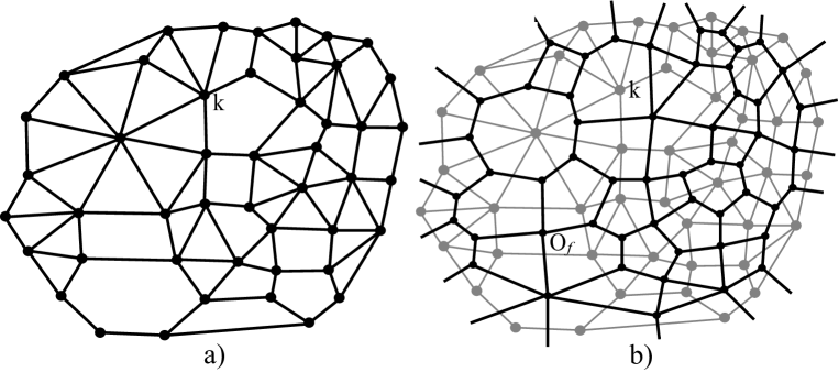
Figure 1. a) The cell complex $\mathcal{C}=(V,E,F)$ and b) its dual $\mathcal{C}^{*}=(V^{*},E^{*},F^{*})$

For the rest of this article, $V$ will be a finite set of points on $S$. Furthermore, by $\mathcal{C}=(V,E,F)$ we will denote a topological cell complex of $S$, where $V$ are the vertices, $E$ are the edges and $F$ are the faces of $\mathcal{C}$ (see figure 1a). All three sets are assumed to be finite. Furthermore, whenever a cone-metric $d$ is introduced on $S$, the condition $\text{sing}(d)\subseteq V$ always holds. In order to simplify notations, we will also assume that all cell complexes involved in this study have the following regularity properties.

$\bullet$ Any pair of edges from a cell complex either (i) coincide, (ii) have exactly one vertex in common or (iii) are disjoint with no vertices in common.

$\bullet$ Any pair of faces either (i) coincide, (ii) have exactly one vertex in common, (iii) have exactly one edge in common, or (iv) are disjoint with no vertices or edges in common.

This restriction is not essential and all results that follow will also apply to more general cell complexes. However, with this assumption in mind, the notations and the exposition become much lighter. Indeed, let $i,j\in V$ be two vertices that are endpoints of the same edge. Then, by assumption, $i$ and $j$ should be different and the notation $ij\in E$ uniquely determines the edge, because there cannot be another edge with both $i$ and $j$ as endpoints. Similarly, if $i_{1},...,i_{n}$ are all the vertices of a two-cell $f\in F$, then they are all different and the cell is uniquely determined by the notation $f=i_{1}...i_{n}\in F$.

Definition 2.1.

A geodesic cell complex on $(S,d)$ is a cell complex $\mathcal{C}_{d}=(V,E_{d},F_{d})$ whose edges, with endpoints removed, are geodesic arcs embedded in $S\setminus V$. Thus, each face from $F_{d}$ is isometric to a compact geodesic polygon in $\mathbb{F}^{2}$.

In other words, we can think of a geodesic cell-complex $\mathcal{C}_{d}$ on a geometric surface $(S,d)$ as a two dimensional manifold, obtained by gluing together geodesic polygons along their edges. The edges that we identify should have the same length and the identification should be an isometry. Notice the difference between a topological cell complex $\mathcal{C}$ and a geodesic cell complex $\mathcal{C}_{d}$. While $\mathcal{C}$ is just a purely topological (and hence combinatorial) object, the geodesic one $\mathcal{C}_{d}$ consists of polygons with geodesic edges and thus provides the underlying surface $S$ with a cone-metric $d$.

Assume three circles $c_{i},c_{j}$ and $c_{k}$ with centers $i,j$ and $k$ respectively, lie in the geometric plane $\mathbb{F}^{2}$. Moreover, let the circles’ interiors be disjoint. Then, there exists a unique forth circle $c_{\Delta}$ orthogonal to $c_{i},c_{j}$ and $c_{k}$. Furthermore, draw the geodesic triangle $\Delta=ijk$, spanned by the centers $i,j$ and $k$. Then $\Delta$, together with the circles $c_{i},c_{j},c_{k}$ and $c_{\Delta}$, is called a decorated triangle (see figure 2a). The circles $c_{i},c_{j}$ and $c_{k}$ are called the vertex circles of $\Delta$, while $c_{\Delta}$ is called the face circle of $\Delta$. We point out here that in this article it is allowed for one, two or all three vertex circles to degenerate to points. Even in this more general set up, everything said above still applies.

Remark. There is a slight subtlety in the case of $\mathbb{H}^{2}$. Although the vertex circles are always circles in the usual, natural sense, the face circle may fit a more general definition. For more details, see section 5.

Now, assume two non-overlapping decorated triangles, like $\Delta_{1}=jis$ and $\Delta_{2}=uis$ from figure 2a share a common edge $is$. As usual, denote by $c_{i},c_{j},c_{s}$ and $c_{u}$ the vertex circles (some of which may be shrunk to points), and by $c_{\Delta_{1}}$ and $c_{\Delta_{2}}$ the corresponding face circles of the triangles. Although, in general, the two face circles $c_{\Delta_{1}}$ and $c_{\Delta_{2}}$ are different, sometimes it may happen that they coincide, i.e. $c_{\Delta_{1}}=c_{\Delta_{2}}=c_{q}$. In that case all four vertex circles $c_{i},c_{j},c_{s}$ and $c_{u}$ are orthogonal to $c_{q}$. Thus, we can erase the edge $is$ and obtain a decorated geodesic quadrilateral $q=ijsu$ with vertex circles $c_{i},c_{j},c_{s}$ and $c_{u}$, and a face circle $c_{q}$. Observe, that in this case the quadrilateral is convex. If we continue this way, we can obtain various decorated polygons, like for instance the decorated pentagon $f^{\prime}=ijvsu$ from figure 2a.

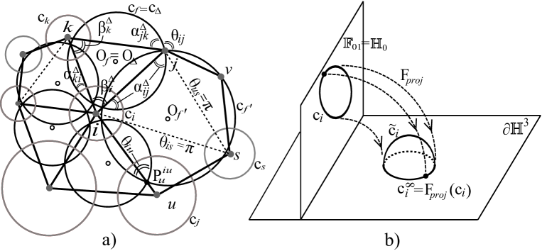
Figure 2. a) A hyper-ideal circle pattern of decorated triangles, polygons and labels; b) The projection $F_{proj}$ from the hyperbolic plane $\mathbb{H}_{0}\subset\mathbb{H}^{3}$ to the ideal boundary $\partial\mathbb{H}^{3}$.

Definition 2.2.

A decorated polygon is a convex geodesic polygon $p$ in $\mathbb{F}^{2}$, with vertices in labelled in cyclic order $i_{1},i_{2},...,i_{n}$, together with:

$\bullet$ a set of circles $c_{i_{1}},c_{i_{2}},...,c_{i_{n}}$ with disjoint interiors such that each $c_{i_{s}}$ is centered at vertex $i_{s}$ for $s=1,..,n$. Some or all of the circles are allowed to be points, i.e. circles of radius zero;

$\bullet$ another circle $c_{p}$ orthogonal to $c_{i_{1}},...,c_{i_{n}}$.

The circles $c_{i_{1}},...,c_{i_{n}}$ are called vertex circles and the additional orthogonal circle $c_{p}$ is called the face circle of the decorated polygon $p$.

Remark: Observe, that the vertex circles are assumed to have disjoint interiors. That means that all vertex circles could be either disjoint or some of them could be tangent to one another.

Whenever two faces of a cell complex share a common edge, we will say that the two faces are adjacent to each other. Furthermore, assume two decorated polygons $p_{1}$ and $p_{2}$ share a common geodesic edge $ij$, where $i$ and $j$ are the endpoints of $ij$, which also means that they are common vertices for both $p_{1}$ and $p_{2}$. Then, the decorated polygons $p_{1}$ and $p_{2}$ are called compatibly adjacent whenever the vertex circles $c_{i}^{1},c_{j}^{1}$ of $p_{1}$ and $c_{i}^{2},c_{j}^{2}$ of $p_{2}$ coincide respectively, that is $c_{i}^{1}\equiv c_{i}^{2}$ and $c_{j}^{1}\equiv c_{j}^{2}$. Furthermore, whenever two decorated polygons are compatibly adjacent, we will say that their face circles are adjacent to each other. A situation like that is depicted on figure 2a for the edge $ij$ and the two faces $f\equiv\Delta$ and $f^{\prime}$ with face circles $c_{f}$ and $c_{f^{\prime}}$.

Definition 2.3.

Let $p_{1}$ and $p_{2}$ be two decorated polygons in $\mathbb{F}^{2}$ that are compatibly adjacent to each other. Let $ij$ be their common geodesic edge. Furthermore, let $c_{p_{1}}$ and $c_{p_{2}}$ be the face circles of $p_{1}$ and $p_{2}$ respectively.

$\bullet$ We say that the edge $ij$ satisfies the local Delaunay property whenever each vertex circle of the decorated polygon $p_{2}$ is either (i) disjoint from the interior of the face circle $c_{p_{1}}$ of $p_{1}$, or (ii) if it is not, the intersection angle between the vertex circle in question and the face circle $c_{p_{1}}$ is less than $\pi/2$. See for instance edge $ij$ on figure 2a.

$\bullet$ For the edge $ij$, which satisfies the local Delaunay property, $\theta_{ij}\in[0,\pi)$ denotes the intersection angle between the two adjacent face circles $c_{p_{1}}$ and $c_{p_{2}}$, measured between the circular arcs that bound the region of common intersection. (See for example angles $\theta_{ij},\theta_{iu},\theta_{is}$ and $\theta_{us}$ from figure 2a.)

It is not difficult to see that the definition of a local Delaunay property is symmetric in the sense that if the condition of definition 2.3 holds for the face circle $c_{p_{1}}$ and the vertex circles of $p_{2}$, then it also holds for the face circle $c_{p_{2}}$ and the vertex circles of $p_{1}$.

Definition 2.4.

A hyper-ideal circle pattern on a given surface $S$ (figure 2a) is a hyperbolic or Euclidean cone-metric $d$ on $S$ together with a geodesic cell complex $\mathcal{C}_{d}=(V,E_{d},F_{d})$ whose faces are decorated geodesic polygons such that any two adjacent faces are compatibly-adjacent and each geodesic edge of $\mathcal{C}_{d}$ has the local Delaunay property. Whenever $d$ is flat on $S\setminus V$, we call the circle pattern Euclidean, and whenever $d$ is hyperbolic on $S\setminus V$, we call the pattern hyperbolic.

Intuitively speaking, a hyper-ideal circle pattern on a surface $S$ is a surface homeomorphic to $S$, obtained by gluing together decorated geodesic polygons along pairs of corresponding edges. The edges that are being identified should have the same length, the identification should be an isometry and the vertices that get identified should have vertex-circles with same radii.

Observe that a hyper-ideal circle pattern on $S$ consists of (i) a cone-metric $d$ on $S$, (ii) a set of vertices $V\supseteq\text{sing}(d)$, (iii) an assignment of vertex radii $r$ on $V$, and (iv) a geodesic cell complex $\mathcal{C}_{d}$ together with (v) a collection of vertex circles and (vi) a collection of face circles. However, the geometric data $(S,d,V,r)$ is enough to further identify uniquely the geodesic cell complex $\mathcal{C}_{d}$ and the collections of vertex and face circles. This is done via the weighted Delaunay cell decomposition construction. More precisely, given (i) a geometric surface $(S,d)$, (ii) a finite set of points $V\supset\text{sing}(d)$ on $S$ and (iii) an assignment of disjoint vertex circle radii $r:V\to[0,\infty)$, one can uniquely generate (obtain) the corresponding $r-$weighted Delaunay cell complex $\mathcal{C}_{d}$, where each edge satisfies the local Delaunay property. In the process, the families of vertex and face circles naturally appear as part of the construction [6, 21, 19]. Alternatively, one can obtain the $r-$weighted Delaunay cell decomposition as the geodesic dual to the $r$-weighted Voronoi diagram, also known as the weighted power diagram with weights $r$ [6]. A Voronoi cell in the case when $d$ is Euclidean is defined as $W_{d,r}(i)=\big{\{}x\in S\,|\,d(x,i)^{2}-r_{i}^{2}\leq d(x,j)^{2}-r_{j}^{2}\,\,\text{for all}\,\,j\in V\,\big{\}}$. A Voronoi cell in the case when $d$ is hyperbolic is defined as $W_{d,r}(i)=\big{\{}x\in S\,|\,\cosh{(r_{j})}\cosh{d(x,i)}\leq\cosh{(r_{i})}\cosh{d(x,j)}\,\,\text{for all}\,\,j\in V\,\big{\}}$.

3. The circle pattern problem and the main result

Let us fix an arbitrary hyper-ideal circle pattern on $S$ and let this pattern be determined by the data $(S,d,V,r)$. Figure 2a depicts (a portion of) a hyper-ideal circle pattern. For each vertex $i\in V$ one can define $\Theta_{i}>0$ to be the cone angle of the cone-metric $d$ at vertex $i$. Furthermore, since $S$ is a closed surface, each edge $ij\in E_{d}$ is the common edge of exactly two faces from the $r$-weighted Delaunay cell-complex $\mathcal{C}_{d}=(V,E_{d},F_{d})$. Call these faces $f$ and $f^{\prime}\in F_{d}$, one on each side of the edge. Consequently, one can associate to each edge $ij$ the pair of adjacent face circles $c_{f}$ and $c_{f^{\prime}}$. As a result of this, one can assign to $ij$ the intersection angle $\theta_{ij}\in[0,\pi)$ between $c_{f}$ and $c_{f^{\prime}}$, as explained in definition 2.3 and shown on figure 2a.

Observe that given any hyper-ideal circle pattern on $S$, like the one from the preceding paragraph, one can always extract from it the combinatorial data $(\mathcal{C},\theta,\Theta)$, where $\mathcal{C}$ is the $r-$weighted Delaunay cell decomposition $\mathcal{C}_{d}$ viewed as a purely topological complex, $\Theta:V\to(0,\infty)$ is the assignment of cone angles at the vertices of the complex and $\theta:E_{d}\to[0,\pi)$ is the assignment of intersection angles between adjacent face circles of the pattern. In this case, we will say that the given hyper-ideal circle pattern realizes the (combinatorial angle) data $(\mathcal{C},\theta,\Theta)$.

The central scope of the current article is to answer the question whether the procedure described in the previous paragraph can be reversed. Compare with [19].

Circle Pattern Problem.

Assume the combinatorial data $(\mathcal{C},\theta,\Theta)$ is provided, where

• $\mathcal{C}=(V,E,F)$ is a topological cell complex on a surface $S$;

• $\theta:E\to[0,\pi)\,\,\,\,\text{ and }\,\,\,\,\Theta:V\to(0,\infty)$.

Find a hyperbolic or flat cone metric $d$ on $S$, together with a hyper-ideal circle pattern on it that realizes the data $(\mathcal{C},\theta,\Theta)$.

In this article, we provide a solution to the circle pattern problem in the following form (see also [19]).

Theorem 1.

Let $S$ be a closed surface with a topological cell complex $\mathcal{C}=(V,E,F)$ on it. There exist two convex polytopes $\mathcal{P}_{S,\mathcal{C}}^{h}$ and $\mathcal{P}_{S,\mathcal{C}}^{e}$, depending on the combinatorics of $\mathcal{C}$ and containing points of type $(\theta,\Theta)\in\mathbb{R}^{E}\times\mathbb{R}^{V}$, for which the following statements hold:

E. The combinatorial data $(\mathcal{C},\theta,\Theta)$ is realized by a Euclidean hyper-ideal circle pattern on $S$ if and only if $(\theta,\Theta)\in\mathcal{P}_{S,\mathcal{C}}^{e}$. Furthermore, this pattern is unique up to scaling and isometry between hyperbolic cone-metrics on $S$, isotopic to identity.

H. The combinatorial data $(\mathcal{C},\theta,\Theta)$ is realized by a hyperbolic hyper-ideal circle pattern on $S$ if and only if $(\theta,\Theta)\in\mathcal{P}_{S,\mathcal{C}}^{h}$. Furthermore, this pattern is unique up to isometry between hyperbolic cone-metrics on $S$, isotopic to identity.

In both cases, whenever the hyper-ideal circle pattern exists, it can be reconstructed from the unique critical point of a strictly convex functional defined on a suitably chosen open subset of $\mathbb{R}^{N}$ for some $N\in\mathbb{N}$.

Remark: The two polytopes $\mathcal{P}_{S,\mathcal{C}}^{h}$ and $\mathcal{P}_{S,\mathcal{C}}^{e}$ are called angle data polytopes. Their explicit definition is given in the next section. For both of them we will use the common notation $\mathcal{P}_{S,\mathcal{C}}$.

4. Description of the angle data polytopes

In this section we give an explicit description of the two polytopes $\mathcal{P}_{S,\mathcal{C}}^{h}$ and $\mathcal{P}_{S,\mathcal{C}}^{e}$ from theorem 1.

Assume a cell complex $\mathcal{C}=(V,E,F)$ is fixed on the surface $S$ (see figure 1a). Denote by $\mathcal{C}^{*}=(V^{*},E^{*},F^{*})$ the cell complex dual to $\mathcal{C}$, where $V^{*}$ are the dual vertices, $E^{*}$ are the dual edges and $F^{*}$ are the dual faces (see figure 1b). The dual vertices are in bijective correspondence with the faces of $\mathcal{C}$. To simplify things, we can assume that each face $f\in F$ contains exactly one vertex $O_{f}\in V^{*}$ in its interior. The dual edges are obtained as follows: if $f$ and $f^{\prime}\in F$ are two adjacent faces of $\mathcal{C}$ and $ij\in E$ is their common edge, then there exists a dual edge $ij^{*}=O_{f}O_{f^{\prime}}\in E^{*}$ which connects the dual vertices $O_{f}$ and $O_{f^{\prime}}\in V^{*}$. Just like with the dual vertices, the dual faces are in bijective correspondence with the vertices of $\mathcal{C}$ and again we can assume that the former contain the latter in their interiors. On figure 1b the elements of the original complex $\mathcal{C}$ are drawn in grey, while the elements of the dual complex $\mathcal{C}^{*}$ are in black.

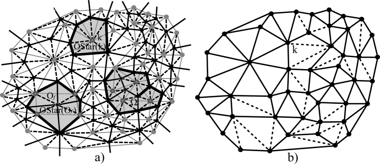
Figure 3. a) The triangulation $\hat{\mathcal{T}}=(\hat{V},\hat{E},\hat{F})$ together with two examples of open stars and one admissible domain $\Omega$; b) The subtriangulation $\mathcal{T}=(V,E_{T},F_{T})$ of $\mathcal{C}$ whose dashed edges are the auxiliary edges from $E_{\pi}$.

Next, define the subdivision $\hat{\mathcal{T}}=(\hat{V},\hat{E},\hat{F})$ of $\mathcal{C}^{*}$, depicted on figure 3a, where

$\bullet$ $\hat{V}=V\cup V^{*}$, i.e. the vertices of $\hat{\mathcal{T}}$ consist of all vertices of $\mathcal{C}$ and all dual vertices. These are all black and grey vertices from figures 1b and 3a;

$\bullet$ $\hat{E}=E^{*}\cup\big{\{}\,iO_{f}\,\,|\,\,O_{f}\in V^{*}\,\,\text{and $i$ is a vertex of $f$ }\big{\}}$, i.e. the edges of $\hat{\mathcal{T}}$ consist of all dual edges and all edges, obtained by connecting a dual vertex $O_{f}\in f$ to all the vertices of the face $f\in F$ it belongs to. The latter type of edges will be called corner edges. The dual edges can be seen on both figures 1b and 3a painted solid black, while the corner edges are the black dashed edges from figure 3a.

$\bullet$ $\hat{F}=\bigl{\{}iO_{f}O_{f^{\prime}}\,|\,\text{ $ij\in E$ common edge for $f$ and $f^{\prime}$ from $F$ }\bigr{\}},$ i.e. the faces of $\hat{\mathcal{T}}$ are the topological triangles obtained by looking at the connected components of the complement of the topological graph $(\hat{V},\hat{E})$ on $S$. On figure 3a these are the triangles with one solid black and two dashed black edges. They also have two black (dual) vertices and one grey vertex.

The next important notion to be defined is, what we call in this paper, the open star of a vertex from $\hat{\mathcal{T}}$.

Definition 4.1.

Let $\hat{v}\in\hat{V}$ be an arbitrary vertex of $\hat{\mathcal{T}}.$ Then its open star $\text{\emph{OStar}}(\hat{v})$ is defined as the open interior of the union of all closed triangles from $\hat{\mathcal{T}}$ which contain $\hat{v}$.

In particular, whenever $\hat{v}=k\in V$ is a vertex of $\mathcal{C}$, then its open star is simply the open interior of the face from $\mathcal{C}^{*}$ dual to $k$. An example denoted by $\text{OStar}(k)$ and colored in grey is shown on figure 3a. Then, as one can see, the boundary of $\text{OStar}(k)$ consists entirely of dual edges from $E^{*}$. If we denote by $E_{k}$ the set of all edges of $\mathcal{C}$ which have vertex $k$ as an endpoint, then $\partial\,\text{OStar}(k)=\cup\bigl{\{}ik^{*}\in E^{*}\,\,|\,\,ik\in E_{k}\,\bigr{\}}$. If $\hat{v}=O_{f}\in V^{*}$ is a vertex from the dual complex $\mathcal{C}^{*}$, then the boundary of its open star consists entirely of corner edges from $\hat{\mathcal{T}}$ (see the grey region $\text{OStar}(O_{f})$ on figure 3a).

Before we continue, let us go back to the original cell complex $\mathcal{C}=(V,E,F)$. We are going to partition the set of its vertices and edges depending on where we want the circle pattern realizations of $\mathcal{C}$ to have vertex circles of radius zero and edges with tangent vertex circles centered at their endpoints. Let

$\bullet$ $V=V_{0}\cup V_{1}$, where $V_{0}\cap V_{1}=\varnothing$;

$\bullet$ $E=E_{0}\cup E_{1}$, where $E_{0}\cap E_{1}=\varnothing$ and for any $ij\in E_{0}$ both $i$ and $j$ belong to $V_{1}$.

Following the terminology of [19], one can define what Schlenker calls an admissible domain. Our definition however is more restrictive than his in the sense that we select a much smaller collection of admissible domains than the ones described in [19]. Thus we have decreased the number of conditions on the angle data that appear in theorem 2 below.

Definition 4.2.

An open connected subdomain $\Omega$ of the surfaces $S$ is called an admissible domain of $(S,\mathcal{C})$ whenever the following conditions hold:

1. There exists a subset $\hat{V}_{0}\subseteq\hat{V}$, such that $\Omega=\cup\big{\{}\text{\emph{OStar}}(\hat{v})\,\,|\,\,\hat{v}\in\hat{V}_{0}\big{\}};$

2. $\Omega\neq\varnothing$ and $\Omega\neq S$ and $\Omega\cap V\neq\varnothing$;

A special example of an admissible domain is the open star of a vertex of $\mathcal{C}$. The open star of a dual vertex however is not an admissible domain because it is disjoint from $V$. An example of an admissible domain can be seen on figure 3a, denoted by the symbol $\Omega$ and shaded in grey. On this picture $\Omega$ is simply connected but in general it doesn’t have to be.

The boundary of an admissible domain $\Omega$ is a disjoint union of immersed in $S$ topologically polygonal curves, consisting entirely of edges from the triangulation $\hat{\mathcal{T}}$. In other words, the boundary of $\Omega$ consists of dual edges and/or corner edges from $\hat{E}$, but all of its connected components are interpreted as immersed closed paths in the one-skeleton of $\hat{\mathcal{T}}$, so that some of the edges could be traced (counted) twice (see figure 3a). That happens exactly when an edge of $\hat{\mathcal{T}}$ is disjoint from $\Omega$, but the interiors of the two topological triangles from $\hat{\mathcal{T}}$, lying on both sides of the edge, are contained in $\Omega$. We denote this immersed version of the boundary of $\Omega$ by $\partial\Omega$.

Theorem 2.

In the setting of theorem 1, the polytopes $\mathcal{P}_{S,\mathcal{C}}^{h}$ and $\mathcal{P}_{S,\mathcal{C}}^{e}$ are defined as follows (compare to [19]):

E. Euclidean case. A point $(\theta,\Theta)\in\mathbb{R}^{E_{1}}\times\mathbb{R}^{V_{1}}$ belongs to $\mathcal{P}_{S,\mathcal{C}}^{e}$ exactly when:

E1) For any $ij\in E_{0}$ let $\theta_{ij}=0$ while $\theta_{ij}\in(0,\pi)$ for $ij\in E_{1}$;

E2) For any $k\in V_{0}$ let $\Theta_{k}=\sum_{ik\in E_{k}}(\pi-\theta_{ik})$. This is equivalent to $\Theta_{k}=\sum_{ik^{*}\subset\partial\Omega}(\pi-\theta_{ik})$ for $\Omega=\text{\emph{OStar}}(k)$. Also $\Theta_{k}>0$ for all $k\in V_{1}$;

E3) $\sum_{k\in V}(2\pi-\Theta_{k})=2\pi\chi(S)$;

E4) For any admissible domain $\Omega$ of $(S,\mathcal{C})$, such that $\Omega\neq\text{\emph{OStar}}(k)$ for some $k\in V_{0}$,

$$\sum_{ij^{*}\subset\partial\Omega}(\pi-\theta_{ij})+\sum_{k\in\Omega\cap V}(2\pi-\Theta_{k})>2\pi\chi(\Omega)-\pi|\partial\Omega\cap V|.$$ (1)

H. Hyperbolic case. A point $(\theta,\Theta)\in\mathbb{R}^{E_{1}}\times\mathbb{R}^{V_{1}}$ belongs to $\mathcal{P}_{S,\mathcal{C}}^{h}$ exactly when:

H1) For any $ij\in E_{0}$ let $\theta_{ij}=0$ while $\theta_{ij}\in(0,\pi)$ for $ij\in E_{1}$;

H2) For any $k\in V_{0}$ let $\Theta_{k}=\sum_{ik\in E_{k}}(\pi-\theta_{ik})$. Put in another way, $\Theta_{k}=\sum_{ik^{*}\subset\partial\Omega}(\pi-\theta_{ik})$ for $\Omega=\text{\emph{OStar}}(k)$. Also $\Theta_{k}>0$ for all $k\in V_{1}$;

H3) $\sum_{k\in V}(2\pi-\Theta_{k})>2\pi\chi(S)$;

H4) For any admissible domain $\Omega$ of $(S,\mathcal{C})$, such that $\Omega\neq\text{\emph{OStar}}(k)$ for some $k\in V_{0}$,

$$\sum_{ij^{*}\subset\partial\Omega}(\pi-\theta_{ij})+\sum_{k\in\Omega\cap V}(2\pi-\Theta_{k})>2\pi\chi(\Omega)-\pi|\partial\Omega\cap V|.$$

Here $\chi(S)$ and $\chi(\Omega)$ are the Euler characteristics of $S$ and $\Omega$ respectively.

Condition (1) can be also written as

$$\sum_{ij^{*}\subset\partial\Omega\cap E_{1}}(\pi-\theta_{ij})+\sum_{k\in\Omega\cap V}(2\pi-\Theta_{k})>2\pi\chi(\Omega)-\pi|\partial\Omega\cap V|-\pi|\partial\Omega\cap E_{0}|.$$

We are going to assume that the vector space $\mathbb{R}^{E_{1}}\times\mathbb{R}^{V_{1}}$ is an affine subspace of $\mathbb{R}^{E}\times\mathbb{R}^{V}$ by assuming that any $(\theta,\Theta)\in\mathbb{R}^{E_{1}}\times\mathbb{R}^{V_{1}}$ is extended to a point in $\mathbb{R}^{E}\times\mathbb{R}^{V}$ by letting $\theta_{ij}=0$ for all $ij\in E\setminus E_{1}=E_{0}$, and $\Theta_{k}=\sum_{ik\in E_{k}}(\pi-\theta_{ik})$ for all $k\in V\setminus V_{1}=V_{0}$. Thus, one can naturally assume that the polytopes $\mathcal{P}_{S,\mathcal{C}}^{h}$ and $\mathcal{P}_{S,\mathcal{C}}^{e}$ are in the larger space $\mathbb{R}^{E}\times\mathbb{R}^{V}$.

To optimize the conditions from theorem 2 a bit more, one can define the so called strict admissible domain.

Definition 4.3.

An open connected subdomain $\Omega$ of the surfaces $S$ is called a strict admissible domain of $(S,\mathcal{C})$ whenever $\Omega$ is admissible and $\partial\Omega\cap V_{0}=\varnothing$.

As it turns out, the angle data polytopes can be described via strict admissible domains instead of admissible domains. In fact, the admissible domains which are not strict do not add more restrictions to the angle data, i.e. they produce redundant conditions.

Corollary 4.1.

The statements of theorem 2 still hold even if the expression “admissible domain” in points E4 and H4 of theorem 2 is replaced by the expression “strict admissible domain”.

5. Some basic geometric facts

In what follows, we state some basic facts from Euclidean and hyperbolic geometry, which will be useful in our investigation.

The primary models of the hyperbolic plane $\mathbb{H}^{2}$, used in this article, are the two standard conformal models - the upper half-plane and the Poincaré disc. The term “conformal” means that in both of these models, the measure of angle with respect to the hyperbolic metric equals the measure of angle with respect to the underlying Euclidean metric. Although the notion of a circle in Euclidean geometry is well-known, circles in the hyperbolic plane require some attention. Let a regular circle in $\mathbb{H}^{2}$ be defined as a curve in $\mathbb{H}^{2}$ consisting of all points which are equidistant from a given point, called the center of the circle. In addition to that, let a hyper-circle in $\mathbb{H}^{2}$ be defined as a curve in $\mathbb{H}^{2}$, equidistant from a given geodesic, called the central geodesic, and lying on one side of that geodesic. Then the word circle in $\mathbb{H}^{2}$ (or alternatively hyperbolic circle) is the common term we use for regular circles, horocycles (see [22, 23, 9] or [5]) and hyper-circles. Furthermore, regular circles and horocycles have well defined interiors, i.e. they have discs. Consequently, a regular circle is the boundary curve of a regular disc and a horocycle is the boundary curve of a horodisc. Analogously, a hyper-disc is a connected subdomain of $\mathbb{H}^{2}$, whose boundary curve is a hyper-circle with a central geodesic contained in the hyper-disc. Consequently, the word disc in $\mathbb{H}^{2}$ (or alternatively hyperbolic disc) is the common term for regular discs, horodiscs and hyper-discs. Thus, inside a circle means inside the disc of the circle in question.

A very useful property of the Poincaré disc and the upper-half plane is that hyperbolic circles are exactly the intersections of the model with ordinary Euclidean circles (circles in the underlying Euclidean geometry). In this line of thoughts, a regular circle in $\mathbb{H}^{2}$ is in fact a Euclidean circle fully contained in $\mathbb{H}^{2}$. The only peculiarity here is that, generically speaking, the hyperbolic center of a regular circle in $\mathbb{H}^{2}$ is different from its Euclidean center. Furthermore, a hyper-circle in $\mathbb{H}^{2}$ is the circular arc obtained from the intersection of a Euclidean circle with $\mathbb{H}^{2}$, where the Euclidean circle intersects $\partial\mathbb{H}^{2}$ at exactly two points. The geodesic between these two ideal points is the central geodesic of the hyper-circle. In particular, hyperbolic geodesics are a special type of hyper-circles, orthogonal to $\partial\mathbb{H}^{2}$, i.e. we can think that their “hyperbolic radius” is equal to zero. Finally, a horocycle is in general a Euclidean circle inside $\mathbb{H}^{2}$ tangent to $\partial\mathbb{H}^{2}$.

Since circle patterns are traditionally linked to polyhedral objects in the hyperbolic three-space $\mathbb{H}^{3}$, a fact which we will exploit a lot in this article, we will strongly rely on the upper half-space model of $\mathbb{H}^{3}$. Just like in the case of $\mathbb{H}^{2}$ the latter is a conformal model and shares analogous properties with the upper-half plane.

It is worth mentioning that the disc can be transformed into the upper-half plane by a planar Möbius transformation. Here is one way to do this. For notational simplicity, identify the plane with $\mathbb{C}$. Let $\mathbb{H}^{2}_{up}$ be the upper-half plane $\{\text{Im}(z)>0\}$ and $\mathbb{H}^{2}_{d}$ be the unit disc $\{|z|<1\}$. Furthermore, draw circle $c_{0}$ centered at $-i=-\sqrt{-1}$ and passing through the points $-1$ and $1$. Then it is immediate to see that the inversion in $c_{0}$ maps $\mathbb{H}^{2}_{d}$ to $\mathbb{H}^{2}_{up}$. Consequently, one can easily carry constructions from the unit disc to the upper-half plane and vice versa. From now on by $l_{\mathbb{H}^{2}}(MN)$ and $l_{\mathbb{H}^{3}}(MN)$ we denote the hyperbolic length of a geodesic segment $MN$, and by $|MN|$ we denote the length of the straight-line segment $MN$ with respect to the background Euclidean geometry. Also, we would denote by $l_{\mathbb{F}^{2}}(MN)$ the distance between $M$ and $N$ in the plane $\mathbb{F}^{2}$. For more details on two and three dimensional hyperbolic geometry, one can consult for example [22, 23, 9] or [5].

Remark. In this section, we have chosen to present proofs based on compass and straightedge constructions with the presumption that these may turn out useful for certain applications, such as computer realizations for instance.

Proposition 5.1.

Let circles $c_{f}$ and $c_{f^{\prime}}$ in $\mathbb{F}^{2}$ intersect in exactly two points $P_{i}^{ij}$ and $P_{j}^{ij}$. Let $Ra_{ij}$ be the geodesic passing through both points $P_{i}^{ij}$ and $P_{j}^{ij}$. Furthermore, denote by $\tilde{R}a_{ij}$ the geodesic $Ra_{ij}$ with the closed geodesic segment $P_{i}^{ij}P_{j}^{ij}$ removed from it. Then

1. Any point form $\tilde{R}a_{ij}$ is the center of exactly one circle orthogonal to both $c_{f}$ and $c_{f^{\prime}}$;

2. If the point $O$ from $\tilde{R}a_{ij}$, is the center of a circle $c$ orthogonal to $c_{f}$, then $c$ is also orthogonal to $c_{f^{\prime}}$;

3. If a circle $c$ is orthogonal to both circles $c_{f}$ and $c_{f^{\prime}}$, then its center $O$ lies on $\tilde{R}a_{ij}$. In the case of $\mathbb{F}^{2}=\mathbb{H}^{2}$, the circle $c$ is assumed to be regular.

Proof.

Euclidean case. When $\mathbb{F}^{2}$ is the Euclidean plane, the statement of this proposition follows from the properties of the radical axis of a pair of intersecting circles.

Hyperbolic case. The hyperbolic case follows from the Euclidean case, combined with some basic properties of the Poincaré disc model. Denote by $O_{\mathbb{H}^{2}}$ the Euclidean center of the Poincaré disc $\mathbb{H}^{2}$. Whenever the hyperbolic center $O$ of a circle $c$ in $\mathbb{H}^{2}$ coincides with $O_{\mathbb{H}^{2}}$ then $O\equiv O_{\mathbb{H}^{2}}$ is also the Euclidean center of $c$. Thus, in order to complete the proof of the current proposition, it is enough to move the point $O$, via a hyperbolic isometry of $\mathbb{H}^{2}$, to $O_{\mathbb{H}^{2}}$. Then one can apply the Euclidean case. After that, one can use the fact that the straight line $Ra_{ij}$ passes through $O_{\mathbb{H}^{2}}$ and consequently its intersection with $\mathbb{H}^{2}$ is a hyperbolic geodesic. ∎

Corollary 5.1.

Let $f$ and $f^{\prime}$ be two compatibly adjacent decorated polygons in $\mathbb{F}^{2}$, sharing a common edge $ij$. Let their corresponding face circles be $c_{f}$ and $c_{f^{\prime}}$. Then the two points of intersection $P^{ij}_{i}$ and $P^{ij}_{j}$ of $c_{f}$ and $c_{f^{\prime}}$ lie on the common edge $ij$.

This last corollary allows us to define the intersection angle between the face circles of two adjacent decorated polygons.

Definition 5.1.

Let two compatibly adjacent decorated polygons $f$ and $f^{\prime}$ share a common edge $ij$ and have corresponding face circles $c_{f}$ and $c_{f^{\prime}}$. In accordance with corollary 5.1, let $P^{ij}_{i}$ and $P^{ij}_{j}$ be the two intersection points of the circles $c_{f},c_{f^{\prime}}$ and the edge $ij$. Point $P^{ij}_{i}\in ij$ is the closer one to vertex $i$, while $P^{ij}_{j}\in ij$ is the closer on to vertex $j$. The points $P^{ij}_{i}$ and $P^{ij}_{j}\in c_{f}$ split the circle $c_{f}$ into two circular arcs. Denote by $c_{f}(ij)\subset c_{f}$ the arc whose interior is disjoint from the edges of $f$. In the same way, define the arc $c_{f^{\prime}}(ij)\subset c_{f^{\prime}}$. Then, the intersection angle $\theta_{ij}\in[0,2\pi)$ between $c_{f}$ and $c_{f^{\prime}}$ is defined to be the angle between the arcs $c_{f}(ij)$ and $c_{f^{\prime}}(ij)$ measured inside the bounded region the two arcs enclose (see figure 2a).

A straightforward consequence of definition 5.1 is the following statement

Proposition 5.2.

In the setting of definition 5.1, the angle $\theta_{ij}=0$ if and only if the face circles $c_{f}$ and $c_{f^{\prime}}$ are tangent to the edge $ij$ and to each other at the point $P^{ij}_{i}\equiv P^{ij}_{j}$. Furthermore, $\theta_{ij}=\pi$ if and only if the two face circles coincide, i.e. $c_{f}\equiv c_{f^{\prime}}$. (See for example edges $is$ and $js$ on figure 2a.)

A ray in $\mathbb{F}^{2}$ is a geodesic half-line. In other words, this is a Euclidean half-line, in the case of $\mathbb{E}^{2}$, and a hyperbolic half-geodesic, in the case of $\mathbb{H}^{2}$. We denote a ray by $A\overrightarrow{r}$, where $A$ is the ray’s point of origin. If a ray starts from a point $A$ and passes through a point $B$, then it can be also denoted by $\overrightarrow{AB}$. Let $A\overrightarrow{r_{1}}$ and $A\overrightarrow{r_{2}}$ be two rays with a common origin $A$. Denote by $\alpha_{0}=\measuredangle r_{1}Ar_{2}$ the angle between them, fixed so that $\alpha_{0}\in(0,\pi)$. Then $Dom_{12}$ is chosen to be the closed convex domain bounded by the two rays (infinite sector). Observe that the angle $\alpha_{0}$ is measured inside $Dom_{12}$. Let $c$ be a circle which intersects both $A\overrightarrow{r_{1}}$ and $A\overrightarrow{r_{2}}$. The angle between $c$ and $A\overrightarrow{r_{j}}$ is the angle $\alpha_{j}$ measured inside $Dom_{12}$ and outside $c$, or equivalently, measured inside $c$ and outside $Dom_{12}$. Finally, a homothety (uniform scaling) is a special similarity transformation of the Euclidean plane $\mathbb{E}^{2}$ which fixes a single point, called the center of the homothety, and maps each line through that point onto itself. In fact, the group of similarities of $\mathbb{E}^{2}$ is generated by all Euclidean isometries and homotheties. The latter preserve angles but not lengths. However, they preserve ratios of lengths.

Lemma 5.1.

Let $A$ be an arbitrary point in $\mathbb{F}^{2}$, and let $A\overrightarrow{r_{1}}$ and $A\overrightarrow{r_{2}}$ be two rays with common origin $A$. Let $\alpha_{0}\in(0,\pi)$ be the angle between the rays and let $\alpha_{1},\alpha_{2}\in(0,\pi)$ be such that $\alpha_{0}+\alpha_{1}+\alpha_{2}<\pi$. Then there is a unique ruler and compass constructible pair of rays $A\overrightarrow{t_{1}}$ and $A\overrightarrow{t_{2}}$ with a common origin $A$ that have the following properties:

1. A circle is tangent to both rays $A\overrightarrow{t_{1}}$ and $A\overrightarrow{t_{2}}$ if and only if its intersection angles with $A\overrightarrow{r_{1}}$ and $A\overrightarrow{r_{2}}$ are $\alpha_{1}$ and $\alpha_{2}$ respectively. When $\mathbb{F}^{2}=\mathbb{H}^{2}$, the circle is allowed to be a geodesic.

2. If a circle is tangent to $A\overrightarrow{t_{1}}$ and has intersection angle $\alpha_{1}$ with $A\overrightarrow{r_{1}}$, then it is tangent to $A\overrightarrow{t_{2}}$ and its intersection angle with $A\overrightarrow{r_{2}}$ is necessarily $\alpha_{2}$.

Proof.

Euclidean case. The proof of the Euclidean case will help us prove the hyperbolic version. We are aware of several ways one could go about the construction of the rays $A\overrightarrow{t_{1}}$ and $A\overrightarrow{t_{2}}$. However, we present just one of them.

1. Fix an arbitrary number $R>0$. Construct two isosceles triangles $\triangle X_{1}Y_{1}Z_{1}$ and $\triangle X_{2}Y_{2}Z_{2}$ such that (i) points $X_{j}$ and $Y_{j}$ lie on $A\overrightarrow{r_{j}}$, (ii) $|X_{j}Z_{j}|=|Y_{j}Z_{j}|=R$, (iii) $\measuredangle X_{j}Z_{j}Y_{j}=2\alpha_{j}$ and (iv) either point $Z_{j}\in Dom_{12}$, when $\alpha_{j}\in(0,\pi/2]$, or $Z_{j}$ and $Dom_{12}$ are separated by the line $X_{j}Y_{j}$, when $\alpha_{j}\in(\pi/2,\pi)$ (here $j\neq k=1,2$). Notice that at most one $\alpha_{j}$ can be greater or equal to $\pi/2$. Draw lines $l_{1}$ and $l_{2}$ such that $l_{1}$ passes through $Z_{1}$ and is parallel to $A\overrightarrow{r_{1}}$, while $l_{2}$ passes through $Z_{2}$ and is parallel to $A\overrightarrow{r_{2}}$. Let $O_{12}$ be the intersection point of $l_{1}$ and $l_{2}$. Draw a circle $c_{12}$ of radius $R$ with center $O_{12}$. The inequality $\alpha_{0}+\alpha_{1}+\alpha+2<\pi$ is equivalent to the fact that $A$ is outside $c_{12}$ which, in its own turn, is equivalent to the fact that $c_{12}$ intersects each ray $A\overrightarrow{r_{j}}$ at exactly two points, $j=1,2$. Then one can easily check that the intersection angles of the circle $c_{12}$ with the rays $A\overrightarrow{r_{1}}$ and $A\overrightarrow{r_{2}}$ are $\alpha_{1}$ and $\alpha_{2}$ respectively. Denote by $A\overrightarrow{r_{12}}$ the ray $\overrightarrow{AO_{12}}$. Furthermore, construct $A\overrightarrow{t_{1}}$ and $A\overrightarrow{t_{2}}$ as the two rays with a common point of origin $A$ and tangent to circle $c_{12}$. The indices $j=1,2$ are chosen so that the ray $A\overrightarrow{r_{1}}$ is the one between rays $A\overrightarrow{t_{1}}$ and $A\overrightarrow{r_{2}}$. Observe that $A\overrightarrow{r_{12}}$ bisects the angle $\measuredangle t_{1}At_{2}=\gamma_{0}\in(0,\pi)$, formed by the tangent rays $A\overrightarrow{t_{1}}$ and $A\overrightarrow{t_{2}}$.

Now let $c$ be any circle tangent to both $A\overrightarrow{t_{1}}$ and $A\overrightarrow{t_{2}}$. Then its center $O$ necessarily lies on the angle bisector $A\overrightarrow{r_{12}}$. Apply to $c_{12}$ the unique homothety with center $A$ which sends point $O_{12}$ to point $O$. Since this homothety maps the three rays $A\overrightarrow{t_{1}},A\overrightarrow{t_{2}}$ and $A\overrightarrow{r_{12}}$ to themselves, the image of the circle $c_{12}$ is again a circle, centered at $O\in A\overrightarrow{r_{12}}$ and tangent to both $A\overrightarrow{t_{1}}$ and $A\overrightarrow{t_{2}}$. But the circle $c$ is the unique circle centered at $O$ and tangent to $A\overrightarrow{t_{1}}$ (and consequently tangent to $A\overrightarrow{t_{2}}$ sa well). Hence $c$ is the image of $c_{12}$. By observing that the homothety also maps the rays $A\overrightarrow{t_{1}}$ and $A\overrightarrow{r_{2}}$ to themselves, as well as it preserves angles, we conclude that the intersection angles of $c$ with $A\overrightarrow{t_{1}}$ and $A\overrightarrow{r_{2}}$ equal the intersection angles of its preimage $c_{12}$ with $A\overrightarrow{t_{1}}$ and $A\overrightarrow{r_{2}}$, which by construction are $\alpha_{1}$ and $\alpha_{2}$ respectively.

Conversely, let a circle $c$, with a center $O$, intersect both rays $A\overrightarrow{r_{1}}$ and $A\overrightarrow{r_{2}}$ at angles $\alpha_{1}$ and $\alpha_{2}$ respectively. For $j=1,2$ let $Q_{j}$ be the farthest from $A$ intersection point of $c$ and $A\overrightarrow{r_{j}}$. Similarly, let $Q^{12}_{j}$ be the farthest from $A$ intersection point of the ray $A\overrightarrow{r_{j}}$ and the circle $c_{12}$ constructed above. Recall, $O_{12}\in A\overrightarrow{r_{12}}$ is the center of $c_{12}$. Since $\measuredangle OQ_{j}A=\pi/2-\alpha_{j}=\measuredangle O_{12}Q^{12}_{j}A$, the lines $OQ_{j}$ and $O_{12}Q^{12}_{j}$ are parallel. Let points $A_{1}$ and $A_{2}$ be the intersection points of the line $O_{12}O$ with the lines $Q^{12}_{1}Q_{1}$ and $Q^{12}_{2}Q_{2}$ respectively. Then $\frac{|A_{1}O|}{|A_{1}O_{12}|}=\frac{|OQ_{1}|}{|O_{12}Q^{12}_{1}|}=\frac{|OQ_{2}|}{|O_{12}Q^{12}_{2}|}=\frac{|A_{2}O|}{|A_{2}O_{12}|}$, coming from the fact that $|OQ_{1}|=|OQ_{2}|$ and $|O_{12}Q^{12}_{1}|=|O_{12}Q^{12}_{2}|$. Therefore $\frac{|A_{1}O|}{|OO_{12}|}=\frac{|A_{2}O|}{|OO_{12}|}$, hence $|A_{1}O|=|A_{2}O|$. The last equality means that $A_{1}\equiv A_{2}$ and thus the three lines $Q^{12}_{1}Q_{1},\,Q^{12}_{2}Q_{2}$ and $OO_{12}$ have a common point of intersection. But since, for $j=1,2$ each line $Q^{12}_{j}Q_{j}$ contains the ray $A\overrightarrow{r_{j}}$, the two lines $Q^{12}_{1}Q_{1}$ and $Q^{12}_{2}Q_{2}$ already meet at the point $A$. Thus, point $A$ also lies on the line $OO_{12}$, which leads to the conclusion that $O\in A\overrightarrow{r_{12}}$. Therefore, there exists a unique homothety with center $A$ that maps $O_{12}$ to $O$. Since the line $O^{12}Q^{12}_{1}$ is parallel to the line $OQ_{1}$, then the homothety maps $O^{12}Q^{12}_{1}$ to $OQ_{1}$, which in its own turn means that $Q_{1}$ is the homothetic image of $Q^{12}_{1}$. Therefore, the homothety sends the circle $c_{12}$ to a circle centered at $O$ and passing through $Q_{1}$. But $c$ is the unique circle with center $c$ and radius $|OQ_{1}|$ so $c$ is the image of $c_{12}$. Hence, $c$ is tangent to both $A\overrightarrow{t_{1}}$ and $A\overrightarrow{t_{2}}$.

2. Let us have a circle $c$ with center $O$ tangent to the ray $A\overrightarrow{t_{1}}$ and intersecting the ray $A\overrightarrow{r_{1}}$ at an angle $\alpha_{1}$. Also, recall the circle $c_{12}$ with center $O_{12}\in A\overrightarrow{r_{12}}$ used in the construction of $A\overrightarrow{t_{1}}$ and $A\overrightarrow{t_{2}}$. Let $T^{12}_{1}$ and $T_{1}$ be the points of tangency between $A\overrightarrow{t_{1}}$ and the circles $c_{12}$ and $c$ respectively. Then the lines $O_{12}T^{12}_{1}$ and $OT_{1}$ are orthogonal to $A\overrightarrow{t_{1}}$ and hence are parallel to each other. Let $Q_{1}$ be the farthest from $A$ intersection point of $c$ and $A\overrightarrow{r_{1}}$. Also recall that $Q^{12}_{1}$ is the farthest from $A$ intersection point of $A\overrightarrow{r_{1}}$ and $c_{12}$. Since $\measuredangle OQ_{1}A=\pi/2-\alpha_{1}=\measuredangle O_{12}Q^{12}_{1}A$, the lines $OQ_{1}$ and $O_{12}Q^{12}_{1}$ are parallel. Let points $A_{r}$ and $A_{t}$ be the intersection points of the line $O_{12}O$ with the lines $Q^{12}_{1}Q_{1}$ and $T^{12}_{1}T_{1}$ respectively. Then $\frac{|A_{r}O|}{|A_{r}O_{12}|}=\frac{|OQ_{1}|}{|O_{12}Q^{12}_{1}|}=\frac{|OT_{1}|}{|O_{12}T^{12}_{1}|}=\frac{|A_{t}O|}{|A_{t}O_{12}|}$, due to the equalities $|OQ_{1}|=|OT_{1}|$ and $|O_{12}Q^{12}_{1}|=|O_{12}T^{12}_{1}|$. Therefore $\frac{|A_{r}O|}{|OO_{12}|}=\frac{|A_{t}O|}{|OO_{12}|}$, hence $|A_{r}O|=|A_{t}O|$. The last equality means that $A_{r}\equiv A_{t}$ and thus the three lines $Q^{12}_{1}Q_{1},\,T^{12}_{1}T_{1}$ and $OO_{12}$ have a common point of intersection. But since, line $Q^{12}_{1}Q_{1}$ contains the ray $A\overrightarrow{r_{1}}$ and the line $T^{12}_{1}T_{1}$ contains the ray $A\overrightarrow{t_{1}}$, the two lines $Q^{12}_{1}Q_{1}$ and $T^{12}_{1}T_{1}$ already meet at the point $A$. Thus, point $A$ also lies on the line $OO_{12}$, which leads to the conclusion that $O\in\overrightarrow{AO_{12}}=A\overrightarrow{r_{12}}$. Consequently, there exists a unique homothety with center $A$ that maps $O_{12}$ to $O$. Since the lines $O^{12}Q^{12}_{1}$ and $O^{12}T^{12}_{1}$ are parallel to the lines $OQ_{1}$ and $OT_{1}$ respectively, then the homothety maps $Q^{12}_{1}$ to $Q_{1}$ and $T^{12}_{1}$ to $T_{1}$. Therefore, the homothety sends the circle $c_{12}$ to a circle centered at $O$ and passing through $Q_{1}$ and $T_{1}$. Since $c$ is the unique circle with this property, it is the image of $c_{12}$. Hence, $c$ is also tangent to $A\overrightarrow{t_{2}}$ and its angle of intersection with $A\overrightarrow{r_{2}}$ is $\alpha_{2}$.

Hyperbolic case. One can directly argue that point $A$ can be moved to the Euclidean center of the unit circle $\partial\mathbb{H}^{2}$ by a hyperbolic isometry. Then the hyperbolic rays $A\overrightarrow{r_{1}}$ and $A\overrightarrow{r_{2}}$ become directed Euclidean segments on a pair of Euclidean rays. As hyperbolic circles are in fact intersections of Euclidean circles with $\mathbb{H}^{2}$, the Euclidean version of the current lemma applies and proves the hyperbolic case. However, we also present a more direct construction, which may be helpful in applications.

Let us work in the underlying Euclidean geometry. Denote by $\kappa_{1}$ and $\kappa_{2}$ the circles determined by the hyperbolic rays $A\overrightarrow{r_{1}}$ and $A\overrightarrow{r_{2}}$. Then $\kappa_{1}$ and $\kappa_{2}$ are orthogonal to $\partial\mathbb{H}^{2}$ and $A\in\kappa_{1}\cap\kappa_{2}$. Let $A^{*}$ be the second intersection point of $\kappa_{1}$ and $\kappa_{2}$, lying outside $\mathbb{H}^{2}$. Thus, $A^{*}$ is the inverse image of $A$ with respect to $\partial\mathbb{H}^{2}$. Draw the Euclidean rays $A\overrightarrow{\rho_{1}}$ and $A\overrightarrow{\rho_{2}}$ tangent at the point $A$ to $\kappa_{1}$ and $\kappa_{2}$ respectively, where the orientation of $A\overrightarrow{\rho_{1}}$ and $A\overrightarrow{\rho_{2}}$ is induced by the orientation of $A\overrightarrow{r_{1}}$ and $A\overrightarrow{r_{2}}$. Apply the Euclidean version of the current lemma and construct the Euclidean rays $A\overrightarrow{\tau_{1}}$ and $A\overrightarrow{\tau_{2}}$ as the tangents to all Euclidean circles intersecting $A\overrightarrow{\rho_{1}}$ and $A\overrightarrow{\rho_{2}}$ at angles $\alpha_{1}$ and $\alpha_{2}$ respectively.

For each $j=1,2$ draw the circle $\kappa^{\tau}_{j}$ tangent to $A\overrightarrow{\tau_{j}}$ at the point $A$ and orthogonal to $\partial\mathbb{H}^{2}$. In order to do that, define $O_{j}$ to be the intersection point of the orthogonal bisector of segment $AA^{*}$ and the line orthogonal to $A\overrightarrow{\tau_{j}}$ at point $A$. The circle $\kappa^{\tau}_{j}$ is defined by its center $O_{j}$ and its radius $|O_{j}A|$. Then, in the hyperbolic plane, the ray $A\overrightarrow{t_{j}}$ is in fact the hyperbolic ray starting from $A$ and lying on the hyperbolic geodesic $\kappa^{\tau}_{j}\cap\mathbb{H}^{2}$, in the direction induced by the tangent Euclidean ray $A\overrightarrow{\tau_{j}}$.

In order to verify that we have constructed the right objects, we define a suitable hyperbolic isometry. First, from the point $A^{*}$ draw the pair of tangents to $\partial\mathbb{H}^{2}$ and then draw the circle $\kappa$ with center $A^{*}$ so that it passes through the touching points of the tangents with $\partial\mathbb{H}^{2}$. Denote by $I_{\kappa}$ the inversion with respect to $\kappa$. Then $\partial\mathbb{H}^{2}$ and $\kappa$ are orthogonal, i.e. $I_{\kappa}(\partial\mathbb{H}^{2})=\partial\mathbb{H}^{2}$, and $I_{\kappa}(A)=O_{\mathbb{H}^{2}}$, where $O_{\mathbb{H}^{2}}$ is the Euclidean center of $\partial\mathbb{H}^{2}$. Furthermore, draw the Euclidean line $\varrho$ through $O_{\mathbb{H}^{2}}$ orthogonal to $AO_{\mathbb{H}^{2}}$. Let $R_{\varrho}$ be the Euclidean reflection in $\varrho$. The composition $R_{\varrho}\circ I_{\kappa}:\mathbb{E}^{2}\to\mathbb{E}^{2}$ restricts to an orientation-preserving hyperbolic isometry of $\mathbb{H}^{2}$. Moreover, let $\varsigma:\mathbb{E}^{2}\to\mathbb{E}^{2}$ be the Euclidean translation which maps point $A$ to point $O_{\mathbb{H}^{2}}$. Then $R_{\varrho}\circ I_{\kappa}(A\overrightarrow{t_{1}})=\varsigma(A\overrightarrow{\tau_{1}})\cap\mathbb{H}^{2},\,\,\,$ $R_{\varrho}\circ I_{\kappa}(A\overrightarrow{r_{1}})=\varsigma(A\overrightarrow{\rho_{1}})\cap\mathbb{H}^{2},\,\,\,$ $R_{\varrho}\circ I_{\kappa}(A\overrightarrow{r_{2}})=\varsigma(A\overrightarrow{\rho_{2}})\cap\mathbb{H}^{2}$ and $R_{\varrho}\circ I_{\kappa}(A\overrightarrow{t_{2}})=\varsigma(A\overrightarrow{\tau_{2}})\cap\mathbb{H}^{2}.$ Let $\tilde{c}$ be a hyperbolic circle. Then there exists a Euclidean circle $c$ such that $\tilde{c}=c\cap\mathbb{H}^{2}$. In particular, $\tilde{c}$ can be a geodesic, i.e. $c$ could be orthogonal to $\partial\mathbb{H}^{2}$. Assume $\tilde{c}$ satisfies the premises of the hyperbolic version of the current lemma with respect to the configuration $A\overrightarrow{t_{1}},\,\,A\overrightarrow{r_{1}},\,\,A\overrightarrow{r_{2}}$ and $A\overrightarrow{t_{2}}$. As $R_{\varrho}\circ I_{\kappa}$ is conformal, the image $R_{\varrho}\circ I_{\kappa}(c)=c^{\prime}$ satisfies the same premises with respect the Euclidean rays $\varsigma(A\overrightarrow{\tau_{1}}),\,\,\varsigma(A\overrightarrow{\rho_{1}}),\,\,\varsigma(A\overrightarrow{\rho_{2}})$ and $\varsigma(A\overrightarrow{\tau_{2}}).$ Therefore, the conclusions of the Euclidean version of the current lemma apply to $c^{\prime}$, and thus the corresponding conclusions of the hyperbolic version apply to $c$ and $\tilde{c}$. ∎

The next statement concerns geodesic triangles in $\mathbb{F}^{2}$.

Proposition 5.3.

Let $\alpha,\beta$ and $\gamma\in(0,\pi)$. Then

1. $\alpha+\beta+\gamma=\pi$ if and only if there exists a Euclidean triangle, unique up to Euclidean isometry and scaling, with angles $\alpha,beta$ and $\gamma$;

2. $\alpha+\beta+\gamma<\pi$ if and only if there exists a geodesic triangle in $\mathbb{H}^{2}$, unique up to hyperbolic isometry, with angles $\alpha,beta$ and $\gamma$.

Proof.

The Euclidean case is a standard elementary result from classical planar geometry. That is why we focus on the hyperbolic case.

Let $\mathbb{H}^{2}$ be the Poincaré disc model with $\partial\mathbb{H}^{2}$ being the unit circle, which is the boundary at infinity of $\mathbb{H}^{2}$. Let $A$ be an arbitrary point in $\mathbb{H}^{2}$. Draw two hyperbolic rays $A\overrightarrow{r_{1}}$ and $A\overrightarrow{r_{2}}$, both starting from $A$, so that the angle between them equals $\alpha$. By applying the hyperbolic version of lemma 5.1 point 1, construct the auxiliary hyperbolic rays $A\overrightarrow{t_{1}}$ and $A\overrightarrow{t_{2}}$ for the angles $\beta$ and $\gamma$. Denote by $\infty_{1}$ and $\infty_{2}$ the ideal points of $A\overrightarrow{t_{1}}$ and $A\overrightarrow{t_{2}}$ respectively. Draw the unique Euclidean circle $\kappa_{12}$ that passes through $\infty_{1}$ and $\infty_{2}$, and is orthogonal to $\partial\mathbb{H}^{2}$. Since $\kappa_{12}$ is tangent to both $A\overrightarrow{t_{1}}$ and $A\overrightarrow{t_{2}}$, again by point 1 of lemma 5.1, its angles with $A\overrightarrow{r_{1}}$ and $A\overrightarrow{r_{2}}$ are $\beta$ and $\gamma$. Therefore if $B\in\mathbb{H}^{2}$ is the intersection point of $\kappa_{12}$ and $A\overrightarrow{r_{1}}$, and $C\in\mathbb{H}^{2}$ is the intersection point of $\kappa_{12}$ and $A\overrightarrow{r_{2}}$, then the hyperbolic triangle $\triangle ABC$ has angles $\alpha,\beta$ and $\gamma$ at the vertices $A,B$ and $C$ respectively. By construction $\triangle ABC$ is unique up to a hyperbolic isometry. ∎

Next, we focus on decorated triangles. Let $\Delta=ijk$ be a decorated triangle in $\mathbb{F}^{2}$, with vertex circles $c_{i},c_{j},c_{k}$ (some of which could be points) and a face circle $c_{\Delta}$ (see decorated triangle $\Delta=ijk$ on figure 2a). From now on, let $V_{\Delta}=\{i,j,k\}$ be the set of vertices and $E_{\Delta}=\{ij,jk,ki\}$ be the set of edges of $\Delta$. Let $u\neq v\neq w\in V_{\Delta}$ be some permutation of the vertices $i,j$ and $k$. In relation to definition 5.1, denote by $P_{u}^{uv}$ and $P_{v}^{uv}$ the two intersection points of the face circle $c_{\Delta}$ with the edge $uv$ of $\Delta$. Point $P_{u}^{uv}$ is the closer one to vertex $u$, while $P_{v}^{uv}$ is the closer one to vertex $v$.

Define $\alpha^{\Delta}_{uv}\in(0,\pi)$ to be the angle at $P_{u}^{uv}$ (or equivalently at $P_{v}^{uv}$) between the geodesic segment $uv$ and the face-circle $c_{\Delta}$ measured inside $c_{\Delta}$ and outside the (undecorated) triangle $\triangle ijk$ (see figure 2a). The following statement follows directly from definition 5.1 and corollary 5.1.

Proposition 5.4.

Let $\Delta$ and $\Delta^{\prime}$ be two compatibly adjacent decorated triangles in $\mathbb{F}^{2}$, sharing a common edge $ij$. Then $\theta_{ij}=\alpha^{\Delta}_{ij}+\alpha^{\Delta^{\prime}}_{ij}$.

Furthermore, let $\beta^{\Delta}_{w}=\measuredangle uwv$, i.e. the angle of $\Delta$ at the vertex $w\in V_{\Delta}$. Consequently, we conclude that a decorated triangle $\Delta=ijk$ in $\mathbb{F}^{2}$ determines two groups of three angles each

$$(\alpha^{\Delta},\beta^{\Delta})=(\alpha^{\Delta}_{ij},\alpha^{\Delta}_{jk},\alpha^{\Delta}_{ki},\beta^{\Delta}_{k},\beta^{\Delta}_{i},\beta^{\Delta}_{j})$$

satisfying the inequalities

$$0\leq\alpha^{\Delta}_{uv}<\pi\,\,\,\,\,\text{for}\,\,\,uv\in\{ij,jk,ki\},\,\,\,\,\,\,\,\,\,\,\,0<\beta^{\Delta}_{w}<\pi\,\,\,\,\,\,\text{for}\,\,w\in\{i,j,k\}$$ (2)

$$\beta^{\Delta}_{k}+\alpha^{\Delta}_{jk}+\alpha^{\Delta}_{ki}\leq\pi,\,\,\,\,\,\,\alpha^{\Delta}_{ij}+\beta^{\Delta}_{i}+\alpha^{\Delta}_{ki}\leq\pi,\,\,\,\,\,\,\alpha^{\Delta}_{ij}+\alpha^{\Delta}_{jk}+\beta^{\Delta}_{j}\leq\pi,$$ (3)

as well as the restriction

$$\beta^{\Delta}_{k}+\beta^{\Delta}_{i}+\beta^{\Delta}_{j}=\pi\,\,\,\,\,\text{whenever}\,\,\,\mathbb{F}^{2}=\mathbb{E}^{2}\,\,\,\,\text{or}$$ (4)

$$\beta^{\Delta}_{k}+\beta^{\Delta}_{i}+\beta^{\Delta}_{j}<\pi\,\,\,\,\,\text{whenever}\,\,\,\mathbb{F}^{2}=\mathbb{H}^{2}.$$ (5)

We call the six angles $(\alpha^{\Delta},\beta^{\Delta})$ the angles of the decorated triangle $\Delta$. On figure 2a they are included in the labels of the triangular face $\Delta=ijk$. Next, define $\mathcal{A}$ to be the set of all six real numbers $(\alpha^{\Delta},\beta^{\Delta})$ which satisfy conditions (2), (3) and either (4), when $\mathbb{F}^{2}=\mathbb{E}^{2}$, or (5) when $\mathbb{F}^{2}=\mathbb{H}^{2}$. Notice that for a decorated triangles it is possible that some of its vertex circles are collapsed to points or some pairs of vertex circles are tangent. Then in the case of collapsed vertex circles the corresponding inequalities from (3) become identities, and in the case of a tangency the corresponding $\alpha^{\Delta}_{uv}$ becomes $0$. Clearly, the angles of a decorated triangle belong to the set $\mathcal{A}$. The converse is also true.

Proposition 5.5.

Let $(\alpha^{\Delta}_{ij},\alpha^{\Delta}_{jk},\alpha^{\Delta}_{ki},\beta^{\Delta}_{k},\beta^{\Delta}_{i},\beta^{\Delta}_{j})\in\mathcal{A}$. Then, these six angles determine a decorated triangle $\Delta=ijk$ in $\mathbb{F}^{2}$. Furthermore, if $\mathbb{F}^{2}=\mathbb{H}^{2}$, then $\Delta$ is unique up to hyperbolic isometry. If $\mathbb{F}^{2}=\mathbb{E}^{2}$, then $\Delta$ is unique up to Euclidean isometry and scaling. Conversely, the six angles of a decorated triangle belong to $\mathcal{A}.$

Proof.

As discussed above, the set $\mathcal{A}$ is defined so that the six angles $(\alpha^{\Delta},\beta^{\Delta})$ of any decorated triangle satisfy the defining conditions of $\mathcal{A}$. That is way we focus on the proof of the converse statement.

Euclidean case. The Euclidean case is the simpler one. Here is a compass and straightedge construction. On the plane $\mathbb{E}^{2}$, draw a triangle $\triangle IJK$ with interior angles $\beta^{\Delta}_{i},\beta^{\Delta}_{j}$ and $\beta^{\Delta}_{k}$ at the vertices $I,J$ and $K$ respectively. Observe that $\triangle IJK$ is unique up to similarity. Let $c_{\Delta}$ be its superscribed circle, where $O_{\Delta}$ is its center. Let $M_{k},M_{i}$ and $M_{j}$ be the midpoints of edges $IJ,JK$ and $KI$ respectively. Let $N_{k}$ be the intersection point of the circle $c_{\Delta}$ with the line $O_{\Delta}M_{k}$ (which is orthogonal to $IJ$), so that $N_{k}$ and the vertex $K$ are on different sides of the line $IJ$. Analogously, construct the points $N_{i}$ and $N_{j}$. Take two points $P^{ij}_{i}$ and $P^{ij}_{j}$ on $c_{\Delta}$ such that $\measuredangle N_{k}O_{\Delta}P^{ij}_{i}=\measuredangle N_{k}O_{\Delta}P^{ij}_{j}=\alpha^{\Delta}_{ij}$. Analogously, construct the points $P^{jk}_{j}$ and $P^{jk}_{k}$ using angle $\alpha^{\Delta}_{jk}$, as well as the points $P^{ki}_{k}$ and $P^{ki}_{i}$ via angle $\alpha^{\Delta}_{ki}$. Let the line $P^{ij}_{i}P^{ij}_{j}$ intersects the lines $P^{ij}_{j}P^{ij}_{k}$ and $P^{ij}_{k}P^{ij}_{i}$ at the points $i$ and $j$ respectively. Let $k$ be the intersection of lines $P^{jk}_{j}P^{jk}_{k}$ and $P^{ki}_{k}P^{ki}_{i}$. We obtain the triangle $\triangle ijk$. Draw the circles $c_{i},c_{j}$ and $c_{k}$ centered at the vertices $i,j$ and $k$ respectively so that each of them is orthogonal to $c_{\Delta}$. Thus, we have constructed the desired decorated triangle. By construction, it is unique up to similarity.

Hyperbolic case. With the help of proposition 5.3, construct a hyperbolic triangle $\triangle ijk$ in $\mathbb{H}^{2}$ with angles $\beta^{\Delta}_{i},\beta^{\Delta}_{j},\beta^{\Delta}_{k}$ at the vertices $i,j,k$ respectively. $\triangle ijk$ is unique up to $\mathbb{H}^{2}-$isometry. Then apply lemma 5.1 point 1 to construct the auxiliary hyperbolic rays $i\overrightarrow{t_{j}}$ and $i\overrightarrow{t_{k}}$ playing the role of $A\overrightarrow{t_{1}}$ and $A\overrightarrow{t_{2}}$ for the pair of rays $\overrightarrow{ij}$ and $\overrightarrow{ik}$ with respective angles $\alpha^{\Delta}_{ij}$ and $\alpha^{\Delta}_{ki}$. Analogously, construct the auxiliary rays $j\overrightarrow{\tau_{k}}$ and $j\overrightarrow{\tau_{i}}$ playing the role of $A\overrightarrow{t_{1}}$ and $A\overrightarrow{t_{2}}$ for the pair of rays $\overrightarrow{jk}$ and $\overrightarrow{ji}$ with respective angles $\alpha^{\Delta}_{jk}$ and $\alpha^{\Delta}_{ij}$. In the underlying Euclidean geometry, $i\overrightarrow{t_{j}},\,i\overrightarrow{t_{k}}$ and $j\overrightarrow{\tau_{i}}$ are three directed circular arcs, determining three respective circles $\kappa^{t}_{j},\,\kappa^{t}_{k}$ and $\kappa^{\tau}_{i}$ orthogonal to $\partial\mathbb{H}^{2}$. By the famous Apollonius’ problem, there exists a unique Euclidean circle $\tilde{c}_{\Delta}$ tangent to the three circles $\kappa^{t}_{j},\,\kappa^{t}_{k}$ and $\kappa^{\tau}_{i}$, while contained in the domain they cut out containing $\triangle ijk$. Moreover, $\tilde{c}_{\Delta}$ is ruler and compass constructible. Let us go back to the geometry of $\mathbb{H}^{2}$. Then $c_{\Delta}=\tilde{c}_{\Delta}\cap\mathbb{H}^{2}$ is a hyperbolic circle tangent to the hyperbolic rays $i\overrightarrow{t_{j}},\,i\overrightarrow{t_{k}}$ and $j\overrightarrow{\tau_{i}}$. By point 1 of lemma 5.1, the intersection angles of $c_{\Delta}$ with $\overrightarrow{ij}$ and $\overrightarrow{ik}$ are $\alpha^{\Delta}_{ij}$ and $\alpha^{\Delta}_{ki}$. Consequently, since $c_{\Delta}$ is tangent to $j\overrightarrow{\tau_{i}}$ and its angle of intersection with $\overrightarrow{ji}$ is $\alpha^{\Delta}_{ij}$, by point 2 of lemma 5.1 the circle $c_{\Delta}$ is tangent to $j\overrightarrow{\tau_{k}}$ and its intersection angle with $\overrightarrow{jk}$ is necessarily $\alpha^{\Delta}_{jk}.$ Thus, the intersection angles of $c_{\Delta}$ with the geodesic edges $ij,jk$ and $ki$ of triangle $\triangle ijk$ are $\alpha^{\Delta}_{ij},\alpha^{\Delta}_{jk}$ and $\alpha^{\Delta}_{ki}$ as required. Therefore $c_{\Delta}$ is the face circle we have been looking for. Now, to finish the construction, for each vertex $u$ of the triangle $\Delta$ we simply draw the unique circle $c_{u}$ centered at $u$ and orthogonal to $c_{\Delta}$. Since after fixing the hyperbolic triangle $\triangle ijk$, the face circle $c_{\Delta}$ is constructed in a unique way, the decorated triangle $\Delta=ijk$ is unique up to a hyperbolic isometry and has prescribed angles $(\alpha^{\Delta},\beta^{\Delta})\in\mathcal{A}$. ∎

Before we continue, we make the following assumption. Let $\Delta=ijk$ be a topological triangle with $V_{\Delta}=\{i,j,k\}$ and $E_{\Delta}=\{ij,jk,ki\}$. By proposition 5.5, an assignment of six angles from $\mathcal{A}$ turns $\Delta$ into a unique decorated triangle. From now on, we assume that any topological triangle $\Delta$ comes with a priori prescribed (combinatorial) data, in the form of a partition of its set of edges $E_{\Delta}=E^{1}_{\Delta}\sqcup E^{0}_{\Delta}$ and a partition of its set of vertices $V_{\Delta}=V^{1}_{\Delta}\sqcup V^{0}_{\Delta}$. These partitions tell us that whenever we realize $\Delta$ geometrically, we always have to make sure that only the vertices from $V_{\Delta}^{0}$ necessarily have vertex circles collapsed to points, and that exactly the edges from $E^{0}_{\Delta}$ correspond to pairs of touching vertex circles. Then, depending on this data, conditions (2) and (3) defining $\mathcal{A}_{\Delta}=\mathcal{A}$ may include both strict inequalities and equalities but never non-strict inequalities.

6. The space of generalized circle patterns

Let $S$ be a fixed compact surface with a cell complex $\mathcal{C}=(V,E,F)$ on it. Let us first subdivide $\mathcal{C}$ until we obtain a topological triangulation of $S$. Define $\mathcal{T}=(V,E_{T},F_{T})$ by subdividing the faces of $\mathcal{C}$ via diagonals so that no two diagonals intersect except possibly at one common vertex (see figure 3b). More precisely, let $f\in F$ be a face of $\mathcal{C}$ with vertices $i_{1},...,i_{n}$. The subscripts represent the cyclic order of the vertices, i.e. $f=i_{1}i_{2}...i_{n}$ so that each $i_{s}i_{s+1}$ is an edge of $\mathcal{C}$, i.e. $i_{s}i_{s+1}\in E$ for $i=1,..,n$ with $n+1=1$. Then one way to subdivide $f$ is to introduce the new edges $i_{1}i_{3},\,i_{1}i_{4},\,...,\,i_{1}i_{n-1}$ and put them into the set of new edges $E_{\pi}$. Thus $f$ gets subdivided into the topological triangles $\Delta=i_{1}i_{s}i_{s+1}\in F_{T}$ for $s=2,..,n-1$. Observe that no new vertices are introduced. As a result of this procedure we obtain the desired triangulation $\mathcal{T}=(V,E_{T},F_{T})$, where $E_{T}=E\cup E_{\pi}=E_{0}\cup E_{1}\cup E_{\pi}$. On figure 3b the edges of $\mathcal{C}$ are in solid black, while the new edges of $\mathcal{T}$ (the ones from $E_{\pi}$) are dashed.

In order to understand better the space of hyper-ideal circle patterns with combinatorics $\mathcal{C}$, first we would like to introduce the more general space of generalized hyper-ideal circle patterns with combinatorics $\mathcal{T}$, whose edges may not necessarily satisfy the local Delaunay property from definition 2.3. Later, the space we are interested in will turn out to be a submanifold embedded in the generalized space.

To define a generalized hyper-ideal circle pattern, one can simply assign appropriate edge-lengths $l:E_{T}\to(0,\infty)$ to the edges of $\mathcal{T}$ and radii $r:V\to(0,\infty)$ to its vertices. The assignment of edge-lengths $l$ represents the underlying cone-metric $d$ on $S$ by associating to each triangular face of $\mathcal{T}$ an actual geometric triangle, unique up to isometry. Moreover, $l$ represents not only $d$ but, in fact, the whole class of marked cone-metrics isometric to $d$. We say marked because, by fixing $\mathcal{T}$, the isometry class of $d$ is defined via all isometries between cone-metrics which preserve the combinatorics of $\mathcal{T}$. Hence, these are the isometries isotopic to identity on $S$. This last observation explains the expression “isotopic to identity” in the statements of theorem 1. Furthermore, the assignment of radii $r$ makes each triangle $\Delta$, geometrized by $l$, into a decorated triangle by making it possible to draw the three vertex circles of $\Delta$ and then uniquely determine the orthogonal face circle.

One way to define the space of generalized hyper-ideal circle patterns is presented next. An edge-length and radius assignment $(l,r)\in\mathbb{R}^{E_{1}\cup E_{\pi}}\times\mathbb{R}^{V_{1}}$ belongs to $\mathcal{ER}$ exactly when

• $l_{ij}>0$ for all $ij\,\in\,E_{1}\cup E_{\pi}\,$ and $\,r_{k}>0$ for all $k\in V_{1}$;

• Let $r_{k}=0$ for all $k\in V_{0}\,$ and $\,l_{ij}=r_{i}+r_{j}$ for all $ij\in E_{0}$. Notice $l_{ij}>0$ since $i,j\in V_{1}$ by assumption;

• $l_{ij}>r_{i}+r_{j}$ for all $ij\in E_{1}\cup E_{\pi}$;

• $l_{ij}<l_{jk}+l_{ki},\,\,\,\,l_{jk}<l_{ki}+l_{ij},\,\,\,\,l_{ki}<l_{ij}+l_{jk}$ for all $\Delta=ijk\in F_{T}$.

As usual, we are going to assume that $\mathbb{R}^{E_{1}\cup E_{\pi}}\times\mathbb{R}^{V_{1}}$ is a vector subspace of $\mathbb{R}^{E_{T}}\times\mathbb{R}^{V}$ by assuming that any $(l,r)\in\mathbb{R}^{E_{1}\cup E_{\pi}}\times\mathbb{R}^{V_{1}}$ is extended to a point in $\mathbb{R}^{E_{T}}\times\mathbb{R}^{V}$ by letting $r_{k}=0$ for all $k\in V\setminus V_{1}=V_{0}$, and $l_{ij}=r_{i}+r_{j}$ for all $ij\in E_{0}$.

By definition, the space $\mathcal{ER}$ is clearly an open convex polytope of $\mathbb{R}^{E_{1}\cup E_{\pi}}\times\mathbb{R}^{V_{1}}$ and hence a convex polytope of $\mathbb{R}^{E_{T}}\times\mathbb{R}^{V}$ of dimension

$$\dim\mathcal{ER}=\dim\Bigl{(}\mathbb{R}^{E_{1}\cup E_{\pi}}\times\mathbb{R}^{V_{1}}\Bigr{)}=|E_{1}|+|E_{\pi}|+|V_{1}|.$$ (6)

In the Euclidean case, there are scaling transformations of a circle pattern which do not exist in the hyperbolic case. In other words, one can zoom in and out a circle pattern but that does not change its essential geometry. In terms of edge-lengths and radii, such a geometric scaling is equivalent to the $\mathbb{R}-$action $(l,r)\mapsto(e^{t}l,e^{t}r)$ on $\mathcal{ER}$ for $t\in\mathbb{R}$. To account for scaling, in the Euclidean case we will work with the space

$$\mathcal{ER}_{1}=\Bigl{\{}(l,r)\in\mathcal{ER}\,\,\Big{|}\,\,\sum_{ij\in E_{T}}l_{ij}=1\Bigr{\}},\,\,\,\,\,\dim\mathcal{ER}_{1}=|E_{1}|+|E_{\pi}|+|V_{1}|-1.$$

In the hyperbolic case, we simply set $\mathcal{ER}_{1}=\mathcal{ER}$, so that we can use $\mathcal{ER}_{1}$ as a common notation for both Euclidean and hyperbolic patterns. For $\Delta=ijk\in F_{T}$ let $V_{\Delta}=\{i,j,k\}$ and $E_{\Delta}=\{ij,jk,ki\}$. Furthermore, let $E^{1}_{\Delta}=E_{\Delta}\cap\big{(}E_{1}\cup E_{\pi}\big{)}$ and $E^{0}_{\Delta}=E_{\Delta}\setminus E^{1}_{\Delta}$. Together with that, let $V^{1}_{\Delta}=V_{\Delta}\cap V_{1}$ and $V^{0}_{\Delta}=V_{\Delta}\setminus V^{1}_{\Delta}$. We also use the notation $(l,r)_{\Delta}=\bigl{(}l_{ij},l_{jk},l_{ki},r_{k},r_{i},r_{j}\bigr{)}$. So the space $\mathcal{ER}$ for just one triangle is denoted by $\mathcal{ER}_{\Delta}$. More precisely, $\bigl{(}l_{ij},l_{jk},l_{ki},r_{k},r_{i},r_{j}\bigr{)}\in\mathcal{ER}_{\Delta}$ exactly when

• $l_{ij}>0$ for all $ij\,\in\,E_{\Delta}$ and $\,r_{k}>0$ for all $k\in V_{\Delta}\cap V_{1}$;

• $r_{k}=0$ for all $k\in V_{\Delta}\cap V_{0}\,$ and $\,l_{ij}=r_{i}+r_{j}$ for all $ij\in E_{\Delta}\cap E_{0}$.

• $l_{ij}>r_{i}+r_{j}$ for all $ij\in E_{\Delta}\cap(E_{1}\cup E_{\pi})$;

• $l_{ij}<l_{jk}+l_{ki},\,\,\,\,l_{jk}<l_{ki}+l_{ij},\,\,\,\,l_{ki}<l_{ij}+l_{jk}$.

Just like before, $\mathbb{R}$ acts on $\mathcal{ER}_{\Delta}$ by $(l,r)_{\Delta}\mapsto(e^{t}l,e^{t}r)_{\Delta}$ for $t\in\mathbb{R}$. To factor out this action, we could similarly consider the space

$$\mathcal{ER}_{1,\Delta}=\Big{\{}\,(l,r)_{\Delta}\in\mathcal{ER}_{\Delta}\,\,\big{|}\,\,\sum_{ij\in E_{\Delta}}l_{ij}=1\Big{\}}.$$

Proposition 6.1.

The lengths of the three edges and the radii of the three vertex circles of a decorated triangle in $\mathbb{F}^{2}$ belong to the set $\mathcal{ER}_{\Delta}$. Conversely, any six numbers $(l,r)$ from the set $\mathcal{ER}_{\Delta}$ determine a decorated triangle in $\mathbb{F}^{2}$ uniquely up to isometry.

Proof.

From the discussion above, the set $\mathcal{ER}_{\Delta}$ is defined so that the six-tuple of its edge-lengths and vertex circle radii always belong to $\mathcal{ER}_{\Delta}$. Conversely, let $(l,r)\in\mathcal{ER}_{\Delta}$. Since the three positive numbers $l_{ij},l_{jk},l_{ki}$ satisfy the three triangle inequalities, one can draw in $\mathbb{F}^{2}$ a unique up to isometry triangle with these numbers as edge-lengths. After that one can use $r_{i},r_{j},r_{k}$ to draw the three vertex circles. The restrictions imposed on $(l,r)$ guarantee that the interiors of the circles do not intersect (but may touch). Finally, there is a unique forth circle (the face circle) orthogonal to the three vertex circles. This construction works even if some radii are zero. ∎

Although quite simple and natural, the description of circle patterns in terms of edge-lengths and radii is not suitable for our purposes. It will mostly paly an intermediate role. In order to motivate the right parametrization for the space of circle patterns, we use hyperbolic geometry.

7. Decorated triangles and hyper-ideal tetrahedra

Our next step is to establish a natural correspondence between decorated triangles in $\mathbb{F}^{2}$ and hyper-ideal tetrahedra in $\mathbb{H}^{3}$.

Construction 7.1. Let $\mathbb{E}_{1}$ be a fixed horosphere in $\mathbb{H}^{3}$. Then $\mathbb{E}_{1}$ with the hyperbolic metric restricted on it is isometric to the Euclidean plane $\mathbb{E}^{2}$. Define the projection $E_{proj}:\mathbb{E}_{1}\to\partial\mathbb{H}^{3}$ by following down to the ideal boundary the geodesics emanating from the ideal point of contact between $\mathbb{E}_{1}$ and $\partial\mathbb{H}^{3}$. More explicitly, if $\mathbb{H}^{3}$ is the upper-half space, then by applying a hyperbolic isometry, we can arrange for $\mathbb{E}_{1}$ to be the plane $\mathbb{R}^{2}\times\{1\}$, which is parallel to $\partial\mathbb{H}^{3}=\mathbb{R}^{2}\times\{0\}$ and lying inside $\mathbb{H}^{3}$. Observe that $\mathbb{E}_{1}$ is at Euclidean distance $1$ from $\partial\mathbb{H}^{3}$. Then $E_{proj}$ is simply the usual orthogonal projection onto $\partial\mathbb{H}^{3}=\mathbb{R}^{2}\times\{0\}$, restricted to $\mathbb{E}_{1}$. Consequently, $E_{proj}$ can also be interpreted as the Euclidean vertical translation from $\mathbb{E}_{1}$ down to the parallel plane $\partial\mathbb{H}^{3}$ (i.e. just changing the third coordinate from $1$ to $0$).

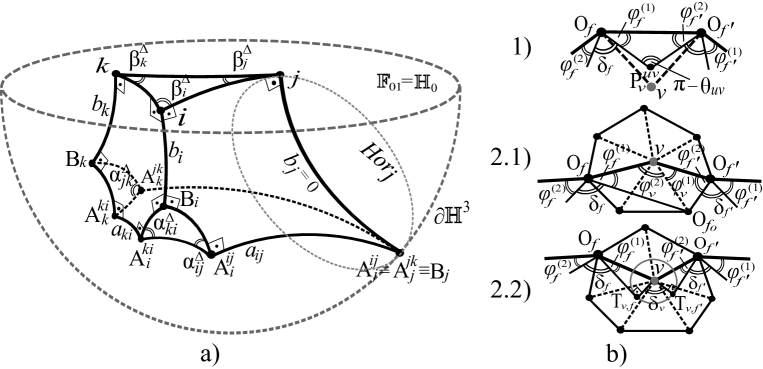
Figure 4. a) A hyper-ideal tetrahedron $\tau_{\Delta}$; b) The three different cases of edges on the boundary of an admissible domain $\Omega$.

Similarly, let $\mathbb{H}_{0}$ be a hyperbolic plane in $\mathbb{H}^{3}$. Then naturally, $\mathbb{H}_{0}$ is isometric to the hyperbolic plane $\mathbb{H}^{2}$. Again define a projection $H_{proj}:\mathbb{H}_{0}\to\partial\mathbb{H}^{3}$ by following down to the ideal boundary the geodesics orthogonal to $\mathbb{H}_{0}$ on one side of it. In the upper-half space model of $\mathbb{H}^{3}$ we can use a hyperbolic isometry to arrange for $\mathbb{H}_{0}$ to be the vertical orthogonal half-plane $\mathbb{H}_{0}=\{(x,y,z)\in\mathbb{R}^{3}\,:\,\,y=0,\,\,z>0\}$. Then $H_{proj}$ is simply the ninety-degree Euclidean rotation around the $x-$axis which rotates $\mathbb{H}_{0}$ to the horizontal half-plane $\{(x,y,0)\in\mathbb{R}^{3}\,:\,\,y>0\}\,\subset\,\partial\mathbb{H}^{3}$. The map $H_{proj}$ is depicted on figure 2b.

Use the common symbol $\mathbb{F}_{01}$ to denote both the horosphere $\mathbb{E}_{1}$ and the hyperbolic plane $\mathbb{H}_{0}$. Similarly, use the notation $F_{proj}$ for both maps $E_{proj}$ and $H_{proj}$. Now, let $\Delta=ijk$ be a decorated triangle in $\mathbb{F}^{2}$, with vertex circles $c_{i},c_{j},c_{k}$ and a face circle $c_{\Delta}$. Then without loss of generality we can think that $\Delta$ is in fact in $\mathbb{F}_{01}$. Let $\hat{\Delta}=F_{proj}(\Delta)\,\subset\,\partial\mathbb{H}^{3}$ with vertex circles $F_{proj}(c_{i}),\,F_{proj}(c_{j}),\,F_{proj}(c_{k})$ and a face circle $F_{proj}(c_{\Delta})$. Due to the nature of $F_{proj}$ (compare with figure 2b), the decorated triangle $\hat{\Delta}$ is an identical copy of $\Delta$. The edges of $\hat{\Delta}$ can be completed to either circles or straight lines. Each straight line can be extended vertically to a half-plane orthogonal to $\partial\mathbb{H}^{3}$. Thus, it gives rise to a hyperbolic plane in $\mathbb{H}^{3}$. Analogously, each circle, whether a vertex circle, the face circle or a circle coming from an edge of $\hat{\Delta}$, can be extended to a half sphere in $\mathbb{H}^{3}$, centered at a point on $\partial\mathbb{H}^{3}$. Each such half sphere is a hyperbolic plane in $\mathbb{H}^{3}$. To fix notations, for each $u\in V_{\Delta}$, the hyperbolic plane extending the projected vertex circle $F_{proj}(c_{u})$ is denoted by $\tilde{c}_{u}$ (see figure 2b) and the hyperbolic plane extending the projected face circle $F_{proj}(c_{\Delta})$ is denoted by $\tilde{c}_{\Delta}$. Furthermore, for each edge $uv\in E_{\Delta}$, the completion of $F_{proj}(uv)$ to either a straight line or a whole circle (whichever applies) extends to the hyperbolic plane $\widetilde{uv}$. As a result of this construction, to each decorated triangle $\Delta\subset\mathbb{F}_{01}$ we associate the finite set of all hyperbolic planes constructed above. In the case of $\mathbb{F}^{2}=\mathbb{H}^{2}$ we add to that set the plane $\mathbb{H}_{0}$. Subsequently, all these hyperbolic planes bound a convex hyperbolic polyhedron of finite volume, denoted by $\tau_{\Delta}$ (see figure 4a).

For each vertex $u\in V_{\Delta}$ let $B_{u}$ be the intersection point of the three hyperbolic planes $\widetilde{wu},\,\widetilde{uv}$ and $\tilde{c}_{u}$, where $u\neq v\neq w\in V_{\Delta}$. Furthermore, let $A^{uv}_{u}$ be the intersection point of the three hyperbolic planes $\tilde{c}_{\Delta},\,\tilde{c}_{u}$ and $\widetilde{uv}$, and let $A^{uv}_{v}$ be the intersection point of $\tilde{c}_{\Delta},\,\tilde{c}_{v}$ and $\widetilde{uv}$. In the case when $c_{u}$ is collapsed to a point, the hyperbolic plane $\tilde{c}_{u}$ degenerates to an ideal point, and thus the three points $B_{u},\,A^{wu}_{u}$ and $A^{uv}_{u}$ merge into one ideal point of $\tau_{\Delta}$. Also, if the vertex circles $c_{u}$ and $c_{v}$ touch, then the two points $A^{uv}_{u}$ and $A^{uv}_{v}$ become one ideal point of $\tau_{\Delta}$. When $\mathbb{F}_{01}=\mathbb{H}_{0}$, in the most general case, the polyhedron $\tau_{\Delta}$ has the combinatorics of a tetrahedron with all four vertices truncated so that the four truncating faces are disjoint triangles with no vertices in common. One of these truncating faces is the decorated triangle $\Delta=ijk\subset\mathbb{H}_{0}$. Whenever a vertex circle of the corresponding decorated triangle is shrunk to a point, the tetrahedral vertex it corresponds to is not truncated. It becomes an ideal vertex (see figure 4a). Whenever two vertex circles touch, the corresponding truncating faces share a common ideal vertex. Furthermore, when $\mathbb{F}_{01}=\mathbb{E}_{1}$, in the most general case, the polyhedron $\tau_{\Delta}$ has the combinatorics of a tetrahedron with one ideal vertex and the three remaining vertices truncated so that the three truncating faces are again disjoint triangles with no vertices in common. The rest of the cases are analogous to the ones discussed above. Notice that for $\mathbb{F}_{01}=\mathbb{E}_{1}$, the polyhedron $\tau_{\Delta}$ is decorated with the horosphere $\mathbb{E}_{1}$, which we call a decorating horosphere and the decorated triangle $\Delta=ijk$ lies on it.

Now, assume that for $u\in V_{\Delta}$ the vertex circle $c_{u}$ is a point. Then we add to the polyhedron $\tau_{\Delta}$ the unique horosphere $Hor_{u}$ tangent to $\partial\mathbb{H}^{3}$ at the ideal point $B_{u}\equiv A^{wu}_{u}\equiv A^{uv}_{u}$ and at the same time tangent to $\mathbb{F}_{01}$ at the point $u$ (as shown on figure 4a).
End of construction 7.1.

Lemma 7.1.

Let $\tau_{\Delta}$ be the polyhedron obtained from the decorated triangle $\Delta=ijk$ in $\mathbb{F}_{01}\subset\mathbb{H}^{3}$, according to construction 7.1. Then for each $u\neq v\neq w\in V_{\Delta}$ the following statements hold (see figure 4a):

1. The geodesic edge $A^{uv}_{u}A^{uv}_{v}$ of the polyhedron $\tau_{\Delta}$ is orthogonal to both truncating triangular faces $A^{wu}_{u}A^{uv}_{u}B_{u}\,\subset\,\tilde{c}_{u}$ and $A^{uv}_{v}A^{vw}_{v}B_{v}\,\subset\,\tilde{c}_{v}$. Its hyperbolic length is denoted by $a_{uv}=l_{\mathbb{H}^{3}}(A^{uv}_{u}A^{uv}_{v})$. The interior dihedral angle of $\tau_{\Delta}$ at the edge $A^{uv}_{u}A^{uv}_{v}$ is equal to the value $\alpha^{\Delta}_{uv}=\measuredangle A^{wu}_{u}A^{uv}_{u}B_{u}=\measuredangle A^{vw}_{v}A^{uv}_{v}B_{v}$.

2. The geodesic edge $uB_{u}$ of $\tau_{\Delta}$ is orthogonal to the truncating face $A^{wu}_{u}A^{uv}_{u}B_{u}\,\,\subset\,\,\tilde{c}_{u}$ and to $\mathbb{F}_{01}$. Its length is denoted by $l_{\mathbb{H}^{3}}(uB_{u})=b_{u}$. The interior dihedral angle of $\tau_{\Delta}$ at the edge $uB_{u}$ is equal to $\beta^{\Delta}_{u}=\measuredangle A^{wu}_{u}B_{u}A^{uv}_{u}=\measuredangle wuv$.

3. Let $c_{u}$ be a point. If $c_{v}$ has a non-zero radius, then the dihedral angle at the edge $A^{uv}_{u}A^{uv}_{v}$ is equal to $\alpha^{\Delta}_{uv}=\measuredangle A^{vw}_{v}A^{uv}_{v}B_{v}$ and the edge itself is perpendicular to $Hor_{u}$ and $\tilde{c}_{v}$. The oriented distance between $Hor_{u}$ and $\tilde{c}_{v}$ along the geodesic $A^{uv}_{u}A^{uv}_{v}$ is denoted by $a_{uv}$, where its sign is positive whenever $Hor_{u}$ and $\tilde{c}_{v}$ are disjoint, and negative if they intersect. If $c_{v}$ is also a point then the dihedral angle at the edge $A^{uv}_{u}A^{uv}_{v}$ is still $\alpha^{\Delta}_{uv}$ and the edge is perpendicular to both $Hor_{u}$ and $Hor_{v}$. The oriented distance between $Hor_{u}$ and $Hor_{v}$ along $A^{uv}_{u}A^{uv}_{v}$ is $a_{uv}$, with a positive sign if the two horospheres are disjoint and negative otherwise.

4. If $c_{u}$ is a point, then $b_{u}=0$. The edge $uB_{u}$ is orthogonal to $Hor_{u}$ and $\mathbb{F}_{01}$ and its interior dihedral angle is $\measuredangle wuv=\beta^{\Delta}_{u}$.

5. If $c_{u}$ and $c_{v}$ touch, then $A^{uv}_{u}\equiv A^{uv}_{v}\,\in\,\partial\mathbb{H}^{3}$ and so $a_{uv}=0$. Moreover, the dihedral angle at that ideal point is $\alpha^{\Delta}_{uv}=0$.

Proof.

The proof is a straightforward consequence of the conformal properties of the upper half-space model of $\mathbb{H}^{3}$, combined with construction 7.1 above. ∎

We fix some terminology. The edges $A^{ij}_{i}A^{ij}_{j},\,\,A^{jk}_{j}A^{jk}_{k}$ and $A^{ki}_{k}A^{ki}_{i}$, as well as the edges $iB_{i},\,jB_{j}$ and $kB_{k}$ of the polyhedron $\tau_{\Delta}$ are called principal edges. The rest of the edges are called auxiliary edges. The lengths of the principal edges are called principal edge-lengths of $\tau_{\Delta}$. For short sometimes we will also call them just edge-lengths of $\tau_{\Delta}.$ The interior dihedral angles at the principal edges are called principal dihedral angles of $\tau_{\Delta}$. For short, often we will call them simply dihedral angles of $\tau_{\Delta}$. Observe that the dihedral angles at the auxiliary edges are all equal to $\pi/2$.

Definition 7.1.

A hyper-ideal tetrahedron (see [19, 21] and figure 4a) is a geodesic polyhedron in $\mathbb{H}^{3}$ that has the combinatorics of a tetrahedron with some (possibly all) of its vertices truncated by triangular truncating faces. Each truncating face is orthogonal to the faces and the edges it truncates. Furthermore, a pair of truncating faces either do not intersect or share only one vertex. Finally, the non-truncated vertices are all ideal.

The polyhedron $\tau_{\Delta}$, constructed above, is a hyper-ideal tetrahedron. This terminology comes from the interpretation that in the Klein projective model or the Minkowski space-time model of $\mathbb{H}^{3}$ [23, 5, 21], $\tau_{\Delta}$ can be represented by an actual tetrahedron with some vertices lying outside $\mathbb{H}^{3}$ (hence the term hyper-ideal vertices). The dual to each hyper-ideal vertex is the orthogonal truncating plane.

Construction 7.2. We already know how to construct a hyper-ideal tetrahedron from a decorated triangle. Now we explain how to do the opposite. That is, we can take a hyper-ideal tetrahedron and associate to it a decorated triangle. Let $\tau$ be a hyper-ideal tetrahedron carrying the notations from construction 7.1. Then either $ijk$ is a truncating triangular face of $\tau$, defining a hyperbolic plane $\mathbb{H}_{0}$, as shown on figure 4a, or it lies on a horosphere $\mathbb{E}_{1}$ centered at an ideal vertex of $\tau$. Either way, we denote $\mathbb{H}_{0}$ and $\mathbb{E}_{1}$ with the common letter $\mathbb{F}_{01}$. If $\mathbb{F}_{01}=\mathbb{H}_{0}$ then $ijk$ is a hyperbolic triangle. If $\mathbb{F}_{01}=\mathbb{E}_{1}$ then the hyperbolic metric restricted on $\mathbb{E}_{1}$ makes $\mathbb{E}_{1}$ isometric to the Euclidean plane and the triangle $ijk$ is then a Euclidean triangle. Furthermore, each triangular truncating face $A^{wu}_{u}A^{uv}_{u}B_{u}$ determines a hyperbolic plane $\tilde{c}_{u}$ whose ideal points form a circle $c^{\infty}_{u}\,\subset\,\partial\mathbb{H}^{3}$ (see figure 2b). Similarly, the face $A^{ki}_{i}A^{ij}_{i}A^{ij}_{j}A^{jk}_{j}A^{jk}_{k}A^{ki}_{i}$ determines a hyperbolic plane $\tilde{c}_{\Delta}$, whose ideal points form a circle $c^{\infty}_{\Delta}\,\subset\,\partial\mathbb{H}^{3}$. Then the preimages $c_{i}=F^{-1}_{proj}(c^{\infty}_{i}),\,c_{j}=F^{-1}_{proj}(c^{\infty}_{j})$ and $c_{k}=F^{-1}_{proj}(c^{\infty}_{k})$ are vertex circles for $\triangle ijk$. Furthermore, $c_{\Delta}=F^{-1}_{proj}(c^{\infty}_{\Delta})$ is the corresponding face circle, orthogonal to the three vertex circles, since the face plane $\tilde{c}_{\Delta}$ of $\tau$ is by definition orthogonal to the truncating planes $\tilde{c}_{i},\tilde{c}_{j},\tilde{c}_{k}$. Because the upper half-space model is conformal, the six principal dihedral angles of $\tau$ equal the angles of the constructed decorated triangle. Observe that this construction is the converse of construction 7.1.
End of construction 7.2.

Lemma 7.2.

Let construction 7.1 produce two hyper-ideal tetrahedra $\tau_{\Delta}$ and $\tau_{\Delta}$ in $\mathbb{H}^{3}$ from two isometric (or similar if applicable) decorated triangles $\Delta$ and $\Delta^{\prime}$ in $\mathbb{F}^{2}$. Then $\tau_{\Delta}$ and $\tau_{\Delta^{\prime}}$ are isometric. Conversely, let construction 7.2 produce two decorated triangles $\Delta_{\tau}$ and $\Delta_{\tau^{\prime}}$ from two isometric hyper-ideal tetrahedra $\tau$ and $\tau^{\prime}$ in $\mathbb{H}^{3}$. Then $\Delta_{\tau}$ and $\Delta_{\tau^{\prime}}$ are isometric (or similar if applicable).

Proof.

Let $\mathbb{F}_{01}$ and $\mathbb{F}_{01}^{\prime}$ be two isometrically embedded copies of $\mathbb{F}^{2}$ in $\mathbb{H}^{3}$. Both of these are ether two hyperbolic planes or two horospheres. Without loss of generality one can think that $\Delta$ lies in $\mathbb{F}_{01}$ and $\Delta^{\prime}$ lies in $\mathbb{F}_{01}^{\prime}$. Throughout this proof $F_{proj}:\mathbb{F}_{01}\to\partial\mathbb{H}^{3}$ and $F^{\prime}_{proj}:\mathbb{F}_{01}^{\prime}\to\partial\mathbb{H}^{3}$ are the corresponding maps defined in construction 7.1 and also used in construction 7.2.

First, assume $\mathbb{F}_{01}$ and $\mathbb{F}_{01}^{\prime}$ are horospheres. In this case, the two triangles are similar. Therefore, there exists an isometry $g$ of $\mathbb{H}^{3}$ such that $g(\mathbb{F}_{01})$ and $\mathbb{F}_{01}^{\prime}$ have a common point at infinity and $g(F_{proj}(\Delta))=F^{\prime}_{proj}(\Delta^{\prime})$. Here, one invokes the property that hyperbolic isometries of $\mathbb{H}^{3}$ naturally extend to conformal automorphisms of $\partial\mathbb{H}^{3}$ (see [23, 5]). Observe that by construction 7.1, $\,g(F_{proj}(\Delta))$ and $F^{\prime}_{proj}(\Delta^{\prime})$ give rise to the two hyper-ideal tetrahedra $\tau_{g(\Delta)}$ and $\tau_{\Delta^{\prime}}$, so $\tau_{g(\Delta)}=\tau_{\Delta^{\prime}}$. Since construction 7.1 is entirely defined in terms of the geometry of $\mathbb{H}^{3}$, it commutes with $\mathbb{H}^{3}-$isometries, i.e. $\tau_{g(\Delta)}=g(\tau_{\Delta})$. Hence $g(\tau_{\Delta})=\tau_{\Delta^{\prime}}$, i.e. $\tau_{\Delta}$ and $\tau_{\Delta^{\prime}}$ are isometric.

Next, let us assume that $\mathbb{F}_{01}$ and $\mathbb{F}_{01}^{\prime}$ are hyperbolic planes. Then $\Delta$ and $\Delta^{\prime}$ are isometric. Therefore, there exists and isometry $g\in Isom(\mathbb{H}^{3})$ such that $g(\mathbb{F}_{01})=\mathbb{F}_{01}^{\prime}$, $\,g(\Delta)=\Delta^{\prime}$ and $g$ maps the side of $\mathbb{F}_{01}$ on which $F_{proj}$ is defined to the side of $\mathbb{F}_{01}^{\prime}$ on which $F_{proj}^{\prime}$ is defined. Again, since construction 7.1 is purely geometric, $g\circ F_{proj}=F^{\prime}_{proj}\circ g$. Therefore, $g(F_{proj}(\Delta))=F^{\prime}_{proj}(g(\Delta))=F^{\prime}_{proj}(\Delta^{\prime})$. By construction 7.1 $\,\tau_{\Delta^{\prime}}=\tau_{g(\Delta)}=g(\tau_{\Delta})$, i.e. $\tau_{\Delta}$ and $\tau_{\Delta^{\prime}}$ are isometric.

Conversely, let $\tau$ and $\tau^{\prime}$ be two hyper-ideal tetrahedra in $\mathbb{H}^{3}$ and $g\in Isom(\mathbb{H}^{3})$ be a hyperbolic isometry, such that $g(\tau)=\tau^{\prime}$.

If $\mathbb{F}^{2}=\mathbb{H}^{2}$ then $\tau$ and $\tau^{\prime}$ have a pair of triangular truncating faces $\Delta$ and $\Delta^{\prime}$ respectively, where $\Delta^{\prime}=g(\Delta)$. The faces $\Delta$ and $\Delta^{\prime}$ define the hyperbolic planes $\mathbb{F}_{01}\supset\Delta$ and $\mathbb{F}_{01}^{\prime}\supset\Delta^{\prime}$ respectively, thus $\mathbb{F}_{01}^{\prime}=g(\mathbb{F}_{01})$. Construction 7.2 makes $\Delta$ into a decorated triangle $\Delta_{\tau}$ and $\Delta^{\prime}$ into a decorated triangle $\Delta_{\tau^{\prime}}$. Since construction 7.2 is purely geometric in nature, it commutes with $g$. In other words, $\Delta_{\tau^{\prime}}=\Delta_{g(\tau)}=g(\Delta_{\tau})$, i.e. the decorated triangles $\Delta_{\tau^{\prime}}$ and $\Delta_{\tau}$ are isometric.

Finally, let $\mathbb{F}^{2}=\mathbb{E}^{2}$. Then $\tau$ and $\tau^{\prime}$ have a corresponding pair of ideal vertices $\infty$ of $\tau$ and $\infty^{\prime}\in\partial\mathbb{H}^{3}$ of $\tau^{\prime}$ such that $g(\infty)=\infty^{\prime}$. There are two horospheres $\mathbb{F}_{01}$ and $\mathbb{F}_{01}^{\prime}$ of $\tau$ respectively tangent to $\partial\mathbb{H}^{3}$ at these two points. Construction 7.2 produces two decorated triangles $\Delta_{\tau}\subset\mathbb{F}_{01}$ and $\Delta_{\tau^{\prime}}\subset\mathbb{F}_{01}^{\prime}$. Observe, that in this case $g(\Delta_{\tau})$ might not be equal to $\Delta_{\tau^{\prime}}$ because $g(\mathbb{F}_{01})$ might not be equal to $\mathbb{F}_{01}^{\prime}$. Instead, in general we have two horospheres $\mathbb{F}_{01}^{\prime}$ and $\mathbb{F}_{01}^{\prime\prime}=g(\mathbb{F}_{01})$ tangent to infinity at the same ideal vertex $\infty^{\prime}$. As pointed out already, construction 7.2 commutes with $g$, so $g(\Delta_{\tau})=\Delta_{g(\tau)}^{\prime\prime}=\Delta_{\tau^{\prime}}^{\prime\prime}$, where the decorated triangle $\Delta_{\tau^{\prime}}^{\prime\prime}$ is the result of construction 7.2 on the horosphere $\mathbb{F}_{01}^{\prime\prime}$ with respect to $\tau^{\prime}$. Now, shifting the horosphere $\mathbb{F}_{01}^{\prime\prime}$ to the horosphere $\mathbb{F}_{01}^{\prime}$ slides the decorated triangle $\Delta_{\tau^{\prime}}^{\prime\prime}$ onto $\mathbb{F}_{01}^{\prime}$ so that it matches the decorated triangle $\Delta_{\tau^{\prime}}$. As the restriction of $g$ onto $\mathbb{F}_{01}$ is an Euclidean isometry between $\mathbb{F}_{01}$ and $\mathbb{F}_{01}^{\prime\prime}$, and the shifting of $\mathbb{F}_{01}^{\prime\prime}$ onto $\mathbb{F}_{01}^{\prime}$ is scaling, the two decorated triangles $\Delta_{\tau^{\prime}}$ and $\Delta_{\tau}$ are similar. ∎

Proposition 7.1.

Each hyper-ideal tetrahedron in $\mathbb{H}^{3}$ is defined uniquely up to isometry by its six principal dihedral angles, belonging to the set $\mathcal{A}_{\Delta}$.

Proof.

The principal dihedral angles of a hyper-ideal tetrahedron are also the angles of its corresponding decorated triangle obtained by construction 7.2, so they belong to $\mathcal{A}_{\Delta}$. Conversely, assume we are given a vector of six numbers $(\alpha^{\Delta},\beta^{\Delta})$ from $\mathcal{A}_{\Delta}$. Proposition 5.5 allows us to construct a decorated triangle with $(\alpha^{\Delta},\beta^{\Delta})$ as angles. Construction 7.1 allows us to extend the decorated triangle to a hyper-ideal tetrahedron with $(\alpha^{\Delta},\beta^{\Delta})$ as principal dihedral angles, a fact established in lemma 7.1. In order to prove uniqueness, let $(\alpha^{\Delta},\beta^{\Delta})$ give rise to two hyper-ideal tetrahedra. Then by construction 7.2 these two tetrahedra correspond to two decorated triangles with equal angles. By proposition 5.5, the two decorated triangles are isometric (or similar). Therefore, by lemma 7.2, and the fact that constructions 7.1 and 7.2 are converse to each other, the two tetrahedra are isometric.∎

Consequently, we can geometrize a combinatorial triangle in two ways. We can either turn it into a decorated triangle or we can turn it into a hyper-ideal tetrahedron. The association with hyper-ideal tetrahedra will provide us with the right quantitative description of the space of generalized hyper-ideal circle patterns. Given a tetrahedron $\tau_{\Delta}$ arising from a decorated triangle $\Delta=ijk$ via construction 7.1, we can extract the six principal edge-lengths $(a,b)_{\Delta}=\big{(}a_{ij},a_{jk},a_{ki},b_{k},b_{i},b_{j}\big{)}\in\mathbb{R}^{E_{\Delta}}\times\mathbb{R}^{V_{\Delta}}$. Recall that these are the numbers determined in lemma 7.1 (see also figure 4a). Notice that some of them could be zero. Given a combinatorial triangle $\Delta=ijk$, define the space of tetrahedral edge-lengths $\mathcal{TE}_{\Delta}$ to be the set of all six numbers $\big{(}a_{ij},a_{jk},a_{ki},b_{k},b_{i},b_{j}\big{)}$ which are the principal edge-lengths of hyper-ideal tetrahedrons with fixed combinatorics provided by $\Delta$.

Our goal is to describe generalized hyper-ideal circle patterns in terms of principal edge-lengths of the corresponding tetrahedra. For the topological triangulation $\mathcal{T}=(V,E_{T},F_{T})$ on the surface $S$ assign to its edges $a:E_{T}\to\mathbb{R}$ and to its vertices $b:V\to\mathbb{R}$ so that for each face $\Delta\in F_{T}$ the six numbers $(a,b)_{\Delta}$, with possible zeroes among them, are principal edge-lengths of a hyper-ideal tetrahedron $\tau_{\Delta}$. Thus, one can define the space $\mathcal{TE}$ as the set of all assignments $(a,b)\in\mathbb{R}^{E_{\pi}\cup E_{1}}\times\mathbb{R}^{V_{1}}\,\subset\,\mathbb{R}^{E_{T}}\times\mathbb{R}^{V}$ such that for any $\Delta\in F_{T}$ the six numbers $(a,b)_{\Delta}$, some of which could be fixed to be zero, belong to $\mathcal{TE}_{\Delta}$.

Lemma 7.3.

Let $\Delta=ijk$ be a decorated triangle in $\mathbb{F}^{2}\cong\mathbb{F}_{01}$ and let $\tau_{\Delta}$ be its corresponding hyper-ideal tetrahedron (see constructions 7.1 and 7.2, as well as figure 4a). Let $(l,r)_{\Delta}=\big{(}l_{ij},l_{jk},l_{ki},r_{k},r_{i},r_{j}\big{)}\in\mathcal{ER}_{\Delta}$ be the the three edge-lengths and three vertex radii of $\Delta$, and let $(a,b)_{\Delta}=\big{(}a_{ij},a_{jk},a_{ki},b_{k},b_{i},b_{j}\big{)}\in\mathcal{TE}_{\Delta}$ be the six principal edge-lengths of $\tau_{\Delta}$. Then for $v\in V_{\Delta}$ and $uv\in E_{\Delta}$ the following formulas hold:

1. $\mathbb{F}^{2}=\mathbb{E}^{2}$.

$$r_{v} =e^{-b_{v}}\,\,\text{ if }\,\,v\in V_{1}\,\,\,\,\text{ and }\,\,\,\,r_{v}=b_{v}=0\,\,\text{ if }\,\,v\in V_{0}$$ (7)

$$l_{uv} =\sqrt{e^{-2b_{u}}+e^{-2b_{v}}+2e^{-b_{u}-b_{v}}\cosh{a_{uv}}}\,\,\,\,\text{ if }\,\,uv\in E_{1}\cup E_{\pi}\,\text{ and }\,u,v\in V_{1}$$ (8)

$$l_{uv} =\sqrt{e^{-2b_{v}}+e^{a_{uv}-b_{v}}}\,\,\,\,\text{ if }\,\,uv\in E_{1}\cup E_{\pi}\,\,\text{ and }\,\,u\in V_{0},\,\,v\in V_{1}$$ (9)

$$l_{uv} =e^{a_{uv}/2}\,\,\text{ if }\,\,\,\,uv\in E_{1}\cup E_{\pi}\,\,\text{ and }\,\,u,v\in V_{0}$$ (10)

$$l_{uv} =e^{-b_{u}}+e^{-b_{v}}\,\,\,\,\text{ if }\,\,uv\in E_{0}$$ (11)

2. $\mathbb{F}^{2}=\mathbb{H}^{2}$.

$$r_{v} =\sinh^{-1}{\Big{(}\frac{1}{\sinh{b_{v}}}\Big{)}}\,\,\text{ if }\,\,v\in V_{1}\,\,\,\,\text{ and }\,\,\,\,r_{v}=b_{v}=0\,\,\text{ if }\,\,v\in V_{0}$$ (12)

$$l_{uv} =\cosh^{-1}{\Big{(}\frac{\cosh{a_{uv}}+\cosh{b_{u}}\cosh{b_{v}}}{\sinh{b_{u}}\sinh{b_{v}}}\Big{)}}\,\,\,\,\text{ if }\,\,uv\in E_{1}\cup E_{\pi}\,\text{ and }\,u,v\in V_{1}$$ (13)

$$l_{uv} =\cosh^{-1}{\Big{(}\frac{e^{a_{uv}}+\cosh{b_{v}}}{\sinh{b_{v}}}\Big{)}}\,\,\,\,\text{ if }\,\,uv\in E_{1}\cup E_{\pi}\,\,\text{ and }\,\,u\in V_{0},\,\,v\in V_{1}$$ (14)

$$l_{uv} =2\sinh^{-1}{\big{(}e^{a_{uv}/2}\big{)}}\,\,\,\,\text{ if }\,\,uv\in E_{1}\cup E_{\pi}\,\,\text{ and }\,\,u,v\in V_{0}$$ (15)

$$l_{uv} =\sinh^{-1}{\Big{(}\frac{1}{\sinh{b_{u}}}\Big{)}}+\sinh^{-1}{\Big{(}\frac{1}{\sinh{b_{v}}}\Big{)}}\,\,\,\,\text{ if }\,\,uv\in E_{0}.$$ (16)

Proof.

Constructions 7.1 and 7.2 reveal that both six-tuples $(l,r)_{\Delta}$ and $(a,b)_{\Delta}$ are naturally assigned to the same polyhedron $\tau_{\Delta}$ (figure 4a). Then, for any $uv\in E_{\Delta}$, the face that contains the points $uB_{u}A^{uv}_{u}A^{uv}_{v}B_{v}v$ can be treated as a geodesic polygon in $\mathbb{H}^{2}$. Observe that some of the points that determine the face may actually merge together into ideal points. First, one can derive formulas (7) by a direct integration in the upper half-plane. Equality (12) comes from a standard formula from hyperbolic trigonometry (see [9]). Then, in order to derive the rest of the expressions from the list (7) - (16), one could look at the face $uB_{u}A^{uv}_{u}A^{uv}_{v}B_{v}v$ and simply apply various formulas from hyperbolic trigonometry to express the length $l_{uv}=l_{\mathbb{H}^{2}}(uv)$ as a function of the given lengths $a_{uv},b_{u}$ and $b_{v}$. For instance, (13) follows from the hyperbolic law of cosines for a right-angled hexagon, while (14) and (15) could be respectively interpreted as the reduction of that cosine law to right-angled pentagons with one ideal vertex and to right-angled quadrilaterals with two ideal vertices. In fact most of the equalities (7) - (16) could be found in the texts [9, 5, 23, 21]. Those that might not be easy to come across in the literature could be derived by combining the hyperbolic geometry of the upper half-plane model with the underlying Euclidean geometry. ∎

Recall that in the case of $\mathbb{F}^{2}=\mathbb{E}^{2}$, decorated triangles are considered up to Euclidean motions and scaling. In the polyhedral interpretation, the corresponding hyper-ideal tetrahedra come decorated with a choice of a horosphere $\mathbb{E}_{1}$. The rescaling of the Euclidean decorated triangle corresponds to a shift of $\mathbb{E}_{1}$ closer to or further from its ideal vertex. If there are other ideal vertices, their horoshperes $Hor_{u}$ are adjusted accordingly. This rescaling manifests itself as a free $\mathbb{R}-$action on both spaces $\mathcal{TE}$ and $\mathcal{TE}_{\Delta}$. For $t\in\mathbb{R},$ the actions $(a,b)\mapsto ACT_{t}(a,b)$ and $(a,b)_{\Delta}\mapsto ACT^{\Delta}_{t}(a,b)$ are expressed with the formulas

$$b_{k}\mapsto b_{k}-t\,\,\,\,\text{ if }\,k\in V_{1}$$

$$a_{ij}\mapsto a_{ij}+t\,\,\,\,\text{ if }i\in V_{0},\,j\in V_{1}$$

$$a_{ij}\mapsto a_{ij}+2t\,\,\,\,\text{ if }i,\,j\in V_{0}.$$

To factor out the $\mathbb{R}-$action define the cross-sections

$$\mathcal{TE}_{0} =\Big{\{}(a,b)\in\mathcal{TE}\,\,\big{|}\,\,\sum_{i\text{ or }j\in V_{0}}a_{ij}-\sum_{k\in V_{1}}b_{k}=0\,\,\Big{\}}$$

$$\mathcal{TE}_{0,\Delta} =\Big{\{}(a,b)_{\Delta}\in\mathcal{TE}_{\Delta}\,\,\big{|}\,\,\sum_{i\text{ or }j\in V^{0}_{\Delta}}a_{ij}-\sum_{k\in V_{\Delta}^{1}}b_{k}=0\,\,\Big{\}}.$$

In the case $\mathbb{F}^{2}=\mathbb{H}^{2}$, we simply take $\mathcal{TE}_{0}=\mathcal{TE}$ and $\mathcal{TE}_{0,\Delta}=\mathcal{TE}_{\Delta},$ i.e. we assume that the $\mathbb{R}-$action is trivial. Let $PR:\mathcal{TE}\to\mathcal{TE}_{0}$ and $PR_{\Delta}:\mathcal{TE}_{\Delta}\to\mathcal{TE}_{0,\Delta}$ be the linear projection maps along the orbits of $\mathbb{R}$. When $\mathbb{F}^{2}=\mathbb{H}^{2}$, the maps $PR$ and $PR_{\Delta}$ are actually the identity, because $\mathbb{R}$ acts trivially. When $\mathbb{F}^{2}=\mathbb{E}^{2}$, the maps $PR$ and $PR_{\Delta}$ are linear maps with one dimensional kernels. Recall that whenever $\mathbb{F}^{2}=\mathbb{E}^{2}$, $\,\mathbb{R}$ also acts on $\mathcal{ER}$ and $\mathcal{ER}_{\Delta}$ by $(l,r)\mapsto(e^{t}l,e^{t}r)$ and $(l,r)_{\Delta}\mapsto(e^{t}l,e^{t}r)_{\Delta}$ respectively. In the case $\mathbb{F}^{2}=\mathbb{H}^{2}$, we can again assume that $\mathbb{R}$ acts trivially. Either way, denote these actions by $(l,r)\mapsto E_{t}(l,r)$ and $(l,r)_{\Delta}\mapsto E^{\Delta}_{t}(l,r)$.

Lemma 7.4.

There are real analytic diffeomorphisms $\tilde{\Psi}\,:\,\mathcal{TE}\,\to\,\mathcal{ER}$ and $\tilde{\Psi}_{\Delta}\,:\,\mathcal{TE}_{\Delta}\,\to\,\mathcal{ER}_{\Delta}$, defined by the formulas in lemma 7.3. Geometrically speaking, $\tilde{\Psi}_{\Delta}$ maps the principal edge-lengths of a hyper-ideal tetrahedron with combinatorics $\Delta$ to the edge-lengths and vertex radii of its corresponding decorated triangle (see constructions 7.1 and 7.2). Furthermore, $\tilde{\Psi}\circ ACT_{t}=E_{t}\circ\tilde{\Psi}$ and $\tilde{\Psi}_{\Delta}\circ ACT^{\Delta}_{t}=E^{\Delta}_{t}\circ\Psi_{\Delta}$. Consequently, there is a pair of real analytic diffeomorphisms $\Psi\,:\,\mathcal{TE}_{0}\,\to\,\mathcal{ER}_{1}$ and $\Psi_{\Delta}\,:\,\mathcal{TE}_{0,\Delta}\,\to\,\mathcal{ER}_{1,\Delta}$. Finally, $\mathcal{TE}=\tilde{\Psi}^{-1}(\mathcal{ER})$ and $\mathcal{TE}_{0}=\Psi^{-1}(\mathcal{ER}_{1})$ as well as $\mathcal{TE}_{\Delta}=\tilde{\Psi}^{-1}_{\Delta}(\mathcal{ER}_{\Delta})$ and $\mathcal{TE}_{0,\Delta}=\Psi^{-1}_{\Delta}(\mathcal{ER}_{1,\Delta})$.

Proof.

The geometric interpretation follows from lemma 7.3. The formulas from lemma 7.3 are real analytic expressions, so the maps $\tilde{\Psi}$ and $\tilde{\Psi}_{\Delta}$ are real analytic. It is straightforward to invert formulas (7) and (12) and express $b_{v}$ as a function of $r_{v}$. After that, one can easily invert the rest of the formulas and express $a_{uv}$ in terms of $r_{u},r_{v}$ and $l_{uv}$ explicitly. Thus, one obtains well defined real analytic expressions, which define the inverse maps $\tilde{\Psi}^{-1}$ and $\tilde{\Psi}_{\Delta}^{-1}$. Furthermore, having in mind how $\mathbb{R}$ acts on the spaces $\mathcal{TE}$ and $\mathcal{ER}$ (resp. $\mathcal{TE}_{\Delta}$ and $\mathcal{ER}_{\Delta}$), it is straight forward to check the $\mathbb{R}-$equivariance of the maps $\tilde{\Psi}$ and $\tilde{\Psi}_{\Delta}$. Finally, one can define $\Psi$ and $\Psi_{\Delta}$ so that $\Psi^{-1}=PR\circ\tilde{\Psi}^{-1}|_{\mathcal{ER}_{1}}\,:\,\mathcal{ER}_{1}\,\to\,\mathcal{TE}_{0}$ and $\Psi^{-1}_{\Delta}=PR_{\Delta}\circ\tilde{\Psi}^{-1}_{\Delta}|_{\mathcal{ER}_{1}}\,:\,\mathcal{ER}_{1,\Delta}\,\to\,\mathcal{TE}_{0,\Delta}$. ∎

Proposition 7.2.

A hyper-ideal tetrahedron in $\mathbb{H}^{3}$ is defined uniquely up to isometry by its principal edge-lengths, belonging to the set $\mathcal{TE}_{0,\Delta}$.

Proof.

By definition, the principal edge-lengths of a hyper-ideal tetrahedron belong to $\mathcal{TE}_{\Delta}$. If given edge-lengths $(a,b)_{\Delta}\in\mathcal{TE}_{0,\Delta}$, then take $(l,r)_{\Delta}=\Psi_{\Delta}(a,b)\in\mathcal{ER}_{1,\Delta}$. Choose an arbitrary $\mathbb{F}_{01}\subset\mathbb{H}^{3}$ and by proposition 6.1 construct in $\mathbb{F}_{01}$ a decorated triangle with edge-lengths and vertex radii $(l,r)_{\Delta}$. Then apply construction 7.1 to obtain a hyper-ideal tetrahedron. By lemma 7.4 the tetrahedron has principal edge-lengths $(a,b)_{\Delta}\in\mathcal{TE}_{0,\Delta}$. In order to prove uniqueness, let $(a,b)_{\Delta}\in\mathcal{TE}_{0,\Delta}$ give rise to two hyper-ideal tetrahedra. Then by construction 7.2 these two tetrahedra correspond to two decorated triangles with equal edge-lengths and vertex radii. By proposition 6.1, the two decorated triangles are isometric. Therefore, by lemma 7.2, and the fact that constructions 7.1 and 7.2 are converse to each other, the two tetrahedra are isometric. ∎

Lemma 7.5.

For a given combinatorial triangle $\Delta$, there exists an $\mathbb{R}-$invariant real analytic map $\tilde{\Phi}_{\Delta}\,:\,\mathcal{TE}_{\Delta}\,\to\,\mathcal{A}_{\Delta}$ such that its restriction $\tilde{\Phi}_{\Delta}|_{\mathcal{TE}_{0,\Delta}}=\Phi_{\Delta}\,:\,\mathcal{TE}_{0,\Delta}\,\to\,\mathcal{A}_{\Delta}$ is a real analytic diffeomorphism. The maps $\tilde{\Phi}_{\Delta}$ and $\Phi_{\Delta}$ associate to the tetrahedral edge-lengths $(a,b)_{\Delta}\in\mathcal{TE}_{0,\Delta}$ of a hyper-ideal tetrahedron with combinatorics $\Delta$ its corresponding dihedral angles $(\alpha^{\Delta},\beta^{\Delta})\in\mathcal{A}_{\Delta}$. In particular, the angles $\alpha^{\Delta}_{ij}=\alpha_{ij}^{\Delta}(a,b)$ for $ij\in E_{\Delta}$ and $\beta^{\Delta}_{k}=\beta_{k}^{\Delta}(a,b)$ for $k\in V_{\Delta}$ are $\mathbb{R}-$invariant and depend analytically on the edge-length variables $(a,b)_{\Delta}\in\mathcal{TE}_{\Delta}$ and can be written explicitly in terms of compositions of hyperbolic trigonometric formulas.

Proof.

Let $(a,b)_{\Delta}\in\mathcal{TE}_{0,\Delta}$. By applying proposition 7.2, take a hyper-ideal tetrahedron $\tau_{\Delta}$ whose principal edge-lengths are $(a,b)_{\Delta}$ and record its six angles $(\alpha^{\Delta},\beta^{\Delta})\in\mathcal{A}_{\Delta}$. Denote this map by $\Phi_{\Delta}(a,b)=(\alpha^{\Delta},\beta^{\Delta})$. Proposition 7.2 guarantees the correctness of the map’s definition, because if we choose another tetrahedron $\tau^{\prime}_{\Delta}$ with the same principal edge-lengths, its principal dihedral angles will also be $(\alpha^{\Delta},\beta^{\Delta})\in\mathcal{A}_{\Delta}$ since $\tau_{\Delta}$ and $\tau^{\prime}_{\Delta}$ have to be isometric. Furthermore, proposition 7.1 implies that $\Phi_{\Delta}\,:\,\mathcal{TE}_{0,\Delta}\,\to\,\mathcal{A}_{\Delta}$ has a well defined inverse $\Phi_{\Delta}^{-1}\,:\,\mathcal{A}_{\Delta}\,\to\,\mathcal{TE}_{0,\Delta}$. The interpretation of $(\alpha^{\Delta},\beta^{\Delta})$ as the principal dihedral angles of a hyper-ideal tetrahedron and $(a,b)_{\Delta}$ as the corresponding principal edge-lengths of the same tetrahedron follows immediately form the construction of the map $\Phi_{\Delta}$. The map $\tilde{\Phi}_{\Delta}$ is defined as $\tilde{\Phi}_{\Delta}=\Phi_{\Delta}\circ PR_{\Delta}.$ Recall that in the hyperbolic case, $RP_{\Delta}$ is the identity and so $\tilde{\Phi}_{\Delta}=\Phi_{\Delta}$.

Next, one needs so show that both $\Phi_{\Delta}$ and $\Phi^{-1}_{\Delta}$ depend analytically on their respective variables. This simply means that it is enough to make sure that the angles can be expressed as real analytic function of the edge-lengths and vice versa. This follows directly from hyperbolic trigonometry and the fact that the dependence in each direction can be written down explicitly. To illustrate this fact, we work out only one case in detail. The rest are analogous. In addition to the exposition that follows, we encourage the reader to look at figure 4a and follow the notations there.

Before we continue, we would like to emphasize that there are several alternative ways of writing down the analytic dependence of the dihedral angles on the edge-lengths and vice versa in terms of compositions of different hyperbolic trigonometric formulas (such as the hyperbolic law of sines and the various cases of the hyperbolic laws of cosines). However, we are presenting just one of them, while all the rest yield the same results, simply written down as combinations of different formulas.

Let $\tau_{\Delta}$ be a hyper-ideal tetrahedron with principal edge-lengths $(a,b)_{\Delta}$ and dihedral angles $(\alpha^{\Delta},\beta^{\Delta})$. Moreover, let $\tau_{\Delta}$ be labelled as in construction 7.1 and figure 4a. Furthermore, assume that $\tau_{\Delta}$ has one ideal vertex $A^{ij}_{j}\equiv A^{jk}_{j}\equiv B_{j}\in\partial\mathbb{H}^{3}$ and three triangular truncating faces without ideal vertices (figure 4a). Therefore $b_{j}=0$ and $\alpha^{\Delta}_{ij}+\beta^{\Delta}_{j}+\alpha^{\Delta}_{jk}=\pi$. Let $\zeta_{14}(a_{uv},b_{v})$ and $\zeta_{13}(a_{uv},b_{u},b_{v})$ be the respective right hand sides of equations (14) and (13) from lemma 7.3. Then, according to lemma 7.3, the edge lengths of the triangular face $ijk$ are

$$l_{ij}=\zeta_{14}(a_{ij},b_{i}),\,\,\,\,l_{jk}=\zeta_{14}(a_{jk},b_{k}),\,\,\,\,l_{ki}=\zeta_{13}(a_{ki},b_{k},b_{i}).$$

For an arbitrary geodesic triangle with edge-lengths $x_{1},x_{2},x_{3}$ and an angle $\gamma_{3}$ opposite to $x_{3}$, the hyperbolic law of cosines in terms of edges (see [9]) gives the formula

$$\gamma_{3}=\zeta(x_{1},x_{2},x_{3})=\arccos{\Big{(}\frac{\cosh{x_{1}}\cosh{x_{2}}-\cosh{x_{3}}}{\sinh{x_{1}}\sinh{x_{2}}}\Big{)}}.$$

Applying this equality to the triangle $\triangle ijk$, one obtains the expressions

$$\beta^{\Delta}_{i}=\zeta(l_{ki},l_{ij},l_{jk}),\,\,\,\,\beta^{\Delta}_{j}=\zeta(l_{ij},l_{jk},l_{ki}),\,\,\,\,\beta^{\Delta}_{k}=\zeta(l_{jk},l_{ki},l_{ij}).$$

Thus, the angles $\beta^{\Delta}_{i},\beta^{\Delta}_{j}$ and $\beta^{\Delta}_{k}$ are analytic functions with respect to the variables $(a,b)_{\Delta}$.

For any permutation $u\neq v\neq w\in V_{\Delta}$ such that $v\neq j$, define the lengths $\sigma^{vw}_{v}=l_{\mathbb{H}^{3}}(A^{vw}_{v}B_{v})$ and $\sigma_{v}=l_{\mathbb{H}^{3}}(A^{uv}_{v}A^{vw}_{v}).$ Since the face $iB_{i}A^{ki}_{i}A^{ki}_{k}B_{k}k$ is a right-angled hexagons, one finds $\sigma^{ki}_{i}=\zeta_{13}(b_{k},a_{ki},b_{i})$. Furthermore, the face $iB_{i}A^{ij}_{i}B_{j}j$ is a right-angled pentagon with ideal vertex $B_{j}\equiv A^{ij}_{j}\equiv A^{jk}_{j}$. Then $\sigma^{ij}_{i}=\zeta_{14}(-a_{ij},b_{i})$. Analogously, by considering the right-angled pentagon $A^{ki}_{i}A^{ij}_{i}B_{j}A^{jk}_{k}A^{ki}_{k}$ with ideal vertex $B_{j}$, one comes to the equality $\sigma_{i}=\zeta_{14}(a_{jk}-a_{ij},\,a_{ki})$. By applying the hyperbolic law of sines (see [9]) to the triangular face $A^{ki}_{i}A^{ij}_{i}B_{i}$ one comes to the expressions

$$\alpha^{\Delta}_{ij}=\arcsin{\left(\frac{\sinh{\sigma^{ki}_{i}}}{\sinh{\sigma_{i}}}\sin{\beta^{\Delta}_{i}}\right)}\,\,\,\,\text{ and }\,\,\,\,\alpha^{\Delta}_{ki}=\arcsin{\left(\frac{\sinh{\sigma^{ij}_{i}}}{\sinh{\sigma_{i}}}\sin{\beta^{\Delta}_{i}}\right)}$$

which are real analytic functions with respect to $(a,b)_{\Delta}$. Subsequently, $\alpha^{\Delta}_{jk}=\pi-\alpha^{\Delta}_{ij}-\beta^{\Delta}_{j}$ is also a real analytic function with respect to $(a,b)_{\Delta}.$

Next, we express the edge-lengths in terms of the dihedral angles. For that we need the law of cosines for a hyperbolic triangle in terms of its angles [9]

$$x_{3}=\nu(\gamma_{1},\gamma_{2},\gamma_{3})=\cosh^{-1}{\Big{(}\frac{\cos{\gamma_{1}}\cos{\gamma_{2}}+\cos{\gamma_{3}}}{\sin{\gamma_{1}}\sin{\gamma_{2}}}\Big{)}},$$

where $\gamma_{1},\gamma_{2}$ and $\gamma_{3}$ are the angles of the triangle and $x_{3}$ is the length of the edge opposite to $\gamma_{3}$. Applying this formula to the triangle $\triangle ijk$

$$l_{ij}=\nu(\beta^{\Delta}_{i},\beta^{\Delta}_{j},\beta^{\Delta}_{k}),\,\,\,\,l_{jk}=\nu(\beta^{\Delta}_{j},\beta^{\Delta}_{k},\beta^{\Delta}_{i}),\,\,\,\,l_{ki}=\nu(\beta^{\Delta}_{k},\beta^{\Delta}_{i},\beta^{\Delta}_{j}).$$

By applying the same argument to the triangles $\triangle A^{ki}_{i}A^{ij}_{i}B_{i}$ and $\triangle A^{jk}_{k}A^{ki}_{k}B_{k}$ one obtains the respective formulas

$$\sigma^{ij}_{i} =\nu(\beta^{\Delta}_{i},\alpha^{\Delta}_{ij},\alpha^{\Delta}_{ki}),\,\,\,\,\,\sigma^{ki}_{i}=\nu(\beta^{\Delta}_{i},\alpha^{\Delta}_{ki},\alpha^{\Delta}_{ij})\,\,\,\,\text{ and }$$

$$\sigma^{jk}_{k} =\nu(\beta^{\Delta}_{k},\alpha^{\Delta}_{jk},\alpha^{\Delta}_{ki}),\,\,\,\,\,\sigma^{ki}_{k}=\nu(\beta^{\Delta}_{k},\alpha^{\Delta}_{ki},\alpha^{\Delta}_{jk})$$

Since $iB_{i}$ and $A^{ki}_{i}A^{ki}_{k}$ are edges of the right-angled hexagon $iB_{i}A^{ki}_{i}A^{ki}_{k}B_{k}k$, the equalities $b_{i}=\zeta_{13}(\sigma^{ki}_{k},l_{ki},\sigma^{ki}_{i})$ and $a_{ki}=\zeta_{13}(l_{ki},\sigma^{ki}_{i},\sigma^{ki}_{k})$ hold. Same argument can be used to find $b_{k}$. However, we present a different formula, which could be useful in the case of hyper-ideal tetrahedra of other combinatorial types. For the right-angled pentagon $kB_{k}A^{jk}_{k}B_{j}j$ with one ideal vertex $B_{j}$ the following law of cosines applies [9]:

$$b_{k}=\cosh^{-1}{\left(\frac{\cosh{l_{jk}}\cosh{\sigma^{jk}_{k}}+1}{\sinh{l_{jk}}\sinh{\sigma^{jk}_{k}}}\right)}.$$

Thus, the edge-lengths $b_{i}$ and $b_{k}$ are real analytic functions with respect to the dihedral angles $(\alpha^{\Delta},\beta^{\Delta}).$ So is $b_{j}\equiv 0$. Considering the pentagonal faces $iB_{i}A^{ij}_{i}B_{j}j$ and $kB_{k}A^{jk}_{k}B_{j}j$, one can invert formula (14) in order to obtain

$$a_{ij}=\log{\big{(}\cosh{l_{ij}}\sinh{b_{i}}-\cosh{b_{i}}\big{)}}\,\,\text{ and }\,\,a_{jk}=\log{\big{(}\cosh{l_{ij}}\sinh{b_{i}}-\cosh{b_{i}}\big{)}}.$$

∎

8. Volumes of hyper-ideal tetrahedra

Assume we are given a combinatorial triangle $\Delta=ijk$. For $\mathbb{F}^{2}=\mathbb{H}^{2}$ define the affine injective map $J_{\Delta}\,:\,\mathbb{R}^{E_{\Delta}^{1}}\times\mathbb{R}^{V_{\Delta}^{1}}\,\to\,\mathbb{R}^{E_{\Delta}}\times\mathbb{R}^{V_{\Delta}}$ by

$$\beta^{\Delta}_{v} =\tilde{\beta}^{\Delta}_{v}\,\,\,\,\text{ for }\,\,v\in V_{\Delta}^{1}$$

$$\beta^{\Delta}_{v} =\pi-\tilde{\alpha}^{\Delta}_{uv}-\tilde{\alpha}^{\Delta}_{vw}\,\,\,\,\text{ for }\,\,v\in V_{\Delta}^{0}$$ (17)

$$\alpha^{\Delta}_{uv} =\tilde{\alpha}^{\Delta}_{uv}\,\,\,\,\text{ for }uv\in E_{\Delta}^{1}$$

$$\alpha^{\Delta}_{uv} =0\,\,\,\,\text{ for }uv\in E_{\Delta}^{0},$$

where $u\neq v\neq w\in V_{\Delta}$. For the case $\mathbb{F}^{2}=\mathbb{E}^{2}$, let us first exclude the case of $V^{0}_{\Delta}=V_{\Delta}$ . Thus, without loss of generality, we may assume that $k\in V_{\Delta}^{1}$ and $V_{k,\Delta}^{1}=V_{\Delta}^{1}\setminus\{k\}$. The corresponding affine injective map $J_{\Delta}\,:\,\mathbb{R}^{E_{\Delta}^{1}}\times\mathbb{R}^{V_{k,\Delta}^{1}}\,\to\,\mathbb{R}^{E_{\Delta}}\times\mathbb{R}^{V_{\Delta}}$ is defined again by formulas (8) with the additional condition that when $v=k$ we replace $\beta^{\Delta}_{k}=\tilde{\beta}^{\Delta}_{k}$ by $\beta^{\Delta}_{k}=\pi-\tilde{\beta}^{\Delta}_{i}-\tilde{\beta}^{\Delta}_{j}$. Now, let us consider the case $\mathbb{F}^{2}=\mathbb{E}^{2}$ with $V_{\Delta}=V_{\Delta}^{0}$. Just in this case, let $E_{\Delta}^{1}=E_{\Delta}\setminus\{ki\}$. Then the affine embedding is $J_{\Delta}\,:\,\mathbb{R}^{E_{\Delta}^{1}}\,\to\,\mathbb{R}^{E_{\Delta}}\times\mathbb{R}^{V_{\Delta}}$ is $\alpha^{\Delta}_{ij}=\tilde{\alpha}^{\Delta}_{ij},\,\,\alpha^{\Delta}_{jk}=\tilde{\alpha}^{\Delta}_{jk},\,\,\alpha^{\Delta}_{ki}=\pi-\tilde{\alpha}^{\Delta}_{ij}-\tilde{\alpha}^{\Delta}_{jk}$ and $\beta^{\Delta}_{w}=\alpha^{\Delta}_{uv}$ for all $u\neq v\neq w\in V_{\Delta}.$

Since $\mathcal{A}_{\Delta}\,\subset\,image(J_{\Delta})$, let $\mathcal{A}_{\Delta}^{1}=J_{\Delta}^{-1}(\mathcal{A}_{\Delta}).$ Then $J_{\Delta}\,:\,\mathcal{A}_{\Delta}^{1}\,\to\,\mathcal{A}_{\Delta}$ is an affine isomorphism between two convex polytopes. Therefore, whatever function is convex on one of them, it is mapped to a convex function on the other. For the points of $\mathcal{A}_{\Delta}^{1}$ we use the notation $(\tilde{\alpha}^{\Delta},\tilde{\beta}^{\Delta})\in\mathcal{A}_{\Delta}$ having in mind that in some cases either all coordinates $\tilde{\alpha}^{\Delta}$ or all $\tilde{\beta}^{\Delta}$ could be absent.

Now, let us revise the space $\mathcal{TE}_{0,\Delta}$. First, let $\mathbb{F}^{2}=\mathbb{E}^{2}$. If $V_{\Delta}^{1}\neq\varnothing$ and $k\in V_{\Delta}^{1}$ then define

$$\mathcal{TE}_{1,\Delta}=\big{\{}\,(a,b)\in\mathcal{TE}_{\Delta}\,\,|\,\,b_{k}=0\,\big{\}}.$$

If $V_{\Delta}^{1}=\varnothing$, then

$$\mathcal{TE}_{1,\Delta}=\big{\{}\,(a,b)\in\mathcal{TE}_{\Delta}\,\,|\,\,a_{ki}=0\,\big{\}}.$$

Furthermore $\mathcal{TE}_{1,\Delta}=\mathcal{TE}_{\Delta}$ when $\mathbb{F}^{2}=\mathbb{H}^{2}$. Then, define the linear projection

$$PR_{1}\,:\,\mathcal{TE}_{\Delta}\,\to\,\mathcal{TE}_{1,\Delta},$$

by $PR_{1}(a,b)_{\Delta}=ACT^{\Delta}_{b_{k}}(a,b),$ i.e. $PR_{1}$ projects onto $\mathcal{TE}_{1,\Delta}$ along the $\mathbb{R}-$orbits. Notice that in the hyperbolic case $PR_{1}$ is identity. Furthermore, observe that $PR_{1}|_{\mathcal{TE}_{0,\Delta}}\,:\,\mathcal{TE}_{0,\Delta}\,\to\,TE_{1,\Delta}$ is a linear diffeomorphism between the two spaces. Consequently, one can define the real analytic diffeomorphism $\Phi_{1,\Delta}\,:\,\mathcal{TE}_{1,\Delta}\,\to\,\mathcal{A}_{\Delta}^{1}$ by $\Phi_{1,\Delta}^{-1}=PR_{1}\circ\Phi_{\Delta}^{-1}\circ J_{\Delta}$.

Let for any $(\alpha^{\Delta},\beta^{\Delta})\in\mathcal{A}_{\Delta}$ the function $\mathbf{V}_{\Delta}(\alpha^{\Delta},\beta^{\Delta})$ be the hyperbolic volume of the unique (up to isometry) hyper-ideal tetrahedron with principal dihedral angles $(\alpha^{\Delta},\beta^{\Delta})$ (see proposition 7.1). Then let the volume $\mathbf{V}_{1,\Delta}(\tilde{\alpha}^{\Delta},\tilde{\beta}^{\Delta})=\mathbf{V}_{\Delta}\big{(}J_{\Delta}(\tilde{\alpha}^{\Delta},\tilde{\beta}^{\Delta})\big{)}$ be defined for all $(\tilde{\alpha}^{\Delta},\tilde{\beta}^{\Delta})\in\mathcal{A}_{\Delta}^{1}$.

Lemma 8.1.

The functions $\mathbf{V}_{1,\Delta}\,:\,\mathcal{A}_{\Delta}^{1}\,\to\,\mathbb{R}$ and $\mathbf{V}_{\Delta}\,:\,\mathcal{A}_{\Delta}\,\to\,\mathbb{R}$ are real analytic and strictly concave. Furthermore, $\Phi_{1,\Delta}^{-1}(\tilde{\alpha}^{\Delta},\tilde{\beta}^{\Delta})=-2\,\big{(}\nabla\mathbf{V}_{1,\Delta}\big{)}_{(\tilde{\alpha}^{\Delta},\tilde{\beta}^{\Delta})}$ for $(\tilde{\alpha}^{\Delta},\tilde{\beta}^{\Delta})\in\mathcal{A}_{\Delta}^{1}$.

Proof.

This lemma represents a crucial step in this article. We can safely say that it is the “engine” of the proof. In its own turn, its proof relies on the famous Schläfli’s formula [17, 12, 19, 20]. In this article we use its version for hyper-ideal tetrahedra with fixed combinatorics $\Delta=ijk$

$$d\mathbf{V}_{\Delta} =-\frac{1}{2}\left(\sum_{uv\in E_{\Delta}}a_{uv}\,d\alpha^{\Delta}_{uv}\,+\,\sum_{v\in V_{\Delta}}b_{v}\,d\beta^{\Delta}_{v}\right)$$

$$=-\frac{1}{2}\left(\sum_{uv\in E_{\Delta}^{1}}a_{uv}\,d\alpha^{\Delta}_{uv}\,+\,\sum_{v\in V_{\Delta}^{1}}b_{v}\,d\beta^{\Delta}_{v}\right)$$ (18)

with $(\alpha^{\Delta},\beta^{\Delta})\in\mathcal{A}_{\Delta}$. In other words, the differential $d\mathbf{V}_{\Delta}$ is restricted to the submanifold $\mathcal{A}_{\Delta}$, so in general its variables might not be independent (see formula (8)). In terms of independent variables, after pulling back $d\mathbf{V}_{\Delta}$ via map $J_{\Delta}$ given by (8), Schläfli’s formula becomes

$$d\mathbf{V}_{1,\Delta}=-\frac{1}{2}\left(\,\sum_{uv\in E_{\Delta}^{1}}a_{uv}\,d\tilde{\alpha}^{\Delta}_{uv}\,+\,\sum_{v\in\tilde{V}_{\Delta}^{1}}b_{v}\,d\tilde{\beta}^{\Delta}_{v}\,\right),$$ (19)

where $\tilde{V}_{\Delta}^{1}=V_{\Delta}^{1}$ when $\mathbb{F}^{2}=\mathbb{H}^{2}$ and $\tilde{V}_{\Delta}^{1}=V_{k,\Delta}^{1}$ when $\mathbb{F}^{2}=\mathbb{E}^{2}$. Clearly, it follows from (19) that $-2\,\big{(}\nabla\mathbf{V}_{1,\Delta}\big{)}_{(\tilde{\alpha}^{\Delta},\tilde{\beta}^{\Delta})}=(a,b)_{\Delta}\in\mathcal{TE}_{1,\Delta}$. Since also $(a,b)_{\Delta}=\Phi_{1,\Delta}^{-1}(\tilde{\alpha}^{\Delta},\tilde{\beta}^{\Delta}),$ it can be concluded that $-2\,\big{(}\nabla\mathbf{V}_{1,\Delta}\big{)}_{(\tilde{\alpha}^{\Delta},\tilde{\beta}^{\Delta})}=\Phi_{1,\Delta}^{-1}(\tilde{\alpha}^{\Delta},\tilde{\beta}^{\Delta})$ for any $(\tilde{\alpha}^{\Delta},\tilde{\beta}^{\Delta})\in\mathcal{A}_{\Delta}^{1}$. As $\Phi_{1,\Delta}$ is real analytic, then so is $\nabla\mathbf{V}_{1,\Delta}$, which means that $\mathbf{V}_{1,\Delta}$ is also real analytic.

The proof of the strict concavity of $\mathbf{V}_{1,\Delta}$, and consequently of $\mathbf{V}_{\Delta}$, can be found in [20]. One can also find comments and references in [19]. Another proof of the current lemma in the case $\mathbb{F}^{2}=\mathbb{E}^{2}$ can be seen in [21]. It works for all hyper-ideal tetrahedra with at least one ideal vertex. There, one can also find a fairly nice explicit formula for the volume of such tetrahedra. This formula however does not work for the most general case of a hyper-ideal tetrahedron with exactly four hyper-ideal vertices. Nevertheless, an explicit (and fairly complicated) expression does exist and can be found in [24].

We do not intend to repeat here the full proof of the strict concavity of the volume function because we do not want to overload this anyway lengthy article. However, we would mention the basic ideas behind the proof, linking it to some of the constructions we have carried out up to now. According to lemma 7.5 the map $\Phi_{1,\Delta}$ is a diffeomorphism and since $\Phi_{1,\Delta}^{-1}(\tilde{\alpha}^{\Delta},\tilde{\beta}^{\Delta})=-2\,\big{(}\nabla\mathbf{V}_{1,\Delta}\big{)}_{(\tilde{\alpha}^{\Delta},\tilde{\beta}^{\Delta})},$ then for the hessian $\text{Hess}(\mathbf{V}_{1,\Delta})_{(\tilde{\alpha}^{\Delta},\tilde{\beta}^{\Delta})}=-\frac{1}{2}\big{(}D\Phi_{1,\Delta}\big{)}_{(\tilde{\alpha}^{\Delta},\tilde{\beta}^{\Delta})}.$ Therefore, the rank of $\text{Hess}(\mathbf{V}_{1,\Delta})_{(\tilde{\alpha}^{\Delta},\tilde{\beta}^{\Delta})}$ is the same (maximal) for all $(\tilde{\alpha}^{\Delta},\tilde{\beta}^{\Delta})\in\mathcal{A}_{\Delta}^{1}$ because the derivative $D\Phi_{1,\Delta}$ of the diffeomorphism $\Phi_{1,\Delta}$ has non-zero determinant. Consequently, if we can show that for one point the hessian of $\mathbf{V}_{1,\Delta}$ is negative definite, then it should be negative definite everywhere. Indeed, if at one point the hessian is negative definite and at another point it is not, then somewhere in between the rank should drop, which is not the case. Now choose $(\tilde{\alpha}^{\Delta},\tilde{\beta}^{\Delta})$ to be computationally the most convenient dihedral angles of the most symmetric hyper-ideal tetrahedron possible with combinatorics $\Delta$. For instance, if the tetrahedron has four truncating faces, one can choose all dihedral angles to be $\pi/4$. Or if it has exactly one vertex at infinity, one can take the betas to be $\pi/3$ and the alphas to be say $\pi/6$. Finally, by using the explicit formulas for the principal edge-lengths in terms of the dihedral angles (see lemma 7.5), differentiate them and evaluate the derivatives at the chosen $(\tilde{\alpha}^{\Delta},\tilde{\beta}^{\Delta})\in\mathcal{A}_{\Delta}^{1}$ to obtain an explicit matrix for $\big{(}D\Phi_{1,\Delta}\big{)}_{(\tilde{\alpha}^{\Delta},\tilde{\beta}^{\Delta})}$. Finally, one can check that it is negative definite. ∎

9. The space of generalized circle patterns revisited

In section 6 we started discussing the space of generalized hyper-ideal circle patterns, i.e. patterns that do not necessarily satisfy the local Delaunay property. Recall that we have fixed a closed topological surfaces $S$ with a cell complex $\mathcal{C}=(V,E,F)$ on it (figure 1a). Then, $\mathcal{C}$ was subdivided into a triangulation $\mathcal{T}=(V,E_{T},F_{T})$ (figure 3b). Let us denote by $\widetilde{\mathbf{HCP}}_{\mathcal{T}}$ the space of either hyperbolic or Euclidean generalized hyper-ideal circle patterns on $S$ with combinatorics $\mathcal{T}$, considered up to isometries (and global scaling in the Euclidean case) which preserve the induced by $\mathcal{C}$ marking on $S$. In section 6 we saw that the space $\mathcal{ER}_{1}$ is a global chart of $\widetilde{\mathbf{HCP}}_{\mathcal{T}}$. In lemma 7.4 we constructed a real analytic diffeomorphism $\Psi\,:\,\mathcal{TE}_{0}\,\to\,ER_{1}$, turning $\mathcal{TE}_{0}$ into another global real analytic chart of $\widetilde{\mathbf{HCP}}_{\mathcal{T}}$. Thus the two diffeomorphic spaces $\mathcal{ER}_{1}$ and $\mathcal{TE}_{0}$ are two global real analytic charts of $\widetilde{\mathbf{HCP}}_{\mathcal{T}}$, so we can simply identify $\widetilde{\mathbf{HCP}}_{\mathcal{T}}$ with both of them. Consequently, the space of generalized hyper-ideal pattern $\widetilde{\mathbf{HCP}}_{\mathcal{T}}$ is a real analytic manifold.

These definitions are quite nice and somewhat natural. However, there is one small subtlety which we are going to address now. It is the fact that $\widetilde{\mathbf{HCP}}_{\mathcal{T}}$ is non-empty. Observe that $\mathcal{ER}_{1}$ is the interior of a convex polytope, but there is no guarantee that this interior even exists. However, if one finds at least one element that belongs to $\widetilde{\mathbf{HCP}}_{\mathcal{T}}$ then $\widetilde{\mathbf{HCP}}_{\mathcal{T}}$ will be an actual manifold of dimension $|E_{1}|+|E_{\pi}|+|V_{1}|-1$. We start with the following construction.

Lemma 9.1.

Let $f$ be a topological (combinatorial) $N-$gon with a set of vertices $V_{f}=V_{f}^{1}\sqcup V_{f}^{0}$ and a set of edges $E_{f}=E_{f}^{1}\sqcup E_{f}^{0}$. Define two real numbers $\check{r}$ and $\check{\epsilon}$ such that

• $\check{r}=\sinh^{-1}\Big{(}\frac{1}{10}\Big{)}$ and $\check{\epsilon}=\sinh^{-1}\Big{(}\frac{1}{8}\Big{)}$ in the hyperbolic case $\mathbb{F}^{2}=\mathbb{H}^{2}$ and

• $\check{r}=1$ and $\check{\epsilon}=\frac{1}{4}$ in the Euclidean case $\mathbb{F}^{2}=\mathbb{E}^{2}$.

For $k\in V_{f}^{1}$ let $r_{k}=\check{r}$ and for $k\in V_{f}^{0}$ let $r_{k}=0$. For $ij\in E_{f}^{1}$ let $l_{ij}=2(\check{r}+\check{\epsilon})$ and for $ij\in E_{f}^{0}$ let $l_{ij}=2\check{r}$. Then there exists a unique up to isometry decorated $N-$gon in $\mathbb{F}^{2}$ with prescribed edge-lengths $l_{ij}$ and vertex radii $r_{k}$.

Proof.

Case $N=3$. It is straightforward to check that in both geometries, and for any admissible splitting $V_{f}=V_{f}^{1}\sqcup V_{f}^{0}$ and $E_{f}=E_{f}^{1}\sqcup E_{f}^{0}$, the prescribed edge-lengths and vertex radii define a unique up to isometry decorated triangle. One just needs to verify that the edge-lengths and vertex radii satisfy the conditions of the set $\mathcal{ER}_{f}$. Then proposition 6.1 completes the proof.

Case $N\geq 4$ with $E_{f}^{1}\neq\varnothing$ when $N=4$. We build the decorated polygon by gluing together appropriate combinations of elementary pieces. To each edge $ij\in E_{f}$ we associate the following geometric triangle $\Delta_{ij}=\triangle ijO_{f}$ together with circles centered at its vertices.

Type 1. Let $ij\in E^{1}_{f}$ with $i,j\in V_{f}^{1}$. Then $\Delta_{ij}=\triangle ijO_{f}$ is an isosceles triangle with both edges $iO_{f}$ and $jO_{f}$ having equal lengths $x$ and $ij$ having length $2(\check{r}+\check{\epsilon}).$ Furthermore, there are two circles of radius $\check{r}$ centered at the vertices $i$ and $j$ respectively, while a unique third circle of radius $y$ is centered at the vertex $O_{f}$ and is orthogonal to the other two circles. Its angle at vertex $O_{f}$ is denoted $\measuredangle iO_{f}j=\omega_{1}$. The altitude from the vertex $O_{f}$ down to the edge $ij$ splits $\Delta_{ij}$ into two identical right-angled triangles with angle $\omega_{1}/2$ at $O_{f}$. Then, by a hyperbolic trigonometric formula [9]

$$\omega_{1} =2\arcsin\left(\frac{\sinh{(\check{r}+\check{\epsilon})}}{\sinh{x}}\right)=2\arcsin\left(\frac{1}{8\sinh{x}}\right)\,\,\,\,\text{ for }\,\,\,\mathbb{F}^{2}=\mathbb{H}^{2},$$

$$\omega_{1} =2\arcsin\left(\frac{\check{r}+\check{\epsilon}}{x}\right)=2\arcsin\left(\frac{5}{4x}\right)\,\,\,\,\text{ for }\,\,\,\mathbb{F}^{2}=\mathbb{E}^{2}.$$

Since the the circle centered at $O_{f}$ is orthogonal to the two circles centered at $i$ and $j$, its radius $y$ satisfies the equations [9]

$$\cosh{y} =\frac{\cosh{x}}{\cosh{\check{r}}}\,\,\,\,\text{ and }\,\,\,\,\cosh{y}=\frac{\sqrt{\sinh^{2}{x}-\sinh^{2}{\check{r}}}}{\cosh{\check{r}}}\,\,\,\,\text{ when }\,\,\,\mathbb{F}^{2}=\mathbb{H}^{2}$$ (20)

$$y =\sqrt{x^{2}-\check{r}^{2}}=\sqrt{x^{2}-1}\,\,\,\,\text{ when }\,\,\,\mathbb{F}^{2}=\mathbb{E}^{2}$$ (21)

Type 2. Let $ij\in E^{0}_{f}$, so $i,j\in V_{f}^{1}$. Then $\Delta_{ij}=\triangle ijO_{f}$ is an isosceles triangle with both edges $iO_{f}$ and $jO_{f}$ having equal lengths $x$ and $ij$ having length $2\check{r}.$ The two circles of radius $\check{r}$ centered at the vertices $i$ and $j$ respectively touch and are orthogonal to the third circle of radius $y$, centered at the vertex $O_{f}$. The radius $y$ is again determined by formula (20) or (21). The angle at vertex $O_{f}$ is denoted $\measuredangle iO_{f}j=\omega_{2}$. As before, the altitude from the vertex $O_{f}$ down to the edge $ij$ splits $\Delta_{ij}$ into two identical right-angled triangles with angle $\omega_{2}/2$ at $O_{f}$. Then

$$\omega_{2} =2\arcsin\left(\frac{\sinh{\check{r}}}{\sinh{x}}\right)=2\arcsin\left(\frac{1}{10\sinh{x}}\right)\,\,\,\,\text{ for }\,\,\,\mathbb{F}^{2}=\mathbb{H}^{2},$$

$$\omega_{2} =2\arcsin\left(\frac{\check{r}}{x}\right)=2\arcsin\left(\frac{1}{x}\right)\,\,\,\,\text{ for }\,\,\,\mathbb{F}^{2}=\mathbb{E}^{2}.$$

Type 3. Let $ij\in E^{1}_{f}$ and $i,j\in V_{f}^{0}$. Then $\Delta_{ij}=\triangle ijO_{f}$ is an isosceles triangle with both edges $iO_{f}$ and $jO_{f}$ having equal lengths $y$ and $ij$ having length $2\check{r}.$ The circles centered at the vertices $i$ and $j$ respectively have radius zero. The circle centered at $O_{f}$ has radius $y$ so it passes through the vertices $i$ and $j$. The radius $y$ is again determined by formula (20) or (21). The angle at vertex $O_{f}$ is denoted $\measuredangle iO_{f}j=\omega_{3}$. As before, the altitude from the vertex $O_{f}$ down to the edge $ij$ splits $\Delta_{ij}$ into two identical right-angled triangles with angle $\omega_{3}/2$ at $O_{f}$. Then

$$\omega_{3} =2\arcsin{\left(\frac{\sinh{\check{r}}\cosh{\check{r}}}{\sqrt{\sinh^{2}{x}-\sinh^{2}{\check{r}}}}\right)}$$

$$=2\arcsin\left(\frac{\sqrt{101}}{10\sqrt{100\sinh^{2}{x}-1}}\right)\,\,\,\,\text{ for }\,\,\mathbb{F}^{2}=\mathbb{H}^{2}$$

$$\omega_{3} =2\arcsin\left(\frac{1}{\sqrt{x^{2}-1}}\right)\,\,\,\,\text{ for }\,\,\,\mathbb{F}^{2}=\mathbb{E}^{2}.$$

Type 4. Let $ij\in E^{1}_{f}$ and $i\in V_{f}^{1},\,j\in V_{f}^{0}$. Then for the geometric triangle $\Delta_{ij}=\triangle ijO_{f}$ edge $iO_{f}$ has length $x$, edge $jO_{f}$ has length $y$ and edge $ij$ has length $2\check{r}.$ The circle centered at vertex $i$ has radius $\check{r}$ and the one centered at $j$ has radius zero. The circle centered at $O_{f}$ has radius $y$ so it is orthogonal to circle centered at $i$ and passes through $j$. The radius $y$ is as usual determined by formula (20) or (21). The angle at vertex $O_{f}$ is denoted $\measuredangle iO_{f}j=\omega_{4}$. Then using the law of cosines

$$\omega_{4} =\arccos{\left(\frac{\sinh^{2}{x}+1-\cosh{2\check{r}}\cosh{\check{r}}}{\sinh^{2}{x}\sqrt{\sinh^{2}{x}-\sinh^{2}{\check{r}}}}\right)}$$

$$=\arccos{\left(\frac{\sinh^{2}{x}+1-1.02\sqrt{101}}{\sinh^{2}{x}\sqrt{\sinh^{2}{x}-0.01}}\right)}\,\,\,\,\text{ for }\,\,\,\mathbb{F}^{2}=\mathbb{H}^{2}$$

$$\omega_{4} =\arccos\Big{(}\frac{2x^{2}-5}{2x\sqrt{x^{2}-1}}\Big{)}\,\,\,\,\text{ for }\,\,\,\mathbb{F}^{2}=\mathbb{E}^{2}.$$

Since the values $\check{r}$ and $\check{\epsilon}$ are fixed by the conditions of the current lemma, all four types of triangles with circles described above are defined uniquely, up to isometry, as long as the edge-length $x$ is also fixed. To geometrize $f$ we assign to each edge $ij\in E_{f}$ a triangle $\Delta_{ij}$ whose type is uniquely determined by the combinatorics of $f$ (which edges have touching circles and which vertices have no circles assigned). One can glue together two neighboring triangles along an edge $iO_{f}$. The circles at $i$ and at $O_{f}$ agree by construction. In this way, one can assemble a decorated polygon, here denoted by $f_{x}$, with edge-lengths and vertex radii prescribed by the current lemma. Observe that as long as the edge-length $x$ is fixed, the decorated polygon $f_{x}$ is uniquely defined, up to isometry. However, in general, the decorated polygon $f_{x}$ may have a cone point at $O_{f}$, while we need $f_{x}$ to be realizable in $\mathbb{F}^{2}$. All $\omega_{m}(x)$ are real analytic functions where defined.

Let $N_{m}$ be the number of triangles $\Delta_{ij}$ of type $m=1,2,3,4$ needed in order to geometrize $f$. Clearly, $N=\sum_{m=1}^{4}N_{m}$. Furthermore, let $\omega_{f}(x)=\sum_{m=1}^{4}N_{m}\omega_{m}(x)$. Then $\omega_{f}(x)$ is the cone angle of $f_{x}$ at the point $O_{f}$ and is a real analytic function with respect to $x$. We are going to show that there is exactly one value $x^{*}$ for which $\omega_{f}(x^{*})=2\pi$. The latter fact immediately implies that $f_{x^{*}}$ can be realized in $\mathbb{F}^{2}$ uniquely up to isometry.

For the varying parameter $x$, a triangle $\Delta_{ij}$ of type $m=1,2,3,4$ can be geometrically realized if and only if its angle $\omega_{m}(x)\in(0,\pi)$. Based on this condition, one can find an interval $(\chi_{m},\infty)\subset\mathbb{R}$ such that $x\in(\chi_{m},\infty)$ exactly when $\omega_{m}(x)\in(0,\pi)$. A straightforward computation shows that $\frac{d\omega_{m}}{dx}(x)<0$ for any $x\in(\chi_{m},\infty)$, where $m=1,2,3,4$. In other words $\omega_{m}(x)$ is strictly decreasing on $(\chi_{m},\infty)$. Take $\chi_{0}=\max{\{\chi_{m}\,:\,m=1,2,3,4\}}$ and consider the common interval $(\chi_{0},\infty)$ on which $\omega_{m}(x)$ is well defined. In fact, each $\omega_{m}(x)$ is continuous on $[\chi_{0},\infty)$. In the hyperbolic case $\chi_{0}=\sinh^{-1}\Big{(}\frac{\sqrt{201}}{100}\Big{)}$, and in the Euclidean case $\chi_{0}=\sqrt{2}$. Clearly $\frac{d\omega_{f}}{dx}(x)=\sum_{m=1}^{4}N_{m}\frac{d\omega_{m}}{dx}(x)<0$. Thus, we can conclude that $\omega_{f}(x)$ is a strictly decreasing continuous function on $[\chi_{0},\infty)$. As $\lim_{x\to\infty}\omega_{m}(x)=0$ for $m=1,2,3,4$, we immediately conclude that $\lim_{x\to\infty}\omega_{f}(x)=0<2\pi$. Furthermore, we would like to estimate $\omega_{f}(\chi_{0})$. A straightforward check shows that $\omega_{2}(\chi_{0})=\min{\{\omega_{m}(\chi_{0})\,:\,m=1,2,3,4\}}$. If $N>4$ then

$$\omega_{f}(\chi_{0})=\sum_{m=1}^{4}N_{m}\omega_{m}(\chi_{0})\geq N\,\omega_{2}(\chi_{0})\geq 5\,\omega_{2}(\chi_{0})>2\pi.$$

If $N=4$ and $E_{f}^{1}\neq\varnothing$, then

$$\omega_{f}(\chi_{0})=\sum_{m=1}^{4}N_{m}\omega_{m}(\chi_{0})\geq 3\,\omega_{2}(\chi_{0})+\min_{m=1,3,4}\omega_{m}(\chi_{0})>2\pi.$$

Consequently, in all of these cases there exists a unique $x^{*}\in(\chi_{0},\infty)$ such that $\omega_{f}(x^{*})=2\pi$.

Case N=4 and $E_{f}=E_{f}^{0}$. Just like in the previous case, we need to glue together four triangles $\Delta_{ij}$ of type 2. In the Euclidean case if we choose $x=\sqrt{2}$, then we obtain four identical isosceles triangles with angles $\omega_{2}=\pi/2$. Hence they fit together to form a unique decorated square. The situation in the hyperbolic case is absolutely analogous with $x=\sinh^{-1}{\big{(}\frac{\sqrt{2}}{8}\big{)}}$. ∎

Lemma 9.2.

For any cell complex $\mathcal{C}=(V,E,F)$ on the closed surface $S$ there exists a hyper-ideal circle pattern on $S$ with prescribed combinatorics $\mathcal{C}$. In particular, this is true for the triangulation $\mathcal{T}=(V,E_{T},F_{T})$.

Proof.

Based on the combinatorics of $\mathcal{C}$, we assign a decorated polygon from lemma 9.1 to each face $f\in F.$ By constriction, all decorated polygons fit together into a hyper-ideal circle pattern because all pairs of corresponding edges, along which we glue the polygons together, are of equal length either $2(\check{r}+\check{\epsilon})$ or $2\check{r}$, and all vertex circles are of radius either $\check{r}$ or zero. It is straightforward to see that the corresponding circle pattern satisfies the local Delaunay property. ∎

Let us apply lemma 9.2 to the triangulation $\mathcal{T}=(V,E_{T},F_{T})$. For each $\Delta\in F_{T}$ the corresponding decorated triangle with geometry determined by lemma 9.1, has angles $(\check{\alpha}^{\Delta},\check{\beta}^{\Delta})\in\mathcal{A}_{\Delta}\neq\varnothing$. We also denote by $(\check{\theta},\check{\Theta})\in\mathbb{R}^{E_{T}}\times\mathbb{R}^{V}$ the intersection angles between pairs of adjacent face circles of the constructed circle pattern together with its cone angles.

10. A functional on the space of circle patterns

For any triangle $\Delta\in F_{T}$ from the triangulation $\mathcal{T}=(V,E_{T},F_{T})$ on $S$ we associate the function $\mathbf{U}_{\Delta}\,:\,\mathcal{TE}_{\Delta}\,\to\,\mathbb{R}$ defined as

$$\mathbf{U}_{\Delta}(a,b) =\sum_{ij\in E_{\Delta}}\big{(}\alpha^{\Delta}_{ij}-\check{\alpha}^{\Delta}_{ij}\big{)}a_{ij}+\sum_{k\in V_{\Delta}}\big{(}\beta^{\Delta}_{ij}-\check{\beta}^{\Delta}_{ij}\big{)}b_{k}+2\mathbf{V}_{\Delta}(\alpha^{\Delta},\beta^{\Delta})$$ (22)

where the first set of angles $\alpha^{\Delta}_{ij}=\alpha^{\Delta}_{ij}(a,b)$ for $ij\in E_{\Delta}$ and $\beta^{\Delta}_{k}=\beta^{\Delta}_{k}(a,b)$ for $k\in V_{\Delta}$ are the $\mathbb{R}-$invariant real analytic functions from lemma 7.5 depending on the tetrahedral edge-length variables $(a,b)_{\Delta}\in\mathcal{TE}_{\Delta}$. The second set of angles $\check{\alpha}^{\Delta}_{ij}$ for $ij\in E_{\Delta}$ and $\check{\beta}^{\Delta}_{k}$ for $k\in V_{\Delta}$ are the constant angles of a decorated triangle with combinatorics $\Delta$ from lemma 9.1. The function $\mathbf{U}_{\Delta}$ is real analytic and one can check that it is also $\mathbb{R}-$invariant, i.e. $\mathbf{U}_{\Delta}\circ ACT^{\Delta}_{t}=\mathbf{U}_{\Delta}$ for all $t\in\mathbb{R}.$ Notice that formula (22) is relevant even for terms with indices $ij\in E_{\Delta}^{0}$, when in this case $a_{ij}=0$ and $\alpha^{\Delta}_{ij}\equiv 0$, as well as $k\in V_{\Delta}^{0}$, when $b_{k}=0$ is fixed. Hence we can also write

$$\mathbf{U}_{\Delta}(a,b) =\sum_{ij\in E_{\Delta}^{1}}\big{(}\alpha^{\Delta}_{ij}-\check{\alpha}^{\Delta}_{ij}\big{)}a_{ij}+\sum_{k\in V_{\Delta}^{1}}\big{(}\beta^{\Delta}_{ij}-\check{\beta}^{\Delta}_{ij}\big{)}b_{k}+2\mathbf{V}_{\Delta}(\alpha^{\Delta},\beta^{\Delta})$$ (23)

In the case $V_{\Delta}^{1}=\varnothing$ for $\mathbb{F}^{2}=\mathbb{E}^{2}$ the angles satisfy the identities $\alpha^{\Delta}_{ij}=\beta^{\Delta}_{k}$ for $i\neq j\neq k\in V_{\Delta}$.

Lemma 10.1.

Let $\Delta\in F_{T}$. Then

$$\frac{\partial\mathbf{U}_{\Delta}}{\partial a_{ij}}=\alpha^{\Delta}_{ij}-\check{\alpha}^{\Delta}_{ij}\,\,\,\,\,\,\text{ and }\,\,\,\,\,\,\frac{\partial\mathbf{U}_{\Delta}}{\partial b_{k}}=\beta^{\Delta}_{k}-\check{\beta}^{\Delta}_{k}$$

whenever $ij\in E_{\Delta}^{1}$ and $k\in V_{\Delta}^{1}$. Furthermore, $\frac{\partial\mathbf{U}_{\Delta}}{\partial a_{ij}}\equiv 0$ for all $ij\in E_{\Delta}^{0}$ and $\frac{\partial\mathbf{U}_{\Delta}}{\partial b_{k}}\equiv 0$ for $k\in V_{\Delta}^{0}$.

Proof.

By inspecting formula (23) one sees that the function $\mathbf{U}_{\Delta}$ depends explicitly on the variables $a_{ij}$ and $b_{k}$ if and only if $ij\in E_{\Delta}^{1}$ and $k\in V_{\Delta}^{1}$. In all the other cases the partial derivatives are identically zero. The differential of (23) is

$$d\mathbf{U}_{\Delta}= \,\,d\left(\sum_{ij\in E_{\Delta}^{1}}(\alpha^{\Delta}_{ij}-\check{\alpha}^{\Delta}_{ij})\,a_{ij}+\sum_{k\in V_{\Delta}^{1}}(\beta^{\Delta}_{k}-\check{\beta}^{\Delta}_{k})\,b_{k}\right)+2dV(\alpha^{\Delta},\beta^{\Delta})=$$

$$= \sum_{ij\in E_{\Delta}^{1}}(\alpha^{\Delta}_{ij}-\check{\alpha}^{\Delta}_{ij})\,da_{ij}+\sum_{k\in V_{\Delta}^{1}}(\beta^{\Delta}_{k}-\check{\beta}^{\Delta}_{k})\,db_{k}+$$

$$\,\,\,\,\,\,\,\,\,\,\,\,\,\,+\sum_{ij\in E_{\Delta}^{1}}a_{ij}\,d\alpha^{\Delta}_{ij}+\sum_{k\in V_{\Delta}^{1}}b_{k}\,d\beta^{\Delta}_{k}+2dV$$

After applying Schläfli’s formula (18), one is left with the total differential

$$d\mathbf{U}_{\Delta}=\sum_{ij\in E_{\Delta}^{1}}(\alpha^{\Delta}_{ij}-\check{\alpha}^{\Delta}_{ij})\,da_{ij}+\sum_{k\in V_{\Delta}^{1}}(\beta^{\Delta}_{k}-\check{\beta}^{\Delta}_{k})\,db_{k}.$$ (24)

Thus, one can read off the partial derivatives from (24). They are the coefficients of the differential $d\mathbf{U}_{\Delta}$. ∎

Lemma 10.2.

Let $\mathbf{U}_{1,\Delta}$ be the restriction of the function $\mathbf{U}_{\Delta}$

$$\mathbf{U}_{1,\Delta}=\mathbf{U}_{\Delta}|_{\mathcal{TE}_{1,\Delta}}\,:\,\mathcal{TE}_{1,\Delta}\,\to\,\mathbb{R}.$$

Then $\mathbf{U}_{1,\Delta}$ is a locally strictly convex function on $\mathcal{TE}_{1,\Delta}$. Thus, the function $\mathbf{U}_{\Delta}\,:\,\mathcal{TE}_{\Delta}\,\to\,\mathbb{R}$ is locally strictly convex on $\mathcal{TE}_{\Delta}$ transversally to the orbits of the $\mathbb{R}-$action on $\mathcal{TE}_{\Delta}$. In other words, any point of $\mathcal{TE}_{\Delta}$ has a convex neighborhood $B\subset\mathcal{TE}_{\Delta}$ such that for any two points $(a^{1},b^{1})_{\Delta}$ and $(a^{2},b^{2})_{\Delta}\in\mathcal{TE}_{\Delta}$ with the property that $(a^{2},b^{2})_{\Delta}\neq ACT^{\Delta}_{t}(a^{1},b^{1})$ for all $t\in\mathbb{R}$ and for any $\lambda\in[0,1]$

$$\mathbf{U}_{\Delta}\Big{(}(1-\lambda)(a^{1},b^{1})_{\Delta}+\lambda(a^{2},b^{2})_{\Delta}\Big{)}<(1-\lambda)\mathbf{U}_{\Delta}(a^{1},b^{1})+\lambda\mathbf{U}_{\Delta}(a^{2},b^{2}).$$

Proof.

By lemma 10.1 and the construction of the diffeomorphism $\Phi_{1,\Delta}\,:\,\mathcal{TE}_{1,\Delta}\,\to\,\mathcal{A}_{\Delta}^{1}$ presented in section 8, one sees that for any $(a,b)_{\Delta}\in\mathcal{TE}_{1,\Delta}$ the identity $\Phi_{1,\Delta}(a,b)=\big{(}\nabla\mathbf{U}_{1,\Delta}\big{)}_{(a,b)}+(\check{\tilde{\alpha}}^{\Delta},\check{\tilde{\beta}}^{\Delta})$ holds for the fixed set of angles $(\check{\tilde{\alpha}}^{\Delta},\check{\tilde{\beta}}^{\Delta})\in\mathcal{A}_{\Delta}^{1}$, where $J_{\Delta}(\check{\tilde{\alpha}}^{\Delta},\check{\tilde{\beta}}^{\Delta})=(\check{\alpha}^{\Delta},\check{\beta}^{\Delta})\in\mathcal{A}_{\Delta}$ are the angles of the decorated triangles constructed in lemma 9.1. For the definition of $(\check{\alpha}^{\Delta},\check{\beta}^{\Delta})$ see section 9 and for the definition of the map $J_{\Delta}$ see section 8. By taking the derivative of $\Phi_{1,\Delta}$, one obtains the hessian of $\mathbf{U}_{1,\Delta}$

$$\Big{(}D\Phi_{1,\Delta}\Big{)}_{(a,b)_{\Delta}}=\text{Hess}(\mathbf{U}_{1,\Delta})_{(a,b)_{\Delta}}.$$

By lemma 8.1

$$\Big{(}D\Phi_{1,\Delta}^{-1}\Big{)}_{\Phi_{1,\Delta}(a,b)}=-2\text{Hess}(\mathbf{V}_{1,\Delta})_{\Phi_{1,\Delta}(a,b)}.$$

Since $\Big{(}D\Phi_{1,\Delta}^{-1}\Big{)}_{\Phi_{1,\Delta}(a,b)}=\Big{(}D\Phi_{1,\Delta}\Big{)}_{(a,b)_{\Delta}}^{-1}$, the two hessians are related by

$$\text{Hess}(\mathbf{U}_{1,\Delta})_{(a,b)_{\Delta}}=-\frac{1}{2}\Big{(}\text{Hess}(\mathbf{V}_{1,\Delta})_{\Phi_{1,\Delta}(a,b)}\Big{)}^{-1}.$$

By lemma 8.1, the hessian $\text{Hess}(\mathbf{V}_{1,\Delta})_{\Phi_{1,\Delta}(a,b)}$ is negative definite, so its inverse matrix multiplied by $-1/2$ is positive definite. Thus $\text{Hess}(\mathbf{U}_{1,\Delta})_{(a,b)_{\Delta}}$ is positive definite for each $(a,b)_{\Delta}\in\mathcal{TE}_{1,\Delta}$. Therefore, the function $\mathbf{U}_{1,\Delta}$ is strictly locally convex in the domain $\mathcal{TE}_{1,\Delta}$.

Now, pick an arbitrary point in $\mathcal{TE}_{\Delta}$ and choose any convex neighborhood $B\subset\mathcal{TE}_{\Delta}$ around this point. Take two arbitrary points $(a^{1},b^{1})_{\Delta}$ and $(a^{2},b^{2})_{\Delta}\in B$ not on the same $\mathbb{R}-$orbit. Then $PR_{1}(a^{1},b^{1})_{\Delta}\neq PR_{1}(a^{2},b^{2})_{\Delta}$. Choose any $\lambda\in[0,1]$. Then by the identity $\mathbf{U}_{\Delta}=\mathbf{U}_{1,\Delta}\circ PR_{1}$, by the linearity of $PR_{1}$ and by the strict local convexity of $\mathbf{U}_{1,\Delta}$, it follows that

$$\mathbf{U}_{\Delta}\Big{(}(1-\lambda)(a^{1},b^{1})_{\Delta}+ \lambda(a^{2},b^{2})_{\Delta}\Big{)}=\mathbf{U}_{1,\Delta}\Big{(}PR_{1}\big{(}(1-\lambda)(a^{1},b^{1})_{\Delta}+\lambda(a^{2},b^{2})_{\Delta}\big{)}\Big{)}$$

$$= \,\mathbf{U}_{1,\Delta}\Big{(}(1-\lambda)PR_{1}(a^{1},b^{1})_{\Delta}+\lambda PR_{1}(a^{2},b^{2})_{\Delta}\Big{)}$$

$$< (1-\lambda)\mathbf{U}_{1,\Delta}\Big{(}PR_{1}(a^{1},b^{1})_{\Delta}\Big{)}+\lambda\mathbf{U}_{1,\Delta}\Big{(}PR_{1}(a^{2},b^{2})_{\Delta}\Big{)}$$

$$= (1-\lambda)\mathbf{U}_{\Delta}(a^{1},b^{1})+\lambda\mathbf{U}_{\Delta}(a^{2},b^{2}).$$

∎

Our next step is to define a global functional for the triangulation $\mathcal{T}=(V,E_{T},F_{T})$. For any $(a,b)\in\mathcal{TE}$ let

$$\mathbf{U}_{\mathcal{T}}(a,b)=\sum_{\Delta\in F_{T}}\mathbf{U}_{\Delta}(a,b).$$ (25)

As we will see later, this functional will have a profound impact on our study. But before that, let us write down a modification of (25). First, in the case $\mathbb{F}^{2}=\mathbb{E}^{2}$ let us define the affine subspace

$$\mathcal{GB}=\Big{\{}(\theta,\Theta)\in\mathbb{R}^{E_{1}}\times\mathbb{R}^{V_{1}}\,\,\big{|}\,\,\sum_{k\in V}(2\pi-\Theta_{k})=2\pi\chi(S)\Big{\}}.$$

We are interested in this space because the cone angles $\Theta$ at the vertices of a circle pattern should always satisfy the global Gauss-Bonnet theorem. In the case $\mathbb{F}^{2}=\mathbb{H}^{2}$ we simply let $\mathcal{GB}=\mathbb{R}^{E_{1}}\times\mathbb{R}^{V_{1}}$. For the specifics of the notations, see the paragraph right after theorem 2. Let $(\theta,\Theta)\in\mathcal{GB}$. Define

$$\mathbf{U}_{\theta,\Theta}(a,b)=\sum_{\Delta\in F_{T}}\mathbf{U}_{\Delta}(a,b)-\sum_{ij\in E_{1}\cup E_{\pi}}(\theta_{ij}-\check{\theta}_{ij})a_{ij}-\sum_{k\in V_{1}}(\Theta_{k}-\check{\Theta}_{k})b_{k}.$$ (26)

In this formula $(\check{\theta},\check{\Theta})\in\mathcal{GB}$ represents the fixed angle data extracted from the special circle pattern constructed in lemma 9.2 with the help of lemma 9.1 (see section 9). By proposition 5.4, for any two triangles $\Delta$ and $\Delta^{\prime}$ of $\mathcal{T}$ that share a common edge $ij\in E$ we have $\check{\theta}_{ij}=\check{\alpha}^{\Delta}_{ij}+\check{\alpha}^{\Delta^{\prime}}_{ij}$. Furthermore, $\check{\Theta}_{k}=\sum_{\Delta\in F_{k}}\check{\beta}^{\Delta}$. Here, $F_{k}$ is the set of all faces that share the same vertex $k\in V$. Similarly, we will use the notation $E_{k}$ for the set of all edges adjacent to the same vertex $k$. With all these properties in mind, one can verify that both functions $\mathbf{U}_{\mathcal{T}}$ and $\mathbf{U}_{\theta,\Theta}$ are $\mathbb{R}-$invarinat, i.e. $\mathbf{U}_{\mathcal{T}}\circ ACT_{t}=\mathbf{U}_{\mathcal{T}}$ and $\mathbf{U}_{\theta,\Theta}\circ ACT_{t}=\mathbf{U}_{\theta,\Theta}$ for all $t\in\mathbb{R}$.

Remark. We remind the reader that in the case $\mathbb{F}^{2}=\mathbb{H}^{2}$ the action $ACT_{t}$ is trivial and thus some terminology and notations are redundant. For instance the functions $\mathbf{U}_{\mathcal{T}}$ and $\mathbf{U}_{\theta,\Theta}$ are locally strictly convex on $\mathcal{TE}$ and there is no need to introduce the notion of convexity transverse to the action $ACT_{t}$. Nevertheless we keep these notations and terminology since they allows us to treat both the Euclidean and the hyperbolic case simultaneously.

Lemma 10.3.

The functions $\mathbf{U}_{\mathcal{T}}\,:\,\mathcal{TE}\,\to\,\mathbb{R}$ and $\mathbf{U}_{\theta,\Theta}\,:\,\mathcal{TE}\,\to\,\mathbb{R}$ are convex locally strictly convex in $\mathcal{TE}$, transversally to the orbits of the $\mathbb{R}-$action on $\mathcal{TE}$. In other words, any point of $\mathcal{TE}$ has a convex neighborhood $B\subset\mathcal{TE}$ such that for any two points $(a^{1},b^{1})$ and $(a^{2},b^{2})\in\mathcal{TE}$ with the property that $(a^{2},b^{2})\neq ACT_{t}(a^{1},b^{1})$ for all $t\in\mathbb{R}$ and for any $\lambda\in[0,1]$

$$\mathbf{U}_{\mathcal{T}}\Big{(}(1-\lambda)(a^{1},b^{1})+\lambda(a^{2},b^{2})\Big{)}<(1-\lambda)\mathbf{U}_{\mathcal{T}}(a^{1},b^{1})+\lambda\mathbf{U}_{\mathcal{T}}(a^{2},b^{2})\,\,\,\,\text{ and}$$

$$\mathbf{U}_{\theta,\Theta}\Big{(}(1-\lambda)(a^{1},b^{1})+\lambda(a^{2},b^{2})\Big{)}<(1-\lambda)\mathbf{U}_{\theta,\Theta}(a^{1},b^{1})+\lambda\mathbf{U}_{\theta,\Theta}(a^{2},b^{2}).$$

Proof.

For $\Delta\in F_{T}$ each function $\mathbf{U}_{\Delta}$ has variables that belong to $\mathbb{R}^{E_{\Delta}^{1}}\times\mathbb{R}^{V_{\Delta}^{1}}$, so naturally it can be regarded as a function with variables belonging to the bigger space $\mathbb{R}^{E}\times\mathbb{R}^{V}$ depending explicitly only on the variables related to $\Delta$.

Let $(a^{0},b^{0})\in\mathcal{TE}$ be an arbitrary point and let $B\subset\mathcal{TE}$ be an open convex set, containing $(a^{0},b^{0})$. Take any two points $(a^{1},b^{1})$ and $(a^{2},b^{2})\in B$ such that $(a^{2},b^{2})\neq ACT_{t}(a^{1},b^{1})$ for all $t\in\mathbb{R}$. The latter condition is equivalent to the fact that there exists at least one $\Delta_{0}\in F_{T}$ such that $(a^{2},b^{2})_{\Delta_{0}}\neq ACT^{\Delta_{0}}_{t}(a^{1},b^{1})_{\Delta_{0}}\in\mathcal{TE}_{\Delta_{0}}$ for all real numbers $t$. For any $\Delta\in F_{T}$ define $B_{\Delta}=\big{\{}(a,b)_{\Delta}\in\mathcal{TE}_{\Delta}\,\,|\,\,\,(a,b)\in B\big{\}}$ which is simply the projection of $B$ onto $\mathcal{TE}_{\Delta}$. Therefore $B_{\Delta}$ is an open convex subset of $\mathcal{TE}_{\Delta}$. In particular $(a^{1},b^{1})_{\Delta_{0}}$ and $(a^{2},b^{2})_{\Delta_{0}}\in B_{\Delta_{0}}.$ Choose any $\lambda\in[0,1]$. For any $\Delta\in F_{T}$

$$\mathbf{U}_{\Delta}\Big{(}(1-\lambda)(a^{1},b^{1})+\lambda(a^{2},b^{2})\Big{)}\leq(1-\lambda)\mathbf{U}_{\Delta}(a^{1},b^{1})+\lambda\mathbf{U}_{\Delta}(a^{2},b^{2}).$$ (27)

Inequality (27) comes from the fact that if $(a^{1},b^{1})_{\Delta}$ and $(a^{2},b^{2})_{\Delta}$ do not lie in the same orbit then the inequality is strict by lemma 10.2. Otherwise, if $ACT^{\Delta}_{t_{0}}(a^{1},b^{1})_{\Delta}=(a^{2},b^{2})_{\Delta}$ for some $t_{0}\in\mathbb{R}$ then we have an identity due to the $\mathbb{R}-$invariance of $\mathbf{U}_{\Delta}$. However, for the triangle $\Delta_{0}$ inequality (27) is strict. Therefore

$$\mathbf{U}_{\mathcal{T}}\Big{(}(1-\lambda)(a^{1},b^{1})+\lambda(a^{2},b^{2})\Big{)}=$$

$$= \mathbf{U}_{\Delta_{0}}\Big{(}(1-\lambda)(a^{1},b^{1})+\lambda(a^{2},b^{2})\Big{)}+\sum_{\Delta\in F_{T}\setminus\{\Delta_{0}\}}\mathbf{U}_{\Delta}\Big{(}(1-\lambda)(a^{1},b^{1})+\lambda(a^{2},b^{2})\Big{)}$$

$$\leq \mathbf{U}_{\Delta_{0}}\Big{(}(1-\lambda)(a^{1},b^{1})+\lambda(a^{2},b^{2})\Big{)}+\sum_{\Delta\in F_{T}\setminus\{\Delta_{0}\}}(1-\lambda)\mathbf{U}_{\Delta}\big{(}a^{1},b^{1}\big{)}+\lambda\mathbf{U}_{\Delta}\big{(}a^{2},b^{2}\big{)}$$

$$< (1-\lambda)\mathbf{U}_{\Delta_{0}}\big{(}a^{1},b^{1}\big{)}+\lambda\mathbf{U}_{\Delta_{0}}\big{(}a^{2},b^{2}\big{)}+$$

$$\phantom{1-\lambda\mathbf{U}_{\Delta_{0}}\big{(}a^{1},b^{1}\big{)}+\lambda\mathbf{U}_{\Delta_{0}}\big{(}a^{2},b^{2}\big{)}}+\sum_{\Delta\in F_{T}\setminus\{\Delta_{0}\}}(1-\lambda)\mathbf{U}_{\Delta}\big{(}a^{1},b^{1})+\lambda\mathbf{U}_{\Delta}\big{(}a^{2},b^{2}\big{)}$$

$$= (1-\lambda)\mathbf{U}_{\mathcal{T}}(a^{1},b^{1})+\lambda\mathbf{U}_{\mathcal{T}}(a^{2},b^{2}).$$

Consequently, the function $\mathbf{U}_{\theta,\Theta}$ is also strictly transversally locally convex on $\mathcal{TE}$ because it is a sum of a linear function with the function $\mathbf{U}_{\mathcal{T}}$. ∎

11. The angle extraction map

We are ready to put into action all the constructions carried out so far. Define the map

$$\Phi_{\mathcal{T}}\,:\,\widetilde{\mathbf{HCP}}_{\mathcal{T}}\,\to\,\mathbb{R}^{E_{1}\cup E_{\pi}}\times\mathbb{R}^{V_{1}}$$

which associates to a generalized hyper-ideal circle pattern its vector $(\theta,\Theta)\in\mathbb{R}^{E_{1}\cup E_{\pi}}\times\mathbb{R}^{V_{1}}$ of angles between adjacent face circles and cone angles at the vertex points. Clearly, we can take any other circle pattern with the same combinatorics, which is isometric (and scaled if applicable) to the initial one, and still obtain the same angles as a result. Therefore, $\Phi_{\mathcal{T}}$ is well defined on the isometry (or scaling) classes of generalized circle patterns from $\widetilde{\mathbf{HCP}}_{\mathcal{T}}$. To understand $\Phi_{\mathcal{T}}$ better, we think that it is written in $\mathcal{TE}$ coordinates, i.e. we think that $\widetilde{\mathbf{HCP}}_{\mathcal{T}}=\mathcal{TE}_{0}$, and

$$\Phi_{\mathcal{T}}\,:\,\mathcal{TE}_{0}\,\to\,\mathbb{R}^{E_{1}\cup E_{\pi}}\times\mathbb{R}^{V_{1}}.$$

Recall that $\mathbb{R}^{E_{1}\cup E_{\pi}}\times\mathbb{R}^{V_{1}}$ is regarded as an affine subset of $\mathbb{R}^{E_{T}}\times\mathbb{R}^{V}$ according to the paragraph right after theorem 2. Due to the global Gauss-Bonnet theorem it happens so that $\Phi_{\mathcal{T}}(\mathcal{TE}_{0})\subset\mathcal{GB}$. We also would consider the extension $\tilde{\Phi}_{\mathcal{T}}:\mathcal{TE}\to\mathcal{GB}$ defined as $\tilde{\Phi}_{\mathcal{T}}=\Phi_{\mathcal{T}}\circ PR$, which is by construction $\mathbb{R}-$invariant.

Lemma 11.1.

The real analytic functions $\mathbf{U}_{\mathcal{T}}$ and $\mathbf{U}_{\theta,\Theta}$ have partial derivatives

$$\frac{\partial\mathbf{U}_{\mathcal{T}}}{\partial a_{ij}} =\alpha^{\Delta}_{ij}+\alpha^{\Delta^{\prime}}_{ij}-\check{\theta}_{ij} \frac{\partial\mathbf{U}_{\mathcal{T}}}{\partial b_{k}}=\sum_{\Delta\in F_{k}}\beta^{\Delta}_{k}-\check{\Theta}_{k}$$ (28)

$$\frac{\partial\mathbf{U}_{\theta,\Theta}}{\partial a_{ij}} =\alpha^{\Delta}_{ij}+\alpha^{\Delta^{\prime}}_{ij}-{\theta}_{ij} \frac{\partial\mathbf{U}_{\theta,\Theta}}{\partial b_{k}}=\sum_{\Delta\in F_{k}}\beta^{\Delta}_{k}-\Theta_{k}$$ (29)

where $\Delta$ and $\Delta^{\prime}\in F_{T}$ are the two faces having $ij\in E_{1}\cup E_{\pi}$ as a common edge, $k\in V_{1}$ and $(\theta,\Theta)$ is an arbitrary vector from $\mathbb{R}^{E_{1}\cup E_{\pi}}\times\mathbb{R}^{V_{1}}$. Furthermore,

$$\tilde{\Phi}_{\mathcal{T}}(a,b)=\big{(}\nabla\mathbf{U}_{\mathcal{T}}\big{)}_{(a,b)}+(\check{\theta},\check{\Theta})\,\,\,\,\text{for all}\,\,(a,b)\in\mathcal{TE}$$

$$\Phi_{\mathcal{T}}=\tilde{\Phi}_{\mathcal{T}}{|}_{\mathcal{TE}_{0}}.$$

Moreover, for an arbitrary $(\theta,\Theta)\in\mathbb{R}^{E\cup E_{\pi}}\times\mathbb{R}^{V_{1}}$ there exists $(a,b)\in\mathcal{TE}_{0}$ such that $\Phi_{\mathcal{T}}(a,b)=(\theta,\Theta)$ if and only if $(a,b)$ is a critical point of $\mathbf{U}_{\theta,\Theta}$ inside the domain $\mathcal{TE}_{0}.$ The critical point is unique. Finally, $\Phi_{\mathcal{T}}$ is a real analytic diffeomorphism between $\mathcal{TE}_{0}$ and its image $\Phi_{\mathcal{T}}(\mathcal{TE}_{0})\,\subset\,\mathbb{R}^{E_{1}\cup E_{\pi}}\times\mathbb{R}^{V_{1}}$.

Proof.

According to the definition (25) of $\mathbf{U}_{\mathcal{T}}$, there are only two terms that explicitly contain $a_{ij}$. These are $\mathbf{U}_{\Delta}(a,b)$ and $\mathbf{U}_{\Delta^{\prime}}(a,b)$, where $\Delta$ and $\Delta^{\prime}\in F_{T}$ are the two faces having $ij\in E_{1}\cup E_{\pi}$ as a common edge. According to lemma 10.1,

$$\frac{\partial\mathbf{U}_{\mathcal{T}}}{\partial a_{ij}} =\frac{\partial\mathbf{U}_{\Delta}}{\partial a_{ij}}+\frac{\partial\mathbf{U}_{\Delta^{\prime}}}{\partial a_{ij}}=\alpha^{\Delta}_{ij}-\check{\alpha}^{\Delta}_{ij}+\alpha^{\Delta^{\prime}}_{ij}-\check{\alpha}^{\Delta^{\prime}}_{ij}=\alpha^{\Delta}_{ij}+\alpha^{\Delta^{\prime}}_{ij}-\check{\theta}_{ij}$$

Similarly, the only terms $\mathbf{U}_{\Delta}(a,b)$ that explicitly depend on $b_{k}$ are the ones for which $\Delta$ has $k$ as its vertex. Then

$$\frac{\partial\mathbf{U}_{\mathcal{T}}}{\partial b_{k}} =\sum_{\Delta\in F_{k}}\frac{\partial\mathbf{U}_{\Delta}}{\partial b_{k}}=\sum_{\Delta\in F_{k}}\big{(}\beta^{\Delta}_{k}-\check{\beta}^{\Delta}_{k}\big{)}=\sum_{\Delta\in F_{k}}\beta^{\Delta}_{k}-\check{\Theta}_{k}$$

Consequently, the formulas (29) for the partial derivatives of $\mathbf{U}_{\theta,\Theta}$ follow easily from the fact that

$$\mathbf{U}_{\theta,\Theta}(a,b)=\mathbf{U}_{\mathcal{T}}(a,b)-\sum_{ij\in E_{1}\cup E_{\pi}}\big{(}\theta_{ij}-\check{\theta}_{ij}\big{)}\,a_{ij}-\sum_{k\in V_{1}}(\Theta_{k}-\check{\Theta}_{k})\,b_{k}$$

according to expression (26). Formulas (28) can be written as

$$\alpha^{\Delta}_{ij}+\alpha^{\Delta^{\prime}}_{ij}=\frac{\partial\mathbf{U}_{\mathcal{T}}}{\partial a_{ij}}(a,b)+\check{\theta}_{ij}\,\,\,\,\,\,\, \sum_{\Delta\in F_{k}}\beta^{\Delta}_{k}=\frac{\partial\mathbf{U}_{\mathcal{T}}}{\partial b_{k}}(a,b)+\check{\Theta}_{k}$$

As already discussed, each $(a,b)\in\mathcal{TE}$ gives rise to a generalized hyper-ideal circle pattern, unique up to isometry (and scaling). Theorem 5.4 implies that the number $\theta_{ij}=\alpha^{\Delta}_{ij}+\alpha^{\Delta^{\prime}}_{ij}\in(0,2\pi)$ for each $ij\in E_{T}$ is the intersection angle between two adjacent face circles of the circle pattern $(a,b)$ (compare with figure 2a). Analogously, the cone angle of the pattern $(a,b)$ at any vertex $k\in V_{1}$ is $\Theta_{k}=\sum_{\Delta\in F_{k}}\beta^{\Delta}_{k}\,>\,0$. Consequently,

$$(\theta,\Theta)=\tilde{\Phi}_{\mathcal{T}}(a,b)=\big{(}\nabla\mathbf{U}_{\mathcal{T}}\big{)}_{(a,b)}+(\check{\theta},\check{\Theta})\,\,\,\,\text{for}\,\,(a,b)\in\mathcal{TE}\,\,\,\,\text{ and }\,\,\,\Phi_{\mathcal{T}}=\tilde{\Phi}_{\mathcal{T}}{|}_{\mathcal{TE}_{0}}.$$

Furthermore, $(a,b)\in\mathcal{TE}_{0}$ is a critical point of $\mathbf{U}_{\theta,\Theta}$ exactly when $\big{(}d\mathbf{U}_{\theta,\Theta}\big{)}_{(a,b)}=0,$ which means $\big{(}\nabla\mathbf{U}_{\theta,\Theta}\big{)}_{(a,b)}=0$. With the latter fact in mind, formula (29) reveals that $(a,b)\in\mathcal{TE}_{0}$ is a critical point of $\mathbf{U}_{\theta,\Theta}$ if and only if for each $ij\in E_{1}\cup E_{\pi}$ the a priori assigned number $\theta_{ij}\in(0,2\pi)$ is equal to the intersection angle $\alpha^{\Delta}_{ij}+\alpha^{\Delta^{\prime}}_{ij}$ of two adjacent face circles of the pattern represented by $(a,b)$, as well as the number $\Theta_{k}$ is the cone angle $\sum_{\Delta\in F_{k}}\beta^{\Delta}_{k}\,>\,0$ of $(a,b)$ at the cone point $k\in V$. The function $\mathbf{U}_{\theta,\Theta}$ restricted to $\mathcal{TE}_{0}$ is locally strictly convex, so $(a,b)$ is unique. Consequently, the map $\Phi_{\mathcal{T}}$ is a bijection between $\mathcal{TE}_{0}$ and its image $\Phi_{\mathcal{T}}(\mathcal{TE}_{0})$, due to the fact that the pre-image of each $(\theta,\Theta)\in\Phi_{\mathcal{T}}(\mathcal{TE}_{0})$ is the unique critical point of the functional $\mathbf{U}_{\theta,\Theta}$ on $\mathcal{TE}_{0}$. The derivative of the expression $\tilde{\Phi}_{\mathcal{T}}(a,b)=\big{(}\nabla\mathbf{U}_{\mathcal{T}}\big{)}_{(a,b)}+(\check{\theta},\check{\Theta})$ is the matrix $\big{(}D\tilde{\Phi}_{\mathcal{T}}\big{)}_{(a,b)}=\text{Hess}\big{(}\mathbf{U}_{\mathcal{T}}\big{)}_{(a,b)}$ which restricted to the tangent space of $\mathcal{TE}_{0}$ at $(a,b)$ is positive definite by lemma 10.3, and thus invertible. By the inverse mapping theorem, $\Phi_{\mathcal{T}}$ is a local real analytic diffeomorphism and since it is one-to-one, it is also a global real analytic diffeomorphism between $\mathcal{TE}_{0}$ and $\Phi_{\mathcal{T}}(\mathcal{TE}_{0})$. ∎

12. The space of true hyper-ideal circle patterns

We focus our attention on the original cell complex $\mathcal{C}=(V,E,F)$ on the surface $S$. Denote by $\mathbf{HCP}_{\mathcal{C}}$ the space of either hyperbolic or Euclidean hyper-ideal circle patterns on $S$ with combinatorics $\mathcal{C}$, considered up to isometries (and global scaling in the Euclidean case) which preserve the induced by $\mathcal{C}$ marking on $S$. Observe that now we consider only circle patterns satisfying the local Delaunay property. Our goal is to show that $\mathbf{HCP}_{\mathcal{C}}$ is a real analytic manifold.

Proposition 12.1.

The space $\mathbf{HCP}_{\mathcal{C}}$ is a real analytic manifold of dimension $|V_{1}|+|E_{1}|$ in the hyperbolic case and $|V_{1}|+|E_{1}|-1$ in the Euclidean case. It can be realized as a real analytic submanifold of $\mathcal{TE}_{0}$. Consequently the map

$$\Phi_{\mathcal{C}}=\Phi_{\mathcal{T}}|_{\mathbf{HCP}_{\mathcal{C}}}\,:\,\mathbf{HCP}_{\mathcal{C}}\,\to\,\mathbb{R}^{E_{\pi}\cup E_{1}}\times\mathbb{R}^{V_{1}}$$

is a real-analytic diffeomorphism between $\mathbf{HCP}_{\mathcal{C}}$ and $\Phi_{\mathcal{C}}(\mathbf{HCP}_{\mathcal{C}})$.

Proof.

For the sake of this proof let

$$\mathcal{N}_{\mathcal{C}}=\Big{\{}(\theta,\Theta)\in\mathbb{R}^{E_{1}\cup E_{\pi}}\times\mathbb{R}^{V_{1}}\,\,\big{|}\,\,\,\theta_{ij}=\pi\text{ for }ij\in E_{\pi}\Big{\}}.$$

One sees that $\mathcal{N}_{\mathcal{C}}$ is an affine subspace of $\mathbb{R}^{E_{1}\cup E_{\pi}}\times\mathbb{R}^{V_{1}}$. In its own turn, the latter is regarded as an affine subspace of $\mathbb{R}^{E_{T}}\times\mathbb{R}^{V}$ by letting $\theta_{ij}=0$ for $ij\in E_{0}$ and $\Theta_{k}=\sum_{ik\in E_{k}}(\pi-\theta_{ik})$ for $k\in V_{0}$. Whenever $\mathbb{F}^{2}=\mathbb{H}^{2}$ let $\mathcal{M}_{\mathcal{C}}=\mathcal{N}_{\mathcal{C}}$ and whenever $\mathbb{F}^{2}=\mathbb{E}^{2}$

$$\mathcal{M}_{\mathcal{C}}=\Big{\{}(\theta,\Theta)\in\mathcal{N}_{\mathcal{C}}\,\,\big{|}\,\,\sum_{k\in V}(2\pi-\Theta_{k})=2\pi\chi(S)\,\Big{\}}.$$

Just like before, $\mathcal{M}_{\mathcal{C}}$ can be regarded as an affine subspace of $\mathbb{R}^{E_{1}\cup E_{\pi}}\times\mathbb{R}^{V_{1}}$ and is contained in $\mathcal{N}_{\mathcal{C}}$. In terms of dimensions $\dim{\mathcal{M}_{\mathcal{C}}}=\dim{\mathcal{N}_{\mathcal{C}}}=|E_{1}|+|V_{1}|$ whenever $\mathbb{F}^{2}=\mathbb{H}^{2}$ and $\dim{\mathcal{M}_{\mathcal{C}}}=\dim{\mathcal{N}_{\mathcal{C}}}-1=|E_{1}|+|V_{1}|-1$ whenever $\mathbb{F}^{2}=\mathbb{E}^{2}$. Furthermore, define $\mathcal{M}_{\mathcal{C}}^{D}=\big{\{}(\theta,\Theta)\in\mathcal{M}_{\mathcal{C}}\,\,\big{|}\,\,\theta_{ij}\in(0,\pi)\text{ for }ij\in E_{1}\,\big{\}}$, which is an open polytopal subset of the affine space $\mathcal{M}_{\mathcal{C}}$. Let

$$\mathbf{HCP}_{\mathcal{C}}=\Phi_{\mathcal{T}}^{-1}\Big{(}\Phi_{\mathcal{T}}(\mathcal{TE}_{0})\cap\mathcal{M}_{\mathcal{C}}^{D}\Big{)}$$

It is a real analytic submanifold of $\mathcal{TE}_{0}$, because $\Phi_{\mathcal{T}}^{-1}$ is a real analytic diffeomorphism between $\Phi_{\mathcal{T}}(\mathcal{TE}_{0})$ and $\mathcal{TE}_{0}$, and $\Phi_{\mathcal{T}}(\mathcal{TE}_{0})\cap\mathcal{M}_{\mathcal{C}}^{D}$ is an open subset of the affine subspace $\mathcal{M}_{\mathcal{C}}$ lying inside $\mathbb{R}^{E_{1}\cup E_{\pi}}\times\mathbb{R}^{V_{1}}$.

Now, let us have a hyper-ideal circle pattern on $S$ with combinatorics $\mathcal{C}$ (see figure 1a). Then one can subdivide its geodesic cell complex to obtain a geodesic triangulation with combinatorics $\mathcal{T}$ (see figure 3b). The edge-lengths and the vertex radii associated to this geodesic triangulation form $(l,r)\in\mathcal{ER}.$ In fact, one can assume that after rescaling $(l,r)\in\mathcal{ER}_{1}$. By lemma 7.4, one sees that $(a,b)=\Psi^{-1}(l,r)\in\mathcal{TE}_{0}$. The angle data of the circle pattern, regarded as a pattern with combinatorics $\mathcal{T}$, is $(\theta,\Theta)=\Phi_{\mathcal{T}}(a,b)\in\Phi_{\mathcal{T}}(\mathcal{TE}_{0})$. Since the subdividing edges $E_{\pi}=E_{T}\setminus E$ of $\mathcal{T}$ are redundant, $\theta_{ij}=\pi$ for $ij\in E_{\pi}$ due to proposition 5.2. For example, such redundant edges on figure 2a are $is$ and $us\in E_{\pi}$. The latter fact combined with the fact that a hyper-ideal circle pattern satisfies the local Delaunay property yields $(\theta,\Theta)\in\Phi_{\mathcal{T}}(\mathcal{TE}_{0})\cap\mathcal{M}_{\mathcal{C}}^{D}$. Hence $(a,b)\in\mathbf{HCP}_{\mathcal{C}}$.

Conversely, let $(a,b)\in\mathbf{HCP}_{\mathcal{C}}.$ Then, $(a,b)$ defines a generalized hyper-ideal circle pattern with combinatorics $\mathcal{T}$. By the nature of the map $\Phi_{\mathcal{T}}$ and the definition of $\mathbf{HCP}_{\mathcal{C}}$, we have that $(\theta,\Theta)=\Phi_{\mathcal{T}}(a,b)\in\Phi_{\mathcal{T}}(\mathcal{TE}_{0})\cap\mathcal{M}_{\mathcal{C}}^{D}$. Therefore $\theta_{ij}=\pi$ for each $ij\in E_{\pi}.$ Proposition 5.2 implies that all geodesic edges from $E_{\pi}$ are redundant edges of the generalized circle pattern $(a,b)$, so in fact its combinatorics is $\mathcal{C}$ (for example, see figure 2a). Furthermore, the generalized pattern satisfies the local Delaunay property so it is a hyper-ideal circle pattern.

We can conclude that $\mathbf{HCP}_{\mathcal{C}}$ is indeed the space of either Euclidean or hyperbolic hyper-ideal circle patterns on $S$ with combinatorics $\mathcal{C}$, considered up to isometries (and global scaling in the Euclidean case) which preserve the induced by $\mathcal{C}$ marking on $S$.

Finally, both spaces $\mathbf{HCP}_{\mathcal{C}}$ and $\Phi_{\mathcal{T}}(\mathbf{HCP}_{\mathcal{C}})=\Phi_{\mathcal{C}}(\mathbf{HCP}_{\mathcal{C}})$ are nonempty because of lemma 9.2. Therefore, both $\mathbf{HCP}_{\mathcal{C}}$ and $\Phi_{\mathcal{C}}(\mathbf{HCP}_{\mathcal{C}})$ are real analytic manifolds of dimension $|E_{1}|+|V_{1}|$ when $\mathbb{F}^{2}=\mathbb{H}^{2}$ and $|E_{1}|+|V_{1}|-1$ when $\mathbb{F}^{2}=\mathbb{E}^{2}$. ∎

13. Necessary conditions for existence of circle patterns

Before we continue our exposition, we recapitulate and discuss some notational assumptions. As usual, the surface $S$ has a fixed cell decomposition $\mathcal{C}=(V,E,F)$ which is further subdivided into a triangulation $\mathcal{T}=(V,E_{T},F_{T})$ as explained in section 6. The set of edges $E_{T}$ is partitioned into $E_{T}=E\cup E_{\pi}=E_{1}\cup E_{0}\cup E_{\pi}$ and the set of vertices is partitioned into $V=V_{1}\cup V_{0}$. We assume that the space $\mathbb{R}^{E_{1}}\times\mathbb{R}^{V_{1}}$ is an affine subspace of $\mathbb{R}^{E_{1}\cup E_{\pi}}\times\mathbb{R}^{V_{1}}$ by taking $\theta_{ij}=\pi$ for all auxiliary edges $ij\in E_{\pi}$. In its own turn, $\mathbb{R}^{E_{1}\cup E_{\pi}}\times\mathbb{R}^{V_{1}}$ is viewed as an affine subspace of the total space $\mathbb{R}^{E_{T}}\times\mathbb{R}^{V}$ by considering that $\theta_{ij}=0$ for $ij\in E_{0}$ and $\Theta_{k}=\sum_{ij\in E_{k}}(\pi-\theta_{ij})$ for $k\in V_{0}$. Consequently both spaces $\mathcal{N}_{\mathcal{C}}$ and $\mathcal{M}_{\mathcal{C}}$ can be regarded as affine subspaces of $\mathbb{R}^{E_{T}}\times\mathbb{R}^{V}$. Furthermore, we can think that the polytopes $\mathcal{P}_{S,\mathcal{C}}^{e}$ and $\mathcal{P}_{S,\mathcal{C}}^{h}$ defined in theorem 2 also lie in $\mathbb{R}^{E_{T}}\times\mathbb{R}^{V}$ as open polytopes of the affine space $\mathcal{M}_{\mathcal{C}}\,\subset\,\mathbb{R}^{E_{T}}\times\mathbb{R}^{V}$. We adopt the common notation $\mathcal{P}_{S,\mathcal{C}}$ for $\mathcal{P}_{S,\mathcal{C}}^{e}$ and $\mathcal{P}_{S,\mathcal{C}}^{h}$ whenever a distinction between the two is not necessary.

Let us summarize our central results up to now. So far we have established that the space of hyper-ideal circle patterns with combinatorics $\mathcal{C}=(C,E,F)$ is the real analytic manifold $\mathbf{HCP}_{\mathcal{C}}$. Moreover, we have a natural map $\Phi_{\mathcal{C}}\,:\,\mathbf{HCP}_{\mathcal{C}}\,\to\,\mathcal{M}_{\mathcal{C}}$ which assigns to a circle pattern the angle data $(\theta,\Theta)\in\mathcal{M}_{\mathcal{C}}$ consisting of the intersection angles $\theta$ between pairs of adjacent face circles of the pattern as well as the cone angles $\Theta$ at the vertices $V$. It has been established in proposition 12.1 that the map $\Phi_{\mathcal{C}}$ is a real analytic diffeomorphism between $\mathbf{HCP}_{\mathcal{C}}$ and the image $\Phi_{\mathcal{C}}(\mathbf{HCP}_{\mathcal{C}})\subset\mathcal{M}_{\mathcal{C}}$. Furthermore $\dim\mathbf{HCP}_{\mathcal{C}}=\dim\mathcal{M}_{\mathcal{C}}$ which means that $\Phi_{\mathcal{C}}(\mathbf{HCP}_{\mathcal{C}})$ is an open subset of $\mathcal{M}_{\mathcal{C}}$. To conclude the proof of theorem 1 and theorem 2, we need to show that $\Phi_{\mathcal{C}}(\mathbf{HCP}_{\mathcal{C}})=\mathcal{P}_{S,\mathcal{C}}$. This will be done in two steps. First, we will establish the inclusion $\Phi_{\mathcal{C}}(\mathbf{HCP}_{\mathcal{C}})\subseteq\mathcal{P}_{S,\mathcal{C}}$, i.e. the conditions of theorem 2 are necessary. Second, we will show that the set $\Phi_{\mathcal{C}}(\mathbf{HCP}_{\mathcal{C}})$ is relatively closed subset of the polytope $\mathcal{P}_{S,\mathcal{C}}$. Since the image $\Phi_{\mathcal{C}}(\mathbf{HCP}_{\mathcal{C}})$ is both open and relatively closed subset of $\mathcal{P}_{S,\mathcal{C}}$, it has to coincide with a connected component of $\mathcal{P}_{S,\mathcal{C}}$. But any convex polytope is connected, so $\mathcal{P}_{S,\mathcal{C}}$ has only one connected component. Therefore $\Phi_{\mathcal{C}}(\mathbf{HCP}_{\mathcal{C}})=\mathcal{P}_{S,\mathcal{C}}$.

In this section, we establish the inclusion $\Phi_{\mathcal{C}}(\mathbf{HCP}_{\mathcal{C}})\subseteq\mathcal{P}_{S,\mathcal{C}}$. The main tool in the proof of this fact is the famous Gauss-Bonnet formula, which is quite natural having in mind that we work with angle data. The approach in [19] is very similar to ours, but it contains some errors which we will point out and address in the course of our proof.

Let the vector $(a,b)\in\mathbf{HCP}_{\mathcal{C}}$ represent a given circle pattern with combinatorics $\mathcal{C}$ and let $(l,r)=\Psi(a,b)\in\mathcal{ER}_{1}$ be the corresponding edge-lengths and vertex radii of the pattern (see lemma 7.4). Let us denote by $S_{l,r}$ the geometrizaton of $S$ via $(l,r)$, that is $S_{l,r}$ is a geometric surface homeomorphic to $S$ together with a geodesic cell complex with combinatorics $\mathcal{C}$ on which the circle pattern represented by $(l,r)$ is realized. Observe that $S_{l,r}$ is naturally obtained by first subdividing $\mathcal{C}$ into a triangulation $\mathcal{T}$. This subdivision is achieved by adding the auxiliary edges $E_{\pi}$. Then, one assigns to each topological triangle from $\mathcal{T}$ the edge-lengths $l$ and the vertex radii $r$ so that each combinatorial triangle becomes a geometric decorated triangle. Finally, by construction, the decorated triangles are compatibly adjacent so they form a geometric surface $S_{l,r}$ with a geodesic triangulation $\mathcal{T}_{l,r}$ combinatorially isomorphic to $\mathcal{T}$, carrying the hyper-ideal circle pattern. However, since $\theta_{ij}=\pi$ for all $ij\in E_{\pi}$, proposition 5.2 guarantees that the face circles of two decorated triangles that share a common auxiliary edge from $E_{\pi}$ coincide, making this edge redundant (we can erase it). Consequently, the combinatorics of the hyper-ideal circle pattern is actually $\mathcal{C}$. We denote by $\mathcal{C}_{l,r}$ the geodesic cell decomposition of $S_{l,r}$ obtained from $\mathcal{T}_{l,r}$ by erasing the auxiliary (redundant) edges of type $E_{\pi}$ on $S_{l,r}$. This situation is shown on figure 2a, where the edges $is$ and $us$ are redundant edges with $\theta_{is}=\theta_{us}=\pi$. The geometric complex $\mathcal{C}_{l,r}$ has the same combinatorics as $\mathcal{C}$.

Recall that in section 4 we introduced the dual complex $\mathcal{C}^{*}=(V^{*},E^{*},F^{*})$ (figure 1b) as well as the additional triangulation $\hat{\mathcal{T}}=(\hat{V},\hat{E},\hat{F})$ (figure 3a) both associated to the cell complex $\mathcal{C}$ (figure 1a). The geometric realization $\mathcal{C}_{l,r}^{*}$ of $\mathcal{C}^{*}$ is achieved by considering the geodesic complex dual to $\mathcal{C}$ whose vertices are the centers $\{O_{f}\,|\,f\in F\}$ of the face circles of the circle pattern on $S_{l,r}$. This geometrization of $\mathcal{C}^{*}$ is in fact the $r-$weighted Voronoi diagram on $S_{l,r}$ for the finite set of points $V$. Hence, the dual geodesic edges are segments lying on the radical axis of pairs of vertex circles connected by an edge of $\mathcal{C}_{l,r}$. Moreover, the dual faces are the Voronoi cells $\{W_{l,r}(i)\,|\,i\in V\}$, which means they are convex geodesic polygons on $S_{l,r}$ with possibly a cone singularity in their interior. This realization of $\mathcal{C}^{*}$ is only possible because of the local Delaunay property of $\mathcal{C}_{l,r}$. That is why the one-skeleton of $\mathcal{C}^{*}_{l,r}$ is an embedded geodesic graph on $S_{l,r}$. Consequently, the triangulation $\hat{\mathcal{T}}$ can also be realized in a natural way as a geodesic triangulation $\hat{\mathcal{T}}_{l,r}$ on $S_{l,r}$. The vertices of $\hat{\mathcal{T}}_{l,r}$ consist of the usual vertices of $\mathcal{C}_{l,r}$ together with the vertices of $\mathcal{C}^{*}_{l,r}$ on $S_{l,r}$. Then the edges of $\hat{\mathcal{T}}_{l,r}$ are the geodesic dual edges (the edges of $\mathcal{C}^{*}_{l,r}$) as well as the geodesic segments connecting the center of each face circle with all the vertices of the face, lying inside that face. In section 4 we called these corner edges.

To fix some notation, any geodesic triangle from $\hat{\mathcal{T}}_{l,r}$ can be denoted by $\triangle vO_{f}O_{f^{\prime}}$ (e.g. figure 4b point 1), where $f$ and $f^{\prime}$ are two decorated polygons from $\mathcal{C}_{l,r}$ sharing a common edge $uv$. The points $O_{f}$ and $O_{f^{\prime}}$ are the centers of the face circles of $f$ and $f^{\prime}$ respectively. Furthermore, the two face circles of $f$ and $f^{\prime}$ intersect at the two points $P_{u}^{uv}$ and $P_{v}^{uv}$ lying on the segment $uv$. Compare to corollary 5.1 and definition 5.1. Let $\Omega\subset S$ be an arbitrary admissible domain according to definition 4.2. Then, since the topological triangulation $\hat{\mathcal{T}}$ corresponds to the geodesic triangulation $\hat{\mathcal{T}}_{l,r}$ constructed above, the admissible domain $\Omega$ becomes a geometric domain $\Omega_{l,r}\subset S_{l,r}$ with piecewise geodesic boundary consisting entirely of geodesic edges of $\hat{\mathcal{T}}_{l,r}$. In other words, $\Omega_{l,r}$ is the open interior of a union of geodesic triangles of type $\triangle vO_{f}O_{f^{\prime}}$ satisfying definition 4.2. As a special case, the geometrization of the open star $\text{OStar}(k)$ of a vertex $k\in V$ is the open interior of the Voronoi cell $W_{l,r}(k)$.

To incorporate in our proof the statement of corollary 4.1 we are going to work mostly with admissible domains of $(S,\mathcal{C})$ in this section. Denote by $\widetilde{\mathcal{P}_{S,\mathcal{C}}}$ the polytope from theorem 2 constructed for the collection of admissible domains, and by $\mathcal{P}_{S,\mathcal{C}}$ the polytope constructed from the collection of strict admissible domains (corollary 4.1). If one compares definition 4.2 to definition 4.3, one sees that the collection of all admissible domains of $(S,\mathcal{C})$ contains the collection of all strict admissible domains of $(S,\mathcal{C})$. Therefore, $\widetilde{\mathcal{P}_{S,\mathcal{C}}}\subseteq\mathcal{P}_{S,\mathcal{C}}$. Furthermore, $\widetilde{\mathcal{P}_{S,\mathcal{C}}}$ is an open subset of $\mathcal{P}_{S,\mathcal{C}}$ because the additional conditions that define $\tilde{\mathcal{P}_{S,\mathcal{C}}}$ are only strict inequalities.

Lemma 13.1.

$\Phi_{\mathcal{C}}(\mathbf{HCP}_{\mathcal{C}})\subseteq\widetilde{\mathcal{P}_{S,\mathcal{C}}}\subseteq\mathcal{P}_{S,\mathcal{C}}$. More precisely, $\Phi_{\mathcal{C}}(\mathbf{HCP}_{\mathcal{C}})$ is an open subset of both polytopes $\widetilde{\mathcal{P}_{S,\mathcal{C}}}$ and $\mathcal{P}_{S,\mathcal{C}}$.

Proof.

Let us fix an orientation on he boundary $\partial\Omega_{l,r}$. Then the edges on it are also oriented. There could be two types of (unoriented) edges on $\partial\Omega_{l,r}$: (i) dual edges $O_{f}O_{f^{\prime}}=uv^{*}$ of $\mathcal{C}^{*}_{l,r}$ and (ii) corner edges $vO_{f}$ of $\hat{\mathcal{T}}_{l,r}$. As usual we have assumed that $f$ and $f^{\prime}$ are two decorated polygons from $\mathcal{C}_{l,r}$ that share a common edge $uv$ of $\mathcal{C}_{l,r}$. In particular, $v$ is a vertex of $f$. From now on we let $\epsilon=0$ whenever $\mathbb{F}^{2}=\mathbb{E}^{2}$ and $\epsilon=1$ whenever $\mathbb{F}^{2}=\mathbb{H}^{2}$.

Case 1 (dual edges). At first, let us focus on a dual edge $O_{f}O_{f^{\prime}}=uv^{*}$ lying on $\partial\Omega_{l,r}$ (refer to figure 4b point 1). Following its orientation, we assume that $O_{f}$ comes before $O_{f^{\prime}}$. Then there is a geodesic triangle $\triangle O_{f}O_{f^{\prime}}P_{v}^{uv}$ lying inside the closure of $\Omega_{l,r}$. Let angles

$$\measuredangle O_{f^{\prime}}O_{f}P_{v}^{uv}=\varphi^{(1)}_{f}\,\,\,\,\,\text{and}\,\,\,\,\,\measuredangle P_{v}^{uv}O_{f^{\prime}}O_{f}=\varphi^{(2)}_{f^{\prime}}.$$

Moreover, it is not difficult to see that $\measuredangle O_{f}P_{v}^{uv}O_{f^{\prime}}=\pi-\theta_{uv}$. All three angles $\varphi^{(1)}_{f},\varphi^{(2)}_{f^{\prime}}$ and $\theta_{uv}$ belong to the interval $[0,\pi)$. Furthermore, $\pi-\big{(}\varphi^{(1)}_{f}+\varphi^{(2)}_{f^{\prime}}\big{)}=\pi-\theta_{uv}+\epsilon\text{Area}_{uv}$, where $\text{Area}_{uv}$ is the area of the triangle $\triangle O_{f}O_{f^{\prime}}P_{v}^{uv}$. There are two special cases. The first one is $P_{v}^{uv}\equiv P_{u}^{uv}\in O_{f}O_{f^{\prime}}$, possible exactly when $uv\in E_{0}$. Then $\theta_{uv}=\varphi^{(1)}_{f}=\varphi^{(2)}_{f^{\prime}}=0$. The second case is when $P_{v}^{uv}\equiv v,$ possible exactly when $v\in V_{0}$, i.e. $r_{v}=0$.

Case 2 (corner edges). As a next step, let us focus on a corner edge $vO_{f^{\prime}}$ lying on $\partial\Omega_{l,r}$. This means that $v$ is a vertex of $\mathcal{C}_{l,r}$ lying on $\partial\Omega_{l,r}$ and that there are always two consecutive corner edges on $\partial\Omega_{l,r}$ adjacent to $v$ (e.g. figure 4b points 2.1 and 2.2). Following the boundary’s orientation, these are the edges $O_{f}v$ and $vO_{f^{\prime}}$, i.e. $O_{f}$ is the first point, then comes $v$ and finally $O_{f^{\prime}}$. Denote by $W_{\Omega}(v)$ the closure of the intersection $W_{l,r}(v)\cap\Omega_{l,r}$. Then $W_{\Omega}(v)$ is a geodesic polygon on $S_{l,r}$ so we can think that it is isometrically developed in the plane $\mathbb{F}^{2}$. There are two situations we are going to consider.

Situation 2.1 Assume that $\measuredangle O_{f^{\prime}}vO_{f}<\pi,$ as an angle measured inside $W_{\Omega}(v)$ (see figure 4b point 2.1). Then $W_{\Omega}(v)$ is a convex polygon in $\mathbb{F}^{2}$ with at least four vertices. Let $O_{f_{0}}$ be any vertex different from $v,O_{f}$ and $O_{f^{\prime}}$. Focus on the convex quadrilateral $vO_{f^{\prime}}O_{f_{0}}O_{f}\subset W_{\Omega}(v)$. Let

$$\measuredangle vO_{f}O_{f_{0}}=\varphi^{(1)}_{f},\,\,\,\measuredangle O_{f_{0}}vO_{f}=\varphi^{(2)}_{v},\,\,\,\measuredangle O_{f^{\prime}}vO_{f_{0}}=\varphi^{(1)}_{v}\,\,\,\,\text{and}\,\,\,\,\measuredangle O_{f_{0}}O_{f^{\prime}}v=\varphi^{(2)}_{f^{\prime}}.$$

By the convexity of $vO_{f^{\prime}}O_{f_{0}}O_{f}$, there exists $\gamma_{v}\in[0,\pi)$ such that $\measuredangle O_{f}O_{f_{0}}O_{f^{\prime}}=\pi-\gamma_{v}$. Moreover, $\varphi^{(1)}_{f}+\varphi^{(2)}_{v}+\varphi^{(1)}_{v}+\varphi^{(2)}_{f^{\prime}}+\pi-\gamma_{v}=2\pi-\epsilon\text{Area}_{v}$, where $\text{Area}_{v}$ is the area of the quadrilateral $vO_{f^{\prime}}O_{f_{0}}O_{f}$. In addition to that, we set $\delta_{v}=0.$

Situation 2.2. Assume that $\measuredangle O_{f^{\prime}}vO_{f}\geq\pi,$ as an angle measured inside $W_{\Omega}(v)$ (see figure 4b point 2.2). Let us start with the assumption that $v\in V_{1}$, i.e. $r_{v}>0$. Then the face circle centered at $O_{f}$ and the vertex circle centered at $v$ intersect at a unique point, denoted by $T_{v,f}$, lying inside $W_{\Omega}(v)$ (the second one is outside $W_{\Omega}(v)$, see figure 4b point 2.2). Analogously, the face circle centered at $O_{f^{\prime}}$ and the vertex circle centered at $v$ intersect at a unique point, denoted by $T_{v,f^{\prime}}$, lying inside $W_{\Omega}(v)$. Then $\measuredangle O_{f}T_{v,f}v=\measuredangle vT_{v,f^{\prime}}O_{f^{\prime}}=\pi/2$. Let

$$\measuredangle vO_{f}T_{v,f}=\varphi^{(1)}_{f},\,\,\,\measuredangle T_{v,f}vO_{f}=\varphi^{(2)}_{v},\,\,\,\measuredangle O_{f^{\prime}}vT_{v,f^{\prime}}=\varphi^{(1)}_{v}\,\,\,\text{and}\,\,\,\measuredangle T_{v,f^{\prime}}O_{f^{\prime}}v=\varphi^{(2)}_{f^{\prime}}.$$

Furthermore, $\varphi^{(1)}_{f}+\varphi^{(2)}_{v}+\epsilon\text{Area}_{v,f}=\varphi^{(1)}_{v}+\varphi^{(2)}_{f^{\prime}}+\epsilon\text{Area}_{v,f^{\prime}}=\pi/2$, where $\text{Area}_{v,f}$ and $\text{Area}_{v,f^{\prime}}$ are the areas of the triangles $\triangle T_{v,f}O_{f}v$ and $\triangle T_{v,f^{\prime}}vO_{f^{\prime}}$. In addition to that let $\text{Area}_{v}=\text{Area}_{v,f}+\text{Area}_{v,f^{\prime}}$. The fact that $\measuredangle O_{f^{\prime}}vO_{f}\geq\pi$ implies that the interiors of the two triangles $\triangle T_{v,f}O_{f}v$ and $\triangle T_{v,f^{\prime}}vO_{f^{\prime}}$ are disjoint, so $\measuredangle T_{v,f^{\prime}}vT_{v,f}=\delta_{v}\in[0,2\pi)$. When the vertex $v$ has radius $r_{v}=0$, we can simply do as before, thinking that the two triangles $\triangle T_{v,f}O_{f}v$ and $\triangle T_{v,f^{\prime}}vO_{f^{\prime}}$ are degenerate so that $T_{v,f}\equiv v$ and $T_{v,f^{\prime}}\equiv v$. Then $\varphi^{(1)}_{f}=0=\varphi^{(2)}_{f^{\prime}}$ and $\varphi^{(2)}_{v}=\pi/2=\varphi^{(1)}_{v}$. Hence $\delta_{v}=\measuredangle O_{f^{\prime}}vO_{f}-\pi\in[0,\pi)$.

Remark. In [19] a similar argument to the one used in situation 2.2 has also been assumed to work in situation 2.1 (i.e. when $\measuredangle O_{f^{\prime}}vO_{f}<\pi$). However, this is incorrect, as for $r_{v}\neq 0$ the interiors of the two right-angled triangles $\triangle T_{v,f}O_{f}v$ and $\triangle T_{v,f^{\prime}}vO_{f^{\prime}}$ overlap making the argument in question impossible to use for estimating the angle at $v$. That is why, in the current paper, the approach outlined in situation 2.1 has been introduced (compare 2.1 and 2.2 from figure 4b).

Up to now we have been able to associate to each dual vertex $O_{f}$ lying on the boundary $\partial\Omega_{l,r}$ two angles $\varphi_{f}^{(1)}$ and $\varphi_{f}^{(2)}$. These two angles are constructed in such a way that their sum $\varphi_{f}^{(1)}+\varphi_{f}^{(2)}$ subtracted from the angle at vertex $O_{f},$ measured from inside $\Omega_{l,r}$, gives an angle $\delta_{f}\in[0,2\pi)$ (see figure 4b). Consequently, the angle at each vertex $O_{f}\in\partial\Omega_{l,r}$, measured from inside $\Omega_{l,r}$, is equal to $\varphi_{f}^{(1)}+\varphi_{f}^{(2)}+\delta_{f}$, and the angle at each vertex $k\in\Omega_{l,r}\cap V$, measured from inside $\Omega_{l,r}$, is equal to $\varphi_{k}^{(1)}+\varphi_{k}^{(2)}+\delta_{k}$ (see figure 4b points 2.1 and 2.2).

Now let us apply the Gauss-Bonnet formula to the domain $\Omega_{l,r}$

$$2\pi\chi(\Omega)= 2\pi\chi(\Omega_{l,r})=\sum_{k\in\Omega\cap V}\big{(}2\pi-\Theta_{k}\big{)}+\sum_{O_{f}\in\partial\Omega_{l,r}}\Big{(}\pi-\big{(}\varphi_{f}^{(1)}+\varphi_{f}^{(2)}+\delta_{f}\big{)}\Big{)}$$

$$+\sum_{k\in\partial\Omega\cap V}\Big{(}\pi-\big{(}\varphi_{k}^{(1)}+\varphi_{k}^{(2)}+\delta_{k}\big{)}\Big{)}-\epsilon\text{Area}(\Omega_{l,r}).$$

Instead of summing over the vertices of $\partial\Omega$, one can obtain the same result by summing over the edges of $\partial\Omega$

$$2\pi\chi(\Omega)= \sum_{k\in\Omega\cap V}\big{(}2\pi-\Theta_{k}\big{)}+\sum_{ij^{*}\subset\partial\Omega}\Big{(}\pi-\big{(}\varphi_{f}^{(1)}+\varphi_{f^{\prime}}^{(2)}\big{)}\Big{)}-\sum_{O_{f}\in\partial\Omega_{l,r}}\delta_{f}$$

$$+\sum_{k\in\partial\Omega\cap V}\Big{(}2\pi-\big{(}\varphi^{(1)}_{f}+\varphi^{(2)}_{k}+\varphi^{(1)}_{k}+\varphi^{(2)}_{f^{\prime}}\big{)}\Big{)}-\epsilon\text{Area}(\Omega_{l,r}),$$

where in the second sum $f$ and $f^{\prime}$ are the two faces that share the edge $ij$, and in the forth summand $f$ and $f^{\prime}$ are such that $O_{f}k$ and $kO_{f^{\prime}}$ are the two consecutive corner edges adjacent to $k$ on $\partial\Omega_{l,r}$. According to case 1 above, $\pi-\big{(}\varphi^{(1)}_{f}+\varphi^{(2)}_{f^{\prime}}\big{)}=\pi-\theta_{ij}+\epsilon\text{Area}_{ij}$, so the Gauss-Bonnet formula becomes

$$2\pi\chi(\Omega)= \sum_{k\in\Omega\cap V}\big{(}2\pi-\Theta_{k}\big{)}+\sum_{ij^{*}\subset\partial\Omega}\big{(}\pi-\theta_{ij}\big{)}+\sum_{ij^{*}\subset\partial\Omega}\epsilon\text{Area}_{ij}-\sum_{O_{f}\in\partial\Omega_{l,r}}\delta_{f}$$

$$+\sum_{k\in\partial\Omega\cap V}\Big{(}2\pi-\big{(}\varphi^{(1)}_{f}+\varphi^{(2)}_{k}+\varphi^{(1)}_{k}+\varphi^{(2)}_{f^{\prime}}+\delta_{k}\big{)}\Big{)}-\epsilon\text{Area}(\Omega_{l,r}),$$

We would like to rewrite the summands of the fifth sum from the formula above, which all fall into case 2. In situation 2.1 we have $\delta_{k}=0$. Hence $2\pi-\big{(}\varphi^{(1)}_{f}+\varphi^{(2)}_{k}+\varphi^{(1)}_{k}+\varphi^{(2)}_{f^{\prime}}\big{)}=\pi+\epsilon\text{Area}_{k}=\pi-\gamma_{k}+\epsilon\text{Area}_{k},$ where $\gamma_{k}=0$. In situation 2.2 again $\delta_{k}=0$ and thus $2\pi-\big{(}\varphi^{(1)}_{f}+\varphi^{(2)}_{k}+\varphi^{(1)}_{k}+\varphi^{(2)}_{f^{\prime}}\big{)}=\pi-\gamma_{k}+\epsilon\text{Area}_{k}$, where $\gamma_{k}\in[0,\pi)$. In situation 2.3 we have this time $\delta_{k}\in[0,\pi)$. Hence $2\pi-\big{(}\varphi^{(1)}_{f}+\varphi^{(2)}_{k}+\varphi^{(1)}_{k}+\varphi^{(2)}_{f^{\prime}}+\delta_{k}\big{)}=2\pi-\big{(}\pi/2-\epsilon\text{Area}_{v,f}+\pi/2-\epsilon\text{Area}_{v,f^{\prime}}+\delta_{k}\big{)}=\pi-\gamma_{k}+\epsilon\text{Area}_{k}$, where $\gamma_{k}=\delta_{k}$. As a result, we obtain the equalities

$$2\pi\chi(\Omega)= \sum_{k\in\Omega\cap V}\big{(}2\pi-\Theta_{k}\big{)}+\sum_{ij^{*}\subset\partial\Omega}\big{(}\pi-\theta_{ij}\big{)}+\sum_{ij^{*}\subset\partial\Omega}\epsilon\text{Area}_{ij}-\sum_{O_{f}\in\partial\Omega_{l,r}}\delta_{f}$$

$$\phantom{\sum_{k\in\Omega\cap V}\big{(}2\pi-\Theta_{k}\big{)}}+\sum_{k\in\partial\Omega\cap V}\big{(}\pi-\gamma_{k}+\epsilon\text{Area}_{k}\big{)}-\epsilon\text{Area}(\Omega_{l,r})$$

$$= \sum_{k\in\Omega\cap V}\big{(}2\pi-\Theta_{k}\big{)}+\sum_{ij^{*}\subset\partial\Omega}\big{(}\pi-\theta_{ij}\big{)}+\sum_{ij^{*}\subset\partial\Omega}\epsilon\text{Area}_{ij}-\sum_{O_{f}\in\partial\Omega_{l,r}}\delta_{f}$$

$$\phantom{\sum_{k\in\Omega\cap V}\big{(}2\pi-\big{)}}+\pi|\partial\Omega\cap V|-\sum_{k\in\partial\Omega\cap V}\gamma_{k}+\sum_{k\in\partial\Omega\cap V}\epsilon\text{Area}_{k}-\epsilon\text{Area}(\Omega_{l,r})$$

$$= \sum_{k\in\Omega\cap V}\big{(}2\pi-\Theta_{k}\big{)}+\sum_{ij^{*}\subset\partial\Omega}\big{(}\pi-\theta_{ij}\big{)}+\pi|\partial\Omega\cap V|-\sum_{O_{f}\in\partial\Omega_{l,r}}\delta_{f}$$

$$\phantom{\sum_{k\in\Omega\cap V}\big{(}\big{)}}-\sum_{k\in\partial\Omega\cap V}\gamma_{k}-\epsilon\Big{(}\text{Area}(\Omega_{l,r})-\sum_{k\in\partial\Omega\cap V}\text{Area}_{k}-\sum_{ij^{*}\subset\partial\Omega}\text{Area}_{ij}\Big{)}$$

Observe that $\delta_{f}\geq 0$ for all $O_{f}\in\partial\Omega_{l,r}$ and $\gamma_{k}\geq 0$ for all $k\in\partial\Omega\cap V$. Moreover, the summands $\text{Area}_{k}$ and $\text{Area}_{ij}$ are the areas of a collection of polygonal subregions of the admissible domain $\Omega_{l,r}$ (actually a bunch of triangles) with disjoint interiors. Therefore $\text{Area}(\Omega_{l,r})-\sum_{k\in\partial\Omega\cap V}\text{Area}_{k}-\sum_{ij^{*}\subset\partial\Omega}\text{Area}_{ij}\geq 0$. Now observe that the presence of a corner edge $vO_{f}$ on the boundary of $\Omega_{l,r}$ will always give rise to at least one $\delta_{f}>0$. Moreover, the presence of a triangle from $\hat{\mathcal{T}}_{l,r}$ with no edges on the boundary of $\Omega_{l,r}$ and whose interior is contained in $\Omega_{l,r}$ also gives rise to $\delta_{f}>0$. In particular, such a triangle with no edges on the boundary exists in $\Omega$ if the set $\Omega\cap V$ has more than one element. Consequently, the only time when all $\delta_{f}=\delta_{k}=0$ on the boundary $\partial\Omega_{l,r}$ is when $\Omega=\text{OStar}(v)$ for some vertex $v\in V_{0}$. In this case $\Omega_{l,r}=W_{l,r}(v)$ with $r_{v}=0$ and

$$2\pi\chi(\Omega)=2\pi=\big{(}2\pi-\Theta_{v}\big{)}+\sum_{iv^{*}\subset\partial\text{OStar}(v)}\big{(}\pi-\theta_{iv}\big{)}.$$

For all the other cases of $\Omega,$ even when $\Omega=\text{OStar}(v)$ but $v\in V_{1}$, there will always be at least one $\delta_{k}>0$. Therefore in all these cases

$$2\pi\chi(\Omega)<\sum_{k\in\Omega\cap V}\big{(}2\pi-\Theta_{k}\big{)}+\sum_{ij^{*}\subset\partial\Omega}\big{(}\pi-\theta_{ij}\big{)}+\pi|\partial\Omega\cap V|.$$

Thus, we have derived conditions E2, H2, E4 and H4 from theorem 2, while E1 and H1 are true by construction. Conditions E3 and H3 follow directly from the global Gauss-Bonnet formula

$$2\pi\chi(S)=\sum_{k\in V}\big{(}2\pi-\Theta_{k}\big{)}-\epsilon\text{Area}(S_{l,r}).$$

∎

14. Sufficient conditions for existence of circle patterns

This section is devoted to the proof of the claim $\Phi_{\mathcal{C}}(\mathbf{HCP}_{\mathcal{C}})=\mathcal{P}_{S,\mathcal{C}}$. Confirming the latter fact also completes the proof of the two main theorems of this article, namely theorem 1 and 2, including corollary 4.1. As we commented in the previous section, it is enough to proof the following

Lemma 14.1.

The image $\Phi_{\mathcal{C}}(\mathbf{HCP}_{\mathcal{C}})\subseteq\mathcal{P}_{S,\mathcal{C}}$ is a relatively closed subset of $\mathcal{P}_{S,\mathcal{C}}$. Consequently, $\Phi_{\mathcal{C}}(\mathbf{HCP}_{\mathcal{C}})=\widetilde{\mathcal{P}_{S,\mathcal{C}}}=\mathcal{P}_{S,\mathcal{C}}$.

Proof.

Recall that the inclusion $\Phi_{\mathcal{C}}(\mathbf{HCP}_{\mathcal{C}})\subseteq\mathcal{P}_{S,\mathcal{C}}$ was established in lemma 13.1. According to one definition of a relatively closed subset of an open set in a metric space, $\Phi_{\mathcal{C}}(\mathbf{HCP}_{\mathcal{C}})$ is a relatively closed subset of $\mathcal{P}_{S,\mathcal{C}}$ exactly when for any sequence $\big{\{}(\theta^{(n)},\Theta^{(n)})\big{\}}_{n=1}^{\infty}$ in $\Phi_{\mathcal{C}}(\mathbf{HCP}_{\mathcal{C}})$ that converges in $\mathcal{P}_{S,\mathcal{C}}$, the limit $(\theta^{\star},\Theta^{\star})=\lim_{n\to\infty}(\theta^{(n)},\Theta^{(n)})$ in fact belongs to $\Phi_{\mathcal{C}}(\mathbf{HCP}_{\mathcal{C}})$. Since $\Phi_{\mathcal{C}}$ is a diffeomorphism, there exists a well-defined sequence of circle patterns given by $\big{\{}(a^{(n)},b^{(n)})\big{\}}_{n=1}^{\infty}$ such that $(a^{(n)},b^{(n)})=\Phi_{\mathcal{C}}^{-1}(\theta^{(n)},\Theta^{(n)})\,\in\,\mathbf{HCP}_{\mathcal{C}}$ for all $n\in\mathbb{N}$. Our goal is to prove that$\big{\{}(a^{(n)},b^{(n)})\big{\}}_{n=1}^{\infty}$ has a limit $(a^{\star},b^{\star})$ that belongs to $\mathbf{HCP}_{\mathcal{C}}$. Consequently, that would mean

$$\Phi_{\mathcal{C}}(a^{\star},b^{\star}) =\Phi_{\mathcal{C}}\big{(}\lim_{n\to\infty}(a^{(n)},b^{(n)})\big{)}=\lim_{n\to\infty}\Phi_{\mathcal{C}}\big{(}a^{(n)},b^{(n)}\big{)}$$

$$=\lim_{n\to\infty}(\theta^{(n)},\Theta^{(n)})=(\theta^{\star},\Theta^{\star})\,\,\in\,\,\,\Phi_{\mathcal{C}}(\mathbf{HCP}_{\mathcal{C}}).$$

We begin with fixing some terminology and notations. To simplify the exposition, most of the time, we will use the term convergence in the sense of convergence after selecting a subsequence. The notation $\text{cl}(U)$ will mean the closure of a set $U$. For convenience we switch to edge-length and vertex radii coordinates $(l^{(n)},r^{(n)})=\Psi(a^{(n)},b^{(n)})$. As usual $ij\in E$ is an arbitrary edge of $\mathcal{C}$ while $f$ and $f^{\prime}\in F$ are the two faces of $\mathcal{C}$ that share $ij$ as a common edge. We denote by $O_{f}$ and $O_{f^{\prime}}\in V^{*}$ the corresponding pair of dual vertices from $\mathcal{C}^{*}$. In general, we will use the same labelling notations for the objects from both the topological cell complexes $\mathcal{C},\mathcal{C}^{*},\mathcal{T}$ and $\hat{\mathcal{T}}$ and their geometric counterparts $\mathcal{C}_{l^{(n)},r^{(n)}},\mathcal{C}^{*}_{l^{(n)},r^{(n)}},\mathcal{T}_{l^{(n)},r^{(n)}}$ and $\hat{\mathcal{T}}_{l^{(n)},r^{(n)}}$. Recall the definition of the pair of points $P^{ij}_{i}(n)$ and $P^{ij}_{j}(n)$ lying on the geodesic edge $ij$ of $\mathcal{C}_{l^{(n)},r^{(n)}}$, which were defined in corollary 5.1 and in definition 5.1. Let Denote by $R_{f}^{(n)}$ the radius of the face circle $c^{(n)}_{f}$ of the decorated polygon $f$ from the hyper-ideal circle pattern represented by $(l^{(n)},r^{(n)})$. Denote by $\lambda^{(n)}_{if}$ the length of the geodesic edge $iO_{f}$ from $\hat{\mathcal{T}}_{l^{(n)},r^{(n)}}$ and by $h_{ij}^{(n)}$ the length of the geodesic edge $O_{f}O_{f^{\prime}}$ of $\mathcal{C}^{*}_{l^{(n)},r^{(n)}}$. It follows directly from the geometry of the two adjacent decorated polygons $f$ and $f^{\prime}$ that $\lambda^{(n)}_{if}=\lambda\big{(}R^{(n)}_{f},r^{(n)}_{i}\big{)}$ and $h^{(n)}_{ff^{\prime}}=h\big{(}R^{(n)}_{f},R^{(n)}_{f^{\prime}},\theta^{(n)}_{ij}\big{)}$, where

$$\lambda\big{(}R^{(n)}_{f},r^{(n)}_{i}\big{)} =\sqrt{\big{(}R^{(n)}_{f}\big{)}^{2}-\big{(}r^{(n)}_{i}\big{)}^{2}}\,\,\,\,\text{ when }\,\,\mathbb{F}^{2}=\mathbb{E}^{2}$$ (30)

$$\lambda\big{(}R^{(n)}_{f},r^{(n)}_{i}\big{)} =\cosh^{-1}\Big{(}\cosh{R^{(n)}_{f}}\cosh{r^{(n)}_{i}}\Big{)}\,\,\,\,\text{ when }\,\,\mathbb{F}^{2}=\mathbb{H}^{2}$$ (31)

$$h\big{(}R^{(n)}_{f},R^{(n)}_{f^{\prime}},\theta^{(n)}_{ij}\big{)} =\sqrt{\big{(}R^{(n)}_{f}\big{)}^{2}+\big{(}R^{(n)}_{f^{\prime}}\big{)}^{2}+2R^{(n)}_{f}R^{(n)}_{f^{\prime}}\cos{\theta^{(n)}_{ij}}}\,\,\,\,\text{ when }\,\,\mathbb{F}^{2}=\mathbb{E}^{2}$$ (32)

$$h\big{(}R^{(n)}_{f},R^{(n)}_{f^{\prime}},\theta^{(n)}_{ij}\big{)} =\cosh^{-1}\Big{(}\cosh{R^{(n)}_{f}}\cosh{R^{(n)}_{f^{\prime}}}+\sinh{R^{(n)}_{f}}\sinh{R^{(n)}_{f^{\prime}}}\cos{\theta^{(n)}_{ij}}\Big{)}$$

$$\phantom{Hhhh=\cosh^{-1}\cosh{R^{(n)}_{f}}\cosh{R^{(n)}_{f^{\prime}}}-\sinh{R^{(n)}_{f}}}\,\,\text{ when }\,\,\mathbb{F}^{2}=\mathbb{H}^{2}$$ (33)

Notice that in the Euclidean case the sequence $\big{\{}(l^{(n)},r^{(n)})\big{\}}_{n=1}^{\infty}$ is bounded, because it belong to the bounded set $\mathcal{ER}_{1}$ (see section 6). Despite the unboundedness of $\mathcal{ER}_{1}=\mathcal{ER}$ in the hyperbolic case, the sequence $\big{\{}(l^{(n)},r^{(n)})\big{\}}_{n=1}^{\infty}$ is still bounded. The latter fact however heavily relies on the assumption that the limit $(\theta^{\star},\Theta^{\star})$ lies in the polytope $\mathcal{P}_{S,\mathcal{C}}$, so all $\theta_{ij}^{\star}\in[0,\pi)$ and all $\Theta_{k}^{\star}>0$, for $ij\in E$ and $k\in V$. A short outline of how one can confirm boundedness goes as follows. The unboundedness of $(l^{(n)},r^{(n)})$ implies that at least one single-component sequence $l^{(n)}_{ij}>0$, for $ij\in E$, is unbounded. Hence there will be a subsequence of $\{l_{ij}^{(n)}\}_{n=1}^{\infty}$ that diverges to $+\infty$, making one vertex $i\in V$ on $S_{l^{(n)},r^{(n)}}$ degenerate to a cusp, i.e. roughly speaking $i$ will approach the ideal boundary of the hyperbolic plane (here is where one applies the fact that $\theta_{ij}^{\star}\in[0,\pi)$). But that forces the corresponding sequence of cone angles $\{\Theta_{ij}^{(n)}\}_{n=1}^{\infty}$ to converge to zero, which means that $\Theta^{\star}_{k}=0$. The latter is a contradiction with the assumption that $\Theta^{\star}_{k}>0$ by the definition of $\mathcal{P}_{S,\mathcal{C}}$. Thus, one concludes that there exists a positive real number $L>0$ with the property that both $r_{k}^{(n)}$ and $l_{ij}^{(n)}\in[0,L)$ for all $k\in V,$ all $ij\in E_{T}$ and all $n\in\mathbb{N}$. Therefore, one can safely assume that $\big{\{}(l^{(n)},r^{(n)})\big{\}}_{n=1}^{\infty}$ converges to $(l^{\star},r^{\star})\in\text{cl}(\mathcal{ER}_{1})$.

Claim 1.

For any $n\in\mathbb{N}$ and $f\in F,\,\,R^{(n)}_{f}\,\in\,(0,L)$.

Proof of claim 1. Recall that the centers $\big{\{}O_{f}\,|\,f\in F\big{\}}$ of the face circles $\big{\{}c^{(n)}_{f}\,|\,f\in F\big{\}}$ of the hyper-ideal circle pattern on $S_{l^{(n)},r^{(n)}}$ are the vertices of the dual geodesic complex $\mathcal{C}^{*}_{l^{(n)},r^{(n)}}$, which also happens to be the $r-$weighted Voronoi diagram on $S_{l^{(n)},r^{(n)}}$. Hence each $O_{f}$ lies on $S_{l^{(n)},r^{(n)}}\setminus V$. Fix one arbitrary $O_{f}$. Then there exists a decorated triangle $\Delta=ijk$ from the geodesic subtriangulation $\mathcal{T}_{l^{(n)},r^{(n)}}$ of $\mathcal{C}_{l^{(n)},r^{(n)}}$ for which $O_{f}\in\text{cl}(\Delta)$. Recall that $O_{f}$ is the center of the face-circle $c_{f}^{(n)}$ with radius $R_{f}^{(n)}$. Note that $c^{(n)}_{f}$ is not necessarily the face circle of $\Delta$! The edge-lengths of $\Delta$ are $l^{(n)}_{ij},l^{(n)}_{jk}$ and $l^{(n)}_{ki}$. For convenience develop $\Delta$ together with $c^{(n)}_{f}$ and $O_{f}$ on the plane $\mathbb{F}^{2}$. By the Delaunay property of $c^{(n)}_{f}$, none of the three vertices $i,j$ and $k$ lies in the interior of $c^{(n)}_{f}$. Therefore $R_{f}^{(n)}\leq\lambda^{(n)}_{if}$ since the vertex $i$ is not inside $c^{(n)}_{f}$. Furthermore, for the geodesic triangle $\Delta$ the inequality $\lambda^{(n)}_{if}\leq\max{\big{\{}l^{(n)}_{ij},l^{(n)}_{jk},l^{(n)}_{ki}\big{\}}}<L$ holds, because $O_{f}\in\text{cl}(\Delta)$. Consequently $R_{f}^{(n)}<L$. $\triangle$

Now let us consider the augmented sequence $\big{\{}(l^{(n)},r^{(n)},R^{(n)})\big{\}}_{n=1}^{\infty}$. It has been established that $(l^{(n)},r^{(n)},R^{(n)})\in[0,L)^{E\cup V\cup F}$ for all $n\in\mathbb{N}$, so this sequence is convergent and its limit is $(l^{\star},r^{\star},R^{\star})\in\text{cl}(\mathcal{ER}_{1})\times[0,L]^{F}$.

Claim 2.

There exists $\varepsilon_{0}>0$ such that for any $n\in\mathbb{N}$, any $k\in V_{1}$ and any $f\in F$, both $r^{(n)}_{k}\in(\varepsilon_{0},L)$ and $R^{(n)}_{f}\in(\varepsilon_{0},L)$.

Proof of claim 2. It has been already established in claim 1 that $0<r^{(n)}_{k}<L$ and $0<R^{(n)}_{f}<L$ for all $k\in V_{1}$, all $f\in F$ and all $n\in\mathbb{N}$. Let us focus our attention on the triangulation $\hat{\mathcal{T}}=(\hat{V},\hat{E},\hat{F})$ and its geodesic realization $\hat{\mathcal{T}}_{l^{(n)},r^{(n)}}$. For any $\hat{v}\in\hat{V}\setminus V_{0}$ there exists a genuine circle $c^{(n)}_{\hat{v}}$ centered at $\hat{v}$. If $\hat{v}=k\in V_{1}$ then $c^{(n)}_{k}$ is a vertex circle of radius $r^{(n)}_{k}>0$ and if $\hat{v}=O_{f}\in V^{*}$ then $c^{(n)}_{f}$ is a face circle of radius $R^{(n)}_{f}>0$. Denote by $\hat{V}_{0}$ the set of all vertices of $\hat{\mathcal{T}}$ for which the limit $r^{\star}_{k}=0$ if the vertex is from $V,$ and the limit $R^{\star}_{f}=0$ if the vertex is from $V^{*}$. Notice that $V_{0}\subseteq\hat{V}_{0}$.

We claim that $\hat{V}_{0}\neq\hat{V}$.

Indeed, for any edge $ij\in E_{1}$ and any $n\in\mathbb{N}$ the triangle inequality for $\triangle ijO_{f}$ leads to $0<l^{(n)}_{ij}\leq\lambda_{if}^{(n)}+\lambda_{jf}^{(n)}=\lambda(R^{(n)}_{f},r^{(n)}_{i})+\lambda(R^{(n)}_{f},r^{(n)}_{j})$ where $\lambda$ is the real analytic function defined either by formula (30) or formula (31), while $r^{(n)}_{i}\geq 0,\,r^{(n)}_{j}\geq 0$ and $R^{(n)}>0$. Furthermore, for any $ij\in E_{0}$ the inequality simplifies to $0<l^{(n)}_{ij}=r^{(n)}_{i}+r^{(n)}_{j}$, where $r^{(n)}_{i}>0,\,r^{(n)}_{j}>0$. Therefore, if we assume that $\lim_{n\to\infty}R^{(n)}_{f}=\lim_{n\to\infty}r^{(n)}_{i}=0$ for all $f\in F$ and $i\in V$, then $\lim l^{(n)}_{ij}=0$ for all $ij\in E$ (and thus for all $ij\in E_{T}$). First, in the Euclidean case $\sum_{ij\in E_{T}}l^{(n)}_{ij}=1$ for every $n\in\mathbb{N}$. Hence the limit of the latter sum is $\sum_{ij\in E_{T}}l^{\star}_{ij}=1$ which clearly contradicts the earlier conclusion $\lim l^{(n)}_{ij}=l^{\star}_{ij}=0$ for all $ij\in E_{T}$. Second, in the hyperbolic case the global Gauss-Bonnet formula for the area of $S_{l^{(n)},r^{(n)}}$ is

$$\text{Area}(S_{l^{(n)},r^{(n)}})=\sum_{k\in V}\big{(}2\pi-\Theta_{k}^{(n)}\big{)}-2\pi\chi(S).$$

Therefore, by the assumption that $(\theta^{\star},\Theta^{\star})\in\mathcal{P}_{S,\mathcal{C}}^{h}$ the limit of the positive sequence of surface areas $\text{Area}(S_{l^{(n)},r^{(n)}})$, $\,n\in\mathbb{N}$ exists and is also positive (non-zero), which clearly cannot happen if $l_{ij}^{\star}=0$ for all $ij\in E_{T}$.

Define the open domain $N(\hat{V}_{0})=\cup\big{\{}\,\text{OStar}(\hat{v})\,\,|\,\,\hat{v}\in\hat{V}_{0}\big{\}}$. Take a connected component of $N(\hat{V}_{0})$ and call it $\Omega$. By construction $\partial\Omega$ is composed of edges from $\hat{\mathcal{T}}$. Also, $\partial\Omega\cap V_{0}=\varnothing$.

Assume $V_{0}\neq\hat{V}_{0}$. Then without loss of generality $\Omega\cap V_{1}\neq\varnothing$ or $\Omega\cap V^{*}\neq\varnothing$. Our goal is to show that this assumption contradicts the assumption that $(\theta^{\star},\Theta^{\star})\in\mathcal{P}_{S,\mathcal{C}}$. We can easily convince ourselves that if the radius of a face circle of a decorated polygon $f$ converges to zero, the radii of all of its vertex circles, except for possibly two, also converge to zero. Therefore, $\Omega\cap V^{*}\neq\varnothing$ implies $\Omega\cap V\neq\varnothing$. Also, $\Omega\neq\varnothing$ as well as $\Omega\neq S$ since $N(\hat{V}_{0})\neq S$, due to $\hat{V}_{0}\neq\hat{V}$ as proved before. All these facts show that the open set $\Omega$ is a strict admissible domain in the sense of definition 4.3.

As usual, we denote by $\Omega_{l^{(n)},r^{(n)}}$ the geometric realization of $\Omega$ on the surface $S_{l^{(n)},r^{(n)}}$ via the geodesic representation $\hat{\mathcal{T}}_{l^{(n)},r^{(n)}}$ of the topological triangulation $\hat{\mathcal{T}}$. We remind the reader that every face of $\hat{\mathcal{T}}_{l^{(n)},r^{(n)}}$ is a geodesic triangle of type $\triangle iO_{f}O_{f^{\prime}}$ with angle $\measuredangle O_{f}iO_{f^{\prime}}=\pi-\theta^{(n)}_{ij}$ and edge-lengths $\lambda^{(n)}_{if},\,\lambda^{(n)}_{if^{\prime}},\,h^{(n)}_{ff^{\prime}}$. Generically speaking $\triangle iO_{f}O_{f^{\prime}}$ corresponds to exactly one point $P^{ij}_{i}(n)$ (compare with figure 4b point 1). Based on that, we distinguish three types of such geometric triangles.

Type 1. $\,i\in V_{1}$ and $ij\in E_{1}$. Then $P^{ij}_{i}(n)$ is strictly in the interior of $\triangle iO_{f}O_{f^{\prime}}$ (as shown on figure 4b point 1) so

$$l_{\mathbb{F}^{2}}\big{(}iP^{ij}_{i}(n)\big{)}<r^{(n)}_{i},\,\,\,\,\,\,\,\measuredangle O_{f^{\prime}}P^{ij}_{i}(n)O_{f}=\pi-\theta_{ij}^{(n)}\,\in(0,\pi),\,\,\,\,\,\,\,R^{(n)}_{f}<\lambda^{(n)}_{if},\,\,\,\,\,\,\,R^{(n)}_{f^{\prime}}<\lambda^{(n)}_{if^{\prime}},$$

$$h^{(n)}_{ff^{\prime}}=h\big{(}R^{(n)}_{f},R^{(n)}_{f^{\prime}},\theta^{(n)}_{ij}\big{)};$$

Type 2. $\,i\in V_{0}$ and $ij\in E_{1}$. Then $P^{ij}_{i}(n)\equiv i$ so

$$l_{\mathbb{F}^{2}}\big{(}iP^{ij}_{i}(n)\big{)}=0=r^{(n)}_{i},\,\,\,\,\,\,\measuredangle O_{f^{\prime}}iO_{f}=\pi-\theta_{ij}^{(n)}\,\in(0,\pi),\,\,\,\,\,\,\,R^{(n)}_{f}=\lambda^{(n)}_{if},\,\,\,\,\,\,\,R^{(n)}_{f^{\prime}}=\lambda^{(n)}_{if^{\prime}},$$

$$h^{(n)}_{ff^{\prime}}=h\big{(}R^{(n)}_{f},R^{(n)}_{f^{\prime}},\theta^{(n)}_{ij}\big{)};$$

Type 3. $\,i,j\in V_{1}$ and $ij\in E_{0}$. Then $P^{ij}_{i}(n)\equiv H_{ij}=O_{f}O_{f^{\prime}}\cap ij$ so

$$l_{\mathbb{F}^{2}}\big{(}iH_{ij}\big{)}=r^{(n)}_{i},\,\,\,\,\,P^{ij}_{i}(n)\in O_{f^{\prime}}O_{f},\,\,\,\,\,\,\,R^{(n)}_{f}<\lambda^{(n)}_{if},\,\,\,\,\,\,R^{(n)}_{f^{\prime}}<\lambda^{(n)}_{if^{\prime}},\,\,\,\,\,\,h^{(n)}_{ff^{\prime}}=R^{(n)}_{f}+R^{(n)}_{f^{\prime}}.$$

Our main objective is to explore how the Gauss-Bonnet formula for $\Omega_{l^{(n)},r^{(n)}}$ behaves when $n\to\infty$. Observe that $\Omega_{l^{(n)},r^{(n)}}$ is made of triangles $\triangle iO_{f}O_{f^{\prime}}$ that have at least one vertex contained in $\hat{V}_{0}$ (compare with the depiction of $\Omega$ on figure 3a). Depending on how many and which vertices of $\triangle iO_{f}O_{f^{\prime}}$ belong to $\hat{V}_{0}$, there are several cases for $n\to\infty$.

Case 1. Both vertices $O_{f}$ and $O_{f^{\prime}}\notin\hat{V}_{0}$ but $i\in\hat{V}_{0}$. Then $\triangle iO_{f}O_{f^{\prime}}$ could be of type 1, 2 or 3 and its edge $O_{f}O_{f^{\prime}}$ always lies on the boundary of $\Omega_{l^{(n)},r^{(n)}}$. It is straightforward to see that when $n\to\infty$ a triangle of type 1 or 2 converge to a triangle of type 2 ( $P^{ij}_{i}(\star)\equiv i$ ), with angle $\measuredangle O_{f}iO_{f^{\prime}}=\pi-\theta^{\star}_{ij}$ and edge-lengths $R^{\star}_{f}=\lambda^{\star}_{if},\,\,\,R^{\star}_{f^{\prime}}=\lambda^{\star}_{if^{\prime}},\,\,\,h^{\star}_{ff^{\prime}}=h\big{(}R^{\star}_{f},R^{\star}_{f^{\prime}},\theta^{\star}_{ij}\big{)}$. A triangle of type 3 converges to a geodesic segment $O_{f}O_{f^{\prime}}$ of length $h^{\star}_{ff^{\prime}}=R^{\star}_{f}+R^{\star}_{f^{\prime}}=\lambda^{\star}_{if}+\lambda^{\star}_{if^{\prime}}$ containing the vertex $i$.

Case 2. Both $i$ and $O_{f}\notin\hat{V}_{0}$ but $O_{f^{\prime}}\in\hat{V}_{0}$. Then its edge $iO_{f}$ always lies on $\partial\Omega_{l^{(n)},r^{(n)}}$. Furthermore, $\triangle iO_{f}O_{f^{\prime}}$ could be of type 1 or 3 because $r^{\star}_{i}>0$ due to $i\notin\hat{V}_{0}$ and $R^{\star}_{f^{\prime}}=0$. Either way, it is not difficult to observe that when $n\to\infty$ the triangle $\Delta iO_{f}O_{f^{\prime}}$ converges to a right angled triangle with angles $\measuredangle O_{f}iO_{f^{\prime}}=\pi-\theta^{\star}_{ij}$ and $\measuredangle iO_{f^{\prime}}O_{f}=\pi/2$, and edge-lengths $\lambda^{\star}_{if},\,\,\,r^{\star}_{i}=\lambda^{\star}_{if^{\prime}},\,\,\,h^{\star}_{ff^{\prime}}=R^{\star}_{f}$. Moreover, $P^{ij}_{i}(\star)\equiv H_{ij}$.

Case 3. Both $i$ and $O_{f^{\prime}}\in\hat{V}_{0}$ but $O_{f}\notin\hat{V}_{0}$. Then $\triangle iO_{f}O_{f^{\prime}}$ could be of type 1, 2 or 3. For all three types when $n\to\infty$ the triangle $\triangle iO_{f}O_{f^{\prime}}$ converges to a geodesic segment of length $R^{\star}_{f}=\lambda^{\star}_{if}=h^{\star}_{ff^{\prime}}$ where $i\equiv O_{f^{\prime}}\equiv H_{ij}\equiv P^{ij}_{i}(\star)$.

Case 4. Both $O_{f}$ and $O_{f^{\prime}}\in\hat{V}_{0}$ but $i\notin\hat{V}_{0}$. Then $\triangle iO_{f}O_{f^{\prime}}$ could be of type 1 or 3. For both types, one can conclude that when $n\to\infty$ the triangle $\Delta iO_{f}O_{f^{\prime}}$ converges to a geodesic segment of length $r^{\star}_{i}=\lambda^{\star}_{if}=\lambda^{\star}_{if^{\prime}}$ where $O_{f}\equiv O_{f^{\prime}}\equiv H_{ij}\equiv P^{ij}_{i}(\star)$ and $h^{\star}_{ff^{\prime}}=0$.

Case 5. All three vertices $i,O_{f}$ and $O_{f^{\prime}}\in\hat{V}_{0}$. Then $\triangle iO_{f}O_{f^{\prime}}$ could be of type 1, 2 or 3. It is straightforward to confirm that when $n\to\infty$ the triangle $\Delta iO_{f}O_{f^{\prime}}$ collapses to a point and all edge-lengths become zero.

Apply the Gauss-Bonnet formula to the geometric domain $\Omega_{l^{(n)},r^{(n)}}$. By the formulas derived in the proof of lemma 13.1

$$2\pi\chi(\Omega)= \sum_{k\in\Omega\cap V}\big{(}2\pi-\Theta_{k}^{(n)}\big{)}+\sum_{ij^{*}\subset\partial\Omega}\big{(}\pi-\theta_{ij}^{(n)}\big{)}-\sum_{O_{f}\in\partial\Omega}\delta_{f}^{(n)}$$

$$+\sum_{k\in\partial\Omega\cap V}\Big{(}2\pi-\big{(}\varphi^{(1)}_{f}(n)+\varphi^{(2)}_{k}(n)+\varphi^{(1)}_{k}(n)+\varphi^{(2)}_{f^{\prime}}(n)+\delta_{k}^{(n)}\big{)}\Big{)}$$

$$+\sum_{ij^{*}\subset\partial\Omega}\epsilon\text{Area}_{ij}^{(n)}-\epsilon\text{Area}(\Omega_{l^{(n)},r^{(n)}}).$$

Take $n\to\infty$. Then by assumption $\lim_{n\to\infty}\theta^{(n)}_{ij}=\theta^{\star}_{ij}$ and $\lim_{n\to\infty}\Theta^{(n)}_{k}=\Theta^{\star}_{k}$. The combination of cases 1 and 3 yields $\lim_{n\to\infty}\delta_{f}^{(n)}=0$ for all $O_{f}\in\partial\Omega\cap V^{*}$. Furthermore, the combination of cases 2 and 4 reveals that for large enough $n\in\mathbb{N}$, every vertex $k\in\partial\Omega\cap V_{1}$ satisfies situation 2.2 from the proof of lemma 13.1 and hence $\delta_{k}^{(n)}\equiv 0$ for large enough $n$. Then by cases 2 and 4 $\lim_{n\to\infty}\big{(}\varphi^{(1)}_{f}(n)+\varphi^{(2)}_{k}(n)\big{)}=\lim_{n\to\infty}\big{(}\varphi^{(2)}_{f^{\prime}}(n)+\varphi^{(1)}_{k}(n)\big{)}=\pi/2$. Finally, all five cases lead to the conclusion that

$$\lim_{n\to\infty}\sum_{ij^{*}\subset\partial\Omega}\text{Area}_{ij}^{(n)}=\lim_{n\to\infty}\text{Area}\big{(}\Omega_{l^{(n)},r^{(n)}}\big{)}.$$

Consequently, by taking $n$ to infinity, we obtain the identity

$$2\pi\chi(\Omega)=\sum_{k\in\Omega\cap V}\big{(}2\pi-\Theta_{k}^{\star}\big{)}+\sum_{ij^{*}\subset\partial\Omega}\big{(}\pi-\theta_{ij}^{\star}\big{)}+\pi|\partial\Omega\cap V_{1}|$$

However, it is assumed that $(\theta^{\star},\Theta^{\star})\in\mathcal{P}_{S,\mathcal{C}}$, which implies that for the constructed strict admissible domain $\Omega$

$$2\pi\chi(\Omega)<\sum_{k\in\Omega\cap V}\big{(}2\pi-\Theta_{k}^{\star}\big{)}+\sum_{ij^{*}\subset\partial\Omega}\big{(}\pi-\theta_{ij}^{\star}\big{)}+\pi|\partial\Omega\cap V_{1}|$$

This provides the sought out contradiction. $\triangle$

Claim 3.

The following statements hold:

1. For any edge $ij\in E_{T}$ from the triangulation $\mathcal{T}$, its edge-length satisfies the inequality $l^{\star}_{ij}>0$.

2. For any triangle $\Delta=ijk\in F_{T}$ from the triangulation $\mathcal{T}$, the three edge-lengths satisfy the triangle inequalities $l^{\star}_{uv}<l^{\star}_{vw}+l^{\star}_{wu}$ where $u\neq v\neq w\in\{i,j,k\}$.

3. For any edge $ij\in E_{T}\setminus E_{0}$ from the triangulation $\mathcal{T}$, the edge-length and the vertex radii satisfy the inequality $l^{\star}_{ij}>r^{\star}_{i}+r^{\star}_{j}$, where one or both radii are allowed to be zero.

Proof of claim 3. Fix an edge $ij\in E_{T}$. At first, assume $i$ or $j\in V_{1}$. Without loss of generality let $i\in V_{1}$. Then $l_{ij}^{(n)}\geq r^{(n)}_{i}+r^{(n)}_{j}\geq r^{(n)}_{i}>0.$ Claim 2 implies that $\lim_{n\to\infty}r^{(n)}_{i}=r^{\star}_{i}>0.$ Hence $\lim_{n\to\infty}l^{(n)}_{ij}=l_{ij}^{\star}\geq r^{\star}_{i}>0$. Next, assume that both $i$ and $j\in V_{0}.$ Consider the quadrilateral $iO_{f^{\prime}}jO_{f}$ which has one pair of edges $iO_{f}$ and $jO_{f}$ of equal length $R^{(n)}_{f}$, another pair of edges $iO_{f^{\prime}}$ and $jO_{f^{\prime}}$ of length $R^{(n)}_{f^{\prime}}$ and a pair of equal angles $\measuredangle O_{f^{\prime}}iO_{f}=\measuredangle O_{f^{\prime}}jO_{f}=\pi-\theta^{(n)}_{ij}.$ By claim 2, the quadrilateral’s limit when $n\to\infty$ is again a quadrilateral with a pair of edges $iO_{f}$ and $jO_{f}$ of equal length $R^{\star}_{f}>0$, a second pair of edges $iO_{f^{\prime}}$ and $jO_{f^{\prime}}$ of length $R^{\star}_{f^{\prime}}>0$ and a pair of equal angles $\measuredangle O_{f^{\prime}}iO_{f}=\measuredangle O_{f^{\prime}}jO_{f}=\pi-\theta^{\star}_{ij}<\pi.$ Then $l^{\star}_{ij}$ is the length of the diagonal $ij$ of the limit quadrilateral, so $l^{\star}_{ij}>0$.

Take an arbitrary polygonal face $f\in F$ and consider any triangle $\Delta\in F_{T}$ such that $\Delta=ijk\subset f$. Then for all $n\in\mathbb{N}$ the triangle inequalities $l^{(n)}_{uv}<l^{(n)}_{vw}+l^{(n)}_{wu}$ hold, with $u\neq v\neq w\in\{i,j,k\}$. Therefore $l^{\star}_{uv}\leq l^{\star}_{vw}+l^{\star}_{wu}$ when $n\to\infty$. Assume that for some triangle $\Delta=ijk$ contained in a face $f\in F$ one of the three inequalities becomes $l^{\star}_{ij}=l^{\star}_{jk}+l^{\star}_{ki}$ when $n\to\infty$. By the preceding paragraph, $l_{ij}^{\star}>0,\,l_{jk}^{\star}>0,\,l_{ki}^{\star}>0$. Therefore, the angle $\measuredangle ikj$ is forced to converge to $\pi$ while the other two angles become zero. Consequently, the sequence of geodesic triangles $\triangle ijk$ with edge-lengths $\big{(}l^{(n)}_{ij},l_{jk}^{(n)},l_{ki}^{(n)}\big{)}$ converges to a geodesic segment $ij$ of length $l_{ij}^{\star}$ containing the point $k$ in its interior. But the latter conclusion means that the sequence of face circle radii $R^{(n)}_{f}$ has to diverge to $+\infty$, which contradicts claim 1. Hence, there is a well defined geometric and geodesically triangulated limit surface $S_{l^{\star},r^{\star}}$.

For any edge $ij\in E_{T}\setminus E_{0}$ and any $n\in\mathbb{N}$ the inequality $l^{(n)}_{ij}>r^{(n)}_{i}+r^{(n)}_{j}$ holds. Therefore $l^{\star}_{ij}\geq r^{\star}_{i}+r^{\star}_{j}$ when $n\to\infty$. Assume that $l^{\star}_{ij}=r^{\star}_{i}+r^{\star}_{j}$ for some $ij\in E_{T}\setminus E_{0}$. Clearly, both vertex radii cannot be zero because $l_{ij}^{\star}>0,$ so either exactly one vertex radius is zero or both radii are nonzero. Either way, in both cases, the two face circles (which exist because $S_{l^{\star},r^{\star}}$ is well defined) on both sides of $ij$ have to be tangent, which immediately implies that the corresponding angle $\theta^{\star}_{ij}=0$, which is not the case. $\triangle$

Claim 3 implies that the limit $(l^{\star},r^{\star})$ belongs to $\mathcal{ER}_{1}$ and thus represents a generalized circle pattern with combinatorics $\mathcal{T}$ on a well defined geometric surface $S_{l^{\star},r^{\star}}$. As usual, $\mathcal{T}_{l^{\star},r^{\star}}$ is the geodesic realization of $\mathcal{T}$ on $S_{l^{\star},r^{\star}}$. Therefore

$$(\theta^{\star},\Theta^{\star})=\lim_{n\to\infty}(\theta^{(n)},\Theta^{(n)})=\lim_{n\to\infty}\Phi_{\mathcal{T}}\circ\Psi^{-1}(l^{(n)},r^{(n)})=\Phi_{\mathcal{T}}\circ\Psi^{-1}(l^{\star},r^{\star}).$$

However, $\theta_{ij}^{(n)}=\pi$ for each $ij\in E_{\pi}$ and all $n\in\mathbb{N}$. Hence $\theta_{ij}^{\star}=\pi$ for all $ij\in E_{\pi}$. On top of that, by assumption, $\theta^{\star}_{ij}\in(0,\pi)$ for $ij\in E_{1}$ and $\theta^{\star}_{ij}=0$ for $ij\in E_{0}$. Thus, the circle pattern represented by $(l^{\star},r^{\star})$ has actual combinatorics $\mathcal{C}$ and is Delaunay. Therefore, $(a^{\star},b^{\star})=\Psi^{-1}(l^{\star},r^{\star})$ gives rise to a hyper-ideal circle pattern on $S$ with combinatorics $\mathcal{C}$, so it belongs to the space $\mathbf{HCP}_{\mathcal{C}}$ and is the limit of the sequence $\big{\{}(a^{(n)},b^{(n)})\big{\}}_{n=1}^{\infty}$. Finally, we have concluded the proof of lemma 14.1 and consequently, the proofs of both theorems 1 and 2. ∎

References

- [1] A.D. Alexandrov, Convex Polyhedra, Springer, Berlin 2002 MR 2127379
- [2] E.M. Andreev, On convex polyhedra in Lobacevskii space, Math. USSR, Sb. 10, (1970), 413–440, MR 0259734
- [3] E.M. Andreev, On convex polyhedra of finite volume in Lobacevskii space, Math. USSR, Sb. 12, (1970), 255–259, MR 0273510
- [4] X. Bao and F. Bonahon, Hyperideal polyhedra in hyperbolic 3-space, Bull. Soc. Math. France, 130(3), (2002), 457–491, MR 1943885
- [5] R. Benedetti and C. Petronio Lectures on hyperbolic geometry, Universitext, Springer-Verlag, Berlin, 1992. xiv+330 pp. ISBN: 3-540-55534-X
- [6] A.I. Bobenko and I. Izmestiev, Alexandrov s theorem, weighted Delaunay triangulations, and mixed volumes, Annales de l’Institut Fourier, 58(2), (2008), 447–505
- [7] A.I. Bobenko and B.A. Springborn, Variational principles for circle patterns and Koebe s theorem, Trans. Amer. Math. Soc., 356(2), (2004), 659- 689 (electronic), MR 2022715
- [8] A.I. Bobenko, B.A. Springborn, A discrete Laplace-Beltrami operator for simplicial surfaces, Discrete and Computational Geometry, 38(4), (2007), 740–756
- [9] P. Buser, Geometry and spectra of compact Riemann surfaces, Progress in Mathematics, 106. Birkh user Boston, Inc., Boston, MA, 1992. xiv+454 pp. ISBN: 0-8176-3406-1
- [10] Y. Colin de Verdière, Un principe variationnel pour les empilements de cercles, Invent. Math., 104(3), (1991), 655- 669, MR 1106755
- [11] G. Leibon, Characterizing the Delaunay decompositions of compact hyperbolic surfaces, Geometry and Topology, 6, (2002), 361- 391, MR 1914573
- [12] J. Milnor, The Schläfli differential equality, in ’Collected Papers’, 281 -295, MR 1277810
- [13] I. Rivin, Euclidean structures of simplicial surfaces and hyperbolic volume, Ann. of Math., 139, (1994), 553 -580, MR 1283870
- [14] I. Rivin, A characterization of ideal polyhedra in hyperbolic 3-space, Ann. of Math. (2), 143(1), (1996), 51–70, MR 1370757
- [15] I. Rivin, Combinatorial optimization in geometry, Adv. in Appl. Math., 31(1), (2003), 242–271, MR 1985831
- [16] R.K.W. Roeder, J.H. Hubbard and W.D. Dunbar, Andreev s theorem on hyperbolic polyhedra, Annales de l Institut Fourier, 57(3), (2007), 825- 882
- [17] L. Schläfli, Theorie der vielfachen Kontinuität, Gesammelte mathematische Abhandlungen, 1, Birkhäuser, 1950, 167–392, MR 0034587
- [18] J.-M. Schlenker, Hyperideal circle patterns, Math. Res. Lett., textbf12(1), (2005), 85–112, MR 2122733, Zbl 1067.52016
- [19] J.-M. Schlenker, Circle patterns on singular surfaces, Discrete Comput. Geom., 40(1), (2008), 47 -102
- [20] J.-M. Schlenker, Hyperideal polyhedra in hyperbolic manifolds, unpublished, available online at arXiv math.GT/0212355
- [21] B.A. Springborn, A variational principle for weighted Delaunay triangulations and hyperideal polyhedra, J. Differential Geom., 78(2), (2008), 333–367
- [22] W.P. Thurston, The Geometry and Topology of Three-Manifolds, unpublihed, 2002 electronic version available at http://library.msri.org/books/gt3m/
- [23] W.P. Thurston, Three-dimensional geometry and topology, Edited by Silvio Levy, Princeton Mathematical Series, 35 Princeton University Press, Princeton, NJ, 1997, x+311 pp. ISBN: 0-691-08304-5
- [24] A. Ushijima, A volume for generalized hyperbolic tetrahedra, Non-Euclidean Geometries, 581, (2006), 249–265