High-Energy Damping by Particle-Hole Excitations in the Spin-Wave Spectrum of Iron-Based Superconductors

Abstract

Using a degenerate double-exchange model, we investigate the spin excitation spectra of iron pnictides. The model consists of local spin moments on each Fe site, as well as itinerant electrons from the degenerate $d_{xz}$ and $d_{yz}$ orbitals. The local moments interact with each other through antiferromagnetic $J_{1}$-$J_{2}$ Heisenberg interactions, and they couple to the itinerant electrons through a ferromagnetic Hund coupling. We employ the fermionic spinon representation for the local moments and perform a generalized random-phase approximation calculation on both spinons and itinerant electrons. We find that in the $\left(\pi,0\right)$ magnetically-ordered state, the spin-wave excitation at $\left(\pi,\pi\right)$ is pushed to a higher energy due to the presence of itinerant electrons, which is consistent with a previous study using the Holstein-Primakoff transformation. In the paramagnetic state, the particle-hole continuum keeps the collective spin excitation near $\left(\pi,\pi\right)$ at a higher energy even without any $C_{4}$ symmetry breaking. The implications for recent high temperature neutron scattering measurements will be discussed.

I Introduction

Goldstone’s theorem guarantees that the onset of magnetism with a broken continuous symmetry is always accompanied by a gapless spin-wave spectrum in the vicinity of the ordering wave-vector $Q$. In the iron-pnictide superconductors, inelastic neutron scattering (INS) measurements have remarkably revealed McQueeney et al. (2008); Zhao et al. (2008); Ewings et al. (2008); Diallo et al. (2009); Zhao et al. (2009); Diallo et al. (2010); Ewings et al. (2011); Harriger et al. (2011, 2012); Wang et al. (2013); Zhou et al. (2013) that even in the paramagnetic state, a well-formed low-energy feature persists in the spin-wave spectrum in the vicinity of the $Q=(\pi,0)$ ordering wave vector of the stripe-like magnetic state. In addition, the high-energy part of the spectrum in the vicinity of $(\pi,\pi)$ remains virtually unchanged even when the temperature is lowered from the paramagnetic to the ordered antiferromagnetic state. The apparent temperature-independence of the spin-wave spectrum through the magnetic ordering transition is the subject of this paper.

Although both local-moment Heisenberg spin-exchangeSi and Abrahams (2008); Han et al. (2009); Schmidt et al. (2010); Goswami et al. (2011); Wysocki et al. (2011); Yu et al. (2012) and itinerant weakly interacting bandRaghu et al. (2008); Graser et al. (2009); Brydon and Timm (2009); Knolle et al. (2010); Kaneshita and Tohyama (2010); Graser et al. (2010); Knolle et al. (2011) models have been proposed to explain magnetism in the pnictides, the experimental dataMcQueeney et al. (2008); Zhao et al. (2008); Ewings et al. (2008); Diallo et al. (2009); Zhao et al. (2009); Diallo et al. (2010); Ewings et al. (2011); Harriger et al. (2011, 2012); Wang et al. (2013); Zhou et al. (2013) provide ample evidence that neither picture alone will suffice. INS experimentsMcQueeney et al. (2008); Diallo et al. (2010) reveal that the spin-wave spectrum persists up to 200 meV. While isotropic $J_{1}$-$J_{2}$ Heisenberg models can account for the features near the ordering wave vector, they cannot explain the spectrum in the vicinity of $(\pi,\pi)$. Physically, what would suffice to account for the $(\pi,\pi)$ region is damping arising from particle-hole excitationsDiallo et al. (2010). The natural source for such excitations is itinerant electrons.

HybridKou et al. (2009); Lv et al. (2010); Yang et al. (2010); You et al. (2011); You and Weng (2014) models consisting of local moments and itinerant electrons have already had much success in explaining the INS data. Lv et al.Lv et al. (2010) considered the local moments in the standard $J_{1}$-$J_{2}$ model, where $J_{1}$ and $J_{2}$ are the nearest and next-nearest neighbor exchange interactions, respectively, and the itinerant electrons of the degenerate $d_{xz}$ and $d_{yz}$ orbitals arising from the conduction electrons. The local moments and itinerant electrons were allowed to interact via a ferromagnetic Hund coupling interaction. The role of the Hund coupling is two-fold. First, it produces unfrustrated $(\pi,0)$-striped antiferromagnetism. Previous fits of the experimentally measuredZhao et al. (2009) spin-wave dispersion to a pure $J_{1}$-$J_{2}$ model required a sizable anisotropy between the exchange interactions along the $x$ and $y$ axes, with one of the interactions becoming ferromagnetic. The Hund couplingLv et al. (2010) provided a natural mechanism to explain the origin of this anisotropy, with the added advantage that the magnetism remains unfrustrated. The second role played by the Hund interactionLv et al. (2010) is that it lifted the degeneracy of the $(\pi,0)$ and $(0,\pi)$ magnetic states, giving rise to a relative maximum in the spin-wave spectrum at $(\pi,\pi)$, in contrast to the minimum seen in local moment modelsZhao et al. (2009). Alternatively, the anisotropy can also be derived within a purely local-moment model with a bi-quadratic coupling between nearest neighbors Wysocki et al. (2011). In the paramagnetic state, this model also exhibits features Goswami et al. (2011); Yu et al. (2012) consistent with nematicity found in INS experiments Harriger et al. (2011). However, this approach cannot explain the high temperature INS data Ewings et al. (2011); Harriger et al. (2012), where $C_{4}$ symmetry is preserved. In fact, despite the success of the double-exchange model in generating unfrustrated magnetism, it has not been applied to the paramagnetic high-temperature state.

In this paper, we use the degenerate double exchange model in Ref. Lv et al., 2010 to investigate the spin excitation spectra of iron pnictides in the paramagnetic state. The model consists of local spin moments on each Fe site, as well as itinerant electrons from the degenerate $d_{xz}$ and $d_{yz}$ orbitals. The local moments interact with each other through antiferromagnetic $J_{1}$-$J_{2}$ Heisenberg interactions, and they couple to the itinerant electrons through a ferromagnetic Hund coupling. Such a local-itinerant model can be motivated by considering the dual role of $d$ electrons Gor’kov and Teitel’baum (2013). Only $d_{xz}$ and $d_{yz}$ orbitals are included, because they are the orbitals that break rotational symmetry in the $x$-$y$ plane. As a consequence, these orbitals form a minimal model that can drive the magnetic anisotropy. Unlike previous works Goswami et al. (2011); Wysocki et al. (2011); Yu et al. (2012); Lv et al. (2010), we represent the local moments as fermions. This representation provides a unified framework for both the ordered and paramagnetic states, and it yields the Landau damping in addition to the dispersion. We then perform a generalized random-phase approximation calculation on both spinons and itinerant electrons. We show that, in the $\left(\pi,0\right)$-magnetically ordered state, the spin-wave excitation at $\left(\pi,\pi\right)$ is pushed to a higher energy due to the presence of itinerant electrons, which is consistent with the previous study Lv et al. (2010) using the Holstein-Primakoff transformation. In the paramagnetic state, the particle-hole continuum keeps the collective spin excitation near $\left(\pi,\pi\right)$ at a higher energy even without any $C_{4}$ symmetry breaking.

II Model

The basic physics we envision being relevant to the spin-wave spectrum in the paramagnetic state is damping arising from particle-hole excitations of the conduction electrons. Consequently, the minimal model is the double-exchange model,

$$\mathcal{H} = \mathcal{H}_{\mathrm{loc}}+\mathcal{H}_{\mathrm{itn}}+\mathcal{H}_{\mathrm{H}},$$ (1)

proposed earlier by Lv et al.Lv et al. (2010), where $\mathcal{H}_{\mathrm{loc}}$ describes the superexchange coupling between local moments, $\mathcal{H}_{\mathrm{itn}}$ is associated with the itinerant electrons of the degenerate $d_{xz}$ and $d_{yz}$ orbitals, and $\mathcal{H}_{\mathrm{H}}$ describes the ferromagnetic Hund coupling between local moments and itinerant electrons. The local moments are represented by a $J_{1}$-$J_{2}$ Heisenberg model:

$$\mathcal{H}_{\mathrm{loc}}=\left(J_{1}\sum_{\left\langle i,j\right\rangle}+J_{2}\sum_{\left\langle\left\langle i,j\right\rangle\right\rangle}\right)\mathbf{S}_{i}\cdot\mathbf{S}_{j},$$ (2)

where the first and second summations are performed over nearest and next-nearest neighbors, respectively. We will focus on the $J_{1}<2J_{2}$ regime in which the system exhibits striped magnetic order. The itinerant electrons are described by a two-band tight-binding model

$$\mathcal{H}_{\mathrm{itn}} = \sum_{k\nu}\left(\begin{array}[]{cc}c_{kx\nu}^{\dagger}&c_{ky\nu}^{\dagger}\end{array}\right)\left(\begin{array}[]{cc}\epsilon_{k}^{x}&\epsilon_{k}^{xy}\\ \epsilon_{k}^{xy}&\epsilon_{k}^{y}\end{array}\right)\left(\begin{array}[]{c}c_{kx\nu}\\ c_{ky\nu}\end{array}\right),$$ (8)

where

$$\epsilon_{k}^{x} = -2t_{1}\cos k_{x}-2t_{2}\cos k_{y}-4t_{3}\cos k_{x}\cos k_{y},$$

$$\epsilon_{k}^{y} = -2t_{1}\cos k_{y}-2t_{2}\cos k_{x}-4t_{3}\cos k_{x}\cos k_{y},$$

$$\epsilon_{k}^{xy} = -4t_{4}\sin k_{x}\sin k_{y}.$$

As defined in Ref. Raghu et al., 2008; Lv et al., 2010, the hopping parameters $t_{1},t_{2},t_{3},t_{4}$ are between orbitals at nearest and next-nearest neighbors. The operator $c_{i\alpha\nu}$ removes an itinerant electron at site $i$, orbital $\alpha$ with spin $\nu$. Finally, the Hamiltonian for the ferromagnetic Hund coupling is

$$\mathcal{H}_{\mathrm{H}}=-J_{\mathrm{H}}\sum_{i\alpha}\mathbf{S}_{i}\cdot\mathbf{s}_{i\alpha},$$ (9)

where

$$\mathbf{s}_{i\alpha} = \frac{1}{2}\sum_{\nu\nu^{\prime}}c_{i\alpha\nu}^{\dagger}\bm{\sigma}_{\nu\nu^{\prime}}c_{i\alpha\nu^{\prime}}$$

is the spin of the itinerant electrons at site $i$ and orbital $\alpha$.

III Method

III.1 Mean-field approximation

Based on measurements of the total fluctuating magnetic moments Gretarsson et al. (2011); Liu et al. (2012); Harriger et al. (2012), we assume that the local moments have spin $\frac{1}{2}$. We then represent the local moments as fermions using

$$\mathbf{S}_{i} = \frac{1}{2}\sum_{\nu\nu^{\prime}}f_{i\nu}^{\dagger}\bm{\sigma}_{\nu\nu^{\prime}}f_{i\nu^{\prime}},$$ (10)

and we apply a mean-field approximation to decouple the four-fermion terms in $\mathcal{H}_{\mathrm{loc}}$ and $\mathcal{H}_{\mathrm{H}}$. Because the system has striped magnetic order with ordering vector $Q=\left(\pi,0\right)$ at low temperatures, the staggered magnetizations, $M_{\mathrm{loc}}$ and $M_{\mathrm{itn}}$, of the local moments and itinerant electrons are the natural mean-field order parameters. These parameters are defined by

$$\left\langle S_{i}^{z}\right\rangle = M_{\mathrm{loc}}e^{iQ\cdot r_{i}},$$ (11)

$$\sum_{\alpha}\left\langle s_{i\alpha}^{z}\right\rangle = M_{\mathrm{itn}}e^{iQ\cdot r_{i}}.$$ (12)

In addition, we fix the expectation values of the nearest and next-nearest neighbor exchange terms $\chi_{1},\chi_{2}=\frac{1}{N}\sum_{i}\left\langle f_{i}^{\dagger}f_{j}\right\rangle$ at non-zero values, so that the mean-field Hamiltonian in the paramagnetic state does not vanish. Such non-zero $\chi_{1},\chi_{2}$ can be obtained from the Hubbard model from which a Heisenberg model is typically derived.

The mean-field Hamiltonian for the local moment is

$$\mathcal{H}_{\mathrm{loc}}^{\mathrm{MF}} = \sum_{k\sigma}\left(A_{k\sigma}f_{k\sigma}^{\dagger}f_{k\sigma}+B_{k\sigma}f_{k\sigma}^{\dagger}f_{k+Q,\sigma}\right),$$ (13)

where

$$A_{k\sigma} = -\frac{3}{4}J_{1}\chi_{1}\left(\cos k_{x}+\cos k_{y}\right)-\frac{3}{2}J_{2}\chi_{2}\cos k_{x}\cos k_{y},$$

$$B_{k\sigma} = -2J_{2}M_{\mathrm{loc}}\sigma.$$

Here, $\sigma=\pm 1$ corresponds to up and down spins, respectively. Similarly, the mean-field Hamiltonian for the Hund coupling is

$$\mathcal{H}_{\mathrm{H}}^{\mathrm{MF}} \equiv \delta\mathcal{H}_{\mathrm{itn}}^{\mathrm{MF}}+\delta\mathcal{H}_{\mathrm{loc}}^{\mathrm{MF}},$$ (14)

where

$$\delta\mathcal{H}_{\mathrm{itn}}^{\mathrm{MF}} = -\frac{1}{2}J_{\mathrm{H}}M_{\mathrm{loc}}\sum_{k\alpha\nu}\nu c_{k\alpha\nu}^{\dagger}c_{k+Q,\alpha\nu},$$

$$\delta\mathcal{H}_{\mathrm{loc}}^{\mathrm{MF}} = -\frac{1}{2}J_{\mathrm{H}}M_{\mathrm{itn}}\sum_{k\nu}\nu f_{k\nu}^{\dagger}f_{k+Q,\nu}.$$

Hence, at the mean-field level, the itinerant electrons and local moments are decoupled, and they are effectively governed by $\mathcal{H}_{\mathrm{itn}}^{\mathrm{eff}}=\mathcal{H}_{\mathrm{itn}}+\delta\mathcal{H}_{\mathrm{itn}}^{\mathrm{MF}}$ and $\mathcal{H}_{\mathrm{loc}}^{\mathrm{eff}}=\mathcal{H}_{\mathrm{loc}}^{\mathrm{MF}}+\delta\mathcal{H}_{\mathrm{loc}}^{\mathrm{MF}}$, respectively.

For convenience, we introduce the three-component operator $c_{ka\nu}=\left(c_{kx\nu},c_{ky\nu},f_{k\nu}\right)$, for $a=1,2,3$. Then, the full mean-field Hamiltonian $\mathcal{H}^{\mathrm{MF}}=\mathcal{H}_{\mathrm{loc}}^{\mathrm{eff}}+\mathcal{H}_{\mathrm{itn}}^{\mathrm{eff}}$ can be diagonalized by unitary transformations

$$c_{ka\nu} = \sum_{n=1}^{6}U_{k\nu,1an}d_{k\nu n},$$ (15)

$$c_{k+Q,a\nu} = \sum_{n=1}^{6}U_{k\nu,2an}d_{k\nu n},$$ (16)

for $k$ in the reduced Brillouin zone, to give $\mathcal{H}^{\mathrm{MF}}=\sum_{k\nu n}^{\prime}E_{k\nu n}d_{k\nu n}^{\dagger}d_{k\nu n}$. The prime over the summation indicates a $k$-summation over the reduced Brillouin zone. The mean-field order parameters $M_{\mathrm{loc}}$ and $M_{\mathrm{itn}}$ can then be found by solving the self-consistent equations

$$M_{\mathrm{loc}} = \frac{1}{N}\sum_{k\nu m}^{\prime}\nu U_{k\nu,13m}U_{k\nu,23m}n_{k\nu m},$$ (17)

$$M_{\mathrm{itn}} = \frac{1}{N}\sum_{k\nu m}^{\prime}\sum_{a=1}^{2}\nu U_{k\nu,1am}U_{k\nu,2am}n_{k\nu m},$$ (18)

where $n_{k\nu m}=\left\langle d_{k\nu m}^{\dagger}d_{k\nu m}\right\rangle$ is the Fermi-Dirac occupancy number of the diagonalized bands.

III.2 Dynamic spin susceptibility

The transverse spin susceptibility of the system is given by the correlation function between the various spin operators. Since there are three species of fermions, the spin susceptibility is a $3\times 3$ matrix,

$$\chi_{0,ab}^{+-}\left(q,q^{\prime};t\right) = -i\theta\left(t\right)\left\langle\left[S_{q,a}^{+}\left(t\right),S_{-q^{\prime},b}^{-}\left(0\right)\right]\right\rangle,$$ (19)

where $S_{q,a}$ is the spin operator corresponding to $c_{qa\nu}$. Because of the doubling of the unit cell in the ordered state, the susceptibility,

$$\chi_{0,ab}^{+-}\left(q,q^{\prime},\omega\right) = \frac{1}{N}\sum_{kmm^{\prime}}^{\prime}\frac{n_{k\uparrow m}-n_{k+q,\downarrow m^{\prime}}}{\omega+E_{k\uparrow m}-E_{k+q,\downarrow m^{\prime}}+i\delta}$$ (20)

$$\qquad\times\gamma_{qak,mm^{\prime}}\gamma_{q^{\prime}bk,mm^{\prime}}^{*}$$

$$\qquad\times\left(\delta_{q,q^{\prime}}+\delta_{q,q^{\prime}+Q}\right),$$

is non-zero for $q=q^{\prime}$ and $q=q^{\prime}+Q$, where

$$\gamma_{qak,mm^{\prime}} = \sum_{\xi=1}^{2}U_{k\uparrow,\xi am}^{*}U_{k+q,\downarrow,\tau\left(k+\xi,Q+q\right),am^{\prime}}.$$

Here, $\tau\left(k\right)$ equals $2$ for $k$ in the reduced Brillouin zone, and equals $1$ otherwise. The system size is denoted by $N$, and a small positive $\delta$ is included for convergence.

To include the interaction effects, we apply a generalized random phase approximation. The resulting susceptibility $\bar{\chi}^{+-}\left(q,q^{\prime};\omega\right)$ is given by the Dyson equation

$$\bar{\chi}^{+-}\left(q,q^{\prime};\omega\right) = \chi_{0}^{+-}\left(q,q^{\prime};\omega\right)$$

$$+\sum_{q^{\prime\prime}}\chi_{0}^{+-}\left(q,q^{\prime\prime};\omega\right)U_{q^{\prime\prime}}\bar{\chi}^{+-}\left(q^{\prime\prime},q^{\prime};\omega\right),$$

where the non-zero entries of the interaction matrix $U_{q}$ are $U_{q,13}=U_{q,23}=U_{q,31}=U_{q,32}=-\frac{1}{2}J_{\mathrm{H}}$, and $U_{q,33}=J_{1}\left(\cos q_{x}+\cos q_{y}\right)+2J_{2}\cos q_{x}\cos q_{y}$. It is straightforward to show that the solution has the form $\bar{\chi}^{+-}=\left[I-\chi_{0}^{+-}U\right]^{-1}\chi_{0}^{+-}.$ The quantity to be compared with the INS measurements is the total spin susceptibility $\bar{\chi}_{\mathrm{tot}}^{+-}\left(q,\omega\right)$, defined as the sum of all $3\times 3$ components of $-\bar{\chi}^{+-}\left(q,q;\omega\right)$.

IV Results

IV.1 Mean-field approximation

For modeling purposes, we set $J_{1}=0.16$ and $J_{2}=0.6J_{1}$ as in Ref. Lv et al., 2010. However, we choose from Ref. Raghu et al., 2008 an alternate set of tight-binding parameters, because these parameters more accurately reproduce the Fermi surfaces found in angle-resolved photoemission spectroscopy (ARPES) experiments Ding et al. (2008) and first-principles band structure calculations Cao et al. (2008). Explicitly, we set $t_{1}=-0.5$, $t_{2}=0.65$, and $t_{3}=t_{4}=-0.425$, which gives a bandwidth comparable to that in Ref. Lv et al., 2010. Finally, we also set $J_{H}=4$, $\chi_{1}=\chi_{2}=0.2$, and we fix the filling of the itinerant bands at $n=2.1$.

Figure 1 shows the temperature dependence of the order parameters. The local moment magnetization $M_{\mathrm{loc}}$ saturates at a value of $0.5$, while the itinerant electron magnetization $M_{\mathrm{itn}}$ saturates at a value that depends on the Hund coupling and the filling of the itinerant bands. In addition, both the local moments and itinerant electrons have the same transition temperature. While a model incorporating $\mathcal{H}_{\mathrm{itn}}$ alone does not order magnetically, the inclusion of the Hund coupling term $\mathcal{H}_{\mathrm{H}}$ imposes on the itinerant electrons the striped magnetic order of the local moments. While the mean-field approximation is not expected to yield an accurate value for the transition temperature, we note that the Hund coupling increases the transition temperature. This implies that the presence of the itinerant electrons stabilizes the magnetic order of the local moments.

As discussed in Ref. Lv et al., 2010, the degeneracy between the $d_{xz}$ and $d_{yz}$ orbitals is broken in the ordered state by the Hund coupling. Such an orbital ordering was observed in ARPES measurements Yi et al. (2011). Figure 2 shows the temperature dependence of the orbital polarization, defined as the occupancy difference between the $d_{xz}$ and $d_{yz}$ orbitals. As the temperature increases, the orbital polarization decreases, vanishing at the same temperature as the mean-field order parameters. The increase at low temperature is not a general feature, and can be accounted for by considering the details of the itinerant bands.

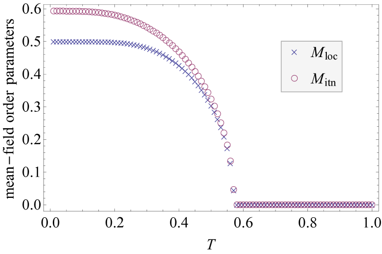
Figure 1: The temperature dependence of the mean-field order parameters $M_{\mathrm{loc}}$ and $M_{\mathrm{itn}}$.

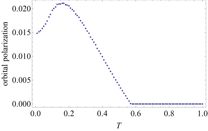
Figure 2: The temperature dependence of the orbital polarization.

IV.2 Dynamic spin susceptibility

For numerical purposes, we use a system size of $N=1000\times 1000$ and $\delta=0.01$ for the ordered state, and $\delta=0.0005$ for the paramagnetic state. A smaller $\delta$ is used for the paramagnetic state so that the energy resolution is appropriate for the lower energy scale involved. A larger $N$ and a smaller $\delta$ do not change our results qualitatively. Figure 3 shows both the imaginary part of the total spin susceptibility for the momentum-space path $\left(0,0\right)$-$\left(\pi,0\right)$-$\left(\pi,\pi\right)$-$\left(0,0\right)$ in both the (a) ordered and (b) paramagnetic states. In the ordered state, the Hund coupling raises the excitation energy at $\left(\pi,\pi\right)$. This effect can be attributed to orbital ordering Lv et al. (2010), which stabilizes order at $\left(\pi,0\right)$ at the expense of competing order at $\left(\pi,\pi\right)$. While the orbital polarization here is an order of magnitude smaller than that found in Ref. Lv et al., 2010, the effect at $\left(\pi,\pi\right)$ remains significant. In addition, the presence of itinerant electrons dampens the excitations around $\left(\pi,\pi\right)$. Figure 4a shows the itinerant components of the bare spin susceptibility $\mbox{Im}\chi_{0}^{+-}$. The regions with strong particle-hole continuum correspond to regions with heavily damped spin-wave excitations. These observations are consistent with the results of INS measurements Diallo et al. (2009); Zhao et al. (2009); Ewings et al. (2011); Harriger et al. (2011, 2012).

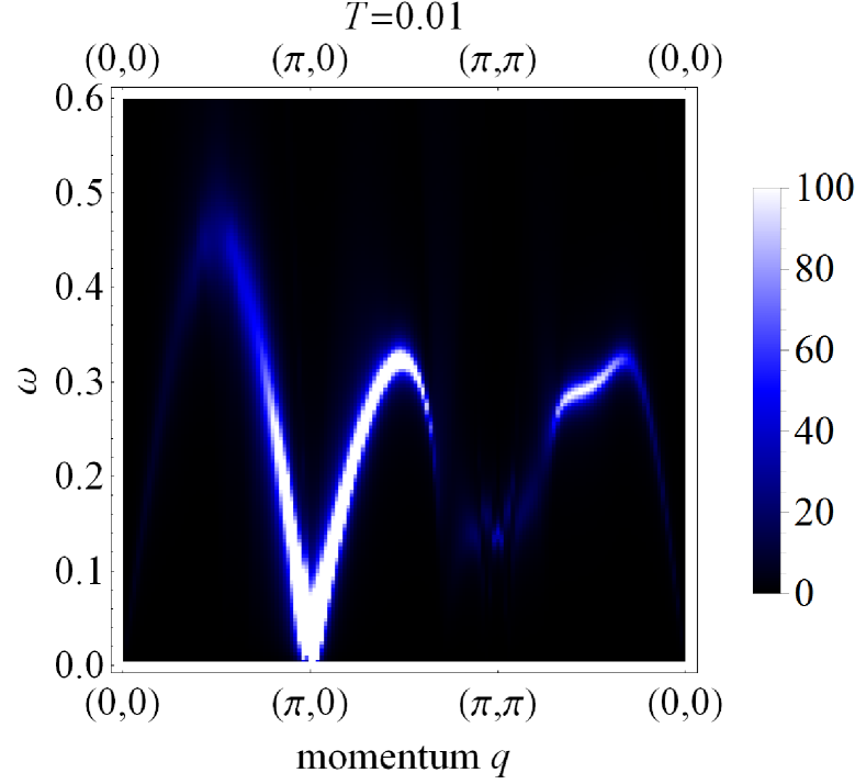
(a)

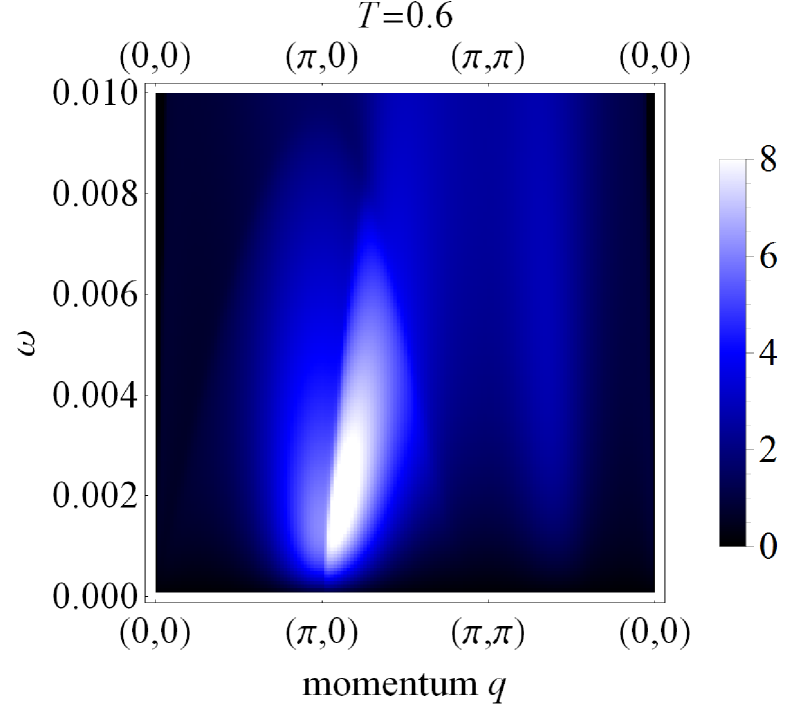
(b)

Figure 3: The total spin susceptibility $\mbox{Im}\bar{\chi}_{\mathrm{tot}}^{+-}$ of the degenerate double-exchange model along the path $\left(0,0\right)$-$\left(\pi,0\right)$-$\left(\pi,\pi\right)$-$\left(0,0\right)$ in the (a) ordered and (b) paramagnetic state. The tight-binding parameters are $t_{1}=-0.5$, $t_{2}=0.65$, and $t_{3}=t_{4}=-0.425$, with an itinerant band filling of $n=2.1$. The superexchange couplings are $J_{1}=0.16$ and $J_{2}=0.6J_{1}$. The Hund coupling is $J_{H}=4$.

Figure 5 shows the temperature dependence of the spin susceptibility along $\left(\pi,\pi\right)$. As the temperature increases, while the excitations around $\left(\pi,\pi\right)$ soften, the Landau damping in the same region increases. Further experiments will be necessary to verify this feature. In the paramagnetic state, the strong spin-wave-like excitation near $\left(\pi,0\right)$ persists, while the particle-hole continuum shown in Figure 4b pushes any collective spin excitations near $\left(\pi,\pi\right)$ to a higher energy. This feature is robust, because a finite particle-hole continuum always exists at the finite wavevector $\left(\pi,\pi\right)$, provided that the single-particle energy spectrum is not fully gapped. Unlike previous theoretical models Goswami et al. (2011); Yu et al. (2012), our results are obtained without breaking $C_{4}$ symmetry. This makes our results applicable to INS measurements even at high temperatures Harriger et al. (2012). This is the key finding of this work.

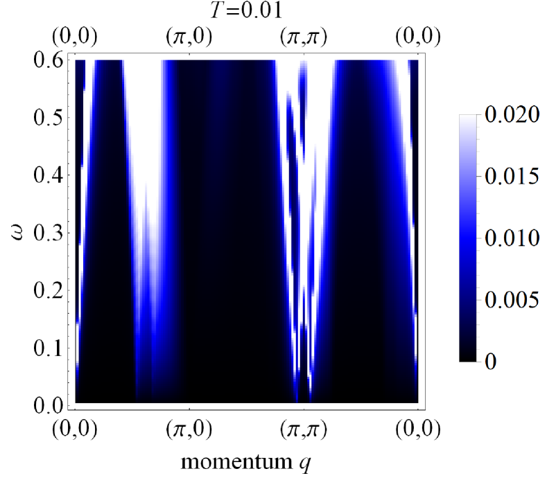
(a)

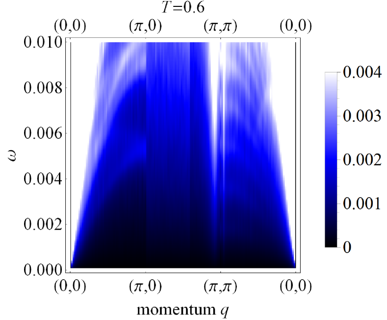
(b)

Figure 4: The itinerant components of the bare susceptibility $\mbox{Im}\chi_{0}^{+-}$ in the (a) ordered and (b) paramagnetic state. The particle-hole continuum dampens the spin-wave excitations.

In our calculation, as the temperature increases in the ordered state, the energy scale of the collective excitations decreases together with the mean-field order parameters. In the paramagnetic state, the energy scale is simply fixed by $\chi_{1},\chi_{2}$. These observations are inconsistent with INS measurements, which show that the energy scale of the collective excitations is independent of temperature. This inconsistency likely arises from the limitations of the mean-field approximation.

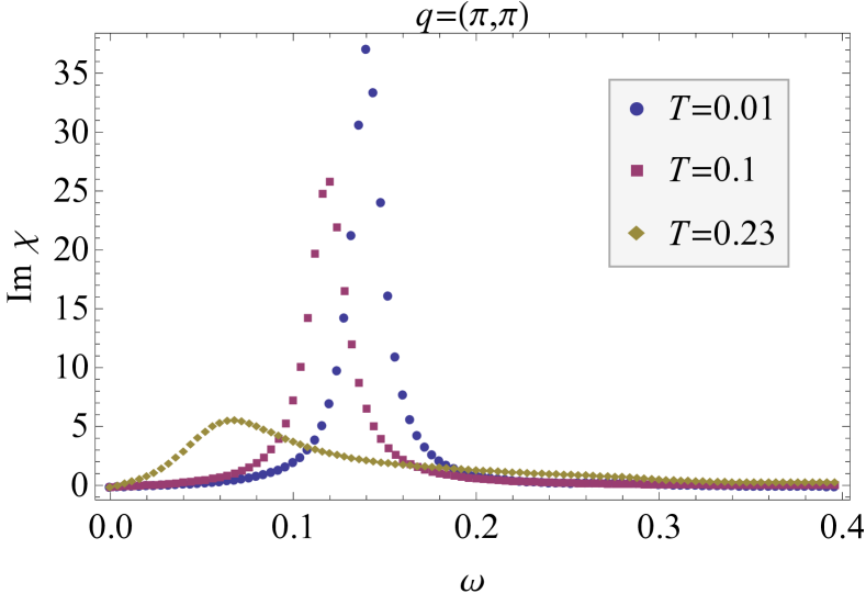
Figure 5: The spin susceptibility along the wavevector $\left(\pi,\pi\right)$ at various temperatures. As temperature increases, excitations around $\left(\pi,\pi\right)$ soften and become more damped.

V Discussion and Conclusion

We also calculated the low-temperature spin susceptibility (not shown) using the tight-binding parameters in Ref. Lv et al., 2010. The excitation energy spectrum is consistent with previous results obtained using the Holstein-Primakoff representation and a linear spin-wave approximation. Compared to the spectrum in Figure 3a, the excitation energy at $\left(\pi,\pi\right)$ has a larger increase due to a stronger orbital order, but the excitations around $\left(\pi,\pi\right)$ are less damped. Therefore, while our results do not qualitatively depend on the choice of parameters, different parameters can be used to produce the quantitative differences between various types of iron pnictides. Furthermore, the $\left(\pi,0\right)$-ordering is robust because the paramagnetic spin susceptibility exhibits a peak at $\left(\pi,0\right)$ despite the itinerant bands having imperfect Fermi surface nesting. This is in contrast with the calculations using only the itinerant model in Ref. Kaneshita and Tohyama, 2010, which show incommensurate peaks.

Our results at high temperatures are consistent with first-principles calculations based on a combination of density functional theory and dynamical mean-field theory Park et al. (2011). This suggests that our model has captured the essential physics of spin excitations in iron pnictides. Since the mechanism for superconductivity is believed to arise from spin fluctuations, it would be important to consider both the local moments and itinerant electrons when studying superconductivity in iron pnictides.

For our choice of parameters, the $d_{xz}$ orbital has a larger occupancy than the $d_{yz}$ orbital. This is opposite the result obtained in Ref. Lv et al., 2010. This difference arises because the opposite sign between the two sets of tight-binding parameters makes occupying the $d_{xz}$ orbital more energetically favorable. This higher occupancy of the $d_{xz}$ orbital agrees with ARPES measurements Yi et al. (2011), which show that the $d_{xz}$ orbital is lower in energy than the $d_{yz}$ orbital in the magnetically ordered state.

To close, we studied the spin excitation spectra of the degenerate double-exchange model. This model consists of local moments represented by a $J_{1}$-$J_{2}$ Heisenberg model, and itinerant electrons from the degenerate $d_{xz}$ and $d_{yz}$ orbitals represented by a tight-binding model. The local moments and itinerant electrons are coupled through a ferromagnetic Hund coupling. Using a fermionic representation of the local moments and a generalized random phase approximation, we obtained a unified framework for the spin excitations in both the ordered and paramagnetic state. The calculated spin susceptibility shows energy spectra and Landau damping consistent with measurements from inelastic neutron scattering experiments over a wide range of temperatures.