BiMAT : a MATLAB^® package to facilitate the analysis and visualization of bipartite networks

Abstract

The statistical analysis of the structure of bipartite ecological networks has increased in importance in recent years. Yet, both algorithms and software packages for the analysis of network structure focus on properties of unipartite networks. In response, we describe BiMAT, an object-oriented MATLAB package for the study of the structure of bipartite ecological networks. BiMAT can analyze the structure of networks, including features such as modularity and nestedness, using a selection of widely-adopted algorithms. BiMAT also includes a variety of null models for evaluating the statistical significance of network properties. BiMAT is capable of performing multi-scale analysis of structure - a potential (and under-examined) feature of many biological networks. Finally, BiMAT relies on the graphics capabilities of MATLAB to enable the visualization of the statistical structure of bipartite networks in either matrix or graph layout representations. BiMAT is available as an open-source package at http://ecotheory.biology.gatech.edu/cflores.

I Background

Biological and social systems involve interactions amongst many components. Such systems are increasingly represented as networks, where nodes denote the interacting objects, and the edges denote the interactions between them newman2010networks . Of course, not all networks are alike. For example, networks are often differentiated based on whether or not individual nodes have the same types of incoming and outgoing links. A network is termed unipartite if any node can potentially connect to any other node, as in metabolic networks jeong2000large , food webs cohen1978food ; dunne2006network , or friendships/contacts in a social network watts1998collective . The interactions between nodes in such networks are often highly structured, i.e. they differ from idealized networks in which the probability of interacting between any two nodes is constant (i.e. the so-called Erdös-Renyi graph erdos1960evolution ). Evaluating the structure of a unipartite network has spurred the development of concepts such as modularity, small-world structure, and hierarchy newman2010networks . Measuring these structures has in turn, led to efficient implementations of algorithms meant to quantify and characterize network structure, primarily that of unipartite networks bastian2009gephi ; shannon2003cytoscape ; hagberg2008exploring ; csardi2006igraph .

In contrast, a network is termed bipartite if nodes represent two distinct types such that interactions can only occur between nodes of different types Chartrand1985 . The canonical example of bipartite networks is that of interactions amongst plant and pollinators, where links represent pollination dunne2006 . Indeed, an abundant literature has emerged on the use of bipartite networks and associated analysis techniques for analysing plant–pollinators systems Bascompte2007 ; Stouffer2011 ; Bascompte2003 ; Bastolla2009 ; Joppa2009 . However, the concept of bipartite networks (and the specific methodology it carries) can be applied in different domains, including the study of antagonistic networks such as host-parasite interactions PoisotBl2011 ; poisot2013structure ; weitz2013phage ; flores2011statistical ; flores2012multi . Bipartite networks, like unipartite networks, are rarely random in their structure, i.e. the probability of any potential link between each pair of nodes of different types is not equal. Studies of both plant-pollinator and host-parasite systems have shown that bipartite networks can be (i) modular, i.e. subsets of nodes often preferentially connect to each other, rather than to other nodes Olesen11122007 ; (ii) nested, i.e. the interaction between nodes can be thought of as subsets of each other flores2011statistical ; Bascompte2003 ; (iii) multi-scale, i.e. the structural properties of the network differ depending on whether the whole or components are considered flores2012multi . As an example, Figure 1 shows Memmot memmott1999structure plant-pollinator network, such that the nested and modular structure only becomes apparent when the appropriate sorting is used. Besides the importance of these metrics to quantity the structure of bipartite empirical data, there is still not a self-contained library or software package for analysing the structure of bipartite networks.

In response, we describe BiMAT , an open-source software for the analysis of bipartite networks. BiMAT is written in MATLAB^® . Although MATLAB^® is proprietary software, its use has increased among ecological research groups due to the fact that producing results and plots is easy and quick. The library includes implementations of the most commonly used algorithms for characterizing the extent to which a bipartite network exhibits modular, nested and multi-scale structure. In addition to measuring the structure of a network, BiMAT also evaluates the statistical significance of this structure given a suite of null models. Finally, BiMAT provides a range of visualization tools for exploring bipartite network structure in either matrix or graph layouts. Here, we first describe the core definitions and methods used in the analysis of bipartite networks. Then, we describe the implementation of BiMAT and its application to a number of examples drawn from virus-host interaction data.

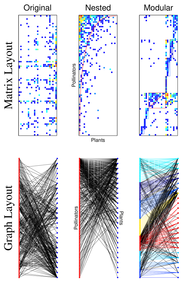
Figure 1: Schematic of an empirical bipartite network (plant-pollinator memmott1999structure ) in matrix and graph layout using the original, nested and modular sorting of plant and pollinator nodes. Color of cells are frequency of visits mapped to $\log$ scale, from small number of visits (darker blue) to large number of visits (dark red). While in the left panels no structure is apparent, the middle and right panels show the opposite. Through visual inspection of the panels, we may infer that the network is nested.

II Methods

II.1 Bipartite ecological network

A bipartite network, $\mathbf{B}$, is a network in which nodes can be divided in two sets $R$ (row nodes) and $C$ (column nodes) such that edges exist only across $R$ and $C$. This type of network can be represented as a bipartite adjacency matrix $\mathbf{B}$ of size $m\times n$, where $m$ is the number of nodes in set $R$ and $n$ is the number of nodes in set $C$. In our implementation, $R$ and $C$ are the node sets that are represented by the rows and columns of the bipartite adjacency matrix in a Bipartite object. Although BiMat takes quantitative matrices as input, all algorithms implemented in BiMAT first threshold these values such that interactions are either present (1) or absent (0). The number of links can be defined as $E=\sum_{ij}B_{ij}$. Finally $k_{i}=\sum_{j}B_{ij}$ and $d_{j}=\sum_{i}B_{ij}$ define the degree (number of interactions) of the two kinds of nodes.

II.2 Algorithms

II.2.1 Modularity

BiMAT use the standard measure of modularity newman2006bmodularity , which for a bipartite network can be defined as (following Barber Barber2007 ):

$$Q_{b}=\frac{1}{E}\sum_{ij}\left(B_{ij}-\frac{k_{i}d_{j}}{E}\right)\delta(g_{i},h_{j}),$$ (1)

where $g_{i}$ and $h_{i}$ are the module indexes of nodes $i$ (that belongs to set $R$) and $j$ (that belongs to set $C$). The idea behind the last equation is to maximize $Q$ by choosing the appropriate indexes for vectors $\mathbf{g}$ and $\mathbf{h}$. Significant debate concerns identifying the optimal set of modules in the case of bipartite networks fortunato2010community ; sawardecker2009comparison . In order to provide multiple options, BiMAT uses three different algorithms to maximize Equation 1: Adaptive BRIM Barber2007 , LP-BRIM liuxin and the leading eigenvector method newman2006bmodularity .

• AdaptiveBRIM: The standard BRIM (for Bipartite Recursively Induced Modules) algorithm works in the matricial notation version of Equation 1 given by:

  $$Q_{b}=\frac{1}{E}\operatorname{Tr}\mathbf{R}^{T}\mathbf{\tilde{B}}\mathbf{T},$$ (2)

  where $\tilde{B}_{ij}=B_{ij}-\frac{k_{i}d_{j}}{E}$ is often called the modularity matrix. Further, we replaced the delta function and vectors $\mathbf{g}$ and $\mathbf{h}$ by the $m\times c$ index matrix ${\bf R}=\left[{\bf r}_{1}|{\bf r}_{2}|...|{\bf r}_{m}\right]^{T}$ and the $n\times c$ index matrix ${\bf T}=\left[{\bf t}_{1}|{\bf t}_{2}|...|{\bf t}_{n}\right]^{T}$, for row and column nodes, respectively, with $c$ denoting the number of modules Barber2007 . Notice that nodes cannot be classified into more than one module. Hence, vectors ${\bf r}_{i}$ and ${\bf t}_{i}$ consist of a single one (corresponding to the chosen module) with all the other entries being zero. For example, $r_{ik}=1$ if the $i$-th row node belongs to the $k$-th module with $r_{ij}=0$ for all $j\neq k$. Using the last expression, the standard BRIM algorithm computes the optimal modularity by inducing the division of one set of nodes (say vector ${\bf T}$) from the division in the other set of nodes (say vector ${\bf R}$). At each step, BRIM assigns nodes of one type to modules in order to maximize the modularity. BRIM iterates this process until a local maximum is reached. However, the choice of a predefined number $c$ of modules limits the efficacy of the algorithm. Hence, we use an adaptive heuristic Barber2007 to identify the optimal set of modules (and associated modularity $Q$). This heuristic assumes that there is a smooth relationship between the number of modules $c$ and the modularity $Q_{b}(c)$. For continuous and smooth landscapes, a simple bisection method ensures that we will find the optimal value of $c=c^{\star}$ corresponding to maximum $Q_{b}$. Starting at $c=1$ (and modularity $Q_{b}(1)=0$ because all nodes belong to the same module) the adaptive BRIM searches for optimal $c$ by repeatedly doubling the number of modules while modularity increases, $Q_{b}(2c)>Q_{b}(c)$. At some point, the search crosses a maximum in the modularity landscape, i.e. $Q_{b}(2c)<Q_{b}(c)$, and we interpolate the number of modules $c^{\star}$ to some intermediate value in the interval $(c/2,2c)$.

• LP&BRIM: The algorithm is a combination between the BRIM and LP (Label Propagation) algorithms. The heuristic of this algorithm consists in searching for the best module configuration by first using the LP algorithm. This algorithm initially assigns each node to a different module (label). At each interaction the module of each node is reassigned to the module to which the majority of its neighbours belong to. The order of node reassignment is random and ties are broken randomly. The algorithm continues until convergence is achieved. The standard BRIM algorithm is used at the end to refine the results.

• LeadingEigenvector: This algorithm works with the unipartite adjacency matrix $\mathbf{A}$ of size $m+n\times m+n$ instead of the bipartite adjacency matrix $\mathbf{B}$. The modularity using this notation can be defined for two modules in matrix notation as newman2006bmodularity :

  $$Q=\frac{1}{4E}\mathbf{s}^{T}\mathbf{\tilde{A}}s,$$ (3)

  where $\tilde{A}_{ij}=A_{ij}-\frac{k_{i}k_{j}}{2E}$ is the modularity matrix expressed using the unipartite adjacency matrix with no distinction for degrees or rows and columns. Further, for a particular division of the network into two modules, $s_{i}=1$ if node $i$ belongs to module 1 and $s_{i}=-1$ if it belongs to module 2. The idea of this algorithm is that we can decompose the previous equation in a linear combination of the normalized eigenvectors $u_{i}$ of $\mathbf{\tilde{A}}$ so that $\mathbf{s}=\sum a_{i}\mathbf{u}_{i}$ with $a_{i}=\mathbf{u}_{i}^{T}\cdot\mathbf{s}$:

  $$Q=\frac{1}{4E}\sum a_{i}\mathbf{u}_{i}^{T}\mathbf{\tilde{A}}\sum a_{j}\mathbf{u}_{j}=\frac{1}{4E}\sum(\mathbf{u}_{i}^{T}\cdot\mathbf{s})^{2}\alpha_{i},$$ (4)

  where $\alpha_{i}$ is the eigenvalue of $\mathbf{\tilde{A}}$ corresponding to eigenvector $\mathbf{u}_{i}$. The leading eigenvector name comes from the fact that in order to maximize the last equation what we can do is to focus only in the sum term with the maximum eigenvalue $\mathbf{\alpha}_{max}$ which corresponds the leading eigenvector $\mathbf{u}_{max}$. This term can be maximized by trying to maximize $\mathbf{u}_{max}\cdot\mathbf{s}$. Because $s_{i}$ can only have the values $\pm 1$, this can be solved by assigning $s_{i}=1$ and $s_{i}=-1$ when $\mathbf{u}_{max_{i}}>0$ and $\mathbf{u}_{max_{i}}\leq 0$, respectively, which completes the core of the leading eigenvector algorithm. After performing the first iteration of the last process we will have a subdivision of just two modules. Newman newman2006bmodularity then explain that this process can be applied recursively in each of the subdivisions. However, instead of isolating each subdivision of each other, we apply this heuristic in the expression $\Delta Q$ which defines the change of modularity that a new subdivision in an specific module will give us. The subdivision is only accepted if $\Delta Q>0$. For mode details about $\Delta Q$ we recommend to read newman2006bmodularity . Finally, it is worth to mention that in BiMAT by default each subdivision is refined using the Kernighan–Lin algorithm kernighan1970efficient too. The essence of this algorithm is swapping nodes between the two modules such that at each step the node that gives the biggest increase in $Q$ or the smallest decrease (if increase is not possible) is swapped. In a complete iteration all nodes are swapped with the constraint that a node is swapped only once. The intermediate state during the iteration that has the biggest $Q$ is selected as the new configuration and the process repeats using this new configuration until no improvement is possible.

In addition to optimize the standard modularity $Q_{b}$ BiMAT also evaluates (after optimizing $Q_{b}$) an a posteriori measure of modularity $Q_{r}$ introduced in poisot2013posteriori and defined as:

$$Q_{r}=2\times\frac{W}{E}-1$$ (5)

where $W=\sum_{ij}B_{ij}\delta(g_{i},h_{j})$ is the number of edges that are inside modules. Alternatively, $Q_{r}\equiv\frac{W-T}{W+T}$ where $T$ is the number of edges that are between modules. In other words, this quantity maps the relative difference of edges that are within modules to those between modules on a scale from 1 (all edges are within modules) to $-1$ (all edges are between modules). This measure allows to compare the output of different algorithms.

II.2.2 Nestedness

Nestedness is a term used to describe the extent to which interactions form ordered subsets of each other. Multiple indices are available to quantify nestedness (see ulrich2009consumer for details about many of these measures). Two of the most commonly used methods are: NTC (Nestedness Temperature Calculator) Atmar1993 ; Rodriguez-Girones2006 and NODF (for Nestedness metric based on Overlap and Decreasing Fill) almeida2008consistent . Both of these are implemented in BiMAT and are summarized below:

• NestednessNTC (NTC): A ‘temperature’, $T$, of the interaction matrix is estimated by resorting rows and columns such that the largest quantity of interactions falls above the isocline (a curve that will divide the interaction from the non-interaction zone of a perfectly nested matrix of the same size and connectance). In doing so, the value of $T$ quantifies the extent to which interactions only take place in the upper left ($T\approx 0$), or are equally distributed between the upper left and the lower right ($T\approx 100$). Perfectly nested interaction matrices can be resorted to lie exclusively in the upper left portion and hence have a temperature of 0. The value of temperature depends on the size, connectance and structure of the network. Because the temperature value quantifies departures from perfect nestedness, we define the nestedness, $N_{NTC}$, of a matrix to range from 0 to 1, $N_{NTC}=(100-T)/100$, such that $N_{NTC}=1$ when $T=0$ (perfect nestedness) and $N_{NTC}=0$ when $T=100$ (checkerboard).

• NestednessNODF: NODF is independent of row and column order. This algorithm measures the nestedness across rows by assigning a value $M_{ij}^{\text{rows}}$ to each pair $i$, $j$ of rows in the interaction matrixalmeida2008consistent :

  $$M_{ij}^{\text{rows}}=\begin{cases}0&\text{if $k_{i}=k_{j}$}\\ n_{ij}/\min(k_{i},k_{j})&\text{otherwise}\end{cases}$$ (6)

  where $n_{ij}$ is the number of common interactions between them. A similar term is used for the column contributions, such that the total nestedness is defined as:

  $$N_{NODF}=\frac{\sum_{i<j}M_{ij}^{\text{rows}}+\sum_{i<j}M_{ij}^{\text{columns}}}{m(m-1)/2+n(n-1)/2}.$$ (7)

  However, BiMAT redefined Equation 6 (and its column version), such that the last equation can be more easily vectorized:

  $$M_{ij}^{\text{rows}}=\frac{(\mathbf{r}_{i}\cdot\mathbf{r}_{j})\delta(k_{i},k_{j})}{\min(k_{i},k_{j})},$$ (8)

  where $\mathbf{r_{i}}$ is a vector that represents the row $i$ of the bipartite adjacency matrix. Equation 7 can be rewritten in terms of adjacency matrix multiplications (see code for details). This new vectorized version of calculating the $N_{NODF}$ value outperforms the naive one (using loops) by a factor over 50 in most of the matrices that we tested.

Note that a new eigenvalue-eigenvector approach to evaluating nestedness has recently been introduced staniczenko2013ghost , which will be introduced in a future BiMAT release.

II.3 Statistics

II.3.1 Null Models

We propose four null models to test the significance of measured nestedness and modularity (see Bascompte2003 ; ulrich2007null ; flores2011statistical ; poisot2013structure for more details). These null models generate random networks through a Bernoulli process, where the probability of interactions are determined following different rules. Define $k_{i}$ as the degree of a node $i$ of the column class and $d_{j}$ as the degree of a node $j$ of the row class. Then, the probability that two nodes (of distinct classes) interact, $P_{ij}$ is:

EQUIPROBABLE

, $P_{ij}=E/(mn)$ – the connectance of the network is respected, but not the number of interactions in which each node is involved.

AVERAGE

, $P_{ij}=(k_{i}/n+d_{j}/m)/2$ – the connectance, and the expected number of interactions in which each node is involved, are respected

COLUMNS

, $P_{ij}=k_{i}/n$ – the connectance, and the expected number of interactions of row nodes, are respected

ROWS

, $P_{ij}=d_{j}/m$ – the connectance, and the expected number of interactions of column nodes, are respected

By default, BiMAT generate networks that can have disconnected nodes (i.e. nodes with no edges to any other nodes in the network). However the user can impose a constraint that all nodes must be connected to at least one other node (if possible) in the null model generating process. Note that BiMAT does not include some of the most constrained null models, e.g., random networks that respect not only the expectation of connectance and degree but also the exact degree sequences as the original network staniczenko2013ghost ,

II.3.2 Statistic Values

Once an ensemble of random networks is specified, BiMAT will return the following values:

• value: value to be tested (e.g. nestedness or modularity).

• random_values: the values of all random replicates.

• replicates: number of replicates used during testing.

• mean: mean of the replicate values.

• std: standard deviation of the replicate values (note that distributions of network values are not necessarily well described by a normal distribution).

• zscore: The $z$-score of value assuming that the replicate values represent the entire population.

• percentile: The percentage of replicate values that are smaller than value.

II.3.3 Extended statistics

As described above, BiMAT enables the evaluation of the statistical significance of modularity and nestedness. Additional statistical evaluation is possible, including the capability to conduct a meta-analysis and a multi-scale analysis.

Meta analysis

: BiMAT can simultaneously analyse the network structure of a set of related bipartite networks (e.g. plant-pollinator networks or virus-host interaction networks). In which case, the distribution of network properties of the set of networks can be analysed (see example I in the Examples section for more details).

Multi-scale analysis

: Individual modules need not always be homogeneous. Hence, BiMAT offers functionality to evaluate whether or not the network has different structures at different scales, e.g., the overall network may be modular, but individual modules may be nested (see example II in the Examples section for more details).

III The BiMAT package

BiMAT is a open-source package (see Figure 2) written in MATLAB^® . It is primarily designed for the analysis and visualization of bipartite ecological networks, thought it may be used for any type of bipartite networks. The package aims to consolidate some of the most popular algorithms and metrics for the analysis of bipartite ecological networks in the same software environment. Specifically, the core features examined are bipartite modularity Barber2007 and nestedness Atmar1993 ; almeida2008consistent . Further, BiMAT include the necessary tools for analysing the statistical significance of these values, together with tools for visualizing bipartite networks in such a way that these properties becomes apparent to the user. BiMAT utilizes an object-oriented framework which enables users to extend the package.

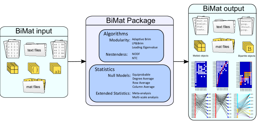
Figure 2: BiMAT Workflow. The figure shows the main scheme of the BiMAT package. BiMAT can take matlab objects or text files as main input. The input is analysed mainly around modularity and nestedness using a variety of null models. The user may also perform an additional multi-scale analysis on the data, or if he have more than one matrix to perform a meta-analysis in the entire data. Finally, the user can observe the results via matlab objects, text files and plots.

III.1 Usability

Users are expected to be familiar with the MATLAB^® environment. However, BiMAT has been designed so that even MATLAB^® beginners or those with very limited expertise can easily carry out a comprehensive analysis and visualization of their data, in many cases with a single command. Despite an emphasis on simplicity, BiMAT still retains all of the functionality and flexibility provided by the MATLAB^® environment (e.g., all the results are returned to the current session workspace, the results can be stored in MATLAB^® files, and the class properties can be used for MATLAB^® plotting). A complete start guide is distributed with the library.

III.2 Comparison with other software

Current and popular available tools for the analysis of complex networks include implementations that are predominantly: (i) visually oriented (e.g. Gephi bastian2009gephi , Cytoscape shannon2003cytoscape ) or (ii) library-package oriented (e.g. networkx hagberg2008exploring , iGraph csardi2006igraph ). Unfortunately, these tools have a strong focus on the analysis of unipartite networks, i.e. bipartite networks are treated as a special case of a unipartite network. As a consequence, algorithms for the analysis of unipartite networks, when applied to bipartite networks, are not intended to be optimal, neither where designed to the study of ecological bipartite networks. In contrast, specialized tools for the analysis of bipartite ecological networks are available but they are very specific (e.g. ANINHADO guimaraes2006improving , WINE galeano2009weighted , and recently FALCON falconNest focus only in nestedness analysis).

However, the authors acknowledge the existence of bipartite bipartiteR , a software library written in R. Thought this library initially included only nestedness analysis regarding internal network structure, they just recently aggregated modularity analysis too dormann2014method . BiMAT does not intent to replace this library but to complemented by bringing similar tools to the MATLAB^® ecology community. Further, BiMAT also includes tools for the analysis of many related networks (meta analysis) and for the analysis of different levels of the same network (multi-scale analysis), which will facilitate the statistical analysis of bipartite ecological networks. Whereas bipartite strives for exhaustivity, BiMAT focuses on implementing a well-documented core of statistical procedures in an optimized way.

In summary, BiMAT provides a broad selection of tools required for the analysis and visualization of bipartite ecological networks. As such, BiMAT is aimed towards empiricists seeking to apply a network perspective to their data, and is particularly suited to exploratory analyses of data derived from ecological, evolutionary, and environmental datasets. Table 1 show the current tools of current libraries.

Table 1: Bipartite Ecological libraries

Software	Language	Open Source	Visualization	Nestedness	Modularity	Meta-analysis	Multi-scale analysis
ANINHADO guimaraes2006improving	Executable	✗	✗	✓	✗	✓	✗
WINE galeano2009weighted	MATLAB® /R/C++	✓	✓	✓	✗	✗	✗
FALCON falconNest	MATLAB® /R	✓	✓	✓	✗	✗	✗
bipartite bipartiteR	R	✓	✓	✓	✓	✗	✗
BiMAT	MATLAB®	✓	✓	✓	✓	✓	✓

III.3 Installation

BiMAT stable version can be downloaded directly from the main author webpage: http://ecotheory.biology.gatech.edu/cflores. Last updated version can be downloaded from https://github.com/cesar7f/BiMat.

III.4 License and bug tracking

The software is distributed using FreeBSD license, which basically means that the user can redistribute it, with or without modification for any kind of purpose as long as its copyright notices and the licence’s disclaimers of warranty are maintained. Though the license do not force users to do so, we encourage them to cite this paper if the use of BiMAT library leads to any kind of scientific publication.

Users can report bugs directly in the github repository (see URL above), provided they have a github account.

III.5 Configuration

The BiMAT directory should be added to the MATLAB^® paths. At this point, BiMAT can be executed without any additional configuration. The default parameters for algorithms implemented in the BiMAT package are available in file main/Options.m. Additional details are available in the Start Guide, including as part of the BiMAT package (and released here as Supplementary File X).

III.6 Objected-Oriented Programming Scheme

BiMAT has been coded using the Objected-Oriented Programming (OOP) paradigm. Note that understanding of OOP is not required for use of BiMAT . Nonetheless, the use of OOP is meant facilitate maintainability and extensibility of the codebase. Access to BiMAT functions is granted (with the exception of some static classes) using instances of the class that implements the functions.

The main package class is the Bipartite class, whose only function is to work as a common interface to all of the available statistical, algorithmic, plotting, and input/output classes. Because of this OOP design pattern, most of the MATLAB^® functionality will be granted using the following syntax:

bip.class_instance_in_bip.method_name(arguments)

where bip is a bipartite instance created by the user, class_instance_in_bip is a property of the bipartite class which represents an instance of the class which has access to the method method_name. The method that is called will frequently have direct read and writeable access to other properties inside bip. Table 2 shows the main calls from the Bipartite object, assuming that the user call its bipartite instance bip.

Note that the OOP capabilities of MATLAB^® are not as extensive as those of OOP focus languages (e.g. python, Java, C++). As such, certain behaviours have been emulated in BiMAT , e.g. static classes were emulated using private constructors. However, in contrast to other languages that enable OOP, MATLAB^® enables users to store created instances as MATLAB^® objects in files. This ensures that users can save, and subsequently load, the results of partial analysis.

Table 2: Some useful calls using the OOP approach

Call	Class	Description
bip.community.Detect()	BipartiteModularity	Calculate Modularity
bip.nestedness.Detect()	Nestedness	Calculate nestedness
bip.statistics.DoCompleteAnalysis()	StatisticalTest	Executes the required commands in order to have
		a complete analysis of nestedness and modularity
bip.statistics.DoNulls()	StatisticalTest	Create the null model matrices
bip.statistics.TestCommunityStructure()	StatisticalTest	Perform the statistical test for modularity values
bip.statistics.TestNestedness()	StatisticalTest	Perform the statistical test of nestedness value
bip.internal_statistics.TestDiversityRows()	InternalStatistics	Perform diversity analysis across rows
bip.internal_statistics.TestDiversityColumns()	InternalStatistics	Perform diversity analysis across columns
bip.internal_statistics.TestInternalModules()	InternalStatistics	Perform an statistical test
		for modularity and nestedness inside modules
bip.plotter.PlotMatrix()	PlotWebs	Plot a matrix layout of the original data
bip.plotter.PlotModularMatrix()	PlotWebs	Plot a matrix layout of the modular sorted data
bip.plotter.PlotNestedMatrix()	PlotWebs	Plot a matrix layout of the nested sorted data
bip.plotter.PlotGraph()	PlotWebs	Plot a graph layout of the original data
bip.plotter.PlotModularGraph()	PlotWebs	Plot a graph layout of the modular sorted data
bip.plotter.PlotNestedGraph()	PlotWebs	Plot a graph layout of the nested sorted data

III.7 Input/Output

The class bipartite is the main class of the package. Hence, a user will usually need to work with at least one instance of this class. An instance of this class requires a boolean MATLAB^® matrix object, representing the bipartite adjacency network. Alternatively, a integer matrix can be provided e.g., when the values represent categorical levels of interactions, and these categorical levels can be included in the visualization tools. Optional arguments that can be passed are the row and column node labels and classification classes. These arguments need to be passed directly to the properties of the Bipartite object. In practice, an object of the class Bipartite can be created as follows:

bip = Bipartite(matrix);
bip.row_labels = rowLabels;
bip.col_labels = colLabels;
bip.row_class = rowClasses;
bip.col_class = colClasses;

in which the variables matrix, rowLabels, colLabels, rowClasses and colClasses are previously defined variables. Network information, including adjacency matrix and node labels, can be read directory from data files using the static class Reading:

• bip = Reader.READ_BIPARTITE_MATRIX(filename): The file should be in the following format:

  Ψ1 0 0 2 0 0 0
  Ψ1 2 0 0 0 2 1
  Ψ1 1 0 0 1 2 1
  Ψ1 2 3 0 0 1 1
  Ψ2 1 1 1 0 0 0
  Ψ
  

  Each row in the file represents a different outgoing set of interaction from a node (in set A) to a different set of nodes (in set B) in the columns. All values different from 0 are counted as interactions, such that evaluation of network structure utilizes Boolean information whereas visualization can leverage the non-negative strengths of interactions:

• bip = Reader.READ_ADJACENCY_LIST(filename): The file should be an ordered list of triples:

  Ψrow_label_1 1 col_label_1
  Ψrow_label_1 1 col_label_2
  Ψrow_label_1 2 col_label_3
  Ψrow_label_3 1 col_label_2ΨΨΨ
  Ψrow_label_3 3 col_label_1
  Ψrow_label_2 3 col_label_2Ψ
  Ψ
  

  such that the first and third columns represent nodes from sets A and B, respectively, and (an optional) second column denoting the strength of interactions.

III.8 Functional alternative

Static functions can be used as an alternative to interacting with the BiMAT package in an OOP framework. For example, the network can be visualized in a graph or matrix layout as follows:

PlotWebs.PLOT_MATRIX(matrix);
PlotWebs.PLOT_GRAPH(matrix);

instead of:

bp = Bipartite(matrix);
bp.plotter.PlotMatrix();
bp.plotter.PlotGraph();

Table 3 shows some of the most important static functions that provide access to part of the BiMAT functionality.

Table 3: Useful calls in the functional approach

Call	Description
BipartiteModularity.ADAPTIVE_BRIM(matrix)	Calculate the modularity values using the Adaptive BRIM algorithm
BipartiteModularity.LP_BRIM(matrix)	Calculate the modularity values using the LP&BRIM algorithm
BipartiteModularity.LEADING_EIGENVECTOR(matrix)	Calculate the modularity values using the Leading Eigenvector algorithm
Nestedness.NODF(matrix)	Calculate the NODF values
Nestedness.NTC(matrix)	Calculate the NTC values
PlotWebs.PLOT_MATRIX(matrix)	Plot the data in matrix layout
PlotWebs.PLOT_NESTED_MATRIX(matrix)	Plot the nested sorted data in matrix layout
PlotWebs.PLOT_MODULAR_MATRIX(matrix)	Plot the modular sorted data in matrix layout
PlotWebs.PLOT_GRAPH(matrix)	Plot the data in graph layout
PlotWebs.PLOT_NESTED_GRAPH(matrix)	Plot the graph sorted data in matrix layout
PlotWebs.PLOT_MODULAR_GRAPH(matrix)	Plot the graph sorted data in matrix layout
Printer.PRINT_GENERAL_PROPERTIES(matrix)	Print to screen the general properties of the network
Printer.PRINT_STRUCTURE_VALUES(matrix)	Print the modularity and nestedness values of the network

III.9 Plotting

The class PlotWebs provides the required functions to visualize a bipartite network in a matrix or graph layout. Visualization can utilize (i) the original sorted version of the data, (ii) the nested sorted version of the data, or and (iii) the modular sorted version of the data. BiMAT represents the interaction data with colored cells when a matrix layout is used. Rows and columns denote members of the the two sets and cells denote interaction strength. The format of the matrix is specified by modifying the PlotWebs class properties before calling the plotting functions. Further, the format of the matrix will depend on what kind of sorting is used. For example, the modular sorting plot can color the cells according to the module to which they belong to or the type of interaction. Some features are restricted to particular sortings, e.g., plotting an isocline (see Methods) is available only in the nested and modular sorting. Alternatively, the PlotWebs can plot the data in a graph layout in which members of the two sets A and B are depicted using a stacked set of circles to the left and right, respectively. Lines are draw between sets that interact. As for matrices, many of the properties of PlotWebs can be used to specify the format of the plot (see documentation).

In addition to this main class, BiMAT has an additional plot class called MetaStatisticsPlotter that is used for plotting meta-analysis results (analysis of many networks). This class can plot statistical results of the structural quantities of the algorithms, together with visual graph or matrix layout representations of the networks (see Examples section).

III.10 Performance

The BiMAT packages leverages optimization tools of MATLAB^® . For example, algorithms implemented in BiMAT were vectorized to improve performance. In addition, a version of BiMAT that uses the MATLAB^® Parallel Computing Toolbox can be requested to the corresponding author.

IV Examples

We present here two examples to illustrate the potential use of BiMAT for visualization and analysis of bipartite complex networks: (i) a meta-analysis of 38 different phage-bacteria interaction networks; (ii) a multi-scale analysis of the largest phage-bacteria interaction network. Scripts and data for these examples are included in the BiMAT release and additional documentation is included in the start guide.

IV.1 Example I: Meta-analysis

The study of virus-host interactions includes examination of whom infects whom. Exhaustive assays of cross-infection of a set of phages (viruses that infect and kill bacteria) and a set of bacteria are generally reported as a bipartite cross-infection matrix. These matrices can be standardized such that rows and columns represent bacteria and phages, respectively. The cell enrties in these matrices represent the level of infection between phages and bacteria. In a previous study, Flores et al flores2011statistical re-examined 38 such networks extracted from the published literature between 1950 and 2011. In doing so, the authors found that phage-bacteria infection networks (as published) tend to be nested and not modular. BiMAT can reproduce these results using the MetaStatistics module.

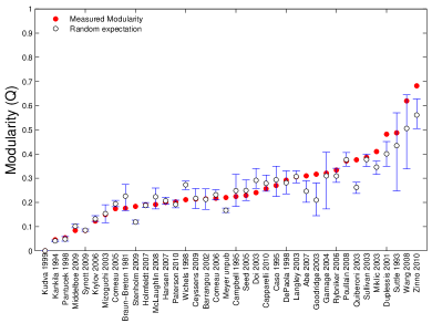
(a) Modularity statistics

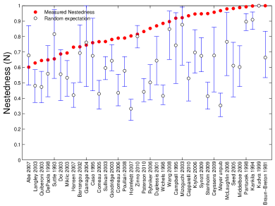
(b) Nestedness (NTC) statistics

Figure 3: Visual representation of the statistical tests in the set of matrices. Red circles represent the value of the analyzed networks. White circles represent the mean of the null model, while the error bars represent the networks that falls inside a two-tailed version of the random null model values. The margin of the error bars are (p-value,1-p-value), where p-value can is an optional argument of the plot functions.

First, the user should begin by creating an instance of the MetaStatistics class. This class takes, as input, a cell array matrices containing either a set of MATLAB^® matrices or a set of Bipartite objects. An automatic meta-analysis, using default parameters, can be performed by the commands:

mstat = MetaStatistics(matrices);
mstat.names = matrix_names %Labels for networks
%chosing the algorithms:
mstat.modularity_algorithm = @AdaptiveBrim
mstat.nestedness_algorithm = @NestednessNTC
mstat.DoMetaAnalyisis();

Results of the meta-analysis are stored in the object gstat, for subsequent examination. The meta-analysis class (MetaStatistics.m) also has additional plot functions. e.g., to compare network structures against a null model values:

mstat.plotter.PlotModularValues(0.05);
mstat.plotter.PlotNestednessValues(0.05);

where the argument represent the p-value threshold in determining the variation about the network statistics generated from the ensemble (lower values denote wider variation). The output for the modular and NTC values can be observed in Figure 3. As is apparent, the majority of studies have modularity below that of the networks in the random ensemble. In contrast, the majority of studies have nestedness significantly above that of the networks in the random ensemble.

In addition, it is possible to plot all the matrices at once using any of the next functions:

%Grid of 5 x 8
mstat.plotter.PlotMatrices(5,8);
mstat.plotter.PlotNestedMatrices(5,8,0.05);
mstat.plotter.PlotModularMatrices(5,8,0.05);

where the first and second arguments are the number the matrices along horizontal and vertical axis of the plot. If the statistical test have been already performed, red and blue labels are used for indicate the statistical significance of the corresponding structure (red for significance, and blue for anti-significance), where the third argument (optional) is used to assess a critical $p$-value the significance. Figure 4 shows the plot for the case of modularity.

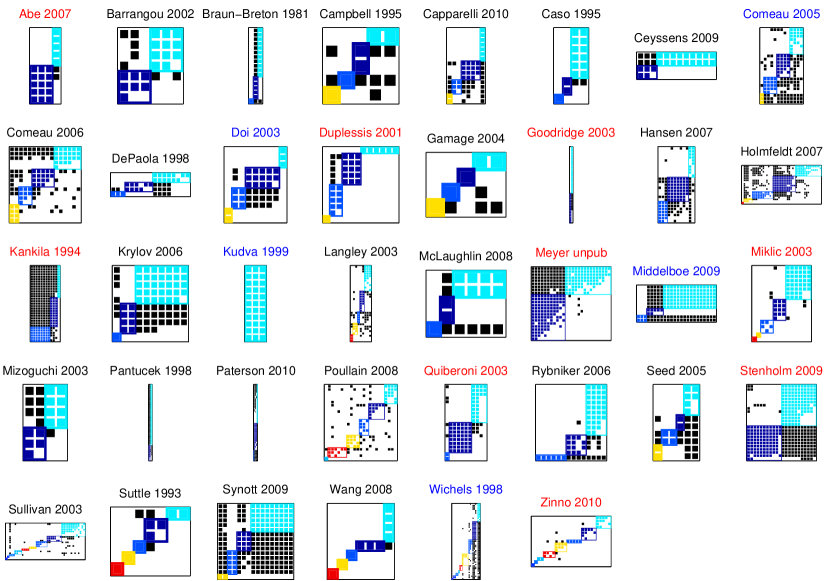
Figure 4: The meta-set collected on Flores et al flores2011statistical plotted using the modularity algorithm of the BiMAT library. Red and blue labels represent significant modularity ($p\geq 0.975$) and anti-modularity ($p\leq 0.275$), respectively. For bibliographic information about these matrices see flores2011statistical .

IV.2 Example II: Multi-scale analysis

Moebus and Nattkemper moebus1981bacteriophage published the largest phage-bacteria infection network. The individual phage and bacteria were extracted from different locations across the Atlantic Ocean. In a previous study we developed a multi-scale analysis of network structure in this datasetflores2012multi . Here, we demonstrate how such a multi-scale analysis can be automated. The first objective is to analyze the global-scale structure of a bipartite network, i.e. to quantify if the overall network has significantly elevated or diminished modularity and/or nestedness. Assuming that our matrix is called moebus.weight_matrix left panel of Figure 5 shows a visual representation of this data in matrix layout after typing:

bp = Bipartite(moebus.weight_matrix);
bp.community.Detect();
bp.plotter.font_size = 2.0;
figure(1);
bp.plotter.PlotModularMatrix();

It becomes apparent that the network is modular. However, what is really important to observe is that internal nodes seems to have nested structure (triangular pattern with most of the links above the isocline). Hence, the Moebus network may have multi-scale structure properties. We will confirm that this is the case for nestedness using the $N_{NTC}$ values. In order to perform this test BiMAT make use of the InternalStatistics class in order to get the statistics of those modules by isolating them and treating them as independent networks:

%We are interested in only the first 15 modules
%from the most righ-top one.
bp.internal_statistics.idx_to_focus_on = 1:15;
%Perform a default internal analysis
bp.internal_statistics.TestInternalModules();
figure(2);
bp.internal_statistics.meta_statistics...
             .plotter.PlotNestednessValues();
figure(3);
bp.internal_statistics.meta_statistics...
             .plotter.PlotNestedMatrices();

where the last two plots are the ones on the right panels of Figure 5. The smart reader may already notice that meta_statistics property is in fact an instance of the class MetaStatistics, which translates to be able to use any of the methods inside MetaStatistics (including its property plotter) in the internal modules.

Finally, another multi-scale analysis that BiMAT can perform is to quantify if a relation exist between node classification and module distribution. If the extreme case, if this relation exist nodes inside the same module will share the same classification. If the such relationship does not exist, modules will have nodes with random classification. In order words, the relationship depends in how random is the node classification inside the each module. In order to perform this analysis BiMAT make use of both Shannon’s and Simpon’s indexes. And, for evaluating the significance we use a null model in which we randomly swap all node classifications. We will give here a simple example about how to print the significance of Simpson’s index for the case of phage (column) nodes. In order to do so, we will use geographical location extraction as classification identifier of each node:

% We want to use geographical location
% as classification
bp.col_class = moebus.phage_stations;
% Perform the analysis
bp.internal_statistics.TestDiversityColumns();
% Print results
bp.printer.PrintColumnModuleDiversity();

The user must be able to visualize an output similar to:

Diversity index:    Ψ  Diversity.SIMPSON_INDEX
Random permutations:Ψ                      100
Module,index value,  zscore,percent
     1,    0.94805, -1.3848,      6
     2,    0.91738, -5.0054,      0
     3,    0.95238,-0.42625,     11
     4,    0.81667,-13.1025,      0
     5,          1, 0.36742,     12
     6,    0.85714, -2.5808,      0
     7,    0.66667, -2.4661,      0
     8,    0.33333,-13.5825,      0
     9,    0.90909, -2.0933,      3
    10,        0.9, -1.1203,      2
    11,        0.5, -6.6773,      0
    12,    0.88889, -2.6493,      1
    13,        0.6, -7.0097,      0
    14,        0.6, -8.0336,      0
    15,    0.83333, -1.3318,      3

If we want to use the percentile as statistical test (using one-tail) and $p$-value=0.5 we have that 12 modules are not as diverse as the random expectation. Hence, these modules contain phages that come from similar geographical stations, which translate to potentially have a relationship between the geographical location and module formation for the phages case.

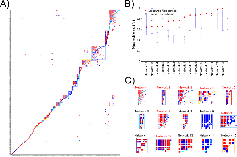
Figure 5: Standard plots that can be extracted using the multi-scale analysis capabilities of BiMAT . Here, we focus in the internal nested structure using $N_{NTC}$ values, but we can also perform an internal study using $Q_{b}$ and $N_{NODF}$ values. A) The standard output using the modular matrix layout gives us a hint about the potential multi-scale structure. B) Here we focus on the study of $N_{NTC}$ values with respect to random expectation. Error bars cover 95 % of the random replicate values. C) A more closer visual inspection on the analyzed matrices. Read labels indicate statistical significance of $N_{NTC}$ values.

V Future Work

We have developed BiMAT – an extensible MATLAB^® library for the analysis of bipartite networks. BiMAT implements standard algorithms for the quantification of network structure, including multiple tools to facilitate the analysis of the significance of network structure at the whole network scale, across networks and within networks. The focus on two network features, modularity and nestedness, reflects the importance both have in analyses of bipartite network structure in ecological datasets. However, these are not the only potential features of a bipartite network nor are they necessarily independent.

Indeed, it has been suggested that modularity and nestedness can be strongly correlated fortuna2010nestedness . Such correlations may, on the one hand, lead to spurious attempts at classifying a network as either network or modular. Poisot et al poisot2012 have suggested that bipartite networks may be classified based on the degree to which a network is both nestedness and modularity – such classification may relate to the presence of functional groups in the network. Finally, both modularity and nestedness focus on structures of the entire network. However, non-random structures may be present at alternative scales (e.g., see the work on biological network motifs within unipartite networks alon1999broad ). We have already made inroads in this direction with a prior proposal flores2012multi and the current automation of a multi-scale bipartite network analysis. Future work is needed to evaluate the extent to which the projection of bipartite networks into a lower dimensional state space can help provide insights into distinct types of networks and, eventually, on connections between network structure and network function.

In moving forward, we hope that BiMAT will become a dynamic, extensible tool of use to scientists interested in bipartite networks. We are not the only group to propose such a comprehensive library. For example, a team of UK scientists recently proposed FALCON falconNest , a library of tools for the analysis of bipartite network structure in MATLAB^® and R. Similarly, we are aware of unpublished efforts to develop a code-base with similar toolsets in R. The study of bipartite networks will necessarily involve those with distinct scientific and computatoinal backgrounds. Hence, so long as the code-bases are open-source, such efforts are likely to reduce barriers in the analysis of bipartite network structure, whether in the ecological, social or physical sciences.

VI Citation of methods implemented in BiMAT

The core algorithms implemented in BiMAT are thoroughly described in their original publications and discussed extensively by others. In the case of nestedness, for the NTC metric and implementation, see Atmar1993 and Rodriguez-Girones2006 and for the NODF metric and implementation, see almeida2008consistent . In the case of modularity, the standard BRIM algorithms as well as its adaptive heuristic for module division are described by Barber2007 . For a another heuristic using the standard BRIM algorithm, see liuxin . For the leading eigenvector algorithm, which is one of the most popular algorithms in unipartite networks, see newman2006bmodularity .

VII Acknowledgments

COF acknowledges the support of the CONACyT Foundation. TP thanks the FQRNT-MELS for funding through the PBEEE post-doctoral program. JSW acknowledges NSF grant OCE-1233760 and support from a Career Award at the Scientific Interface from the Burroughs Wellcome Fund.

References

- [1] Mário Almeida-Neto, Paulo Guimaraes, Paulo R Guimarães, Rafael D Loyola, and Werner Ulrich. A consistent metric for nestedness analysis in ecological systems: reconciling concept and measurement. Oikos, 117(8):1227–1239, 2008.
- [2] Uri Alon, Naama Barkai, Daniel A Notterman, Kurt Gish, Suzanne Ybarra, Daniel Mack, and Arnold J Levine. Broad patterns of gene expression revealed by clustering analysis of tumor and normal colon tissues probed by oligonucleotide arrays. Proceedings of the National Academy of Sciences, 96(12):6745–6750, 1999.
- [3] Wirt Atmar and Bruce D Patterson. The measure of order and disorder in the distribution of species in fragmented habitat. Oecologia, 96:373–382, 1993.
- [4] Michael Barber. Modularity and community detection in bipartite networks. Physical Review E, 76:066102, 2007.
- [5] Jordi Bascompte and Pedro Jordano. Plant-animal mutualistic networks: the architecture of biodiversity. Annu. Rev. Ecol. Evol. Syst., 38:567–593, 2007.
- [6] Jordi Bascompte, Pedro Jordano, Carlos J Melián, and Jens M Olesen. The nested assembly of plant–animal mutualistic networks. Proceedings of the National Academy of Sciences of the United States of America, 100:9383–9387, 2003.
- [7] Mathieu Bastian, Sebastien Heymann, and Mathieu Jacomy. Gephi: an open source software for exploring and manipulating networks. In ICWSM, 2009.
- [8] Ugo Bastolla, Miguel A Fortuna, Alberto Pascual-García, Antonio Ferrera, Bartolo Luque, and Jordi Bascompte. The architecture of mutualistic networks minimizes competition and increases biodiversity. Nature, 458(7241):1018–1020, 2009.
- [9] Gary Chartrand. Introductory graph theory. 1985.
- [10] Joel E Cohen. Food webs and niche space. Number 11. Princeton University Press, 1978.
- [11] Gabor Csardi and Tamas Nepusz. The igraph software package for complex network research. InterJournal, Complex Systems, 1695(5), 2006.
- [12] C. F. Dormann, J. Frueund, N. Bluethgen, and B. Gruber. Indices, graphs and null models: analyzing bipartite ecological networks. The Open Ecology Journal, 2:7–24, 2009.
- [13] Carsten F Dormann and Rouven Strauss. A method for detecting modules in quantitative bipartite networks. Methods in Ecology and Evolution, 5(1):90–98, 2014.
- [14] Jennifer A Dunne. The network structure of food webs. In Ecological Networks: Linking Structure to Dynamics in Food Webs, pages 27–86. Oxford University Press, 2006.
- [15] Jennifer A Dunne. The network structure of food webs. Ecological networks: linking structure to dynamics in food webs, pages 27–86, 2006.
- [16] Paul Erdos and Alfréd Rényi. On the evolution of random graphs. Publ. Math. Inst. Hung. Acad. Sci, 5:17–61, 1960.
- [17] Cesar O Flores, Justin R Meyer, Sergi Valverde, Lauren Farr, and Joshua S Weitz. Statistical structure of host–phage interactions. Proceedings of the National Academy of Sciences, 108(28):E288–E297, 2011.
- [18] Cesar O Flores, Sergi Valverde, and Joshua S Weitz. Multi-scale structure and geographic drivers of cross-infection within marine bacteria and phages. The ISME journal, 7(3):520–532, 2013.
- [19] Miguel A Fortuna, Daniel B Stouffer, Jens M Olesen, Pedro Jordano, David Mouillot, Boris R Krasnov, Robert Poulin, and Jordi Bascompte. Nestedness versus modularity in ecological networks: two sides of the same coin? Journal of Animal Ecology, 79(4):811–817, 2010.
- [20] Santo Fortunato. Community detection in graphs. Physics Reports, 486(3):75–174, 2010.
- [21] Javier Galeano, Juan M Pastor, and Jose M Iriondo. Weighted-interaction nestedness estimator (wine): A new estimator to calculate over frequency matrices. Environmental Modelling & Software, 24(11):1342–1346, 2009.
- [22] Paulo R Guimaraes Jr and Paulo Guimarães. Improving the analyses of nestedness for large sets of matrices. Environmental Modelling & Software, 21(10):1512–1513, 2006.
- [23] Aric Hagberg, Pieter Swart, and Daniel S Chult. Exploring network structure, dynamics, and function using networkx. Technical report, Los Alamos National Laboratory (LANL), 2008.
- [24] Hawoong Jeong, Bálint Tombor, Réka Albert, Zoltan N Oltvai, and A-L Barabási. The large-scale organization of metabolic networks. Nature, 407(6804):651–654, 2000.
- [25] Lucas N Joppa, Jordi Bascompte, Jose M Montoya, Ricard V Sole, Jim Sanderson, and Stuart L Pimm. Reciprocal specialization in ecological networks. Ecology letters, 12(9):961–969, 2009.
- [26] Brian W Kernighan and Shen Lin. An efficient heuristic procedure for partitioning graphs. Bell system technical journal, 49(2):291–307, 1970.
- [27] Xin Liu and Tsuyoshi Murata. Community detection in large-scale bipartite networks. In Web Intelligence and Intelligent Agent Technologies, 2009. WI-IAT ’09. IEEE/WIC/ACM International Joint Conferences on, volume 1, pages 50 –57, sept. 2009.
- [28] Jane Memmott. The structure of a plant-pollinator food web. Ecology Letters, 2(5):276–280, 1999.
- [29] K Moebus and H Nattkemper. Bacteriophage sensitivity patterns among bacteria isolated from marine waters. Helgoländer Meeresuntersuchungen, 34(3):375–385, 1981.
- [30] Mark Newman. Networks: an introduction. Oxford University Press, 2010.
- [31] Mark EJ Newman. Modularity and community structure in networks. Proceedings of the National Academy of Sciences, 103(23):8577–8582, 2006.
- [32] L. Zaman, personal correspondence.
- [33] Jens M. Olesen, Jordi Bascompte, Yoko L. Dupont, and Pedro Jordano. The modularity of pollination networks. Proceedings of the National Academy of Sciences, 104(50):19891–19896, 2007.
- [34] Timothée Poisot. An a posteriori measure of network modularity. F1000Research, 2, 2013.
- [35] Timothée Poisot, Gildas Lepennetier, Esteban Martinez, Johan Ramsayer, and Michael E Hochberg. Resource availability affects the structure of a natural bacteria–bacteriophage community. Biology letters, 7(2):201–204, 2011.
- [36] Timothée Poisot, Manon Lounnas, and Michael E Hochberg. The structure of natural microbial enemy-victim networks. Ecological Processes, 2(1):1–9, 2013.
- [37] M A Rodríguez-Gironés and L Santamaría. A new algorithm to calculate the nestedness temperature of presence-absence matrices. Journal of Biogeography, 33:924–935, 2006.
- [38] EN Sawardecker, CA Amundsen, M Sales-Pardo, and LAN Amaral. Comparison of methods for the detection of node group membership in bipartite networks. The European Physical Journal B, 72(4):671–677, 2009.
- [39] Paul Shannon, Andrew Markiel, Owen Ozier, Nitin S Baliga, Jonathan T Wang, Daniel Ramage, Nada Amin, Benno Schwikowski, and Trey Ideker. Cytoscape: a software environment for integrated models of biomolecular interaction networks. Genome research, 13(11):2498–2504, 2003.
- [40] Beckett S.J., Boulton C.A., and Williams H.T.P. Falcon: nestedness statistics for bipartite networks. figshare.
- [41] Phillip PA Staniczenko, Jason C Kopp, and Stefano Allesina. The ghost of nestedness in ecological networks. Nature communications, 4:1391, 2013.
- [42] Daniel B Stouffer and Jordi Bascompte. Compartmentalization increases food-web persistence. Proceedings of the National Academy of Sciences, 108(9):3648–3652, 2011.
- [43] Werner Ulrich, Mário Almeida-Neto, and Nicholas J Gotelli. A consumer’s guide to nestedness analysis. Oikos, 118(1):3–17, 2009.
- [44] Werner Ulrich and Nicholas J Gotelli. Null model analysis of species nestedness patterns. Ecology, 88(7):1824–1831, 2007.
- [45] Duncan J Watts and Steven H Strogatz. Collective dynamics of ‘small-world’networks. nature, 393(6684):440–442, 1998.
- [46] Joshua S Weitz, Timothée Poisot, Justin R Meyer, Cesar O Flores, Sergi Valverde, Matthew B Sullivan, and Michael E Hochberg. Phage–bacteria infection networks. Trends in microbiology, 21(2):82–91, 2013.