Physical properties, starspot activity, orbital obliquity, and transmission spectrum of the Qatar-2 planetary system from multi-colour photometry

Abstract

We present seventeen high-precision light curves of five transits of the planet Qatar-2 b, obtained from four defocussed 2m-class telescopes. Three of the transits were observed simultaneously in the SDSS $g^{\prime}r^{\prime}i^{\prime}z^{\prime}$ passbands using the seven-beam GROND imager on the MPG/ESO 2.2-m telescope. A fourth was observed simultaneously in Gunn $grz$ using the CAHA 2.2-m telescope with BUSCA, and in $r$ using the Cassini 1.52-m telescope. Every light curve shows small anomalies due to the passage of the planetary shadow over a cool spot on the surface of the host star. We fit the light curves with the prism+gemc model to obtain the photometric parameters of the system and the position, size and contrast of each spot. We use these photometric parameters and published spectroscopic measurements to obtain the physical properties of the system to high precision, finding a larger radius and lower density for both star and planet than previously thought. By tracking the change in position of one starspot between two transit observations we measure the orbital obliquity of Qatar-2 b to be $\lambda=4.3^{\circ}\pm 4.5^{\circ}$, strongly indicating an alignment of the stellar spin with the orbit of the planet. We calculate the rotation period and velocity of the cool host star to be $11.4\pm 0.5$ d and $3.28\pm 0.13$ km s^-1 at a colatitude of $74^{\circ}$. We assemble the planet’s transmission spectrum over the $386$–$976$ nm wavelength range and search for variations of the measured radius of Qatar-2 b as a function of wavelength. Our analysis highlights a possible H₂/He Rayleigh scattering in the blue.

1 Introduction

Transiting extrasolar planets (TEPs) are the most interesting exoplanets to study as it is possible to deduce their physical properties to high precision. High-quality photometric observations of TEPs are a vital component of such work, as they strongly constrain the density of the host star (Seager & Mallén-Ornelas, 2003). They also allow searches for transit timing variations (TTVs; e.g. Holman et al., 2010), which can be used to measure the masses of the transiting planets or show the presence of non-transiting objects (Nesvorný et al., 2013), and for variations of the planetary radius with wavelength which trace opacity variations in the planet’s atmosphere.

Since 2008 we have been photometrically following up known TEP systems from both hemispheres. The aim of this project is to obtain high-precision differential photometry of complete transit events, which can be used to refine the measured physical properties of the planets and parent stars (e.g. Southworth et al., 2010, 2011, 2012a, 2012b, 2012c, 2013), search for opacity-induced planetary radius variations (e.g. Mancini et al., 2013a, b, c, 2014; Nikolov et al., 2013), and investigate starspot crossing events (Mohler-Fischer et al., 2013; Ciceri et al., 2013). Our observations are performed using medium-class defocussed telescopes, some of which are equipped with multi-band imaging instruments.

In this work we present extensive new follow-up photometry of Qatar-2, the second planetary system discovered by the Qatar Exoplanet Survey (QES) (Bryan et al., 2012). This system comprises Qatar-2 A, a moderately bright ($V=13.3$ mag) K dwarf, which is orbited by Qatar-2 b, a 2.5$\,{M}_{\rm Jup}$ planet on a 1.34 d period. The late spectral type of the host star means that the transits due to Qatar-2 b are deep and may contain starspot crossing events (e.g. Sanchis-Ojeda et al., 2011; Sanchis-Ojeda & Winn, 2011; Tregloan-Reed et al., 2013).

We report observations of three transits simultaneously observed in four optical passbands using the “Gamma Ray Burst Optical and Near-Infrared Detector” (GROND) at the MPG/ESO 2.2-m telescope, one transit simultaneously observed in three optical passbands with the “Bonn University Simultaneous CAmera” (BUSCA) at the CAHA 2.2-m telescope, one transit with the Cassini 1.5-m telescope, one transit with the CAHA 1.23-m telescope and three further transits observed with a 25-cm telescope. We use these new light curves to refine the physical properties of the system and attempt to probe the atmospheric composition of Qatar-2 b at optical wavelengths ($386$–$976$ nm).

2 Observational strategies to observe planetary transits

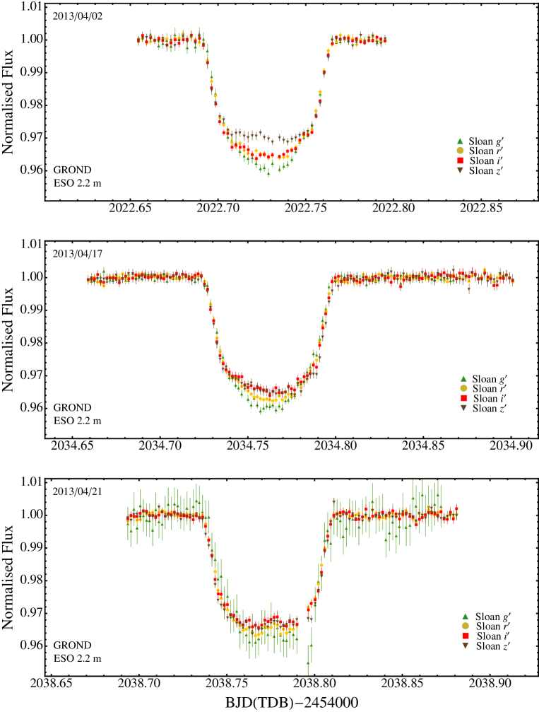
Figure 1: Light curves of three transits of Qatar-2 b observed simultaneously in four optical bands with GROND, ordered according to date.

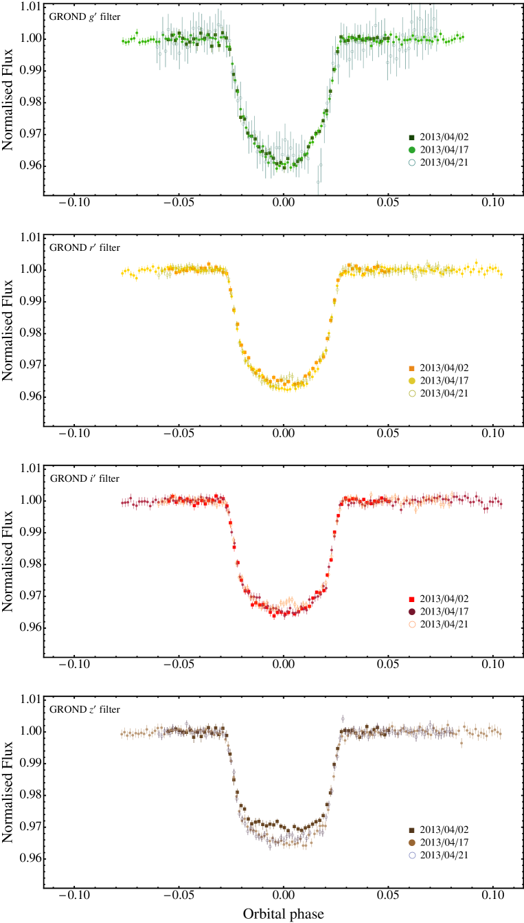
Figure 2: Phased light curves of the three transits of Qatar-2 b observed with GROND, ordered according to the filter used. This highlights the anomalies between the three transits in each colour.

In this section we describe the methodologies used to obtain accurate photometric observations of transiting-planet events and get reliable physical information on the planetary system.

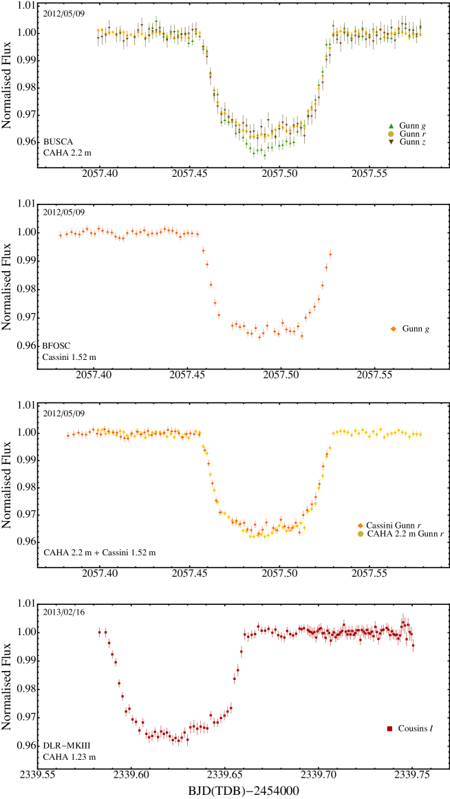
Figure 3: Light curves of two transits of Qatar-2 b observed with three telescopes, shown in date order. Top panel: light curves of one transit of Qatar-2 b observed simultaneously in three optical bands with BUSCA at the CAHA 2.2 m telescope. The anomalies on the light curves are interpreted as the occultation of a starspot by the planet. Second panel: light curve obtained with the Cassini 1.52 m telescope using a Gunn $r$ filter. This is the same transit observed with BUSCA. Third panel: CAHA 2.2 m and Cassini 1.5 m Gunn-$r$ light curves. Bottom panel: light curve obtained with the CAHA 1.23 m telescope using a Cousin $I$ filter.

Table 1: Details of the transit observations presented in this work. $N_{\rm obs}$ is the number of observations, $T_{\rm exp}$ is the exposure time, $T_{\rm obs}$ is the observational cadence, and ‘Moon illum.’ is the fractional illumination of the Moon at the midpoint of the transit. The aperture sizes are the radii of the software apertures for the star, inner sky and outer sky, respectively. Scatter is the r.m.s. scatter of the data versus a fitted model. $\beta$ is the ratio between the noise levels due to Poisson noise and to combined Poisson and red noise.

Telescope	Date of	Start time	End time	$N_{\rm obs}$	$T_{\rm exp}$	$T_{\rm obs}$	Filter	Airmass	Moon	Aperture	Scatter	$\beta$
	first obs.	(UT)	(UT)		(s)	(s)			illum.	radii (px)	(mmag)
ESO 2.2 m #1	2012 04 02	03:34	06:56	61	120	200	Sloan $g^{\prime}$	$1.25\rightarrow 1.08\rightarrow 1.14$	$83\%$	23, 45, 75	1.22	1.26
ESO 2.2 m #1	2012 04 02	03:34	06:56	61	120	200	Sloan $r^{\prime}$	$1.25\rightarrow 1.08\rightarrow 1.14$	$83\%$	29, 55, 85	0.78	1.00
ESO 2.2 m #1	2012 04 02	03:34	06:56	61	120	200	Sloan $i^{\prime}$	$1.25\rightarrow 1.08\rightarrow 1.14$	$83\%$	29, 55, 85	0.88	1.06
ESO 2.2 m #1	2012 04 02	03:34	06:56	61	120	200	Sloan $z^{\prime}$	$1.25\rightarrow 1.08\rightarrow 1.14$	$83\%$	30, 55, 85	0.99	1.15
ESO 2.2 m #2	2012 04 17	03:38	09:26	138	124	150	Sloan $g^{\prime}$	$1.13\rightarrow 1.08\rightarrow 2.70$	$9\%$	29, 55, 85	0.96	1.00
ESO 2.2 m #2	2012 04 17	03:38	09:26	138	124	150	Sloan $r^{\prime}$	$1.13\rightarrow 1.08\rightarrow 2.70$	$9\%$	34, 55, 85	0.74	1.42
ESO 2.2 m #2	2012 04 17	03:38	09:26	138	124	150	Sloan $i^{\prime}$	$1.13\rightarrow 1.08\rightarrow 2.70$	$9\%$	33, 55, 85	0.84	1.55
ESO 2.2 m #2	2012 04 17	03:38	09:26	138	124	150	Sloan $z^{\prime}$	$1.13\rightarrow 1.08\rightarrow 2.70$	$9\%$	30, 55, 85	1.01	1.46
ESO 2.2 m #3	2012 04 21	04:28	08:58	102	124	150	Sloan $g^{\prime}$	$1.08\rightarrow 2.46$	$1\%$	28, 55, 85	3.26	1.60
ESO 2.2 m #3	2012 04 21	04:28	08:58	102	124	150	Sloan $r^{\prime}$	$1.08\rightarrow 2.46$	$1\%$	35, 60, 90	0.77	1.40
ESO 2.2 m #3	2012 04 21	04:28	08:58	102	124	150	Sloan $i^{\prime}$	$1.08\rightarrow 2.46$	$1\%$	32, 60, 90	0.93	1.32
ESO 2.2 m #3	2012 04 21	04:28	08:58	102	124	150	Sloan $z^{\prime}$	$1.08\rightarrow 2.46$	$1\%$	32, 60, 90	1.02	1.12
CAHA 2.2 m	2012 05 09	21:25	01:43	89	120	200	Gunn $g$	$1.50\rightarrow 1.40\rightarrow 2.15$	$79\%$	15, 55, 80	1.65	1.18
CAHA 2.2 m	2012 05 09	21:25	01:43	89	120	200	Gunn $r$	$1.50\rightarrow 1.40\rightarrow 2.15$	$79\%$	15, 50, 80	0.92	1.17
CAHA 2.2 m	2012 05 09	21:25	01:43	89	120	200	Gunn $z$	$1.50\rightarrow 1.40\rightarrow 2.15$	$79\%$	20, 40, 55	1.70	1.01
Cassini 1.52 m	2012 05 09	21:01	00:28	64	170	180	Gunn $r$	$1.64\rightarrow 1.57\rightarrow 2.11$	$80\%$	28, 55, 85	0.80	1.12
CAHA 1.23 m	2013 02 16	01:53	05:54	128	140	180	Cousin $I$	$1.74\rightarrow 1.40\rightarrow 1.55$	$33\%$	20, 45, 60	1.36	1.26

2.1 Telescope defocussing observations of planetary transits

All the observations presented in this work were performed using the telescope-defocussing technique (Alonso et al., 2008; Southworth et al., 2009). In this method the telescope is defocussed so point spread functions (PSFs) cover of order 1000 pixels, and long exposure times (up to $\sim 120$ s) are used to collect many photons in each PSF. This increases the observational efficiency as the CCD is read out less often, thus minimising Poisson and scintillation noise. The large PSFs are also insensitive to focus or seeing changes, which might otherwise cause systematic errors. The other main source of systematic error, flat-fielding, is decreased by two orders of magnitude as each PSF covers of order $10^{3}$ pixels. Telescope pointing errors affect photometry via flat-fielding errors, so these also average down to very low levels.

The exposure time is chosen for a given observing sequence from consideration of the brightness of the target and comparison stars, sky background, telescope size and filter used. The amount of defocussing is then tuned so the peak count rate in the PSFs of the target and comparison stars is significantly below the onset of nonlinearity effects in the CCD. Changes in seeing, airmass and sky transparency affect the count rate of the observations; this is accounted for by changing the exposure times but not the focus setting during an observing sequence.

2.2 Two-site observations of planetary transits

Time-series photometry of transit events can show anomalies due to the planet crossing over spots on the stellar surface. The detection of starspots occulted by a transiting planet is becoming commonplace (e.g. Pont et al., 2007; Rabus et al., 2009; Silva-Valio et al., 2010; Désert, 2011; Sanchis-Ojeda et al., 2011; Sanchis-Ojeda & Winn, 2011; Tregloan-Reed et al., 2013; Mohler-Fischer et al., 2013; Mancini et al., 2013c). However, in the case of ground-based observations, similar signals could be caused by weather-related or instrumental effects. One method to sift the astrophysical from observational anomalies is to observe a transit event from multiple telescopes at different observatories. Any feature present in all light curves is unambiguously intrinsic to the target of the observations. We used this strategy to observe a transit of Qatar-2 using two telescopes at different locations.

This two-site observational strategy was successfully tested in the follow-up of HAT-P-8, where an anomaly was detected in both the light curves (Mancini et al., 2013a). It was also used for HAT-P-16 and WASP-21 (Ciceri et al., 2013), although in these two cases no anomalies were detected. Conversely, Lendl et al. (2013) used this method to show that a possible starspot anomaly in the WASP-19 system was of instrumental origin.

2.3 Multi-band observations of planetary transits

Precise photometric observations of planetary transits probe the chemical composition of the atmosphere of TEPs in a way similar to transmission spectroscopy. A dependence of opacity on wavelength causes variations in the radius of the planet as found from transit observations. The effect can be big enough to measure using medium-size telescopes with multi-band imagers, assuming they have a good spectral resolution. It is important to obtain the observations at multiple wavelengths simultaneously, to avoid variations in transit depth due to unseen starspots rather than planetary radius variations, even if one should take into account that unocculted star spots may still cause wavelength dependence of the transit depth (Sing et al., 2011). In order to investigate this effect, one should monitor the variability of the parent star for many years or, assuming that stellar activity does not change suddenly, repeatedly measure the transit depth by observing several planetary-transit events a few days away from each other.

Simultaneous multi-band observations also allow a detailed study of starspots which are occulted by the transiting planet. For a single light curve the spot radius is strongly correlated with its temperature (e.g. Tregloan-Reed et al., 2013). Multi-band light curves constrain the spot temperature relative to the effective temperature ($T_{\rm eff}$) of the pristine photosphere, thus providing additional information which lifts this degeneracy.

Simultaneous multi-band observations of planetary transits have been obtained for several TEP systems using the instruments BUSCA (Southworth et al., 2012b; Mancini et al., 2013a), GROND (de Mooij et al., 2012; Mancini et al., 2013b, c; Nikolov et al., 2013; Southworth et al., 2013; Penev et al., 2013; Mohler-Fischer et al., 2013; Bayliss et al., 2013), ULTRACAM (Copperwheat et al., 2013; Bento et al., 2013) and SIRIUS (Narita et al., 2013).

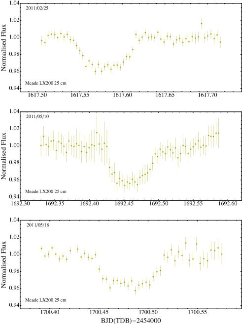
Figure 4: Three transit events of Qatar-2 b observed in 2011 with a 25-cm MEADE LX200 telescope at the Canis Mayor observatory.

3 Observations and data reduction

Five transits of Qatar-2 b were monitored at optical wavelengths by five different telescopes in 2012 and 2013 (Table 1). One transit was followed simultaneously by two of the telescopes, one was simultaneously observed through three filters, and the other three through four filters. All observations were performed with autoguiding and defocussing. The light curves are given in Table 2 and shown in Figs. 1, 2 and 3. We obtained observations of three more transits in 2011 with a 25 cm telescope (Fig. 4).

All observations were analysed with the defot pipeline (Southworth et al., 2009) written in idl. Debiasing and flat-fielding were done using master calibration frames obtained by median-combining individual calibration images. Pointing variations were corrected by cross-correlating each image against a reference frame. No de-correlation with PSF location was necessary because, due to defocussing, the PSFs are much bigger than the pixel sizes of the CCDs and image motion as the telescopes tracked. Apertures were placed by hand on the target and comparison stars, and their radii were chosen based on the lowest scatter achieved when compared with a fitted model.

The aper routine used to measure the differential photometry commonly returns underestimated errorbars. We therefore enlarged the errorbars for each light curve to give a reduced $\chi^{2}$ of $\chi_{\nu}^{2}=1$ versus a fitted model. We then further inflated the errorbars using the $\beta$ approach (e.g. Gillon et al. 2006; Winn et al. 2008; Gibson et al. 2008) to account for any correlated noise. We calculated $\beta$ values for between two and ten data points for each light curve, and adopted the largest $\beta$ value. They are reported in Table 1.

The twelve GROND light curves are plotted according to date (Fig. 1) and filter (Fig. 2) in order to highlight the starspot anomalies found in each transit.

Table 2: Excerpts of the light curves of Qatar-2: this table will be made available at the CDS. A portion is shown here for guidance regarding its form and content.

Telescope	Filter	BJD(TDB)	Diff. mag.	Uncertainty
ESO 2.2 m #1	$g^{\prime}$	2456022.654686	0.000290	0.001370
ESO 2.2 m #1	$g^{\prime}$	2456022.656996	-0.001152	0.001314
ESO 2.2 m #2	$r^{\prime}$	2456034.658998	0.001033	0.001019
ESO 2.2 m #2	$r^{\prime}$	2456034.660816	0.000272	0.001015
ESO 2.2 m #3	$i^{\prime}$	2456038.693584	0.001068	0.001281
ESO 2.2 m #3	$i^{\prime}$	2456038.695359	0.000085	0.001276
CAHA 2.2 m	$z$	2456057.399202	0.001767	0.002883
CAHA 2.2 m	$z$	2456057.401301	0.001192	0.002921
Cassini 1.52 m	$r$	2456057.382333	0.000839	0.001281
Cassini 1.52 m	$r$	2456057.385550	0.000361	0.001184
CAHA 1.23 m	$I$	2456339.583029	-0.000127	0.001653
CAHA 1.23 m	$I$	2456339.586323	-0.000021	0.001636

3.1 MPG/ESO 2.2-m telescope

Three transits of Qatar-2 b were monitored with the GROND instrument mounted on the MPG/ESO 2.2 m telescope at the ESO observatory in La Silla, Chile. The transit events were observed on 2012 April 2, 17 and 21. GROND is an imaging system capable of simultaneous photometric observations in four fixed optical (similar to Sloan $g^{\prime}$, $r^{\prime}$, $i^{\prime}$, $z^{\prime}$) and three fixed NIR ($J,\,H,\,K$) passbands (Greiner et al., 2008). Each of the four optical channels is equipped with a back-illuminated $2048\times 2048$ E2V CCD, with a field-of-view (FOV) of $5.4^{\prime}\times 5.4^{\prime}$ at a scale of $0.158^{\prime\prime}/\rm{pixel}$. The three NIR channels use $1024\times 1024$ Rockwell HAWAII-1 arrays with a FOV of $10^{\prime}\times 10^{\prime}$ at $0.6^{\prime\prime}/\rm{pixel}$. Unfortunately, due to a lack of good reference stars in the FOV, we were not able to obtain usable light curves in the three NIR bands.

The precision of the optical data are in agreement with the statistical-uncertainty study performed by Pierini et al. (2012) with two exceptions. The $z^{\prime}$ transit observed on 2012 April 2 has a lower depth compared to the other light curves of the same transit (upper panel of Fig. 1) or the $z^{\prime}$ light curves of the other two transits (bottom panel of Fig. 2). This was caused by an unknown instrumental error, which could not be reliably corrected for during the data reduction. The $g^{\prime}$ data observed on 2012 April 21 were affected by excess readout noise, caused by another unknown instrumental problem, so are very inaccurate compared to the other three light curves of this transit (bottom panel of Fig. 1) or to the $g^{\prime}$ light curves of the other two transits (upper panel of Fig. 2).

3.2 CAHA 2.2-m telescope

We observed one full transit on the night of 2012 May 9, using the CAHA 2.2-m telescope and BUSCA imager at the German-Spanish Astronomical Center at Calar Alto in Spain. BUSCA is designed for simultaneous four-colour photometry and, unlike GROND, the user has a choice of filters available for each arm. Each of the four optical channels is equipped with a Loral CCD4855 4k$\times$4k CCD with 15$\times$15 $\mu$m pixels, providing an astronomical FOV of nearly 12$\times$12 arcmin.

For our observations we selected a Strömgren $u$ filter in the bluest arm and standard Calar Alto Gunn $g$, $r$ and $z$ filters in the other three arms. This choice led to a reduced field of view (from $12^{\prime}\times 12^{\prime}$ to a circle of $6^{\prime}$ in diameter), but had two advantages. Firstly the $g$ and $r$ filters have a much better throughput compared to the default Strömgren $b$ and $y$ filters. Secondly, the different filter thicknesses meant the $u$ band, where the target star is comparatively faint, was less defocussed. The CCDs were binned $2\times 2$ to shorten the readout time. The autoguider was operated in focus. Unfortunately, the data obtained in the $u$ band were too strongly affected by atmospheric extinction and poor signal-to-noise ratio to be useful. The $g$, $r$ and $z$ light curves are plotted in Fig. 3.

3.3 Cassini 1.52-m telescope

The transit event of 2012 May 9 was also observed with the BFOSC (Bologna Faint Object Spectrograph & Camera) imager mounted on the 1.52 m Cassini Telescope at the Astronomical Observatory of Bologna in Loiano, Italy. The transit was not fully covered due to the pointing limits of the telescope. The CCD was used unbinned, giving a plate scale of $0.58^{\prime\prime}/\rm{pixel}$, for a total FOV of $13^{\prime}\times 12.6^{\prime}$. A Gunn $r$ filter was used. The CCD was windowed to decrease the readout time and the telescope was autoguided and defocussed, allowing low scatter to be obtained even though the observations were conducted at high airmass (see Table 1). The light curve is plotted in Fig. 3. The Cassini data are consistent with the presence of the starspot anomaly in the final phase of the transit ingress.

3.4 CAHA 1.23-m telescope

Another complete transit event was observed with the CAHA 1.23 m telescope, on the night of 2013 February 16. Mounted in the Cassergrain focus of this telescope is the DLR-MKIII camera, which has $4000\times 4000$ pixels, a plate scale of 0.32 arcsec pixel^-1 and a large FOV of $21.5^{\prime}\times 21.5^{\prime}$. The transit was monitored through a Cousins-$I$ filter, the telescope was autoguided and defocussed, and the CCD was windowed. The resulting light curve is plotted in Fig. 3. An anomaly is also visible in this light curve, shortly after the transit midpoint.

3.5 Canis Mayor Observatory

Three complete transits were observed at the Canis Mayor Observatory, located in Castelnuovo Magra, Italy. The instrument used for the observations was a Meade LX200 GPS 10 inch telescope, equipped with an f/6.3 focal reducer and an SBIG ST8 XME CCD camera. Science frames were taken through the Baader Yellow 495 Longpass filter and the exposure time was 300 s. The telescope was autoguided and slightly defocussed. The light curves are plotted in Fig. 4.

4 Light-curve analysis

All of our high-precision light curves show possible starspot crossing events, which must be analysed using a self-consistent and physically realistic model. We use the prism and gemc codes (Tregloan-Reed et al., 2013) for this. We have previously used these codes to model HATS-2 (Mohler-Fischer et al., 2013) and WASP-19 (Mancini et al., 2013c).

prism models planetary transits with starspot crossings using a pixellation approach in Cartesian coordinates. gemc uses a Differential Evolution Markov Chain Monte Carlo (DE-MCMC) approach to locate the parameters of the prism model which best fit the data, using a global search. prism uses the fractional radii, $r_{\mathrm{A}}=\frac{R_{\mathrm{A}}}{a}$ and $r_{\mathrm{b}}=\frac{R_{\mathrm{b}}}{a}$, where $R_{\mathrm{A}}$ and $R_{\mathrm{b}}$ are the true radii of the star and planet, and $a$ is the orbital semimajor axis.

The fitted parameters of prism are the sum and ratio of the fractional radii ($r_{\mathrm{A}}+r_{\mathrm{b}}$ and $k=\frac{r_{\mathrm{b}}}{r_{\mathrm{A}}}$), the orbital period and inclination ($P$ and $i$), the time of transit midpoint ($T_{0}$) and the two coefficients of the quadratic limb darkening (LD) law ($u_{\mathrm{A}}$ and $v_{\mathrm{A}}$). Each starspot is represented by the longitude and colatitude of its centre ($\theta$ and $\phi$), its angular radius ($r_{\mathrm{spot}}$) and its contrast ($\rho_{\mathrm{spot}}$), the latter being the ratio of the surface brightness of the starspot to that of the surrounding photosphere.

The datasets obtained with the 25-cm telescope were modelled using the much faster jktebop code, as no starspot anomalies are visible. The parameters used for jktebop were the same as for prism.

4.1 Orbital period determination

Table 3: Times of transit midpoint of Qatar-2 b and their residuals. TRESCA refer to the “TRansiting ExoplanetS and CAndidates”. References: (1) Canis Major Observatory (this work); (2) Bryan et al. (2012); (3) Strajnic et al. (TRESCA); (4) Zibar M. (TRESCA); (5) Gonzales J. (TRESCA); (6) MPG/ESO 2.2-m $g^{\prime}$ (this work); (7) MPG/ESO 2.2-m $r^{\prime}$ (this work); (8) MPG/ESO 2.2-m $i^{\prime}$ (this work); (9) MPG/ESO 2.2-m $z^{\prime}$ (this work); (10) Dax T. (TRESCA); (11) Masek M. (TRESCA); (12) Carreno A. (TRESCA); (13) Montigiani N., Manucci M. (TRESCA); (14) Cassini 1.52-m (this work); (15) CAHA 2.2-m $g$ (this work); (16) CAHA 2.2-m $r$ (this work); (17) CAHA 2.2-m $z$ (this work); (18) Campbell J. (TRESCA); (19) CAHA 1.23-m (this work); (20) René R. (TRESCA); (21) Ayiomamitis A. (TRESCA); (22) Jacobsen J. (TRESCA); (23) Kehusmaa P., Harlingten C. (TRESCA); (24) Shadic S. (TRESCA); (25) Colazo C. et al. (TRESCA).

Time of minimum	Cycle	Residual	Reference
BJD(TDB)$-2400000$	no.	(JD)
$55617.58156\pm 0.00082$	-5	0.00005	1
$55624.26679\pm 0.00011$	0	-0.00031	2
$55692.46109\pm 0.00270$	51	0.00105	1
$55700.47915\pm 0.00083$	57	-0.00358	1
$55974.59334\pm 0.00072$	262	0.00173	3
$55978.60480\pm 0.00120$	265	0.00184	4
$55986.62711\pm 0.00069$	271	0.00145	5
$56022.72850\pm 0.00018$	298	0.00070	6
$56022.72800\pm 0.00017$	298	0.00020	7
$56022.72815\pm 0.00016$	298	0.00035	8
$56022.72810\pm 0.00022$	298	0.00030	9
$56026.73842\pm 0.00033$	301	-0.00073	10
$56030.75160\pm 0.00150$	304	0.00110	11
$56034.76157\pm 0.00010$	307	-0.00028	6
$56034.76196\pm 0.00012$	307	0.00011	7
$56034.76198\pm 0.00015$	307	0.00013	8
$56034.76249\pm 0.00015$	307	0.00064	9
$56037.43785\pm 0.00068$	309	0.00176	12
$56038.77329\pm 0.00010$	310	0.00009	7
$56038.77345\pm 0.00012$	310	0.00025	8
$56038.77312\pm 0.00015$	310	-0.00008	9
$56045.45890\pm 0.00042$	315	0.00012	13
$56057.49242\pm 0.00018$	324	-0.00041	14
$56057.49246\pm 0.00028$	324	-0.00037	15
$56057.49274\pm 0.00016$	324	-0.00009	16
$56057.49282\pm 0.00023$	324	-0.00012	17
$56336.94926\pm 0.00059$	533	-0.00091	18
$56339.62434\pm 0.00027$	535	0.00007	19
$56343.63460\pm 0.00110$	538	-0.00116	20
$56394.44559\pm 0.00056$	576	-0.00059	21
$56410.49050\pm 0.00100$	588	-0.00108	22
$56411.83020\pm 0.00058$	589	-0.00150	23
$56419.85020\pm 0.00130$	595	-0.00120	24
$56442.58191\pm 0.00014$	612	-0.00047	25

Figure 5: Plot of the residuals of the times of transit midpoint of Qatar-2 b versus a linear ephemeris. The timings plotted with diamonds are from this work, while empty circles are from ETD and the box is from Bryan et al. (2012). The box has the same size of the corresponding error bar, which has been suppressed for clarity.

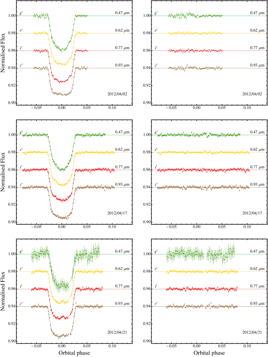
Figure 6: Phased GROND light curves of Qatar-2 compared to the best prism+gemc fits. The light curves and the residuals are ordered according to the central wavelength of the filter used. The passbands are labelled on the left of the figure, and their central wavelengths are given on the right.

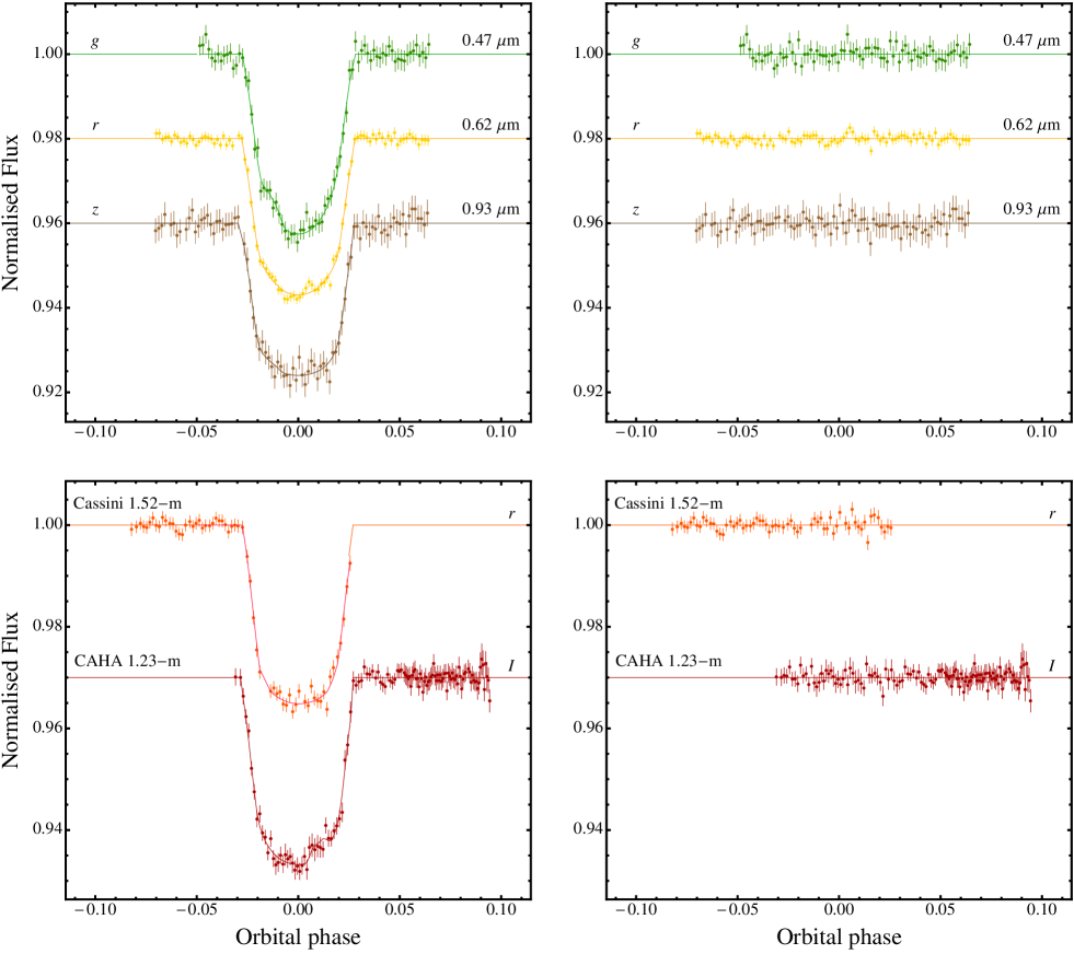
Figure 7: Top panels: phased BUSCA light curves of Qatar-2 compared to the best prism+gemc fits. The light curves are ordered according to the central wavelength of the filter used. The passbands are labelled on the left of the figure, and their central wavelengths are given on the right. Bottom panels: as above, but for the Cassini 1.52-m and the CAHA 1.23-m telescopes. The residuals of each fit are plotted in the right panels.

We used the photometric data presented in Sect. 3 to refine the orbital period of Qatar-2 b. We excluded the third $g^{\prime}$-band transit observed with GROND due to the large scatter of these data. The transit times and uncertainties for the high-precision datasets were obtained using prism+gemc. Those for the small telescope were calculated using jktebop and Monte Carlo simulations. To these timings we added one from the discovery paper (Bryan et al., 2012) and 14 measured by amateur astronomers and available on the ETD website. The ETD light curves were included only if they had complete coverage of the transit and a Data Quality index $\leq 3$. All 34 timings were placed on the BJD(TDB) time system (Table 3).

Possible unknown planets in the system could gravitationally perturb the orbit of Qatar-2 b and induce transit timing variations (TTVs). We therefore searched for periodic variations in the transit times that might indicate such perturbations. We first performed a weighted linear least-squares fit to compute a new system ephemeris of $T_{\mathrm{T}}=T_{0}+P\times E$, where $E$ is the number of orbital cycles after the reference epoch and

$$T_{0}=\mathrm{BJD(TDB)}2\,455\,624.267096\pm 0.000087,$$

$$P=1.33711647\pm 0.00000026\,\mathrm{d}$$

and the covariance between the two parameters is $-2.11\times 10^{-11}$ d². A plot of the residuals around the fit is shown in Fig. 5. We then look for sinusoidal variations in the residuals by scanning through a wide range of periods (10–1000 orbits of Qatar-2 b) and looking for the best-fitting sinusoid at each period. Across this range of periods, the best-fitting sinusoid has a period of 11.8 d, but there are a large range of local minima in the interval $15-200$ orbits. All of these candidate TTV signals give $\chi^{2}\sim 100$, implying that our sinusoidal TTV models fit the data only poorly. The semi-amplitudes of these best-fitting TTV models are all $\sim$30 sec, so we quote this value as the nominal upper limit of any TTV effects on the orbit of Qatar-2b.

4.2 Light-curve modelling

From this point we considered only the high-precision light curves (i.e. not the Canis-Mayor ones). These were individually modelled with prism+gemc, each time including the parameters for one starspot. We used GEMC to randomly generate parameters for 36 chains, within a reasonable initial parameter space, and then to simultaneously evolve the chains for 50 000 successive generations; see Tregloan-Reed et al. (2013) for details. The light curves and their best-fitting models are shown in Figs. 6 and 7. The derived parameters of the planetary system are reported in Table 4, while those of the starspots in Table 5. We used the former to reanalyse the phsyical properties of the system (Sect. 5), and the latter for the characterisation of the starspots and the planetary orbit (Sect. 6).

The results concerning the first GROND $z^{\prime}$ data set were not considered since these data were compromised by an instrumental error (Sect. 3.1). Due to its low quality, the starpsot parameters resulted from the fit of the third GROND $g^{\prime}$ light curve have very large error bars and were not reported in Table 5.

We compared the fitted LD coefficients with the expected stellar atmosphere model values. For the $g^{\prime}$, $r^{\prime}$, $i^{\prime}$, $z^{\prime}$ and $I$ bands, we used the theoretical LD coefficients estimated by Claret (2004) with two different model atmosphere codes (atlas and phoenix). We also checked the values for other passbands ($V$, $R_{\mathrm{c}}$, $I_{\mathrm{c}}$, $R_{\mathrm{j}}$, $I_{\mathrm{j}}$), where predictions from different authors (van Hamme, 1993; Diaz-Cordoves et al., 1995; Claret, 2000) are available. While there is a good agreement for most of the light curves, there are some, especially those related to the $g^{\prime}$ band, for which differences of $\pm 0.1$ up to $\pm 0.3$ are apparent. Moreover, one has also to consider that starspots do affect LD coefficients as spots have different LD to the rest of the star (Ballerini et al., 2012). Based on these arguments, we could not assume that theoretical LD coefficients are correct, and we preferred to fit for the coefficients using prism+gemc.

We discounted all the $g$-band data sets because the best-fitting models returned very large value for $k$ compared to those of the other redder bands. Considering the high activity level of Qatar-2 A, as can be seen from the numerous occulted starspots detected, we attribute this to the effect of unocculted starspots (i.e. starspots in a region of the stellar disc is not crossed by the planet) which cause the transits monitored in the bluest bands to be deeper. This is easily seen in Fig. 8 in which, using Eq. (4) and (5) from Sing et al. (2011), we plot for the case of Qatar-2 the correction for unocculted spots for a total dimming of $1\%$ at a reference wavelength of 600 nm for different starspot temperatures. Starspots are modelled with atlas9 stellar atmospheric models (Kurucz, 1979) of different temperatures ranging from 4450 to 3700 K in 250 K intervals, and $T_{\mathrm{eff}}=4645$ K for the stellar temperature. However, in order to apply the right correction for unocculted starspot, we need an estimate of the absolute level of the stellar flux corresponding to a spot-free surface, which can be obtained through a continuing, accurate photometric monitoring of Qatar-2 A over several years. Since the QES discovery data are not public and no other long photometric monitoring are available for this target, we decided to exclude the $g$-band data for the estimation of the physical parameters of the system. Instead, corrections on the other optical bands ($\lambda>540$ nm) are expected to be of the order of $\lesssim 10^{-3}$, adding only a small contribution to the uncertainties in the $k$ values.

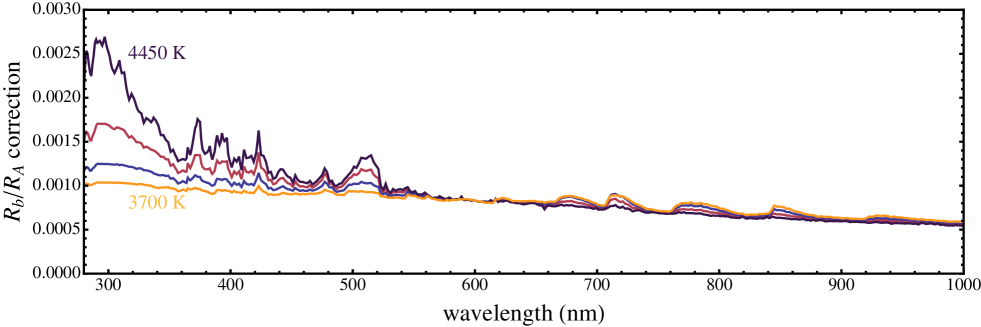
Figure 8: The effect of unocculted starspots on the transmission spectrum of Qatar-2 considering a $1\%$ flux drop at 600 nm. A grid of atlas9 stellar atmospheric models at different temperature, ranging from 4450 to 3700 K in 250 K intervals, was used to model the starspot coverage, while for the star a model with $T_{\mathrm{eff}}=4645$ K was adopted.

Table 4: Parameters of the prism+gemc best fits of the light curves of Qatar-2 for the quadratic LD law with the coefficients included as fitted parameters. The final parameters, given in bold, are the weighted means of the results for the individual datasets, but excluding the $g$-band ones (see text). Results from the discovery paper are included at the base of the table for comparison. The orbital period for each data set is reported in Table 3. The results concerning the GROND $z^{\prime}$ dataset of the first transit are not reported (see text).

Telescope	Filter	$r_{\mathrm{A}}+r_{\mathrm{b}}$	$k$	$i^{\circ}$	$u_{\mathrm{A}}$	$v_{\mathrm{A}}$
ESO 2.2-m #1	Sloan $g^{\prime}$	$0.1933\pm 0.0045$	$0.1695\pm 0.0019$	$85.93\pm 0.46$	$0.275\pm 0.039$	$0.652\pm 0.061$
ESO 2.2-m #1	Sloan $r^{\prime}$	$0.1964\pm 0.0036$	$0.1653\pm 0.0016$	$85.62\pm 0.39$	$0.504\pm 0.048$	$0.187\pm 0.022$
ESO 2.2-m #1	Sloan $i^{\prime}$	$0.1929\pm 0.0022$	$0.1663\pm 0.0011$	$86.20\pm 0.26$	$0.431\pm 0.044$	$0.182\pm 0.017$
ESO 2.2-m #2	Sloan $g^{\prime}$	$0.2013\pm 0.0070$	$0.1720\pm 0.0043$	$85.09\pm 0.78$	$0.712\pm 0.106$	$0.077\pm 0.011$
ESO 2.2-m #2	Sloan $r^{\prime}$	$0.1935\pm 0.0028$	$0.1681\pm 0.0018$	$86.05\pm 0.35$	$0.580\pm 0.060$	$0.111\pm 0.015$
ESO 2.2-m #2	Sloan $i^{\prime}$	$0.1936\pm 0.0025$	$0.1642\pm 0.0014$	$86.25\pm 0.31$	$0.349\pm 0.044$	$0.331\pm 0.045$
ESO 2.2-m #2	Sloan $z^{\prime}$	$0.2003\pm 0.0027$	$0.1641\pm 0.0016$	$86.00\pm 0.28$	$0.261\pm 0.042$	$0.564\pm 0.074$
ESO 2.2-m #3	Sloan $g^{\prime}$	$0.1956\pm 0.0134$	$0.1704\pm 0.0057$	$85.42\pm 1.23$	$0.479\pm 0.218$	$0.249\pm 0.229$
ESO 2.2-m #3	Sloan $r^{\prime}$	$0.1947\pm 0.0020$	$0.1658\pm 0.0019$	$86.11\pm 0.26$	$0.588\pm 0.073$	$0.137\pm 0.025$
ESO 2.2-m #3	Sloan $i^{\prime}$	$0.1960\pm 0.0017$	$0.1647\pm 0.0017$	$85.89\pm 0.18$	$0.423\pm 0.144$	$0.141\pm 0.235$
ESO 2.2-m #3	Sloan $z^{\prime}$	$0.1951\pm 0.0015$	$0.1670\pm 0.0010$	$86.17\pm 0.18$	$0.291\pm 0.038$	$0.234\pm 0.032$
CAHA 2.2-m	Gunn $g$	$0.1970\pm 0.0056$	$0.1733\pm 0.0029$	$85.93\pm 0.58$	$0.629\pm 0.060$	$0.315\pm 0.046$
CAHA 2.2-m	Gunn $r$	$0.1948\pm 0.0016$	$0.1676\pm 0.0012$	$86.17\pm 0.18$	$0.543\pm 0.043$	$0.144\pm 0.023$
CAHA 2.2-m	Gunn $z$	$0.1991\pm 0.0053$	$0.1671\pm 0.0024$	$86.05\pm 0.55$	$0.260\pm 0.055$	$0.488\pm 0.089$
Cassini 1.52-m	Gunn $r$	$0.1926\pm 0.0039$	$0.1661\pm 0.0023$	$86.15\pm 0.43$	$0.367\pm 0.146$	$0.250\pm 0.243$
CAHA 1.23-m	Cousins $I$	$0.1992\pm 0.0027$	$0.1665\pm 0.0025$	$86.19\pm 0.35$	$0.441\pm 0.135$	$0.337\pm 0.200$
Final results		$\mathbf{0.19549\pm 0.00065}$	$\mathbf{0.16590\pm 0.00044}$	$\mathbf{86.12\pm 0.08}$
Bryan et al. (2012)			$0.16508\pm 0.00080$	$88.30\pm 0.94$

Table 5: Starspot parameters derived from the prism+gemc fitting of the transit light curves presented in this work.
^(a)The longitude of the centre of the spot is defined to be $0^{\circ}$ at the centre of the stellar disc and can vary from $-90^{\circ}$ to $90^{\circ}$. ^(b)The colatitude of the centre of the spot is defined to be $0^{\circ}$ at the north pole and $180^{\circ}$ at the south pole. ^(c)Angular radius of the starspot; note that $90^{\circ}$ degrees covers half of stellar surface. ^(d)Spot contrast; note that 1.0 equals the brightness of the surrounding photosphere. ^(e)The temperature of the starspots are obtained by considering the photosphere and the starspots as black bodies (see text in Sect. 6). The results concerning the GROND $z^{\prime}$ dataset of the first transit are not reported, because this dataset is affected by correlated noise. Due to very large uncertainties, the results concerning the GROND $g^{\prime}$ dataset of the third transit are not reported. The results for the Cassini data set are also not reported due to the large uncertainties of the parameters due to the fact that the light-curve points are very scattered during the transit time and the sampling is not so good.

Telescope	Filter	$\theta(^{\circ})\,^{a}$	$\phi(^{\circ})\,^{b}$	$r_{\rm spot}(^{\circ})\,^{c}$	$\rho_{\rm spot}\,^{d}$	Temperature (K)$\,{}^{e}$
ESO 2.2-m #1	Sloan $g^{\prime}$	$37.67\pm 2.65$	$73.98\pm 2.44$	$6.26\pm 0.64$	$0.392\pm 0.066$	$4068\pm 99$
ESO 2.2-m #1	Sloan $r^{\prime}$	$36.50\pm 6.12$	$80.34\pm 7.27$	$6.07\pm 0.97$	$0.540\pm 0.091$	$4137\pm 130$
ESO 2.2-m #1	Sloan $i^{\prime}$	$37.71\pm 2.53$	$73.63\pm 5.61$	$3.09\pm 0.26$	$0.579\pm 0.052$	$4096\pm 89$
ESO 2.2-m #2	Sloan $g^{\prime}$	$-32.70\pm 3.38$	$66.50\pm 10.17$	$4.48\pm 0.51$	$0.468\pm 0.049$	$4166\pm 72$
ESO 2.2-m #2	Sloan $r^{\prime}$	$-29.64\pm 2.26$	$70.88\pm 4.89$	$4.23\pm 0.48$	$0.588\pm 0.048$	$4201\pm 74$
ESO 2.2-m #2	Sloan $i^{\prime}$	$-32.62\pm 3.70$	$69.30\pm 6.18$	$4.02\pm 0.67$	$0.626\pm 0.087$	$4167\pm 134$
ESO 2.2-m #2	Sloan $z^{\prime}$	$-26.61\pm 3.66$	$67.78\pm 7.35$	$3.24\pm 0.43$	$0.660\pm 0.072$	$4143\pm 125$
ESO 2.2-m #3	Sloan $r^{\prime}$	$4.15\pm 0.48$	$72.89\pm 4.23$	$4.83\pm 0.50$	$0.566\pm 0.091$	$4172\pm 127$
ESO 2.2-m #3	Sloan $i^{\prime}$	$4.70\pm 2.39$	$72.73\pm 4.76$	$4.96\pm 2.76$	$0.556\pm 0.183$	$4061\pm 290$
ESO 2.2-m #3	Sloan $z^{\prime}$	$4.54\pm 0.62$	$70.00\pm 5.74$	$3.76\pm 0.57$	$0.653\pm 0.116$	$4132\pm 196$
CAHA 2.2-m	Gunn $g$	$-30.48\pm 4.13$	$67.76\pm 9.52$	$3.83\pm 0.93$	$0.422\pm 0.102$	$4078\pm 145$
CAHA 2.2-m	Gunn $r$	$-30.89\pm 5.89$	$72.86\pm 9.73$	$3.45\pm 1.63$	$0.563\pm 0.095$	$4144\pm 137$
CAHA 2.2-m	Gunn $z$	$-29.59\pm 6.83$	$84.71\pm 23.14$	$4.84\pm 0.99$	$0.702\pm 0.184$	$4217\pm 292$
CAHA 1.23-m	Cousins $I$	$25.29\pm 9.22$	$68.97\pm 11.26$	$4.72\pm 4.16$	$0.601\pm 0.216$	$4120\pm 332$

5 Physical parameters of the planetary system

We measured the physical properties of the Qatar-2 system using the Homogeneous Studies approach (see Southworth 2012 and references therein). This methodology makes use of the photometric parameters reported in Table 4, spectroscopic parameters from the discovery paper (velocity amplitude $K_{\mathrm{A}}=558.7\pm 5.9$ m s^-1, effective temperature $T_{\mathrm{eff}}=4645\pm 50$ K, metallicity [Fe/H] $=-0.02\pm 0.08$ dex, and eccentricity $e=0$; Bryan et al., 2012) and theoretical stellar models to estimate the properties of the system.

A value was estimated for $K_{\mathrm{b}}$, the velocity amplitude of the planet, and the full system properties were calculated using standard formulae. $K_{\mathrm{b}}$ was then iteratively adjusted to find the best agreement between the observed $r_{\rm A}$ and $T_{\rm eff}$, and the values of $\frac{R_{\rm A}}{a}$ and $T_{\rm eff}$ predicted by a theoretical model of the calculated mass. This was done for a grid of ages from zero to 5 Gyr, and for five different sets of theoretical models, specified in Table LABEL:Table:6). We imposed an upper limit of 5 Gyr because the strong spot activity of the host star implies a young age. The formal best fits are found at the largest possible ages (20 Gyr in this case), which implies that the spectroscopic properties of the host star are not a good match for the stellar density implicitly but strongly constrained by the transit duration (Seager & Mallén-Ornelas, 2003). Given the large number of available light curves, the discrepancy is best investigated by obtaining new spectroscopic measurements of the atmospheric properties of Qatar-2 A.

We found a reasonably good agreement between the results for the five different sets of theoretical stellar models (see Table LABEL:Table:6). The Claret models are the most discrepant, but not by enough to reject these results. We also used a model-independent method to estimate the physical parameters of the system, via a calibration based on detached eclipsing binary stars of mass $<$3$\,{M}_{\odot}$ (Enoch et al., 2010; Southworth, 2011). These empirical results match those found by using the stellar models.

The final set of physical properties was obtained by taking the unweighted mean of the five sets of values obtained using stellar models, and are reported in Table 7. Systematic errors were calculated as the standard deviation of the results from the five models for each output parameter. Table 7 also shows the physical properties found by Bryan et al. (2012), which are of lower precision. Our measurement of the stellar density is $\sim 3.7\sigma$ smaller than that found by Bryan et al. (2012). The effect of this is to yield larger radius measurements for both star and planet, and a 30% lower planetary density.

Table 7: Final physical properties of the Qatar-2 planetary system, compared with results from Bryan et al. (2012). The first error bar for each parameter is the statistical error, which stems from the measured spectroscopic and photometric parameters. The second error bar is the systematic error arising from the use of theoretical stellar models, and is given only for those parameters which have a dependence on stellar theory.

		This work (final)			Bryan et al. (2012)
Stellar mass	$M_{\rm A}$ ($\,{M}_{\odot}$)	0.743 $\pm$	0.020  $\pm$	0.007	$0.740\pm 0.037$
Stellar radius	$R_{\rm A}$ ($\,{R}_{\odot}$)	0.776 $\pm$	0.007  $\pm$	0.003	$0.713\pm 0.018$
Stellar surface gravity	$\log g_{\rm A}$ (cgs)	4.530 $\pm$	0.005  $\pm$	0.001	$4.601\pm 0.018$
Stellar density	$\rho_{\rm A}$ ($\,\rho_{\odot}$)	$1.591\pm 0.016$			$2.05\pm 0.12$
Planetary mass	$M_{\rm b}$ ($\,{M}_{\rm Jup}$)	2.494 $\pm$	0.052  $\pm$	0.016	$2.487\pm 0.086$
Planetary radius	$R_{\rm b}$ ($\,{R}_{\rm Jup}$)	1.254 $\pm$	0.012  $\pm$	0.004	$1.144\pm 0.035$
Planetary surface gravity	$g_{\rm b}$ ( m s-2)	$39.34\pm 0.52$			$43.5\pm 2.2$
Planetary density	$\rho_{\rm b}$ ($\,\rho_{\rm Jup}$)	1.183 $\pm$	0.022  $\pm$	0.004	$1.66\pm 0.13$
Planetary equilibrium temperature	$T_{\rm eq}^{\,\prime}$  (K)	$1344\pm 14$			$1292\pm 19$
Safronov number	$\Theta$	0.1152 $\pm$	0.0017  $\pm$	0.0004	$0.740\pm 0.037$
Orbital semimajor axis	$a$ (AU)	0.02153 $\pm$	0.00019  $\pm$	0.00007	$0.02149\pm 0.00036$

6 Starspot modelling

As explained in Sect. 4, the parameters of the starspots detected in the light curves were fitted together with those of the transit using prism and gemc codes. In this way, we were able to establish the best-fitting position, size, spot contrast and temperature for each of them. The results are summarised in Table 5. The final values for the angular radii of the spots detected in each transit come from the weighted mean of the results in each band. These are reported in Table 8 in km and in percent of the stellar disc.

Table 8: Starspot sizes and temperatures for each of the transits presented in this work.

Telescope	Spot radius (km)	% of the stellar disc	Temperature (K)
ESO 2.2-m #1	$34722\pm 2224$	$\sim 0.41\%$	$4094\pm 59$
ESO 2.2-m #2	$36951\pm 2392$	$\sim 0.47\%$	$4176\pm 45$
ESO 2.2-m #3	$41216\pm 3528$	$\sim 0.58\%$	$4148\pm 100$
CAHA 2.2-m	$39352\pm 5906$	$\sim 0.53\%$	$4124\pm 94$
CAHA 1.23-m	$70271\pm 9628$	$\sim 1.70\%$	$4120\pm 332$

Current knowledge on starspot temperatures is based on results coming from different techniques, such as simultaneous modelling of brightness and colour variations, Doppler imaging, modelling of molecular bands and atomic line-depth ratios. Planetary-transit events offer a more direct way to investigate this topic, especially in the lucky case that the parent star is active and that the planet occults one or more starspots during the transit.

For the current case, we observed starspots in every one of the transits that we monitored with high precision. This suggests that Qatar-2 A could be in a peak of its stellar activity, since no starspots were seen in the four light curves observed between February and March 2011 by Bryan et al. (2012), of which three covered the complete transit event.

Taking advantage of our multi-band photometry, we studied how the starspot contrast changes with passband. Starspots are expected to be darker in the ultraviolet (UV) than in the infrared (IR). From Table 5, it is clear that the starspots are brighter in the redder passbands than in the bluer passbands, for all four simultaneous multi-band observations. Modelling both the photosphere and the starspot as black bodies (Rabus et al., 2009; Sanchis-Ojeda et al., 2011; Mohler-Fischer et al., 2013; Mancini et al., 2013c) and using Eq. 1 of Silva (2003) and $T_{\mathrm{eff}}=4645\pm 50$ (Bryan et al., 2012), we estimated the temperature of the starspots at different bands and reported them in the last column of Table 5. The values of the temperature estimated for each transit are in good agreement between each other within the experimental uncertainties and point to starspots with temperature between 4100 and 4200 K. This can be also noted in Fig. 9, where we compare the spot contrasts calculated by prism+gemc with those expected for a starspot at 4200 K over a stellar photosphere of 4645 K, both modelled with atlas9 atmospheric models (Kurucz, 1979). The weighted means are shown in Table 8, and are consistent with what has been observed for other main-sequence stars (Berdyugina, 2005), and for the case of the TrES-1 (Rabus et al., 2009), CoRoT-2 (Silva-Valio et al., 2010), HD 189733 (Sing et al., 2011), WASP-4 (Sanchis-Ojeda et al., 2011), HATS-2 (Mohler-Fischer et al., 2013) and WASP-19 (Mancini et al., 2013c; Huitson et al., 2013). All these measurements are shown in Fig. 10 versus the temperature of the photosphere of the corresponding star. The spectral class for most of the stars is also reported and allows to see that the temperature difference between photosphere and starspots is not strongly dependent on spectral type, as already noted by Strassmeier (2009).

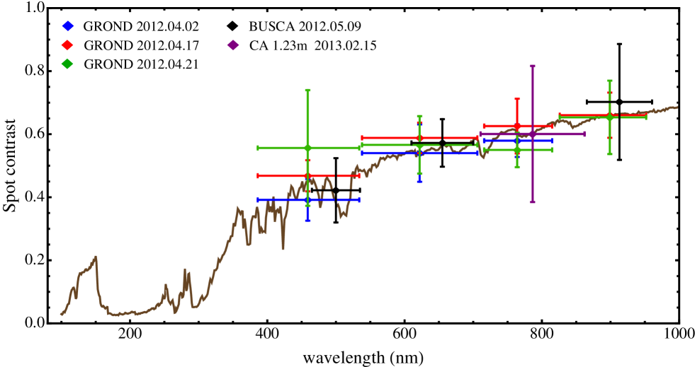
Figure 9: Variation of the spot contrast with wavelength. All the points are from this work and are explained in the upper-left legend. The vertical bars represent the errors in the measurements and the horizontal bars show the FWHM transmission of the passbands used. Solid line represents the spot-contrast variation expected for a starspot at 4200 K over a stellar photosphere of 4645 K.

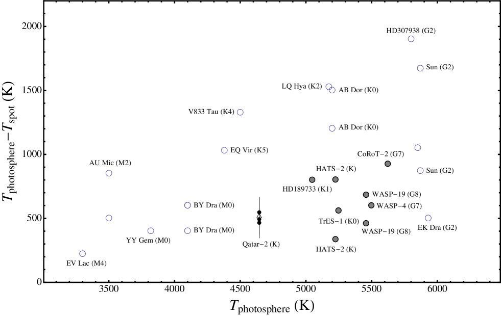
Figure 10: Spot temperature contrast with respect to the photospheric temperature in several dwarf stars taken from Berdyugina (2005), shown with empty circles. The name and spectral type of the star are also reported for most of them. The values for TrES-1, CoRoT-2, HD 189733, WASP-4, HATS-2, WASP-19 are taken from Rabus et al. (2009), Silva-Valio et al. (2010), Sing et al. (2011), Sanchis-Ojeda et al. (2011), Mohler-Fischer et al. (2013), Mancini et al. (2013c) and Huitson et al. (2013), respectively. Their positions in the diagram are marked with gray dots. The error bars have been suppressed for clarity. Note that some stars appear twice. The black dots and the triangle refer to the values estimated with GROND and BUSCA, respectively, for the case of Qatar-2 (this work).

Another type of precious information that we can obtain from follow-up transit observations comes from observing multiple planetary transits across the same starspot or starspot complex (Sanchis-Ojeda et al., 2011). In these cases, there is a good alignment between the stellar spin axis and planet’s orbital plane and, by measuring the shift in position of the starspot between the transit events, one can constrain the alignment between the orbital axis of the planet and the spin axis of the star with higher precision than with the measurement of the Rossiter-McLaughlin effect (e.g. Tregloan-Reed et al. 2013). On the other hand, if the starspots detected at each transit are different, then the latitude difference of the starspots is fully degenerate with the sky-projected spin-orbit angle $\lambda$.

According to the orbital period of the transiting planet, the same starspot can be observed after consecutive transits or after some orbital cycles, presuming that in the latter case the star performs one or more complete revolutions. Therefore, in general, the distance $D$ covered by the starspot in the time between two detections is

$$D=(n\times 2\pi R_{\mathrm{lat}})+d,$$ (1)

where $n$ is the number of revolutions completed by the star, $R_{\mathrm{lat}}$ is the scaled stellar radius for the latitude at which the starspot have been observed and $d$ is the arc length between the positions of two transits in which the starspot is detected.

In the present case, we observed three close transits of Qatar-2 b, with GROND (Fig. 6). The transits #1 and #2 were separated by twelve days (nine cycles), while transits #2 and #3 by four days (three cycles). Calculating the weighted means of the starspot positions among the four bands for each of the three transits, we estimate

$$(\theta,\phi)_{\#1} = (37.59^{\circ}\pm 1.75^{\circ},74.48^{\circ}\pm 2.14^{\circ})$$

$$(\theta,\phi)_{\#2} = (-30.24^{\circ}\pm 1.52^{\circ},69.41^{\circ}\pm 3.22^{\circ})$$

$$(\theta,\phi)_{\#3} = (4.22^{\circ}\pm 0.05^{\circ},72.16^{\circ}\pm 2.76^{\circ})$$

Could the starspots detected in the very close transits #2 and #3 be the same? We find that Qatar-2 A rotates unrealistically slowly for the case $n=0$, i.e. $v_{(72^{\circ})}=0.31$ km s^-1. For $n=1$ we get $v_{(72^{\circ})}=9.6$ km s^-1, accomplishing a complete revolution in $P_{\mathrm{rot}}=3.88\pm 0.07\,\mathrm{d}$ at a colatitude of $72^{\circ}$. For $n=2$ we have $v_{(72^{\circ})}=18.9$ km s^-1, and for $n>2$ the star would rotate even faster. The rotation period of Qatar-2 A at the equator, estimated from the sky-projected rotation rate and the stellar radius (Sanchis-Ojeda et al., 2011), is

$$P_{\mathrm{rot}}\approx\frac{2\pi R_{\mathrm{A}}}{v\sin{i_{\star}}}=(14.0\pm 2.5\,\mathrm{d})\sin{i_{\star}},$$ (3)

where $i_{\star}$ is the inclination of the stellar rotation axis with respect to the line of sight ($v\,\sin{i_{\star}}=2.8$ km s^-1; Bryan et al., 2012). From this we can exclude that the starspots detected in transits #2 and #3 are the same.

We now turn to the more promising transits #1 and #2. From Eq. 1 with $n=1$ we find $v_{(72^{\circ})}=3.28\pm 0.13$ km s^-1 which corresponds to $P_{\mathrm{rot}}=11.4\pm 0.5\,\mathrm{d}$. This is within $1\sigma$ of the equatorial value found above. Under the assumption that we have detected the same spot in these two transits, simple algebra gives the sky-projected angle between the stellar rotation and the planetary orbit to be $\lambda=4.3^{\circ}\pm 4.5^{\circ}$. This is the first measurement of the orbital obliquity of Qatar-2 and is consistent with orbital alignment ($\lambda=0$). This result is also in agreement with the general idea that cool stars have low obliquity (Winn et al., 2010).

The fact that we observed spot crossing events in every one of our high-precision transit light curves suggests that the host star has an active region underneath the transit cord. This idea was put forward by (Sanchis-Ojeda & Winn, 2011) for HAT-P-11, a rather different case where the planet’s orbital axis is inclined by nearly 90^∘ to the stellar rotational axis and the spot events cluster at two orbital phases in the transit light curve (see fig. 24 in Southworth, 2011).

7 Variation of the planetary radius with wavelength

As discussed in Sect. 2.3, simultaneous multi-band transit observations allow the chemical composition of the planet’s atmosphere to be probed in a way similar to transmission spectroscopy.

In Sect. 5 we estimated an equilibrium temperature of $1344\pm 14$ K for Qatar-2 b, which suggests, in the terminology of Fortney et al. (2008), that this planet should belong to the pL class. Therefore, based on the theoretical perspective of Fortney et al. (2008), it is not expected that the atmosphere of the planet should host a large amount of absorbing molecules, such as gaseous titanium oxide (TiO) and vanadium oxide (VO). By using the data reported in Table 4, we investigated the variations of the radius of Qatar-2 b in the wavelength ranges accessible to the instruments used, i.e. $386$–$976$ nm. In particular, we show in Fig. 11 the values of $k$ (the planet/star radius ratio) determined from the analysis of each transit separately versus wavelength. The vertical bars represent the relative errors in the measurements and the horizontal bars show the full-width at half-maximum (FWHM) transmission of the passbands used.

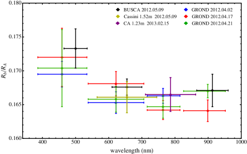
Figure 11: Variation of the planetary radius, in terms of the planet/star radius ratio, with wavelength. All the points are from this work and are explained in the upper-right legend. The vertical bars represent the errors in the measurements and the horizontal bars show the FWHM transmission of the passbands used.

The depths from the transit observations all agree with each other within $\sim$2$\sigma$, even if the $g$-band data indicate a larger value of $k$ at this wavelength region. As discussed in Sect. 4, this is likely caused by unocculted starspots which affect the measure of the transit depth in the bluest optical bands (see Fig. 8).

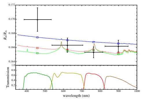
Figure 12: Variation of the planetary radius, in terms of planet/star radius ratio, with wavelength. The black points are the weighted-mean results coming from the three transit observations performed with GROND. The vertical bars represent the errors in the measurements and the horizontal bars show the FWHM transmission of the passbands used. The observational points are compared with three synthetic spectra at 1250 K, which do not include TiO and VO opacity. With respect to the model identified with the green line, the other two have H₂/He Rayleigh scattering increased by a factor of 10 (red dot line) and 1000 (blue dashed line). An offset is applied to all three models to provide the best fit to our radius measurements. Coloured squares represent band-averaged model radii over the bandpasses of the observations. Transmission curves of the GROND filters are shown in the bottom panel.

In order to have a more homogeneous set of data, we consider only the weighted-mean results coming from the three transit observations performed with GROND over 19 days. They are shown in Fig. 12 together with three one-dimensional model atmospheres developed by Fortney et al. (2010) for comparison. The green line has been calculated for Jupiter’s gravity (25 m s^-2) with a base radius of 1.25$\,{R}_{\rm Jup}$ at the 10 bar level and at 1250 K. The opacity of TiO and VO molecules is excluded from the model and the optical transmission spectrum is dominated by Rayleigh scattering in the blue, and pressure-broadened neutral atomic lines of sodium (Na) at 589 nm and potassium (K) at 770 nm. The other two models are equal but with H₂/He Rayleigh scattering increased by a factor of 10 (red dot line) and 1000 (blue dashed line). The GROND data clearly indicate a very large radius of Qatar-2 b in the wavelength range $400$–$510$ nm; the value of $R_{\mathrm{b}}$ measured in the $g^{\prime}$ band differs by $\sim 11670$ km from that in the $r^{\prime}$ band, which equates to $\sim 60\,H$, where $H$ is the atmospheric pressure scale height. A reasonable explanation for this nonphysical result is to advocate the presence of unocculted starspots which strongly contaminate the stellar flux in the $g^{\prime}$ band. Actually, if we correct the value of $k$ in the $g^{\prime}$ band by 0.0015 (cfr. Fig. 8), we obtain a planetary radius which is still large compared to the other bands, but straightforwardly explicable within the error bar by Rayleigh-scattering processes occurring in the atmosphere of Qatar-2 b (blue line in Fig. 12). A long photometric monitoring of Qatar-2 A is mandatory to estimate the right correction to make and new transit events observations in the $u$ or $U$ bands are also suggested in order to confirm the Rayleigh-scattering signature.

The lower value of the radius in the $i^{\prime}$ band could suggest a lack of K, even if the spectral resolution of GROND is not enough good to allow a clear determination. However, if true, this lack is attributable to a selective destruction process via photoionization, or its presence in a more condensed state. Another possible explanation is that the planet formed very far from the star, on the boundaries of the protoplanetary disk, before migrating to its current position.

8 Summary and conclusions

We have reported new broad-band photometric observations of five transit events in the Qatar-2 planetary system. Three of them were simultaneously monitored through four optical bands with GROND at the MPG/ESO 2.2-m telescope, and one through three optical bands with BUSCA at the CAHA 2.2-m telescope and contemporaneously with the Cassini 1.52-m telescope in one band. Another single-band observation was obtained at the CAHA 1.23-m telescope. In total we have collected 17 new light curves, all showing anomalies due to the occultation of starspots by the planet. These were fitted using the prism+gemc codes which are designed to model transits with starspot anomalies. Three further transits of Qatar-2 b were observed with a 25-cm telescope, and fitted with the jktebop code. Our principal results are as follows.

($i$) We used our new data and those collected from the discovery paper and web archives to improve the precision of the measured orbital ephemerides. We also investigated possible transit timing variations generated by a putative outer planet and affecting Qatar-2 b’s orbit. Unfortunately, the sampling of transit timings is not yet sufficient to detect any clear sinusoidal signal. A more prolonged monitoring of this system is mandatory in order to accurately characterise a possible TTV signal.

($ii$) We have revised the physical parameters of Qatar-2 b and its host star, significantly improving their accuracy. They are summarised in Table 7. In particular we find that density of Qatar-2 b is lower than the estimate by Bryan et al. (2012). The theoretical radius calculated by Fortney et al. (2007) for a core-free planet at age 4.5 Gyr and distance 0.02 AU is 1.17$\,{R}_{\rm Jup}$ for a planet of mass 2.44$\,{M}_{\rm Jup}$. These numbers are in good agreement with the parameters that we have estimated and imply that Qatar-2 b is coreless. Fig. 11 shows the new position of Qatar-2 b in the mass-radius diagram (left-hand panel) and in the plot of orbital period versus surface gravity (right-hand panel).

($iii$) The detection of so many starspots in our light curves suggests an intense period of activity for Qatar-2 A. The extent of each starspot was estimated and found to be in agreement with those found for similar starspot detections in other planetary systems during transit events. The projected positions ($\theta,\phi$) of each starspot was also determined, and the colatitudes were found to be consistent with $72^{\circ}$. For the four simultaneous multi-band observations, we detected a variation of the starspot contrast as a function of wavelength, as expected due to the different temperatures of starspots and the surrounding photosphere. The multi-colour data allowed a precise measurement of the temperature of each starspot. The values that we found are well in agreement with those found for other dwarf stars.

($iv$) The starspots detected in the GROND transits #1 and #2 present similar characteristics in terms of size, temperature and latitude, suggesting that we observed the same starspot in two transit events spaced by a time span during which Qatar-2 A performed one complete revolution. This allows a precise measurement of the rotation period of Qatar-2 A, $P_{\mathrm{rot}}=11.4\pm 0.5\,\mathrm{d}$ at a colatitude of $72^{\circ}$, and the sky-projected spin orbit alignment, $\lambda=4.3^{\circ}\pm 4.5^{\circ}$. The latter result implies that the orbital plane of Qatar-2 b is well aligned with the rotational axis of its parent star.

($v$) Thanks to the ability of GROND and BUSCA to measure stellar flux simultaneously through different filters, covering quite a large range of optical wavelengths, we were able to search for a radius variation of Qatar-2 b as a function of wavelength. All of the measurements are consistent with a larger value of the planet’s radius in the $g$-band when compared with the redder bands. This phenomenon is attributable to unocculted starspots which affect more strongly our measurements in the $g$ band. By focussing on the results coming from the three close transits observed with GROND, we reconstructed a more accurate transmission spectrum of the planet’s atmosphere in terms of the planet/star radius ratio and compared it with three synthetic spectra, based on model atmospheres in chemical equilibrium in which the presence of strong absorbers were excluded, but with differing amounts of Rayleigh scattering (Fig. 12). If we correct the $g^{\prime}$-band by the amount indicated by atmospheric models, the comparison between experimental data and synthetic spectra suggests that the atmosphere of Qatar-2 b could be dominated by Rayleigh scattering at bluer wavelengths. The low value of the radius observed between $700$ and $800$ nm should be explicable by a lack of potassium in the atmosphere of the planet (probably caused by star-planet photoionization processes). This hypothesis could be investigated with narrower-band filters.

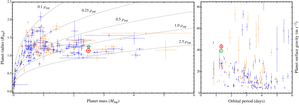
Figure 13: Left-hand panel: plot of the masses and radii of the known TEPs. The orange symbols denote values from the Homogeneous Studies project and the blue symbols results for the other known TEPs. Qatar-2 b is shown in red (Bryan et al., 2012) and green (this work). Dotted lines show where density is 2.5, 1.0, 0.5, 0.25 and 0.1 $\rho_{\mathrm{Jup}}$. Right-hand panel: plot of the orbital periods and surface gravities of the known TEPs. The symbols are the same as for left-hand panel. Data taken from Transiting Extrasolar Planet Catalogue, available at http://www.astro.keele.ac.uk/jkt/tepcat/ (Southworth, 2011).

Appendix A S/N estimations

In order to test the goodness of the measurements reported in this paper, we present signal-to-noise ratio (S/N) expectations for the simultaneous multi-band photometric observations of Qatar-2 with GROND. For each of the four GROND optical bands, we can quantify the ratio of noise-to-signal per unit time by

$$\rho=\sigma_{\mathrm{total}}\sqrt{t_{\mathrm{exp}}+d_{\mathrm{readout}}},$$ (4)

where $t_{\mathrm{exp}}$ is the exposure time and $d_{\mathrm{readout}}$ is the total dead time per observation – the latter quantity is generally dominated by the CCD readout time, but for GROND we have also to consider an extra dead time due to the synchronization of the optical observations with the NIR ones. $\sigma_{\mathrm{total}}$ is the total noise in a specific band for 1 mag measurement in one observation and takes into account five noise contributions that are added in quadrature. They are the Poisson noise from the target and background, readout noise, flat-fielding noise and scintillation, i.e.

$$\sigma_{\mathrm{total}}=\sqrt{\sigma_{\mathrm{target}}^{2}+\sigma_{\mathrm{sky}}^{2}+\sigma_{\mathrm{ron}}^{2}+\sigma_{\mathrm{flat}}^{2}+\sigma_{\mathrm{scint}}^{2}}.$$ (5)

Following the procedure described by Southworth et al. (2009), we performed S/N calculations for the GROND observations presented in this work. The count rates for the target (overall) and for the sky background (per pixel) were gathered from the SIGNAL code, scaling for the difference in telescope aperture and CCD plate scale. The magnitudes of Qatar-2 in Sloan $g$, $r$ and $i$ were taken from AAVSO archive. The magnitude in Sloan $z$ was obtained by interpolating the previous ones with $J$, $H$ and $K$ magnitudes taken from the NOMAD catalog (Zacharias et al., 2004). Other input parameters, specific for each band, were the readout noise of the CCD detector, the signal per pixel from the target averaged over the PSF, the maximum total count in a pixel (target plus sky) and the number of pixels inside the annulus of the target to apply flat-field noise. The resulting curves of noise level per observation are plotted in millimagnitudes as a function of $t_{\mathrm{exp}}$ in Fig. 14 for dark time and high observational cadence (solid curves) and for bright time and low cadence (dashed curves), cfr. Table 1.

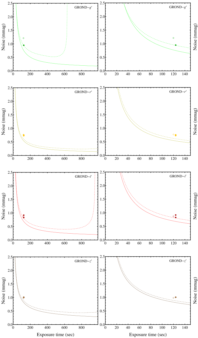
Figure 14: Predicted noise levels for the GROND observations presented in this work, but as a function of exposure time. The solid curves show the predicted noise level per observation for dark time and high observational cadence, whereas the dashed curves that per observation in bright time and low cadence. Panels in the left-hand column are for each of the four GROND optical bands. Panels in the right-hand column are the same of left-hand column, but zoomed to $t_{\mathrm{exp}}<150$. Diamonds represent the measurements of the two Qatar-2 b transits in dark time with a cadence of 150 s and empty diamonds are for the measurements of the transit in bright time with a cadence of 200 s (cfr. Table 1).

The scatter of our measurements are a bit higher than the expected noise, but fully consistent.

References

- Alonso et al. (2008) Alonso R., Barbieri M., Rabus M., Deeg H. J., Belmonte, J. A., Almenara J. M., 2008, A&A, 487, L5
- Ballerini et al. (2012) Ballerini P., Micela G., Lanza, A. F., Pagano I., 2012, A&A, 539, 140
- Bayliss et al. (2013) Bayliss D., et al., 2013, AJ, 146, 113
- Berdyugina (2005) Berdyugina S. V., 2005, Living Rev. Solar Phys., 2, 8
- Bento et al. (2013) Bento J., 2013, MNRAS in press
- Bryan et al. (2012) Bryan, M. L., et al., 2012, ApJ, 750, 84
- Bryan et al. (2014) Bryan, M. L., et al., 2014, ApJ, 782, 121
- Ciceri et al. (2013) Ciceri S., et al., 2013, A&A, 557, A30
- Claret (2000) Claret A., 2000, A&A, 363, 1081
- Claret (2004) Claret A., 2004, A&A, 428, 1001
- Copperwheat et al. (2013) Copperwheat C. M., et al., 2013, MNRAS, 434, 661
- de Mooij et al. (2012) de Mooij E. J. W., et al., 2012, A&A, 538, A46
- Désert (2011) Désert J.-M., et al., 2011, ApJS, 197, 14
- de Wit & Seager (2013) de Wit J., Seager S., 2013, Science, 342, 147
- Diaz-Cordoves et al. (1995) Diaz-Cordoves J., Claret A., Gimenez A., 1995, A&AS, 110, 329
- Enoch et al. (2010) Enoch B., Collier Cameron A., Parley N. R., Hebb L., 2010, A&A, 516, A33
- Fortney et al. (2007) Fortney J. J., Marley M. S., Barneset J. W., 2007, ApJ, 659, 1661
- Fortney et al. (2008) Fortney J. J., Lodders K., Marley M. S., Freedman R. S., 2008, ApJ, 678, 1419
- Fortney et al. (2010) Fortney J. J., Shabram M., Showman A. P., et al., 2010, ApJ, 709, 1396
- Gibson et al. (2008) Gibson N. P., Pollacco D., Simpson E. K., et al., 2008, A&A, 492, 603
- Gillon et al. (2006) Gillon M., Pont F., Moutou C., et al., 2006, A&A, 459, 249
- Greiner et al. (2008) Greiner J., et al., 2008, PASP, 120, 405
- Holman et al. (2010) Holman M. J., et al., 2010, Science, 330, 51
- Huitson et al. (2013) Huitson C. M., et al., 2013, MNRAS, 434, 3252
- Kurucz (1979) Kurucz R. L., 2013, ApJS, 40, 1
- Lendl et al. (2013) Lendl M., Gillon M., Queloz D., Alonso R., Fumel A., Jehin E., Naef D., 2013, A&A, 552, A2
- Maciejewski et al. (2013) Maciejewski G., et al., 2013, A&A, 551, A108
- Mancini et al. (2013a) Mancini L., et al., 2013a, A&A, 551, A11
- Mancini et al. (2013b) Mancini L., et al., 2013b, MNRAS, 430, 2932
- Mancini et al. (2013c) Mancini L., et al., 2013c, MNRAS, 436, 2
- Mancini et al. (2014) Mancini L., et al., 2014, A&A, 562, A126
- Mohler-Fischer et al. (2013) Mohler-Fischer M., et al., 2013, A&A, 558, A55
- Narita et al. (2013) Narita N., et al., 2013, ApJ, 773, 144
- Nesvorný et al. (2013) Nesvorný D., Kipping D. M., Buchhave L. A., Bakos G. Á., Hartman J., Schmitt A. R., 2012, Science, 336, 1133
- Nikolov et al. (2013) Nikolov, N., Chen, G., Fortney, J. J., Mancini L., Southworth J., van Boekel R., Henning Th., 2013, A&A, 553, A26
- Penev et al. (2013) Penev K., et al., 2013, AJ, 145, 5
- Pierini et al. (2012) Pierini D., et al., 2012, A&A, 540, A45
- Pont et al. (2007) Pont F., et al., 2007, A&A, 476, 1347
- Pont et al. (2013) Pont F., Sing D. K. Gibson, N. P. Aigrain S., Henry G., Husnoo N., 2013, MNRAS, 432, 2917
- Rabus et al. (2009) Rabus M., et al., 2009, A&A, 494, 391
- Rothery et al. (2011) Rothery D. A., McBride N., Gilmour I., 2011, An Introduction to the Solar System (Cambidge University Press)
- Sanchis-Ojeda et al. (2011) Sanchis-Ojeda R., Winn J. N., Holman M. J., 2011, ApJ, 733, 127
- Sanchis-Ojeda & Winn (2011) Sanchis-Ojeda R., Winn J. N., 2011, ApJ, 743, 61
- Seager & Mallén-Ornelas (2003) Seager S., Mallén-Ornelas G., 2003, ApJ, 585, 1038
- Silva (2003) Silva A. V. R., 2003, ApJL, 585, L147
- Silva-Valio et al. (2010) Silva-Valio A., Lanza A. F., Alonso R., Barge P. 2010, A&A, 510, A25
- Sing et al. (2011) Sing D. K., et al., 2011, MNRAS, 416, 1443
- Seager & Mallén-Ornelas (2003) Seager S., & Mallén-Ornelas G., 2003, ApJ, 585, 1038
- Southworth (2011) Southworth J., 2011, MNRAS, 417, 2166
- Southworth (2012) Southworth J., 2012, MNRAS, 426, 1291
- Southworth et al. (2009) Southworth J., et al., 2009, MNRAS, 396, 1023
- Southworth et al. (2010) Southworth J., et al., 2010, MNRAS, 408, 1680
- Southworth et al. (2011) Southworth J., et al., 2011, A&A, 527, A8
- Southworth et al. (2012a) Southworth J., Bruni I., Mancini L., Gregorio J., 2012a, MNRAS, 420, 2580
- Southworth et al. (2012b) Southworth J., et al., 2012b, MNRAS, 422, 3099
- Southworth et al. (2012c) Southworth J., et al., 2012c, MNRAS, 426, 1338
- Southworth et al. (2013) Southworth J., et al., 2013, MNRAS, 434, 1300
- Strassmeier (2009) Strassmeier K. G., 2009, Astron. Astrophys. Rev., 17, 251
- Tregloan-Reed et al. (2013) Tregloan-Reed J., Southworth J., Tappert C., 2013, MNRAS, 428, 3671
- van Hamme (1993) van Hamme W., 1993, AJ, 106, 2096
- Winn et al. (2008) Winn J. N., et al., 2008, ApJ, 683, 1076
- Winn et al. (2010) Winn J. N., Fabrycky D., Albrecht S., Johnson J. A., 2010, ApJ, 718, L145
- Zacharias et al. (2004) Zacharias N., Monet D. G., Levine, S. E., Urban S. E., Gaume R., Wycoff G. L., 2004, American Astron. Soc. meeting, 205, #48.15