Snow-lines as probes of turbulent diffusion in protoplanetary discs
Abstract
Sharp chemical discontinuities can occur in protoplanetary discs, particularly at ‘snow-lines’ where a gas-phase species freezes out to form ice grains. Such sharp discontinuities will diffuse out due to the turbulence suspected to drive angular momentum transport in accretion discs. We demonstrate that the concentration gradient - in the vicinity of the snow-line - of a species present outside a snow-line but destroyed inside is strongly sensitive to the level of turbulent diffusion (provided the chemical and transport time-scales are decoupled) and provides a direct measurement of the radial ‘Schmidt number’ (the ratio of the angular momentum transport to radial turbulent diffusion). Taking as an example the tracer species N2H+, which is expected to be destroyed inside the CO snow-line (as recently observed in TW Hya) we show that ALMA observations possess significant angular resolution to constrain the Schmidt number. Since different turbulent driving mechanisms predict different Schmidt numbers, a direct measurement of the Schmidt number in accretion discs would allow inferences about the nature of the turbulence to be made.
Subject headings:
accretion, accretion disks - protoplanetary disks - turbulence - astrochemistry1. Introduction
Astrophysical discs are observed to transport angular momentum. It has been hypothesised that such discs are transporting angular momentum through a turbulent process (Shakura & Sunyaev, 1973). Despite decades of theoretical research we still lack a sufficient understanding of turbulence to make quantitative predictions. Several candidate processes exist to sustain turbulence in these discs: the magneto-rotational instability (MRI) (e.g. Balbus & Hawley, 1991), gravitational instability (e.g. Lodato & Rice 2004, 2005) the vertical shear instability (Nelson et al., 2013) and the baroclinc instability (e.g. Klahr & Bodenheimer, 2003). The MRI is still the leading candidate for angular momentum transport in accretion discs (see Turner et al. 2014 for a recent review). However, at the low temperatures and ionization fractions expected in protoplanetary discs, non-ideal MHD effects become important, qualitatively changing the nature of the turbulence and its associated transport properties, or rendering it ineffective resulting in ‘dead-zones’ (e.g. Gammie, 1996).
A corollary to the angular momentum transport problem in protoplanetary discs is the transport of dust particles. There is large amounts of astrophysical (e.g Bouwman et al., 2001; Dullemond et al., 2006; Hughes & Armitage, 2010; Owen et al., 2011b) and cosmochemical (e.g Gail, 2001; Bockelée-Morvan et al., 2002; Jacquet et al., 2012; Jacquet & Robert, 2013) evidence to suggest large scale radial transport of dust particles occurs. In particular, the level of diffusion that results from the turbulence is an unknown parameter. The turbulent diffusion coefficient () is often parametrised in terms of the turbulent kinematic viscosity () as where is the Schmidt number. Assumptions of isotropic, Kolmogorov-like turbulence lead to the inference that (Youdin & Lithwick, 2007); however, a large range of reported experimental/theoretical/numerical values exist that span approximately two orders of magnitude in the range (Prinn, 1990; Dubrulle & Frisch, 1991; Lathrop et al., 1992; Carballido et al., 2005; Johansen et al., 2006; Youdin & Lithwick, 2007; Zhu et al., 2014).
Direct observational measurements of the strength of turbulent diffusion in the continuum will be complicated by dust-drag, grain growth/fragmentation and optical depth effects. However, it is not only dust particles that will experience turbulent diffusion; any rare, gas-phase species (tracer species) where changes in temperature results in a concentration gradient will also experience turbulent diffusion. If, for example, a tracer species is predominately produced at a given radius, the tracer will then diffuse away from this radius, with a distribution that is strongly dependent on the value of the Schmidt number (Clarke & Pringle, 1988). Jacquet & Robert (2013) considered the case of deuterated water and argued the D/H water distribution in Chondrites implies the Schmidt number is smaller than unity.
Snow-lines, where a gas phase tracer (for example H2O, CO2, CO) condenses out of the gas to form ice below some temperature represents a scenario where a sharp concentration gradient can occur. Species such as H2O, CO2 & CO are relatively abundant, such that the surface layers can be optically thick. Additionally, model degeneracies make it difficult to constrain snow-lines directly (even with optically thin isotopologues). However, if the production/destruction of yet rarer tracers are regulated by the presence or absence of gas phase H2O, CO2 or CO then these rare tracers could be used as proxies to detect snow-lines. For the CO snow-line it is expected that N2H+ and H2CO will only be abundant when CO freezes out (Jørgensen et al., 2004; Walsh et al., 2012; Qi et al., 2013a, b). Such an expectation has been born out in observations of star-forming cores (Friesen et al., 2010), and similar results were obtained in the DISCS SMA survey of several nearby protoplanetary discs (Qi et al., 2013a). Recently, Qi et al. (2013b) imaged a hole in N2H+ using ALMA at a radius of AU, co-incident with the expected location of the CO snow-line (based on a free-out temperature of K). The sharpness of the inner edge will depend strongly on the strength of the turbulent diffusion, with weaker diffusion resulting in a sharper hole.
In this letter we demonstrate how the distribution of a tracer species that is only abundant outside a snow-line (being destroyed inside) is strongly dependant on the Schmidt number, and that ALMA observations could be able to constrain the Schmidt number in protoplanetary discs.
2. Disc Model
We consider a 1D axis-symmetric disc, where the evolution of the gas surface density () and the surface density of any (gas-phase) tracer species () is given by (e.g. Lynden-Bell & Pringle, 1974; Clarke & Pringle, 1988; Birnstiel et al., 2010; Owen et al., 2011a; Owen, 2014):
| (1) | |||||
| (2) | |||||
where is the concentration of the tracer species, is the net radial gas velocity, is the radial gas turbulent diffusion co-efficient and is a source/sink term that represents the production and destruction of the tracer species.
2.1. Conditions at the snow-line
The following general model can be applied to any snow-line (H2O, CO2, CO, etc.) where the chemical and transport time-scales decouple. Here we specifically consider the case of N2H+ destruction at the CO snow-line as observed in TW Hya (Qi et al., 2013b). Inside the CO snow-line N2H+ is destroyed by gas phase CO, outside the CO snow line this destruction channel is no-longer dominant and it instead is destroyed at a much slower rate by dissociative recombination (Jørgensen et al., 2004). Simulations without transport suggest the N2H+ abundance drops by several orders of magnitude inside the CO snow-line (e.g. Walsh et al., 2012) with an abundance that depends on the square of the gas-phase CO abundance (Jørgensen et al., 2004).
2.1.1 Relevant Time-scales
In order for chemical tracers at the snow-line to be useful in terms of probing the strength of the turbulent diffusion, we must de-couple the chemical and dynamical time-scales. Namely, the desorption time-scale must be faster than the transport time-scales in-order to create a sharp snow-line; furthermore, the destruction time-scale of the tracer species inside the snow-line must also be fast. The transport time-scales of interest are the time with which to move a radial distance (where is the disc’s scale height111We note since the snow-line is sharp, the relevant length scale for computing time-scales is , not . which is of order the radial scale length). Therefore, the advection time-scale () is:
| (3) | |||||
and the diffusive time-scale () is:
| (4) |
It is well known (e.g. Clarke & Pringle, 1988; Jacquet et al., 2012; Jacquet & Robert, 2013)222We will derive this dependence in Section 2.2 for a steady disc model, but it is a more general result - see Clarke & Pringle (1988). the logarithmic concentration gradient rapidly approaches , thus the diffusive time-scale is identical to the advection time-scale (this is somewhat unsurprising as they are both driven by the same process). Thus, the relevant time-scale for the movement of a individual tracer molecule over a radial scale is () years.
We want to compare this transport time-scale to the time-scale for the desorption of the snow-line species, along with the destruction of the tracer species inside the snow-line. Considering our example of N2H+ and the CO snow-line then the desorption time-scale is obtained by balancing desorption with absorption (with rate constant ), so the desorption time-scale becomes (Takahashi & Williams, 2000):
| (5) | |||||
where is the dust-grain size, is the dust-to-gas mass ratio and is the CO abundance. Additionally, the destruction time-scale for N2H+ is (from the Jørgensen et al. 2004 simplified network):
| (6) | |||||
where is the destruction rate constant333Estimated from Figure 16 of Jørgensen et al. (2004)..
Therefore, the CO/N2H+ system clearly satisfies , for conditions experienced in protoplanetary discs. As such we may ignore the details of the chemical rate equations and simply model the destruction of any remaining N2H+ to occur instantaneously at the snow-line radius; although, we emphasise that the following analysis can be applied to any tracer species with similar destruction time-scales. Therefore, in this situation the source function is drastically simplified to:
| (7) |
where is the mass-accretion rate, is the concentration at large radius, is the Dirac delta-function and is the radius of the snow-line. This source function represents the instantaneous destruction of any remaining tracer species at . We note it ignores any possible vertical structure of the snow-line, which will necessarily spread out the destruction region of the tracer species (Walsh et al., 2012) and we discuss the implications of this caveat in Section 4.
2.2. Steady-disc models
We will now restrict ourselves to a steady disc problem. In that case Equation 1 becomes : where is the accretion rate, and we have neglected the very small contribution due to an inner boundary at finite radius. Furthermore, the equation for the gas tracer becomes:
| (8) |
where is the radial Schmidt number. Therefore, radially integrating Equation 8 and using our expression for we find:
| (9) |
Using Equation 7 we can integrate Equation 9 to find the radial concentration distribution:
| (10) |
where is the Heaviside step function. Setting at we find the solution:
| (11) |
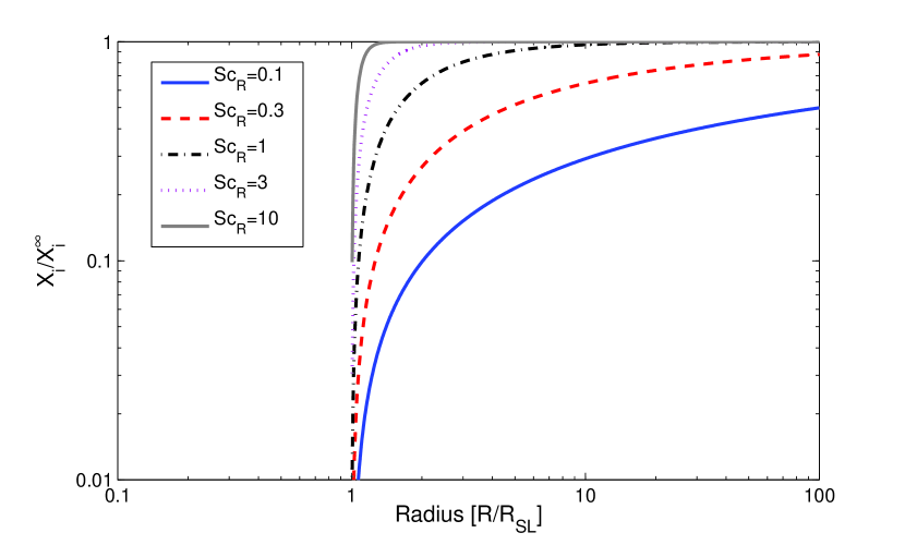
Therefore, we see that the radial profile of the concentration is strongly sensitive to the value of the Schmidt number. In Figure 1 we show how the concentration varies with radius and Schmidt number. It is important to emphasise that concentration distribution is independent of assumptions of the (unknown) viscosity, and mass-accretion rate and can in principle provide a ‘clean’ measurement of the Schmidt number.
3. Observable characteristics
Unfortunately it is not possible to directly observe the concentration gradient. What is directly observed is the surface-brightness distribution of the relevant species. The surface-brightness distribution is sensitive to the surface density of the tracer species rather than its concentration. Thus, we must multiply the concentration of our tracer species by the gas surface density. Adopting a power-law gas distribution of the form with a cut-off radius , the surface density of the tracer species is:
| (12) |
in the range and elsewhere.
3.1. Brightness distribution and Visibility profiles
The actual brightness distribution from rotational emission lines (such as N2H+ J=4-3), as well as being sensitive to the surface density distribution is also sensitive to the background gas temperature and excitation temperature of the molecule (which in turn is a function of density and temperature) along with the optical depth.
However, in the case that the tracer species is optically thin, and the gas density is far above the critical density () for the rotational transition, then the molecular line is thermalised. Thus, if the temperature gradient is weak compared to the scales of interest and then we can approximate the surface brightness as being directly proportional to the surface density of the tracer species, provided the line remains optically thin.
For the gas at 30 AU the gas density is typically:
| (13) | |||||
where is the mean molecular weight of the gas. Comparing this to the critical density of the transition of N2H+ which has a critical density of cm-3 (e.g. Friesen et al., 2010), we see that . We note, since temperature and density are expected to be power-laws with radius (e.g. Chiang & Goldreich, 1997; Hartmann et al., 1998) then the small additional corrections due to temperature and density effects of converting to the surface brightness distribution () will manifest themselves as changes in the power-law index in Equation 14.
Assuming the disc to be axis-symmetric and observed face-on, we may write the brightness distribution on the sky as:
| (14) |
in the range and elsewhere, where is a constant, is the angular size on the sky and is the angular size of the snow-line given by:
| (15) |
Thus, we see that the brightness distribution still retains the strong sensitivity to the Schmidt number. Since the angular resolution required to probe the value of the Schmidt number is only available through mm-interferometry, we can use our brightness distribution to calculate synthetic visibilities. The visibilities can obtained by a Hankel transform of the axis-symmetric brightness-distribution such that:
| (16) |
where is a radial baseline co-ordinate defined as where & are the usual baseline co-ordinates. Following the observed N2H+ emission by Qi et al. (2013b) we calculate our synthetic observations at 372Ghz with our standard model adopting the best fit parameters from Qi et al. (2013b) of AU, AU and .
We calculate our synthetic observations assuming the source is observed face-on at a distance of 150pc. In Figure 2 we show our simulated visibility curves in the left-hand panels and the surface density profiles in the right hand panel. In the top panels we vary the Schmidt number between 0.1-10, in the middle panels we vary from 1-3 and in the bottom panels we vary from 15-60 AU.
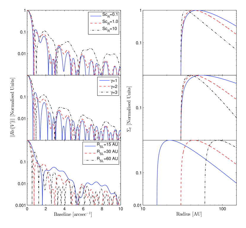
The visibility curves in Figure 2 clearly show that variations in the Schmidt number give rise to significant differences. Furthermore, comparisons between varying the index of the gas surface density , snow-line radius and the Schmidt number are not too degenerate. The simplified model presented here contains four free parameters , which would all need to be constrained by fitting the visibilities. Inspection of Figure 2 suggests that sensitivities % at base-lines km would allow the theoretically suggested range of Schmidt numbers (0.1-10) to be observationally constrained.
4. Discussion
We have shown that observations of snow-lines in protoplanetary discs using a tracer species (for example N2H+ in the case of the CO snow line Qi et al. 2013a, b) can be used to probe the Schmidt number, a unknown parameter in studies of turbulent transport in accretion discs, where current estimates span a range of two-orders of magnitude ( 0.1-10).
4.1. Detectability with ALMA
The ALMA telescope is a sub-mm/mm interferometer; once completed it will have individual antennas, offering baselines with separations upto 12 km. At 372 Ghz ( N2H+ J=4-3 line) this provides a maximum spatial resolution of arcsec. Figure 2 clearly shows that ALMA posses the required number of base-lines () with separations in the range 0.1-1 Km to constrain Schmidt values within the current range of uncertainty, provided the observations are sensitive enough. Taking the TW Hya N2H+ observations as reference (Qi et al., 2013b) - a source brightness mJy beam-1 km s-1 with an rms noise of 8.1 mJy beam-1 km s-1 and beam size arcsec made using 23-26 antennas444Since the beam size of the current TW Hya observation posses a resolution similar to then using the current observation to constrain the Schmidt number seems unlikely; however, using the velocity channels separately can be used to increase the effective resolution (e.g. Qi et al., 2013a). - a similar level of sensitivity, but with a beam size of arcsec, could be obtained assuming a fully operational ALMA of 50 antennas. Thus, such observations are feasible and sufficiently high resolution to allow constraints to be placed on the Schmidt number at the distance to TW Hya. Longer integration times and larger base-lines would be required to reach similar levels of sensitivity at distances of 150pc.
4.2. Uncovering properties of the turbulence
We have argued that the sharpness of the hole in tracer species at the snow-line probes the value of the Schmidt number independent of the assumed properties of the turbulence (e.g. assumed value of the viscous ‘’ parameter). Since several snow-lines are expected to occur at different radii, then measurements at different snow-lines would allow the radial dependence of the Schmidt number to be probed. In particular, recent simulation suggest that different non-ideal MHD effects (which dominate at different radii Turner et al. 2014) lead to different Schmidt numbers (Zhu et al., 2014). Thus, comparing the simulation predictions of the Schmidt number for various turbulent driving mechanisms with the observed value would allow inferences about the nature of the turbulence to be made.
Furthermore, independently measuring the rms turbulent velocity () (e.g. Hughes et al., 2011) then combining it with a measurement of the Schmidt number would allow the viscosity (including estimates of ) to be calculated, since .
4.3. Caveats & Limitations
We have constructed an idealised model to investigate whether snow-lines could begin to probe the strength of turbulent diffusion. As such there are several model improvements that must be made before fitting to real data. Therefore, our model presented in this letter is a ‘proof-of-concept’ rather than a road map for observational modelling. For example, a real protoplanetary disc is not one-dimensional. As such the vertical temperature structure is not constant and passively heated discs cool as one approaches the mid-plane (Chiang & Goldreich, 1997). Therefore, the snow-line is unlikely to occur exactly at a fixed radius, but is more-likely to be an extended structure with a scale variation of , with is time-varying position (Martin & Livio, 2012, 2013, 2014). Additionally the conversion of the gas phase to ice particles at the snow-line will result in turbulent diffusion of the gas and ice particles away from the snow-line (in identical manner to that discussed for the snow-line tracer discussed here). As such, there is unlikely to be a very sharp change in the gas abundance at the snow-line but rather a smoother change. Furthermore, the chemical time-scales may not fully decouple from the transport time-scales. In the N2H+ case considered here we have argued that the time-scales are likely to be decoupled; this may not be the case for all snow-line tracer species, thus dynamical modelling which includes turbulent diffusion is needed to determine the importance of this effect. The model presented here should provide a stringent upper limit of the Schmidt number, and good measurement if it is small (); however, if it is large, and the sharpness of the passive tracer has width of , then the 1D model would only provide an order of magnitude estimate and a better model is need to constrain the Schmidt number. Finally, if the snow-line resides in a dead-zone, where there is limited or no turbulence then it is unlikely this method can be used to cleanly probe the Schmidt number; but, dead-zones are not expected at the large radius of the CO/N2H+ system discussed here.
5. Summary
In this letter we have shown that the recent observations of snow-lines through tracer species (e.g. N2H+ or H2CO in the case of the CO snow-line Qi et al. 2013a, b) could allow direct observational measurements of the Schmidt number in astrophysical accretion discs. In the case that the chemical time-scale is suitably de-coupled from the transport time-scales then the concentration gradient of the tracer outside the snow-line directly depends on the Schmidt number in a power-law fashion () independent of the choice of the turbulent parameter.
We argue that the effect of turbulent diffusion on surface brightness distribution of such a snow line tracer is detectable with ALMA observations of discs in nearby star-forming regions which can possess high enough angular resolution to constrain the current theoretically/numerically estimated values of the Schmidt number ().
Observations of different snow-lines (e.g. H2O, CO2 & CO) at different radii in the discs would allow the radial dependence of the Schmidt number to be probed. Coupling these snow-line observations with observational estimates of the gas-surface density and turbulent line-widths would allow direct estimates of the strength and nature of the turbulence in astrophysical accretion discs.
References
- Balbus & Hawley (1991) Balbus, S. A., & Hawley, J. F. 1991, ApJ, 376, 214
- Birnstiel et al. (2010) Birnstiel, T., Dullemond, C. P., & Brauer, F. 2010, A&A, 513, A79
- Bockelée-Morvan et al. (2002) Bockelée-Morvan, D., Gautier, D., Hersant, F., Huré, J.-M., & Robert, F. 2002, A&A, 384, 1107
- Bouwman et al. (2001) Bouwman, J., Meeus, G., de Koter, A., et al. 2001, A&A, 375, 950
- Carballido et al. (2005) Carballido, A., Stone, J. M., & Pringle, J. E. 2005, MNRAS, 358, 1055
- Chiang & Goldreich (1997) Chiang, E. I., & Goldreich, P. 1997, ApJ, 490, 368
- Clarke & Pringle (1988) Clarke, C. J., & Pringle, J. E. 1988, MNRAS, 235, 365
- Dubrulle & Frisch (1991) Dubrulle, B., & Frisch, U. 1991, Phys. Rev. A, 43, 5355
- Dullemond et al. (2006) Dullemond, C. P., Apai, D., & Walch, S. 2006, ApJ, 640, L67
- Friesen et al. (2010) Friesen, R. K., Di Francesco, J., Shimajiri, Y., & Takakuwa, S. 2010, ApJ, 708, 1002
- Gail (2001) Gail, H.-P. 2001, A&A, 378, 192
- Gammie (1996) Gammie, C. F. 1996, ApJ, 457, 355
- Hartmann et al. (1998) Hartmann, L., Calvet, N., Gullbring, E., & D’Alessio, P. 1998, ApJ, 495, 385
- Hughes & Armitage (2010) Hughes, A. L. H., & Armitage, P. J. 2010, ApJ, 719, 1633
- Hughes et al. (2011) Hughes, A. M., Wilner, D. J., Andrews, S. M., Qi, C., & Hogerheijde, M. R. 2011, ApJ, 727, 85
- Jacquet et al. (2012) Jacquet, E., Gounelle, M., & Fromang, S. 2012, Icarus, 220, 162
- Jacquet & Robert (2013) Jacquet, E., & Robert, F. 2013, Icarus, 223, 722
- Johansen et al. (2006) Johansen, A., Klahr, H., & Mee, A. J. 2006, MNRAS, 370, L71
- Jørgensen et al. (2004) Jørgensen, J. K., Schöier, F. L., & van Dishoeck, E. F. 2004, A&A, 416, 603
- Klahr & Bodenheimer (2003) Klahr, H. H., & Bodenheimer, P. 2003, ApJ, 582, 869
- Lathrop et al. (1992) Lathrop, D. P., Fineberg, J., & Swinney, H. L. 1992, Phys. Rev. A, 46, 6390
- Lodato & Rice (2004) Lodato, G., & Rice, W. K. M. 2004, MNRAS, 351, 630
- Lodato & Rice (2005) Lodato G., Rice W. K. M., 2005, MNRAS, 358, 1489
- Lynden-Bell & Pringle (1974) Lynden-Bell, D., & Pringle, J. E. 1974, MNRAS, 168, 603
- Martin & Livio (2012) Martin, R. G., & Livio, M. 2012, MNRAS, 425, L6
- Martin & Livio (2013) —. 2013, MNRAS, 434, 633
- Martin & Livio (2014) —. 2014, ApJ, 783, L28
- Nelson et al. (2013) Nelson, R. P., Gressel, O., & Umurhan, O. M. 2013, MNRAS, 435, 2610
- Owen (2014) Owen, J. E. 2014, ApJ, 789, 59
- Owen et al. (2011a) Owen, J. E., Ercolano, B., & Clarke, C. J. 2011a, MNRAS, 412, 13
- Owen et al. (2011b) —. 2011b, MNRAS, 411, 1104
- Prinn (1990) Prinn, R. G. 1990, ApJ, 348, 725
- Qi et al. (2013a) Qi, C., Öberg, K. I., & Wilner, D. J. 2013a, ApJ, 765, 34
- Qi et al. (2013b) Qi, C., Öberg, K. I., Wilner, D. J., et al. 2013b, Science, 341, 630
- Shakura & Sunyaev (1973) Shakura, N. I., & Sunyaev, R. A. 1973, A&A, 24
- Takahashi & Williams (2000) Takahashi, J. & Williams, D. A. 2000, MNRAS, 314, 273
- Turner et al. (2014) Turner, N. J., Fromang, S., Gammie, C., et al. 2014, Protostars and Planets VI
- Walsh et al. (2012) Walsh, C., Nomura, H., Millar, T. J., & Aikawa, Y. 2012, ApJ, 747, 114
- Youdin & Lithwick (2007) Youdin, A. N., & Lithwick, Y. 2007, Icarus, 192, 588
- Zhu et al. (2014) Zhu, Z., Stone, J. M., & Bai, X.-N. 2014, ArXiv e-prints, arXiv:1405.2778