Homogeneous Photometry VI: Variable Stars in the Leo I Dwarf Spheroidal Galaxy^∗

Abstract

From archival ground-based images of the Leo I dwarf spheroidal galaxy we have identified and characterized the pulsation properties of 164 candidate RR Lyrae variables and 55 candidate Anomalous and/or short-period Cepheids. We have also identified nineteen candidate long-period variable stars and thirteen other candidate variables whose physical nature is unclear, but due to the limitations of our observational material we are unable to estimate reliable periods for them. On the basis of its RR Lyrae star population Leo I is confirmed to be an Oosterhoff-intermediate type galaxy, like several other dwarf spheroidals. From the RR Lyrae stars we have derived a range of possible distance moduli for Leo I: $22.06\pm 0.08\;\lower 2.58334pt\hbox{$\sim$}\kern-9.2pt\raise 1.72218pt\hbox{$<$}\;\mu_{0}\;\lower 2.58334pt\hbox{$\sim$}\kern-9.2pt\raise 1.72218pt\hbox{$<$}\;22.25\pm 0.07\,$mag depending on the metallicity assumed for the old population ([Fe/H] from –1.43 to –2.15). This is in agreement with previous independent estimates. We show that in their pulsation properties, the RR Lyrae stars—representing the oldest stellar population in the galaxy—are not significantly different from those of five other nearby, isolated dwarf spheroidal galaxies. A similar result is obtained when comparing them to RR Lyrae stars in recently discovered ultra-faint dwarf galaxies. We are able to compare the period distributions and period-amplitude relations for a statistically significant sample of ab–type RR Lyrae stars in dwarf galaxies ($\sim\,$1300 stars) with those in the Galactic halo field ($\sim\,$14,000 stars) and globular clusters ($\sim\,$1000 stars). Field RRLs show a significant change in their period distribution when moving from the inner ($d_{G}\;\lower 2.58334pt\hbox{$\sim$}\kern-9.2pt\raise 1.72218pt\hbox{$<$}\;\,$14 kpc) to the outer ($d_{G}\;\lower 2.58334pt\hbox{$\sim$}\kern-9.5pt\raise 1.72218pt\hbox{$>$}\;\,$14 kpc) halo regions. This suggests that the halo formed from (at least) two dissimilar progenitors or types of progenitor. Considered together, the RR Lyrae stars in classical dwarf spheroidal and ultra-faint dwarf galaxies—as observed today—do not appear to follow the well defined pulsation properties shown by those in either the inner or the outer Galactic halo, nor do they have the same properties as RR Lyraes in globular clusters. In particular, the samples of fundamental-mode RR Lyrae stars in dwarf galaxies seem to lack High Amplitudes and Short Periods (“HASP”: $A_{V}\geq 1.0\,$mag and P  $\sim$$<$  0.48 d) when compared with those observed in the Galactic halo field and globular clusters. The observed properties of RR Lyrae stars do not support the idea that currently existing classical dwarf spheroidal and ultra-faint dwarf galaxies are surviving representative examples of the original building blocks of the Galactic halo.

^∗Based in part on data obtained through the facilities of the Canadian Astronomy Data Centre operated by the National Research Council of Canada with the support of the Canadian Space Agency; data obtained from the ESO Science Archive Facility under muliple requests by the authors; data obtained from the Isaac Newton Group Archive, which is maintained as part of the CASU Astronomical Data Centre at the Institute of Astronomy, Cambridge; and data distributed by the NOAO Science Archive. NOAO is operated by the Association of Universities for Research in Astronomy (AURA) under cooperative agreement with the National Science Foundation.

1 Introduction

The nearby dwarf spheroidal galaxies (dSphs, L $\sim$$>$ 10⁵L_⊙) are important for understanding the formation and evolution of the Milky Way Galaxy. Their very old ages ( $\sim$$>$ 10 Gyr) and low mean metallicities ([Fe/H] $\sim$$<$ –1.3 dex) have long been used as evidence for the idea that these systems are fossils from the early Universe: surviving examples of the pre-galactic units that formed the Galactic stellar halo, as predicted by hierarchical models of galaxy formation (see White & Frenk 1991; Salvadori & Ferrara 2009, and references therein). This view has been widely held for at least the last twenty years, since detailed stellar population studies have been made possible by new deep color-magnitude diagrams (CMDs) and medium- and high-resolution spectroscopic analyses (Mateo 1998; Tolstoy et al. 2009). Today, we have at our disposal accurate star-formation histories (Tolstoy & Saha 1996; Gallart et al. 1999; Cole et al. 2007; Monelli et al. 2010a, b; Hidalgo et al. 2011; de Boer et al. 2012a, b) and chemical abundance distributions (Venn et al. 2004; Kirby et al. 2009, 2011; Fabrizio et al. 2012; Lemasle et al. 2012; Kirby et al. 2013) for a large number of nearby dSphs and dwarf irregulars (dIs). However, high-resolution spectroscopy has shown that the [$\alpha$/Fe] abundance patterns of stars in dSphs do not seem to resemble those of Galactic halo stars (Shetrone et al. 2001; Venn et al. 2004; Pritzl et al. 2005). This could pose some problems for their identification as representative building blocks of the halo. On the other hand, it could also be explained by the fact that present-day dSphs, having not accreted at early epochs, have had a Hubble time to evolve as independent entities under conditions that are different in a variety of ways from those experienced by field halo stars. In support of this interpretation, Font et al. (2006) have argued that differences in the chemical abundances of the Galactic halo and its satellites can be explained within their hierarchical formation model of the halo, which carefully tracks the orbital evolution and tidal disruption of its satellites.

A new source of puzzlement was raised by Helmi et al. (2006), who obtained large samples of low- and intermediate-resolution spectra of red giant branch (RGB) stars of the Sculptor, Sextans, Fornax, and Carina dSph galaxies as part of a huge observational effort devoted to the characterization of the chemical abundances of those systems (see Tolstoy et al. 2006, and references therein). For the first time, Helmi et al. (2006) noticed a significant lack of extremely metal-poor stars ([Fe/H] $\sim$$<$ –3 dex) in the galaxies’ metallicity distributions when compared with that of the Galactic halo. The most metal-poor stars in a galaxy are likely to be also the oldest ones so—taken at face value—this evidence again seems to argue against the idea that nearby dSphs are surviving examples of the main contributors to the Milky Way halo. In order to further investigate this issue, Starkenburg et al. (2010) revisited the calibration of [Fe/H] as inferred from the observed strength of the infrared calcium triplet, which has been widely used to estimate the metal content of large samples of RGB stars in nearby dSph galaxies. The initial calibration of this relationship had presumed that it was linear over the relevant range of abundance, but in the new study it turned out to be nonlinear for [Fe/H] $\sim$$<$ –2 dex, thus modifying the shape of the metallicity distribution in the metal-poor tail. Using the new calibration, Starkenburg et al. suggested that classical dSphs are not as devoid of extremely low-metallicity stars as previously believed. Selecting those stars with [Fe/H] $\sim$$<$ –3 dex based on this new calibration of the IR calcium triplet, Starkenburg et al. (2013) followed up with high-resolution spectroscopy that confirmed the stars’ extremely low metallicities. Today more than 30 extremely metal-poor stars have been identified in dSphs, and their chemical abundance patterns now seem to more closely resemble those in the Galactic halo (e.g., Kirby et al. 2008; Koch et al. 2008; Kirby et al. 2009; Frebel et al. 2010a, b; Starkenburg et al. 2013).

Furthermore, the discovery of ultra-faint dwarf galaxies (UFDs, L$\sim$10³-10⁵L_⊙ Willman et al. 2006; Zucker et al. 2006; Belokurov et al. 2006) seems to shed some more light on this intriguing scenario. They are numerous and very old ( $\sim$$>$  10 Gyr), and they contain extremely metal-poor stars (Kirby et al. 2008). Thus to some investigators they show promise as ideal candidates for the original building blocks of the Galactic halo, that may at the same time help solve the missing-satellite problem (see White & Frenk 1991; Salvadori & Ferrara 2009, and references therein). Moreover, spectroscopic investigations of several UFDs provide strong constraints on the dynamical interaction between their baryonic content and their dark matter halos (Mayer 2010; Gilmore et al. 2013)

Tracing the oldest stellar component in a galaxy, RR Lyrae variable stars (RRLs) have the potential to independently test this interesting global picture through their pulsation properties. In particular, RRLs observed in both the Galactic halo and globular clusters (GCs) show a well defined dichotomy in their period distribution (see discussion in Contreras Ramos et al. 2013, and references therein). This behavior was first observed by Oosterhoff (1939) in Galactic GCs: he divided them into two groups according to the mean period of their RRab variable stars. Specifically, Oosterhoff I (OoI) GCs show mean periods around $\left<\hbox{\rm Pab}\right>\sim 0.55\,$d, whereas OoII GCs show longer periods ($\left<\hbox{\rm Pab}\right>\sim 0.65\,$d). Further observations disclosed that the mean periods of the RRc-type variables are also different—again shorter in OoI clusters—and also that the fraction of RRc variables among RR Lyraes of all types is systematically smaller in OoI ($\sim\,$17%) than in OoII ($\sim\,$44%). Many studies have also demonstrated a relationship between the metallicity of the host cluster and the Oosterhoff type of its variable-star population: OoII clusters are typically very metal-poor ([Fe/H]$\,\sim\,$–2 dex) halo objects, while OoI clusters cover a broader range of generally higher metallicities. At present—75 years later—there is still no full and satisfying explanation for this phenomenology among the GCs.

More recently, major observational surveys have shown that field RRLs in the Milky Way halo show the same period dichotomy as those in the globulars (Bono et al. 1997; ASAS, Pojmanski et al. 2005; LONEOS: Miceli et al. 2008; LINEAR: Sesar et al. 2013, etc.). In contrast, those in nearby Local Group galaxies and their GCs are perversely characterized by mean periods precisely in the range $0.58\,\hbox{\rm d}<\left<\hbox{\rm Pab}\right><0.62\,$d—the so-called “Oosterhoff gap”—that is avoided by the Milky Way halo cluster and field populations (see Bono et al. 1994; Catelan 2009, for a detailed discussion). However this comparison, based on the statistical properties of very different samples of stars that may be subject to different selection biases, is not truly decisive in characterizing the differences between GCs, the Galactic halo, and dwarf galaxies.

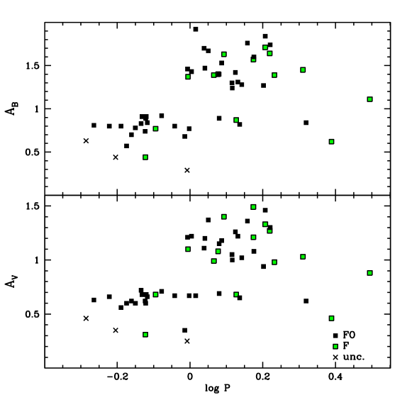
Figure 6: The same as in Fig. 3 but for Cepheids. Both amplitude distributions, $A_{V}$ (bottom panel) and $A_{B}$ (top panel), clearly show that our Cepheid sample forms two clusters of stars distinguished by small amplitudes for log P  $\sim$$<$  0, and larger amplitudes for log P  $\sim$$>$  0. Stars are color-coded according to their classification as derived in Section 5. Filled green and black squares correspond to FU and FO pulsators respectively. Crosses indicate those stars with uncertain mode classification (see the text for details).

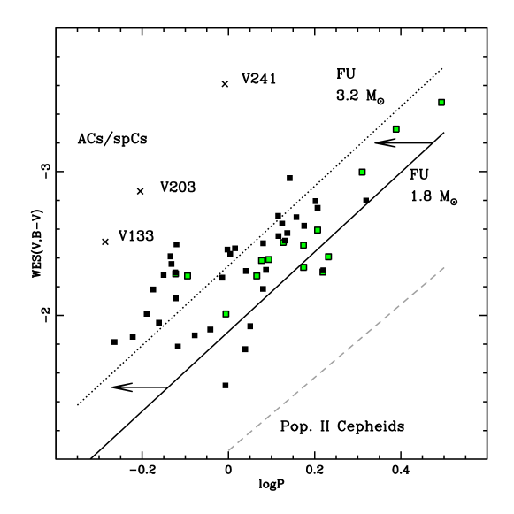
Figure 7: The Wesenheit distribution for RRLs and Cepheids. The same color code as in Fig. 6 has been used. The theoretical Wesenheit relations for stars with masses of 1.8 and 3.2 M_⊙ pulsating in the fundamental mode (solid and dotted lines, respectively) are shown, as predicted by Fiorentino et al. (2006). Arrows indicate the offset of the 1.8 M_⊙ first-overtone (FO) locus from the FU locus. For comparison, the location of Population II Cepheids is also indicated by a dashed line (Di Criscienzo et al. 2007).

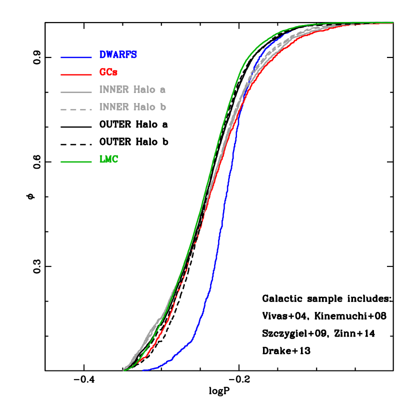
Figure 12: Cumulative period distributions for RRLs used to compute the likelihood that different samples are drawn from the same parent population. The data collected in this study represent: inner halo a (gray solid ine), inner halo b (gray dashed line), outer halo a (black solid line), outer halo b (black dashed line), classical dSph plus ultra-faint dwarf galaxies (blue solid line), GCs (red solid line) and LMC (green solid line).

Recently, extensive variability searches to characterize the RRL populations in UFDs have been carried out (Siegel 2006; Dall’Ora et al. 2006; Kuehn et al. 2008; Greco et al. 2008; Moretti et al. 2009; Musella et al. 2009; Dall’Ora et al. 2012; Musella et al. 2012; Clementini et al. 2012; Garofalo et al. 2013; Boettcher et al. 2013). Given the very small sample of RRL stars observed in most of the cases, it is very difficult even to provide a clear Oosterhoff classification for most UFDs. A few exceptions do exist: Bootes (11 RRLs, see Dall’Ora et al. 2006) is the sole example of an apparently well-established OoII type, whereas Ursa Major I (7 RRLs, see Garofalo et al. 2013) is classified as Oo-intermediate, resembling the classical dSph galaxies. Indeed, at the present date we might regard the distinction between UFDs and dSphs as largely a matter of semantics: according to the available evidence, the two terms may merely refer to the lower- and higher-mass members of a single family of objects (see, e.g., McConnachie 2012, especially Figs. 6, 7, and 12).

This paper is part of the effort of one of us (PBS) to establish and maintain a database of homogeneous photometry for resolved star clusters and galaxies. This effort seeks the greatest completeness and longest time span possible by exploiting public-domain data currently available from astronomical archives. In this paper we analyse in detail the properties of variable stars that we have identified in the Leo I dwarf spheroidal galaxy. Part of these data have already been presented in Fiorentino et al. (2012), where we focused our attention on understanding the intermediate-age central-helium-burning stellar population (Anomalous and/or short-period Cepheids, hereinafter AC/spCs). Here we present the full infrastructure underlying that discussion: identifications and equatorial positions for the complete set of variable star candidates together with their periods and light curve parameters. In §4 we describe in detail the RRLs of Leo I. In §5 we perform a slightly more detailed analysis of the AC/spC populations through mass determinations. Next, in §6 and §7 we discuss the variable stars in Leo I within the larger context of Milky Way formation and evolution discussed above. In particular we will compare the period distributions and period-amplitude relations of the RRLs in (a) our data for Leo I and literature data for other classical dSph galaxies with literature data for (b) the Galactic halo field, (c) the Galactic halo GCs, and (d) the new Galactic halo UFDs. A final summary discussion closes the main body of the paper. An Appendix addresses the reidentification of previously published variable candidates in Leo I.

2 Observations

The observational material for this study consists of 1,884 individual CCD images obtained on 48 nights during 32 observing runs. These data are contained within a much larger data collection ($\sim\,$400,000 images, $\sim\,$500 observing runs) compiled and maintained by the first author. Summary details of all 32 observing runs used here are given in Table 1. In fact, the observing runs designated “23 wfi4” and “24 wfi” were the same run, as were those designated “27 suba” and “28 suba2.” However, in each case different subsets of the images had been provided to us through different channels. To avoid any possible, unknown differences in the ways the images had been treated before we obtained them, we chose to keep them separate. Considering all the Leo I images together, the median seeing for our observations was 1^′′.0 arcseconds; the 25th and 75th percentiles were 0^′′.8 and 1^′′.3 arcseconds; the 10th and 90th percentiles were 0^′′.7 and 1^′′.6 arcseconds.

The photometric reductions were all carried out using standard DAOPHOT and ALLFRAME procedures (Stetson 1987, 1994) to perform profile-fitting photometry, which was then referred to a system of synthetic-aperture photometry by the method of growth-curve analysis (Stetson 1990). There were insufficient $U$-band observations from photometric occasions to establish a reliable $U$ magnitude system in Leo I, and we have made no attempt to calibrate those data photometrically. The few $U$-band images that we do have, however, were included in the ALLFRAME reductions to exploit whatever information they can provide on the completeness of the star list and the precision of the astrometric positions.

Calibration of these instrumental data to the photometric system of Landolt (1992) (see also Landolt 1973, 1983) was carried out as described by Stetson (2000, 2005). If we define a “dataset” as the accumulated observations from one CCD chip on one night with photometric observing conditions, or one chip on one or more nights from the same observing run with non-photometric conditions, the data for Leo I were contained within 95 different datasets, each of which was individually calibrated to the Landolt system. Of these 95 datasets, 63 were obtained and calibrated as “photometric,” meaning that photometric zero points, color transformations, and extinction corrections were derived from all standard fields observed during the course of each night, and applied to the Leo I observations. The other 32 datasets were reduced as “non-photometric”; in this case, color transformations were derived from all the standard fields observed, but the photometric zero point of each individual CCD image was derived from local Leo I photometric standards contained within the image itself; these local standards were established by us from the images obtained during photometric conditions. Considering the 95 datasets employed here, the median values for the root-mean-square residuals of the observed results for the standard stars relative to their established standard values were 0.029 mag in $B$ (minimum 0.007, maximum 0.079), 0.026 in $V$ (0.011, 0.076), 0.024 in $R$ (0.007, 0.059), and 0.024 in $I$ (0.011, 0.090). The (minimum, median, maximum) numbers of standard-star observations contained in each dataset were (88, 1644, 15084) in $B$, (79, 2059, 25664) in $V$, (85, 1440, 8742) in $R$, and (26, 1526, 14790) in $I$.

The different cameras employed projected to different areas on the sky, and of course the telescope pointings differed among the various exposures. Furthermore, the Wide-Field Camera on the Isaac Newton Telescope, the Wide-Field Imager on the 2.2m MPG/ESO telescope on La Silla, Suprime-Cam on the Subaru Telescope, FORS on the VLT on Paranal, and LBC on the Large Binocular Telescope on Mount Graham consist of mosaics of non-overlapping CCD detectors. The last column of Table 1 gives the number of independent detectors in each camera when this number is greater than one. Therefore, although we have 1,884 images, clearly no individual star appears in all those images. In fact, no star appeared in more than 97 $B$-band images, 240 $V$ images, 51 $R$ images, or 41 $I$ images. The median number of observations for one of our stars is 22 in $B$, 72 in $V$, 24 in $R$, and 16 in $I$. Since most pointings were centered on or near the galaxy, member stars typically have more observations than field stars lying farther from the galaxy center.

Our complete photometric catalog for Leo I and a stacked image of the field are available at our web site

3 Variable star detection and characterization

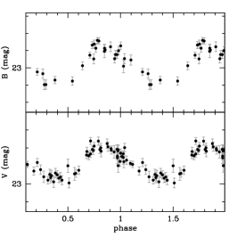
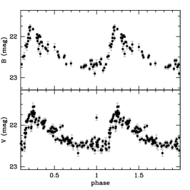
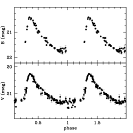
Figure 1: Examples of our light curves to illustrate the quality obtained in the $B$ and $V$ bands. We have selected one RRc (V60, left panel), one RRab (V92, possibly a Blazhko or double-mode pulsator candidate, middle) and one AC (V120, right). This last star has the uncommon 1 d period, but with our twenty-year baseline aliasing is minimal.

We have used an updated version of the Welch & Stetson (1993) method to identify candidate variable stars on the basis of our multi-band photometry of Leo I. We have identified 251 variable star candidates in a luminosity range that goes from the Horizontal Branch (HB) to the tip of the red giant branch (TRGB). A first guess at the variability period of each star was found using a simple string–length algorithm (Stetson et al. 1998b), then a robust least-squares fit of a Fourier series to the data refined the periods and computed the flux-weighted mean magnitudes and amplitudes of the light curves (Stetson et al. 1998b; Fiorentino et al. 2010, and references therein). The resulting pulsation properties are listed in Tables 2, 3 and  4. This list includes 164 stars that we have classified as RRLs, 55 AC/spCs and 19 LPVs. There are also thirteen more variable candidates whose physical nature is unclear (Table 5). Some of their light curves are shown in Fig. 1, and all are available in the on–line version of the paper and at our web site.

On the basis of the photometric quality of the data and the completeness of the phase coverage we have divided the pulsating variable candidates into three quality classes, namely: high confidence or “good” (A), uncertain or “fair” (B) and very uncertain or “poor” (C). These grades are given in Tables 2 (RR Lyraes) and 3 (AC/spCs). Among the 164 stars classified as RRL, we have assigned 95 A’s, 47 B’s, and 22 C’s; among the 55 AC/spCs there are 53 A’s, no B’s, and 2 C’s. In the case of a star classified as “A” we are reasonably confident that our pulsation properties are “essentially” correct; i.e., we believe that the period is correct to better than $\sim\,$1%, and the amplitudes are correct to 0.1–0.2 mag. For stars classed “B” there is a small ($<\,$25%?) chance that one or more parameters are wrong by more than this, and for stars classed “C” we feel that the chance of an error larger than this might be as high as 50%. These quantitative likelihoods are purely the educated guesses of a fairly experienced observer. We invite interested readers to examine the light curves and/or download our original data from our web site and judge the reliability of our inferences for themselves. We anticipate that future reinvestigations based upon new data will be able to retroactively establish how meaningful our subjective quality classes truly are.

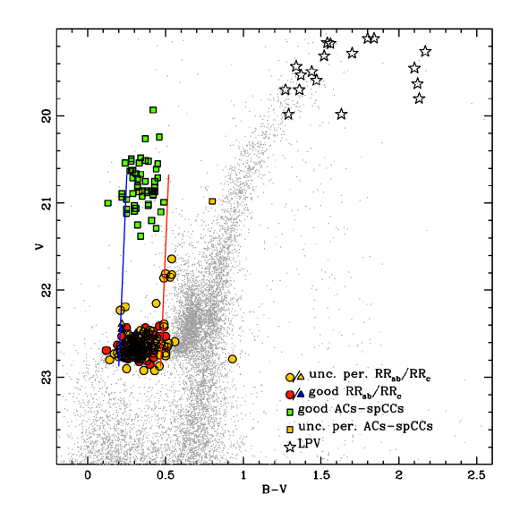
Figure 2: CMD and topology of the instability strip for the variable stars of Leo I. Red circles and blue triangles represent RR Lyrae stars pulsating in the fundamental and first-overtone mode, respectively. Squares and stars represent Cepheids and LPV variables. Variable candidates with uncertain periods are indicated by yellow symbols.

In Fig. 2 we show the locations in the CMD of these variable star candidates and the theoretical instability strip (IS) derived from radial nonlinear pulsating models for AC/spCs (Marconi et al. 2004; Fiorentino et al. 2006) and RRLs (Di Criscienzo et al. 2004). We have not included here the thirteen variables that we have not been able to characterize (see Table 5). The agreement between the locations of “good” RRLs (blue and red dots) and AC/spCs (green squares) and the theoretical boundaries of the IS is excellent with very few exceptions. We also show the possible LPV candidates (stars); they are all located near the TRGB and the upper asymptotic giant branch (see Table 4). Unfortunately, the sampling of our light curves for the LPVs is neither dense nor well distributed over the necessary range of time intervals, and we could not reach any definitive evaluation of their periods. Detailed periods, being related to the LPV’s masses and ages, could have provided constraints on the star formation history of the galaxy (see Feast & Whitelock 2013, and references therein). The so-called “periods” that we give in Table 4 are formal maximum-likelihood values returned by our software, but they should be regarded as purely notional. We provide them only to give some sense of the timescales upon which the variations appear to be occurring. We commend these stars to the attention of individuals having extensive access to telescopes of moderate aperture.

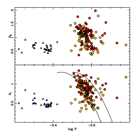
Figure 3: Bailey diagram for RRL stars in the $B$ (top panel) and $V$ bands (bottom panel). Symbols are as in Fig. 2. We have also shown, as solid curves, the empirical relations for Oosterhoff types I (left) and II (right) as derived by Cacciari et al. (2005).

Our sample of 164 RRL candidates contains 95 good stars (see Table 2) including 24 that apparently either show the Blazhko effect or pulsate in multiple modes. Among the good RRLs we recognize 14 first overtone (FO) and 81 fundamental-mode (FU) pulsators on the basis of their period/amplitude distribution in the Bailey diagram (see Fig. 3). The remaining 69 RRL candidates with fair and poor light-curve fits are provisionally divided into 14 FO (12 “B” and 2 “C”) and 55 FU (35 “B” and 20 “C”) pulsators. The pulsation properties of the RRL sample will be discussed in more detail in the next section.

The sample of AC/spCs is quite abundant, populating the whole theoretical IS, and consists of 55 objects (see Table 3), including two with uncertain or very uncertain periods (V212 and V241). Our sample also includes one possible Blazhko or multiple-mode Anomalous Cepheid, V129. The evolutionary classification of these stars has been discussed in a companion paper (Fiorentino et al. 2012) and will not be repeated here, but in Section 5 we will place some constraints on their masses and mode classification.

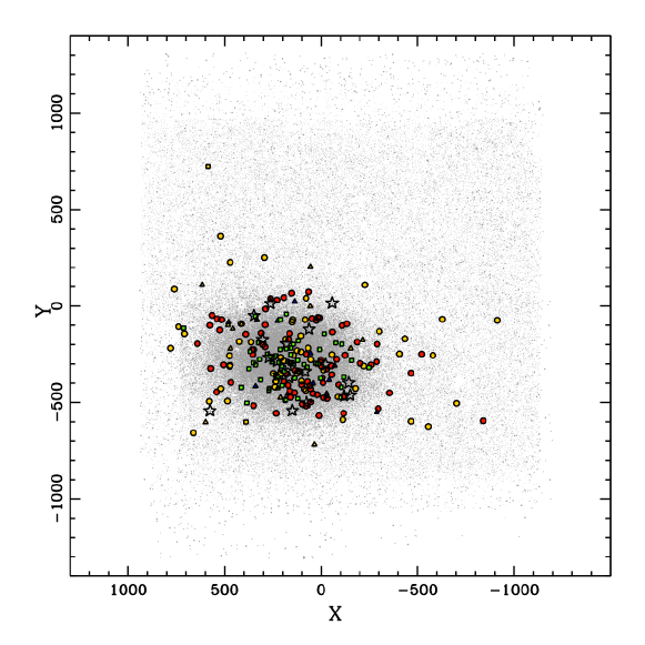
Figure 4: Distribution of our variable candidates in the field of view of our photometric study. The symbols for variable stars are color-coded as in Fig. 2. Gray dots represent non-variable stars and are expanded according to their brightness in the $V$ band. Units are arcseconds relative to an arbitrary origin (stated in text); X increases east (to the left) and Y increases north (up). An ellipse represents an isopleth of the stellar distribution with a semimajor axis of 12^′ as derived by Mateo et al. (2008).

The spatial locations of all our variables are shown in Fig. 4. The $(x,y)$ coordinates in this diagram are referred to an origin $(0,0)$ that we have arbitrarily placed at 10^h08^m16^s.21 +12^∘23^′05^′′.0 (close to the center of an early subset of our images). The $y$-axis is the great circle $x=0$ and is equal to the great circle $\alpha$ = 10^h08^m16^s.21, and the $x$-axis is tangent to $\delta$ = +12^∘23^′05^′′.0 at the origin. The photocenter of Leo I has been estimated to lie at $(\alpha,\delta)=(152.1125,12.30833333)$ (= 10^h08^m27^s.00 +12^∘18^′30^′′.0) according to Mateo (1998); we ourselves estimate the center of Leo I to lie at 10^h08^m27^s.13 +12^∘18^′22^′′.2 [$(x,y)=(+160.0,-282.8)$], with an uncertainty of order 1^′′ in each coordinate. This estimate has been derived by determining the median $x$ and $y$ coordinates of probable member stars lying within a range of distances from the center, from 100^′′ to 850^′′; the consistency of these values provides our estimate of the uncertainty (see Stetson et al. 1998a, §3.4). Fig. 4 shows that the RRLs, as representative very old stars, have a larger spatial extent than the younger, more massive stars that we presume the AC/spCs and LPVs to be; the latter appear more centrally concentrated. This supports the idea that AC/spCs in Leo I are of the same nature as those in the Large Magellanic Cloud (LMC), where ACs seem to result from both the intermediate-age stellar population and old binary systems (Fiorentino & Monelli 2012). This is consistent with our provisional classification of these stars as a mix of both ACs and spCs (see Fiorentino et al. 2012, for details).

4 RR Lyrae stars

The Bailey diagrams are shown in Fig. 3 for the $B$ (top) and $V$ (bottom) photometric bands. As expected, the RRLs separate very cleanly into two different groups, the longer-period FU pulsators (log P  $\sim$$>$  –0.35, P  $\sim$$>$  0.45 d: RRab or, to some researchers, RR0) and the shorter-period FO pulsators (log P  $\sim$$<$  –0.35: RRc, or RR1). These diagrams are very often used to give an indication of the Oosterhoff class. For this reason, in the $V$-band (bottom) panel we have also plotted the curves (Cacciari et al. 2005) representative of the Oosterhoff dichotomy shown by RRab stars in Galactic GCs. We note that most of the RRab stars seem to follow the OoI line, reaching a maximum $A_{V}$ amplitude of about 1.2 mag. However, as discussed in (Fiorentino et al. 2012), based on the mean period of the RRab sample we have classified Leo I as Oo-intermediate, since $\left<\hbox{\rm Pab}\right>\,=$ 0.596$\pm$0.001 d ($\sigma$=0.05), based on only those stars with good light-curve fits. This result does not change when we include the RRab variables with fair or poor periods or when we add the RRc stars with fundamentalized periods (Coppola et al. 2013).

We have also calculated the ratio between the number of RRc and the total number of RRLs, which is considered another indicator of Oosterhoff class, ${N_{\rm c}}/{(N_{\rm c}+N_{\rm ab})}=28/164\approx 0.17$. This value of the ratio includes the variable candidates with fair and poor light-curve fits; a slightly lower value, $14/95\approx 0.15$, is obtained when it is based on only the good RRLs. We have a slight preference for the higher value, however, because the very classification “good,”, “fair,” and “poor” disproportionately assigns the lower quality classes to the c-type variables with their smaller amplitudes. Although those same smaller amplitudes probably mean that the c-type variables are more affected by incompleteness even if we ignore the quality classes, these very small values of the c-to-total ratio still suggest that it would be hard for us to have missed enough c-type variables to push Leo I out of the the OoI class. This conclusion is in line with what has been observed in other nearby dSph galaxies (see section 6 for details).

We take advantage of the good sampling of our light curves, in particular in the $B$ and $V$ bands, to estimate the mean amplitude ratios $\left<A_{V}/A_{B}\right>=0.825\pm 0.002\,$mag ($\sigma\,$= 0.20) and $\left<A_{R}/A_{V}\right>=0.763\pm 0.004\,$mag ($\sigma\,$= 0.24), based on 95 and 63 RRLs respectively (not all stars with “A”-quality data in $B$ and $V$ have good data in $R$). This $A_{V}/A_{B}$ value is in full agreement with the value discussed in Di Criscienzo et al. (2011) based on 130 RRLs taken from nine GGCs.

4.1 Distance to Leo I from RRLs

In this section we use the RRL pulsation properties to constrain the distance to Leo I. In particular, we use two independent methods: a linear formulation of the $M_{V}$ versus [Fe/H] relation (Bono et al. (2003); see also Cacciari & Clementini (2003)) and the First Overtone Blue Edge (FOBE) method (Caputo et al. 2000, and references therein).

For the $M_{V}$ versus [Fe/H] relation we consider only the 81 RRab-type variables with light curves of quality class “A” (“good”), and we compare their measured properties to the following theoretical formulations:

$$M_{V}(RR)=(0.18\pm 0.07)\hbox{\rm[Fe/H]}+(0.72\pm 0.07),\quad\hbox{\rm for [Fe/H]$\,\leq\,-1.6\,$dex}$$

and

$$M_{V}(RR)=(0.36\pm 0.03)\hbox{\rm[Fe/H]}+(1.04\pm 0.08),\quad\hbox{\rm for [Fe/H] $>$ --1.6 dex}$$

(Bono et al. 2003). In order to use these formulae we must assume a metal abundance for Leo I. Recent measurements of the galaxy’s metallicity based on a large ($\sim\,$850) sample of individual RGB stars studied with medium-resolution spectroscopy have provided a mean metallicity of [Fe/H] $\sim$ –1.43 ($\sigma=$ 0.33 dex; Kirby et al. 2011). However, it is worth mentioning that Leo I seems to have a broad metallicity distribution, with iron abundances ranging from $\sim\,$–2.15 to $\sim\,$–1. RRLs being among the oldest and presumably the metal-poorest stars in a stellar system, we decided to derive two different distance moduli corresponding to both the average Leo I metallicity and the metal poor extreme. We found $\left<V\right>=22.648\pm 0.001\,$mag ($\sigma=0.11$) for the RRL sample, and assuming E(B–V) = 0.02 mag, the two distance moduli turn out to be $\mu_{0}=22.06\pm 0.08$ and $22.25\pm 0.07\,$mag for [Fe/H]$\,=\,$–1.43 and –2.15, respectively. These values are in good agreement with the distance modulus derived by Bellazzini et al. (2004) using the TRGB method: $\mu_{0}=$22.02$\pm$0.13 mag, corresponding to a heliocentric distance D$\,=\,254^{+16}_{-19}\,$kpc.

Now we use the technique extensively discussed in Caputo et al. (2000), which is a graphical method based on the predicted period-luminosity (PL) relation for pulsators located along the FOBE. It seems quite robust for clusters with significant numbers of RRc variables and is thus applicable to Leo I. The distance modulus is derived by matching the observed distribution of RRc variables to the following theoretical relation:

$$M_{V}\hbox{\rm\footnotesize(FOBE)}=-0.685(\pm 0.027)-2.255\log P\hbox{\rm\footnotesize(FOBE)}-1.259\log(M/M_{\odot})+0.058\log Z.$$

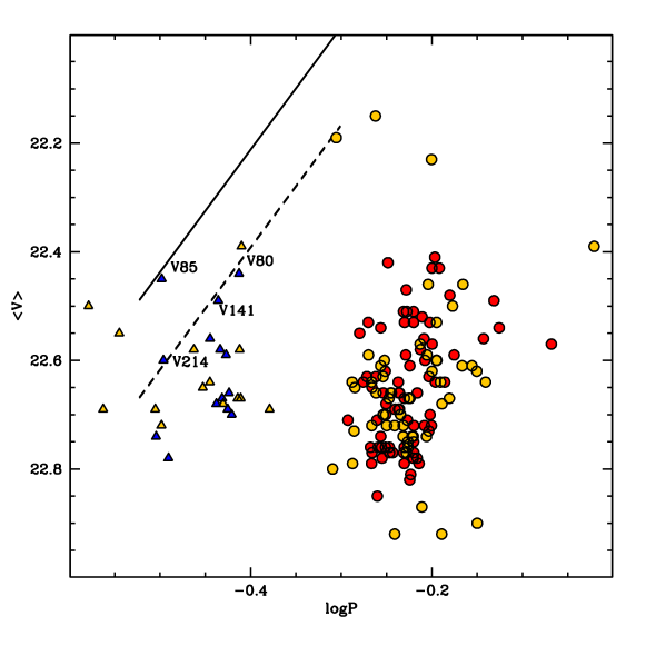
Figure 5: The period-luminosity distribution of RRLs in Leo I. The symbols are color-coded as in Fig. 2. The solid line corresponds to the FOBE position as constrained by V85, whereas the dashed one is drawn to match V80, V141, and V214.

Here, we assume the same two metallicity values for the RRLs in Leo I and adopt M = 0.7M_⊙ from the evolutionary HB models for RRc variables, with an uncertainty of the order of 4% (Bono et al. 2003). The comparison between the observed RRLs and the theoretical relation is shown in Fig. 5. Given the period-luminosity distribution of our RRc sample and the high uncertainty in the FOBE determination, we decided to use two possible FOBE evaluations, the first defined by the “good” RRc V85 and the other by V80, V141 and V214. Thus, the FOBE method returns a range of possible distance moduli, $\mu_{0}=$21.96 (V85) to 22.14 (V80,V141,V214) assuming [Fe/H]$=$–2.15 and E(B–V) = 0.02 mag; these decrease by 0.04 mag when using the metal-rich stellar content (–1.43 dex). It is worth noting that the distance evaluation based on the FOBE defined by V85 gives a distance determination that is also in very good agreement with that given by the TRGB method (Bellazzini et al. 2004).

5 Anomalous and short-period Cepheids

In a previous paper (Fiorentino et al. 2012), we discussed the evolutionary classification of the Cepheid sample we have detected in Leo I. On the basis of a comparison with a set of evolutionary tracks at different metallicities ([Fe/H] ranging from –1.8 to –1.0) we have concluded that we are dealing with an unprecedented mix of ACs and spCs. In this section, we discuss the pulsation properties of this unique sample of variable stars.

In Fig. 6 we show their distribution in the amplitude versus period diagrams in the $B$ (top) and $V$ bands (bottom). It seems clear that the sample can be divided into high- and low-amplitude subsamples separated at $A_{B}\sim 1.1$ and $A_{V}\sim 0.8$, with the low-amplitude stars dominating for periods less than one day and the high-amplitude stars dominating at longer periods. Similar behavior seen in other classes of pulsating variables, e.g., RRLs, usually identifies a mode separation between the first overtone (lower amplitudes, shorter periods) and fundamental (higher amplitudes, longer periods) modes of pulsation. However, for ACs the mode classification is far from trivial and cannot be easily linked to either the period-amplitude distribution or the morphology of the light curves, as discussed in Marconi et al. (2004).

We note that observational uncertainties probably do not contribute much to the scatter of points in the amplitude versus period diagrams. For the 53 out of 55 candidates to which we have assigned quality class “A,” we feel that the amplitude uncertainties are probably not worse than 0.1 mag and the period uncertainties are probably not larger than 1% ($\sigma(\log P)\sim 0.004$). These numbers are much smaller than the dispersion seen in Fig. 6. We conclude, therefore, that the spread is real and intrinsic to the stars themselves.

The distribution in the period-luminosity diagram might help in the mode classification. For this reason, in Fig. 7 we show the AC/spC distribution in the reddening-free ($V$,B–V) Wesenheit magnitude versus period plane. We have chosen this color combination because the available $B$ and $V$ observations best sample the light curves, resulting in the most accurate mean magnitudes. Uncertainties of a few$\,\times\,$0.01 mag in the adopted mean $B$ and $V$ magnitudes for the stars lead to uncertainties  $\sim$$<$  0.1 mag in the derived Wesenheit magnitudes. For comparison we have also shown the Wesenheit relations predicted by theoretical models for ACs assuming masses of 1.8 and 3.2 M_⊙ (Marconi et al. 2004; Fiorentino et al. 2006) and metallicities Z from 0.0001 to 0.0004, as well as those for Population II Cepheids (Di Criscienzo et al. 2004). We have assumed $\mu_{0}=$22.11 $\pm$ 0.15 with a reddening of E(B–V)=0.02 mag, values that were used by Fiorentino et al. (2012) to classify our sample of variable stars and that agree quite well with what is found using RRLs (see previous section). Our sample occupies the general region where ACs are expected without defining any tight sequence in this diagram. There are also no distinct subdistributions forming different sequences of AC/spCs such as are typically observed in other galaxies, where abundant samples of ACs (Fiorentino & Monelli 2012) and/or spCs (Bernard et al. 2013) show that both FU and FO pulsators are detected.

To investigate this behavior, we again use the approach discussed in Fiorentino & Monelli (2012), one that allows us to identify the mode classification within the sample of ACs in the LMC released by OGLE III (Soszyński et al. 2008). This method, detailed in Caputo et al. (2004), returns simultaneously the mode and the pulsation mass for each individual AC. It is based on the use of a theoretically predicted mass- and luminosity-dependent relation between period and $V$-band amplitude (MPLA) for FU mode pulsators, which is not followed by pulsators in higher modes. Coupling this relation with the mass-dependent period-luminosity-color (MPLC) relation that exists for both modes, we will assign the FU pulsation mode only when the two masses agree within 1$\sigma$. We use the following relations:

$$\log P_{F}+0.41M_{V}+0.77\log\hbox{\rm M}=0.01-0.188A_{V},$$

predicts the visual amplitude from the period, luminosity and mass for fundamental pulsators, and

$$M_{V}=-1.56-2.85\log P+3.51(\hbox{\it B--V\/})-1.88\log\hbox{\rm M}\quad\hbox{\rm(FU)},$$

$$M_{V}=-1.92-2.90\log P+3.43(\hbox{\it B--V\/})-1.82\log\hbox{\rm M}\quad\hbox{\rm(FO)}$$

predict the luminosity from the period, color and mass for FU and FO pulsators. These have been derived in (Marconi et al. 2004), and can be inverted to yield

$$\log[\hbox{\rm M/M${}_{\odot}$\footnotesize{(MPLA-FU)}}]=\bigl{(}0.01-0.188A_{V}-\log P-0.41M_{V}\bigr{)}/0.77$$

$$\log[\hbox{\rm M/M${}_{\odot}$\footnotesize{(MPLC-FU)}}]=-\bigl{(}M_{V}+1.56+2.85\log P-3.51(\hbox{\it B--V\/})\bigr{)}/1.88$$

$$\log[\hbox{\rm M/M${}_{\odot}$\footnotesize{(MPLC-FO)}}]=-\bigl{(}M_{V}+1.92+2.90\log P-3.43(\hbox{\it B--V\/})\bigr{)}/1.82.$$

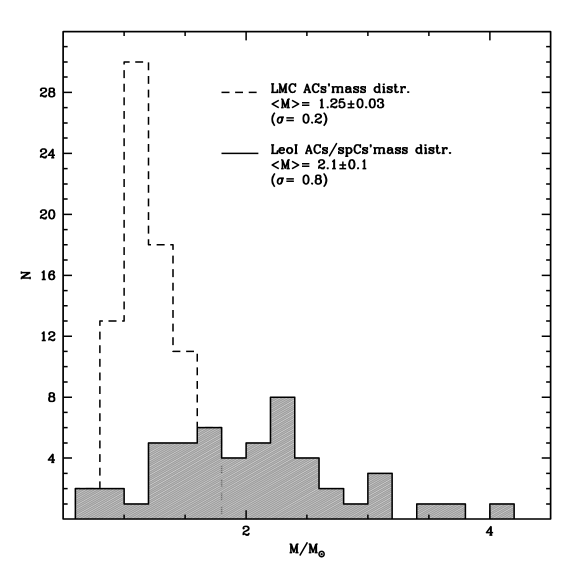
Figure 8: The mass distribution for Leo I  Anomalous and short-period Cepheids (black solid lines and gray fill) has been computed using the approach discussed in (Fiorentino & Monelli 2012). The mean mass and the standard deviation reported in the legend exclude six outliers with derived masses larger than 5 M_⊙. For comparison, the dashed lines show the mass distribution of ACs in the OGLE sample for the LMC. The mean mass of the LMC Cepheids has also been specified in the legend.

Our application of these equations produces the masses and the classifications given in Table 3 and summarized in Fig. 8. In this figure we show the mass distribution (gray histogram) predicted for our sample based on the pulsation relations. This is to be compared with the very peaked mass distribution shown by ACs observed in the LMC. This confirms our interpretation that a continuous spread in masses in Leo I causes the dispersion shown in the Wesenheit plane (see Fig. 7), whereas in the LMC you can perceive two distinct sequences in the same plane (Soszyński et al. 2008; Fiorentino & Monelli 2012).

Three AC/spCs in Leo I show unreasonably high masses, larger than 5 M_⊙ (indicated with crosses in Figs. 6 and  7); in Fig. 7 these stars are the ones deviating the most from the global distribution in the Wesenheit plane due to their very short periods compared to other stars with comparable luminosities and colors. In particular, the star with the highest indicated mass, V241, belongs to our “very uncertain” class (C) and shows a very red color (B–V$\,\geq\,$0.6), thus suggesting the possibility of problems in our magnitude, color and/or period determinations for this star. The other two stars, namely V133 and V203, show very small amplitudes (see Fig. 6) suggesting that they might be slightly blended. A visual examination of these stars in our stacked image for Leo I suggests that a blending explanation for their anomalous masses is plausible, but not definite.

6 Comparing Leo I with classical spheroidal and ultra-faint dwarf galaxies

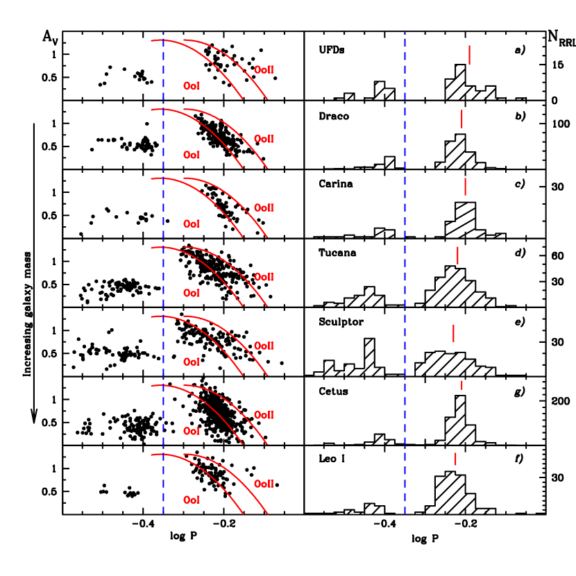
Figure 9: left – Period versus $V$-band amplitude diagram for RRLs observed in eleven UFDs (top panel) and six dSphs (remaining six panels) for which mostly complete samples of variable stars have recently been published. The galaxies have been ordered by increasing baryonic mass from top to bottom. The UFDs have been considered together to improve the statistical significance of the plot. right – Period-frequency distributions of the same RRLs; the mean period of the RRab variables is indicated by a vertical red line in each panel. The vertical blue dashed lines in this plot indicate $\log P=-0.35$, which we have taken as the nominal boundary between RRc (FO) and RRab (FU) variables.

In Figs. 9 and 10 we show the amplitude versus period diagrams (left) and the period histograms (right) for RRL and AC/spC stars in six dSphs ordered by increasing baryonic mass (McConnachie 2012), namely Draco (Kinemuchi et al. 2008), Carina (Coppola et al. 2013), Tucana (Bernard et al. 2009), Sculptor (Kaluzny et al. 1995), Cetus (Bernard et al. 2009; Monelli et al. 2012) and Leo I (this paper). In the top panel of each figure we have also shown all the RRLs and AC/spCs observed in the eleven UFDs surveyed for variability (Dall’Ora et al. 2006; Kuehn et al. 2008; Moretti et al. 2009; Musella et al. 2009; Dall’Ora et al. 2012; Musella et al. 2012; Clementini et al. 2012; Garofalo et al. 2013; Boettcher et al. 2013). For comparison, in Fig. 9 we also show the two curves that trace the Oosterhoff dichotomy observed in Galactic GCs as defined by Cacciari et al. (2005). Lying in general between the two Oosterhoff curves, the ab-type RRL distributions for the classical dwarfs in the Bailey diagram are very similar to each other. The only (slight) exceptions are Cetus and Carina, which show a different slope in the period versus amplitude plane as discussed in Bernard et al. (2009) and Monelli et al. (2012). For most dSphs, the period distributions of RRab stars (right panels of Fig. 9) are quite peaked around their mean value with two exceptions, viz. Sculptor and Tucana. In Table 6 we have listed the mean properties of the RRLs according to the catalogs we have adopted; the mean RRab and RRc periods are the same within 1$\sigma$. In the last column we have also listed the total masses and mean metallicities of these galaxies according to the references used in McConnachie (2012). The mean periods of RRLs in UFD galaxies seem to generally follow the same behavior as in classical dwarfs, occupying the same general location in the Bailey diagram with a slightly higher mean period for the RRab stars, very similar to that of Carina (Dall’Ora et al. 2003; Coppola et al. 2013). This suggests that, at least in terms of their RRL properties, there is not a significant difference between classical and ultra-faint dwarf galaxies.

On the basis of their similar general properties, we decided to build up a single large sample of well studied RRLs in those dwarf galaxies where the variability surveys do not seem to suffer from strong completeness problems, thus very likely describing the RRL properties of these stellar systems rather well. This initial sample contains 1,726 objects (with 1,299 ab-type variables); we included Cetus and Carina because their inclusion does not bias the mean properties of the sample nor change our final conclusions.

As discussed in Fiorentino et al. (2012), different conclusions result from an inspection of Fig. 10, where it is clear that the AC/spCs have different period distributions and Bailey diagrams. In particular, we note that the period distribution seems to move toward longer periods when the baryonic total mass of the galaxy increases (see Table 6). This is easily understood when one considers that the high masses typical of ACs (Fiorentino et al. 2012, 1.2 $\sim$$<$ M/M${}_{\odot}\;\lower 2.58334pt\hbox{$\sim$}\kern-9.2pt\raise 1.72218pt\hbox{$<$}\;$ 2.1) may result from either or both the interactions of old binary stellar systems and single-star evolution in purely intermediate-age populations. Thus, their specific frequency could depend on the total mass of the host galaxy and on the relative importance of star formation events at intermediate ages ( $\sim$$<$  5 Gyr), as extensively discussed by Fiorentino & Monelli (2012).

7 Comparing dwarf galaxies with globular clusters and the halo field

Usually, the average properties of RRLs in individual dSphs and UFDs—such as the mean periods of both RRab and RRc stars—are compared to those observed in GCs as representative of the Galactic halo (Catelan 2009; Clementini 2010, and references therein). However, given their different total stellar masses, GCs typically host RRL populations of order a factor 10 smaller than those observed in dwarf galaxies, making a proper statistical comparison frequently difficult. Moreover, in the last ten years or so, GCs have been demonstrated to be quite complex stellar systems despite what we previously believed in terms of their chemical enrichment histories (Gratton et al. 2004; Piotto et al. 2005; Milone et al. 2012; Monelli et al. 2013), and they may not fairly represent the properties of halo field stars. Even though the net effect of their complex histories on their global average chemical abundances (and therefore on the pulsation properties of their RRLs) may be negligible, this has not yet been demonstrated. Finally, although it seems trivial that the statistical meaning of averaged properties is, by definition, more significant when a large sample of objects is considered, we must remember that small number statistics become quite relevant in those galaxies with very few confirmed member RRLs, as is the case for most UFDs (Moretti et al. 2009; Musella et al. 2009; Dall’Ora et al. 2012; Clementini et al. 2012; Boettcher et al. 2013) where even the term “average” approaches meaninglessness.

The justification for our assembling a large sample of RRLs in classical and ultra-faint dSphs is driven in large part by the opportunity to compare directly, for the first time, their period and amplitude distributions with those of a huge RRL sample representing the Galactic halo. RRLs are ancient stars, older than 10 Gyr. Their younger selves were born during the early millennia of the Universe, and their testimony can provide important information about chemical evolution during the early stages of the assembly of the Galactic halo. Moreover, they are their own robust distance indicators that might also reveal details of the halo’s spatial structure (Layden 1994; Kinemuchi et al. 2006; Drake et al. 2013; Zinn et al. 2014).

With this goal in mind, we have collected several catalogs—mainly on the basis of the availability of robust periods and reliable $V$-band amplitudes—that, taken together, provide about 14,000 RRab stars spanning distances from $\sim\,$5 to $\sim\,$80 kpc, namely the QUEST (Vivas et al. 2004; Zinn et al. 2014), NSVS (Woźniak et al. 2004), ASAS (Szczygieł et al. 2009) and CATALINA surveys (Drake et al. 2013). In cases where a star appeared in multiple surveys, we have retained only those data originating in the most recent and complete study available.

We have computed the three-dimensional Galactocentric position of each individual RRL, first converting (RA,Dec) to (l,b) coordinates and then assuming for the stars in the very inner part of the Halo (d${}_{G}\,\;\lower 2.58334pt\hbox{$\sim$}\kern-9.2pt\raise 1.72218pt\hbox{$<$}\;\,$7.5 kpc) a mean metallicity of [Fe/H]$\,=\,$–1.3 dex, while for the external part we used –1.6 dex, according to the metallicity gradient reported by Layden (1994). To account for the individual interstellar extinctions we have used the Schlegel et al. (1998) maps, following the prescription given in their website. Finally we have applied the same magnitude versus metallicity relation for the RRLs as we used in Section 4 for [Fe/H]$\,>\,$–1.6 dex (Bono et al. 2003), assuming a distance to the Galactic Center of 7.94 kpc (Eisenhauer et al. 2003; Groenewegen et al. 2008; Matsunaga et al. 2011).

In our final catalog, we have not included the samples from Miceli et al. (2008) and Sesar et al. (2013) because amplitudes on their filterless magnitude system must be transformed into $V$ (Landolt) amplitudes using a metallicity- and temperature-dependent scale factor that could affect the stars’ apparent distribution in the Bailey diagram. On the other hand, we do include the CATALINA sample, while acknowledging that it has a bias in amplitudes; we retain only RRLs with amplitudes $A_{V}$ larger than 0.4 mag. However, this is the largest, deepest, and most homogeneous catalog at our disposal, and its known bias turns out to have a negligible effect on the following discussion. Finally, we use only ab-type RRLs because they are less affected by both time-sampling and completeness problems. Although not 100% complete, this final huge catalog will allow us to make the most comprehensive analysis of the Galactic halo using field RRLs possible so far.

In order to draw the most complete global view of the globular clusters belonging to the Galactic halo, we have decided to exclude all the RRLs listed in the updated catalog of Clement et al. (2001) that are observed in GCs belonging to the Galactic bulge, i.e., those having both Galactocentric distance d${}_{G}\,\leq 5\,$kpc and distance from the Galactic plane Z$\,\leq\,$1.5 kpc. Two exceptions to this rule are M62 (NGC 6266) and M28 (NGC 6626) that—even if projected onto the bulge region (Harris 1996)—can not be considered representative of the bulge population (Casetti-Dinescu et al. 2013, and reference therein). We have also excluded NGC 2419 because it is located in a region of the halo not well covered by the field-star surveys considered here. Finally, we have included only GCs for which CCD photometry in $V$, including amplitudes, is available. The full sample consists of 1,617 RRLs (1,054 ab-type) residing in 35 GCs (see Table 7).

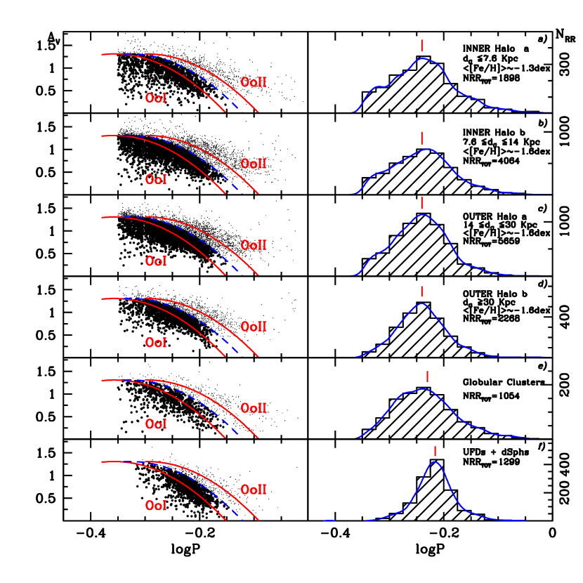
Figure 11: left – Period versus $V$-band amplitude diagram for RRab observed in the Galactic halo (panels a, b, c, d)), compared to GCs (panel e) and dSphs plus UFDs (panel f). The two Oosterhoff curves given in Cacciari et al. (2005) are also indicated together with a mean curve used to notionally separate the OoI from the OoII components (blue dashed line). right – Period distributions of RRab for the same samples plotted on the left. In each panel the smoothed histogram used to perform the statistical comparison discussed in the text are also plotted (blue solid curves).

In Fig. 11 we show the distributions of RRab stars in period-amplitude diagrams (left) and period histograms (right) for the full set of catalogs we have collected. The first four panels are devoted to the Galactic halo divided into four non-overlapping regions: 1) the inner halo a, consisting of stars with d${}_{G}\,\;\lower 2.58334pt\hbox{$\sim$}\kern-9.2pt\raise 1.72218pt\hbox{$<$}\;\,$7.5 kpc (panel a); 2) the inner halo b, stars with 7.5  $\sim$$<$  d${}_{G}\,\;\lower 2.58334pt\hbox{$\sim$}\kern-9.2pt\raise 1.72218pt\hbox{$<$}\;\,$14 kpc (panel b); 3) the outer halo a, stars with 14  $\sim$$<$  d${}_{G}\,\;\lower 2.58334pt\hbox{$\sim$}\kern-9.2pt\raise 1.72218pt\hbox{$<$}\;\,$30 kpc (panel c); 4) the outer halo b, stars with d${}_{G}\,\;\lower 2.58334pt\hbox{$\sim$}\kern-9.5pt\raise 1.72218pt\hbox{$>$}\;$30 kpc (panel d). The boundary between inner and outer halo (d${}_{G}\,\sim\,$14 kpc) has been chosen according to Kinman et al. (2012), whereas the other reference distances are arbitrary. In the last two panels, we have plotted the full distributions obtained for GCs (panel e) and UFDs+dSphs (panel f). As in Fig. 9, we have overplotted the Oosterhoff curves given by Cacciari et al. (2005). The average of their two curves (blue dashed curve in Fig. 11) allows us to roughly separate the two populations of OoI (large dots) and OoII (small dots) RRLs. We have computed the ratio between OoI and the total number of RRLs, as given in the last column of Table 7. These numbers are very similar to each other and they are compatible with a global OoI classification, in agreement with recent and independent results from the ROTSE (Miceli et al. 2008) and LINEAR (Sesar et al. 2013) surveys.

We have also used these data to compute the mean periods of the RRLs with log P$\,\geq\,$–0.35 (see Table 7), and find that $\left<\hbox{\rm Pab}\right>$ is the same within the standard deviations of the distributions. Again, the mean properties of the different RRab samples seem virtually indistinguishable from this statistical point of view.

To compare these distributions in more rigorous detail, we have performed two more sophisticated statistical analyses. The first is a chi-squared test on the histograms smoothed with a Gaussian filter (see blue solid curves in Fig. 11), and the second is a Kolmogorov-Smirnov test applied to the cumulative period distributions (see Fig. 12). For the purposes of these last two tests, only, we take advantage of the large sample of RRLs in the Large Magellanic Cloud that has been provided by the OGLE project (17,693 stars; Soszyński et al. 2009). Although the RRLs in the LMC have been surveyed in the $I$ band by OGLE, we decided to attempt to match the amplitude bias of the CATALINA sample by using only those stars with A${}_{I}\geq$ 0.26 mag. This corresponds to a scale factor $A_{V}/A_{I}=1.58$ as found by Di Criscienzo et al. (2011). These two statistical tests returned very similar results, which are listed in Table 8 and can be summarized as follows:

• Inner halo a and b have a likelihood of 30% of being drawn from the same parent populations. This likelihood increases dramatically to 90% when only the CATALINA survey is considered. As shown in Fig. 11, these two regions show broad period distributions including the longest-period RRLs.

• Outer halo a and b do not share a common period distribution, with each other or with the inner halo. Each component of the outer halo seems to have a more peaked distribution than that of the inner halo. In particular, outer halo b seems to show a relative deficiency of RRab stars with high amplitudes and short periods (hereinafter, “HASP”). This can not be attributed to a completeness effect because large amplitudes are the easiest ones to detect.

• The GC period distribution mildly resembles that of the RRLs in the inner halo (within $\sim\,$14 kpc, a$+$b). This is reasonable when we consider that 23 out of the 35 GCs considered here belong to this region. We note that this result must be viewed as preliminary because: 1) the GC period distribution strongly depends on the choice of GCs included in the full catalog; 2) GCs have their own space motions that may eventually tell us more about the halo region to which they belong, rather than where they happen to be currently located.

• The UFD$+$dSph distribution is quite different from the others. It is very peaked around the mean period (see Table 7). In particular, this distribution is quite lacking in HASP RRab stars compared to the others: none of the RRLs in dwarfs with high amplitude ($A_{V}\geq 1.0$) reaches periods P$\,\;\lower 2.58334pt\hbox{$\sim$}\kern-9.2pt\raise 1.72218pt\hbox{$<$}\;\,0.48\,$d (log P  $\sim$$<$  –0.32). Fundamental-mode RR Lyraes with large amplitudes and periods less than 0.48 d are quite common both in globular clusters and in the halo field. Even the relative deficiency of HASP RRab stars in outer halo b already noted above is not as complete as in the UFD$+$dSph sample. It is true that at the other extreme, UFDs are seen to help in filling out the long-period tail (cf. Fig. 9a) but—within the limited statistics available—they do not appear to contribute to the short-period tail.

• We find a very low formal likelihood that the LMC sample matches any of the others (see Table 8), as is also true for classical dSphs and UFDs. We note here, though, that this result may be affected by the very high temporal and photometric completeness of the OGLE sample for the LMC. In other words, when huge samples are available (as they are here for the LMC and the Milky Way halo), any minor difference in selection biases achieves very high statistical significance and can be mistaken for a real physical difference between the samples. A fair comparison with the LMC sample needs much more complete RRL surveys of the Galactic halo. The same consideration is relevant to the recent result discussed by Zinn et al. (2014) where, on the basis of the OGLE (Soszyński et al. 2009) and their own QUEST RRL samples, the authors declined to exclude the possibility that the smooth Galactic halo may have formed from a combination of LMC- and Sagittarius-like galaxies. We believe—but are unable to prove—that because our comparisons between the halo, the GCs, and UFD+dSphs are based on samples closer in size, and probably with selection effects more nearly similar to each other than to the OGLE LMC sample, our conclusions regarding the statistical significance of their differences are probably more reliable than similar conclusions relating to the LMC.

8 Discussion: Building up the Galactic Halo with dwarf galaxies

Perhaps it is worthwhile to remind the reader that the dwarf galaxies in the Milky Way halo contain stellar populations with some range of ages and metallicities. The classical globular clusters as a class exhibit a broad range of metallicities ($-2.5<\hbox{\rm[Fe/H]}<0.0$, roughly speaking) and a rather limited range of age. The Milky Way field halo also clearly has a broad range of metal abundances, but we have less information as to its range of age. The range of metal abundance in the dwarf galaxies is somewhat narrower than among the GCs, [Fe/H]  $\sim$$<$  –1 or so, but some—including Leo I, Carina, and Fornax, for example—have very broad ranges of age, much greater than the range found among the GCs.

However, it must also be remembered that the range of age and metal abundance that is conducive to the formation of RR Lyraes is more restricted: the most metal-rich globular clusters contain no RR Lyraes, and the most metal-poor contain few, while moderately metal-poor clusters contain the most. Populations younger than $\sim 10\,$Gyr probably cannot produce RR Lyraes by the normal evolution of single stars. The range of metallicities where the globular clusters and the field halo are proficient at producing RR Lyraes, $-1.0\;\lower 2.58334pt\hbox{$\sim$}\kern-9.2pt\raise 1.72218pt\hbox{$<$}\;\hbox{\rm[Fe/H]}\;\lower 2.58334pt\hbox{$\sim$}\kern-9.2pt\raise 1.72218pt\hbox{$<$}\;-2.0$, is very well represented in the dwarf galaxies, and, as we have just mentioned, stars in the dwarf galaxies have—if anything—a broader range of age than those in the globular clusters and the field halo. That being the case, it is remarkable that there exists a class of RR Lyrae star that is present in the globular clusters and the field halo and absent in the dwarf galaxies. One would think that if there were some odd corner of age-metallicity space that is capable of making a particular class of RR Lyrae stars, but is not populated among the globular clusters, that niche would be more likely to be occupied in the dwarf galaxies: if anything, the dwarf galaxies should have more varieties of RR Lyrae stars than the globular clusters, not fewer.

One possible exception to this rule might be if the HASP RR Lyrae stars were uniquely the progeny of stellar collisions or merged gravitational-capture binaries; such stars could then be present in the globular clusters and not in the much sparser dwarf galaxies. But if this is the case, then why are these “special” RR Lyraes also found in the field halo, in roughly the same relative numbers as in the globular clusters? To be consistent, this explanation would suggest that a major fraction of the field halo stars came from globular clusters that were disrupted recently, i.e., only after the globular clusters had had enough time to produce the usual numbers of stellar collisions and gravitational-capture binaries. But even this seems highly unlikely, since halo field red giants do not show the light-element (C, N, O, Na, Mg, Al, etc.) correlations and anti-correlations found among the globular cluster giants.

In conclusion, and for the sake of argument, let us assume that in the early days of the Galactic halo, star formation occurred in one fundamentally indistinguishable family of structures, ranging in mass, that all underwent a common process of internal chemical evolution. During this time the young main sequence stars that grew into today’s RR Lyraes were born. During subsequent dynamical evolution most of these structures dissolved or were disrupted, releasing the globular clusters and field stars of today’s Galactic halo. At the same time a few of those structures—by random chance—survived, continued evolving internally, and became the classical dSph and UFD galaxies that we see today.

It seems that on the basis of the available RRL samples we can say that this scenario is not supported. Neither the inner (d${}_{G}\,\;\lower 2.58334pt\hbox{$\sim$}\kern-9.2pt\raise 1.72218pt\hbox{$<$}\;\,$14 kpc) nor the outer (d${}_{G}\,\;\lower 2.58334pt\hbox{$\sim$}\kern-9.5pt\raise 1.72218pt\hbox{$>$}\;\,$14 kpc) regions of the Galactic halo, nor any linear combination of the two, can be formed simply from the progenitors of today’s classical dSph or UFD galaxies. If present in sufficient numbers, structures like those that became today’s UFDs may have contributed to the long-period tail of the Galactic halo RRL period distribution, but—barring a major statistical fluke—neither they nor the dSph progenitors appear to have been capable of producing the kind of main sequence stars that became the HASP RRab variables now found in significant numbers throughout the Galactic halo and in the globular clusters.

Unless it can be shown that a protracted residence within the environment of a dSph or UFD galaxy can somehow alter the internal structure and evolution of an isolated star between the main sequence and RR Lyrae phases of its life, it seems that the simple model—where the dSphs and UFDs are surviving examples of representative proto-halo fragments—is disfavored. Instead it seems that already at the time when the future RR Lyrae stars were being born, the milieux that were halo-to-be or UFD/dSph-to-be were already different in some way. In other words, the progenitors of the Milky Way halo and of the surviving dwarf galaxies appear to have been different, non-representative subsamples of the proto-Galactic material, perhaps coming preferentially from distinct ranges of mass or kinematic properties, possessing different typical ratios of baryonic to dark matter, or being distinguished in some other relevant characteristic. Furthermore, the RRLs within the Galactic halo itself seem to have different period distributions when our consideration moves from the inner to the outer regions. This argues that the halo is itself formed from at least two different classes of progenitor or distinct, non-representative subsamples of a continuum of progenitors (see also Chiappini et al. 2001), as confirmed by kinematical surveys (Carollo et al. 2007; Kinman et al. 2012).

As was pointed out by an astute referee, there is now good evidence that all the known dSph and UFD galaxies—except Hercules—and the “young halo” globular clusters are distributed on a thin, rotationally supported planar structure containing the Galactic poles (the VPOS: Vast POlar Structure; Pawlowski et al. 2012; Pawlowski & Kroupa 2013). It seems far more likely that the VPOS and the distinct star systems located within it result from the disruption of a single infalling object, rather than from the isotropic accretion of a large number of smaller structures. This interpretation is inconsistent with the predictions of classical $\Lambda$CDM models for the formation of the halo in its entirety, but is consistent with our inference that the progenitor(s) of the UDF and dSph galaxies were different from the progenitor(s) of the Milky Way field halo stars and normal globular clusters.

As a final remark, since GCs represent only a small fraction of the Galactic halo, and because we now recognize that their histories were probably more complicated than we used to think—and are still not really understood—we would like to suggest that their continued use as representative tracers of the Galactic halo is not necessarily preferable to other comparisons that are now becoming possible.

We plan to extend this work to other dwarf spheroidal and irregular galaxies that are being studied within the homogeneous photometry project; we expect this will provide an opportunity to further test our conclusions.

9 APPENDIX: Previously identified stars

Leo I was previously surveyed for bright variable stars by Hodge & Wright (1978), who identified candidate Anomalous Cepheids and RR Lyraes, and by Menzies et al. (2002), who identified candidate long-period variables.

Hodge & Wright did not publish coordinates for their stars, but they did provide a finding chart. We extracted a JPEG version of their finding chart from the on-line electronic edition of their article and converted it to FITS format. Using a slightly modernized version of the Stetson (1979) software for astrometry and photometry from digitized photographic plates, we measured the positions of stars within the Hodge & Wright finding chart. We then used quadratic equations to transform those positions to the coordinate system of our Leo I catalog. We were able to match 355 stars within a tolerance of 4^′′ (the r.m.s. residuals were 0^′′.45 in right ascension and 0^′′.37 in declination). We were then able to geometrically transform their finding chart and overlay it on our stacked digital image of Leo I. Overall, we feel we are able to recover positions from the Hodge & Wright finding chart with a precision better than 0^′′.5. We considered stars within several arcseconds of each of the positions indicated in the published chart, basing our identification on (in order of decreasing importance) (1) evidence of variability in our data, (2) relative proximity to the indicated position, and (3) similarity of the mean $B$-band magnitude. We summarize our resulting cross-identifications in Tables 2 (RR Lyrae stars), 3 (AC/spC stars) and 9 (stars whose variability we are unable to confirm).

Notes on individual stars:

• The tick marks for HW1 in their chart enclose nothing but blank sky in our image. However, there are two of our variable candidates within 5^′′ of this position: V66 is a candidate long-period variable with $\left<B\right>\approx 22.1$ lying 4^′′.2 from the predicted position, and V59 is an AC/spC with P$\,=\,1.49328\,$d, $\left<B\right>\approx 20.7$ lying 4^′′.8 from the predicted position. Despite its greater offset, the latter star more closely resembles HW1 and we accept it as the match.

• HW2 has no detectable star in our image within the tick marks on the finding chart. There is a spot of fuzz most likely representing a galaxy about 1^′′ southwest of the indicated position, but this is probably too faint to have been detected in Hodge & Wright’s photographic material. One of our AC/spC candidates does lie almost 6^′′ ($>10\sigma$) from the indicated position. Since it has approximately suitable period and magnitude, we provisionally make this identification despite the large offset.

• HW20 has at least eleven stars lying closer to the indicated position than our adopted match, but the one we have chosen is clearly the most suitable on the basis of its mean $B$-band magnitude, and furthermore its Welch/Stetson variability index is not far below the detection threshold that we had imposed. This star may be variable, but we are not confident enough to claim definite confirmation.

Menzies et al. (2002) did not publish a finding chart for their five stars in Leo I. They did publish a table of equatorial coordinates for five luminous red stars in the galaxy field, but unfortunately we have not been able to find any relationship whatsoever between those coordinates and reality: we have marked their coordinates on our digital image of Leo I and we have also marked all the stars that are both luminous and red in our catalog, and we are not able to recognize any correspondence between the two patterns. For example, their stars A and B constitute a pair separated by 29^′′.7, slightly inclined with respect to the east-west direction. We have examined our list of luminous red stars for pairs separated by $\sim$30^′′, slightly inclined to the east-west direction, and do find a few. But when we accept any of those provisional matches none of the other three stars from Menzies et al. coincides with anything interesting.

Azzopardi et al. (1986) published a finding chart identifing several luminous, red stars in Leo I, and we give cross-identifications with our catalog in Table 10.

Table 1: Leo I Observations

Run ID	Dates	Telescope	Camera/Detector	$U$	$B$	$V$	$R$	$I$
1 nbs	1983 01 08-11	CTIO 4.0m	RCA	–	13	17	4	–
2 p200	1986 01 19-20	Palomar 5.1m	4-Shooter	–	–	17	11	–
3 f8	1986 02 19	CTIO 4.0m	RCA	–	12	–	–	–
4 km	1986 05 10-14	INT 2.5m	RCA	–	5	2	4	1
5 f10	1989 03 07	CTIO 4.0m	TI1	–	6	6	3	–
6 f9	1989 03 15	CTIO 0.9m	RCA5	–	4	4	4	–
7 f16	1992 03 06	CTIO 4.0m	Tek1K-2	–	5	5	–	–
8 demers	1992 03 26-27	CFHT 3.6m	Lick2	–	7	7	–	–
9 schommer	1992 05 31	CTIO 0.9m	Tek1K-1	–	–	2	–	–
10 f15b	1994 02 06	CTIO 0.9m	Tek1024	–	–	1	–	1
11 f15c	1994 03 13	CTIO 0.9m	Tek1024	–	–	1	–	1
12 bond	1994 12 03	KPNO 4.0m	t2kb	3	3	3	–	3
13 feb95	1995 02 04-05	Steward Bok 2.3m	12x8bok	–	–	72	–	–
14 mdm(a)	1995 02 27	Hiltner 2.4m	Charlotte Tek 10242	–	–	4	–	–
15 jka	1995 03 24	INT 2.5m	TEK3	–	–	1	–	–
16 apr95	1995 04 29-05 01	Steward Bok 2.3m	12x8bok	–	–	26	–	–
17 mdm(b)	1995 05 05	Hiltner 2.4m	Charlotte Tek 10242	–	–	4	–	–
18 bond2	1996 03 13	KPNO 4.0m	t2kb	1	1	1	–	1
19 int	1998 06 24	INT 2.5m	WFC EEV42	–	1	1	–	1	$\times\,$4
20 wfi3	1999 03 17	ESO 2.2m	WFI	–	–	13	–	13	$\times\,$8
21 emmi	1999 04 14-15	ESO NTT 3.6m	EMMI	–	6	6	–	1
22 fors9912	1999 12 02	ESO VLT 8.0m	FORS1	–	–	3	–	3
23 wfi4	2000 04 21-26	ESO/MP 2.2m	WFI	–	13	31	–	2	$\times\,$8
24 wfi	2000 04 22	ESO/MP 2.2m	WFI	–	4	10	6	1	$\times\,$8
25 tng	2001 01 24-26	TNG 3.6m	LRS Loral	–	30	49	–	–
26 bellaz	2001 03 19-22	TNG 3.6m	LRS Loral	–	–	8	–	8
27 suba	2001 03 20	Subaru 8.2m	SuprimeCam	–	–	–	7	–	$\times\,$8
28 suba2	2001 03 20-21	Subaru 8.2m	SuprimeCam	–	–	28	16	–	$\times\,$8
29 fors0204	2002 04 13	ESO VLT 8.0m	FORS2 MIT/LL mosaic	–	–	4	–	4	$\times\,$2
30 abi36	2002 11 13-15	KPNO 0.9m	s2kb	–	3	3	3	3
31 lbt(a)	2006 11 21-25	LBT 8.4m	LBC	43	20	–	–	–	$\times\,$4
32 lbt(b)	2006 12 16	LBT 8.4m	LBC	–	–	5	–	–	$\times\,$4

Note. — 1. Observer N. Suntzeff; 2. Observer R. Schommer?; 3. Observer N. Suntzeff or R. Schommer?; 4. Observer “KM”; 5. Observer N. Suntzeff or R. Schommer?; 6. Observer N. Suntzeff or R. Schommer?; 7. Observer N. Suntzeff or R. Schommer?; 8. Observer D. Crampton and J. Hutchings; 9. Observer R. Schommer; 10. Observer N. Suntzeff or R. Schommer?; 11. Observer N. Suntzeff or R. Schommer?; 12. Observer H. E. Bond; 13. Observer N. Suntzeff or R. Schommer?; 14. Observer unknown; 15. Observer “JKA”; 16. Observer N. Suntzeff or R. Schommer?; 17. Observer unknown; 18. Observer H. E. Bond; 19. Observer unknown; 20. Program ID unknown, observer unknown; 21. Program ID 63.H-0365(A), observer unknown; 22. Program ID 64.N-0421(A), observer unknown; 23. Program ID unknown, observer unknown; 24. Program ID 065.O-0530, PI Saviane, observer Momany; 25. Observer Bono; 26. Observer “bellaz”; 27. Proposal ID o00103, observers Arimoto, Ikuta, and Jablonka; 28. Proposal ID o00103, observers Arimoto, Ikuta, and Jablonka; 29. Program ID 69.D-0455(B), observer unknown; 30. Proposal ID “Saha”, observers Dolphin and Thim; 31. Observer unknown; 32. Observer unknown.

Table 2: RR Lyrae candidates: periods, photometric parameters and positions.

ID	Var	period	$\left<B\right>$	$\left<V\right>$	$\left<R\right>$	$\left<I\right>$	$A_{B}$	$A_{V}$	$A_{R}$	$A_{I}$	Q	RA	Dec
	type	d	mag	mag	mag	mag	mag	mag	mag	mag		hh mm ss	dd mm ss
V1*	RRab	0.515750	23.72	22.79	21.60	—	—	1.62	—	—	C	10 07 13.92	+12 21 50.8
V2*	RRab	0.627407	22.99	22.53	22.14	—	1.14	1.17	0.96	—	A	10 07 18.89	+12 13 10.2
V3*	RRab	0.554130	23.04	22.61	22.31	—	0.84	1.03	—	—	B	10 07 28.27	+12 14 40.4
V4*	RRab	0.638565	22.88	22.53	22.50	—	1.01	0.93	—	—	B	10 07 33.35	+12 21 56.1
V5*	RRab	0.593564	23.25	22.75	22.46	22.16	1.10	0.95	0.60	—	B	10 07 36.68	+12 18 49.1
V6*	RRab	0.698670	23.13	22.61	22.28	21.74	1.00	0.88	0.75	—	C	10 07 38.33	+12 12 40.3
V7*	RRab	0.6024018	23.04	22.75	22.57	22.25	0.96	0.79	0.23	—	A	10 07 40.62	+12 18 55.6
V8*	RRab	0.537169	23.15	22.59	22.20	22.15	1.14	0.94	—	—	B	10 07 44.43	+12 13 07.5
V9	RRab	0.574817	22.81	22.69	22.65	22.34	1.17	1.22	0.36	—	A	10 07 44.44	+12 17 17.4
V10	RRab	0.681396	23.00	22.61	22.41	—	0.45	0.37	0.32	—	B	10 07 46.57	+12 20 15.0
V11	RRab	0.515261	23.05	22.64	22.44	22.45	1.24	1.18	—	—	B	10 07 48.43	+12 18 56.8
V13	RRab	0.636654	23.13	22.64	22.47	—	0.58	0.46	0.40	—	A	10 07 52.04	+12 15 34.6
V14	RRab	0.708036	23.15	22.90	22.70	22.44	0.84	0.60	0.18	—	C	10 07 55.61	+12 20 53.9
V15*	RRab	0.630248	23.10	22.72	22.56	—	0.79	0.68	0.38	—	A	10 07 55.99	+12 14 13.6
V16	RRab	0.601348	23.04	22.78	22.35	—	1.00	0.90	0.68	—	A	10 07 56.41	+12 19 47.1
V17	RRc	0.3131235	23.00	22.74	22.36	—	0.72	0.49	—	—	A	10 07 56.48	+12 13 54.4
V18	RRab	0.628029	23.02	22.70	22.41	—	1.05	0.79	0.45	—	A	10 07 56.55	+12 18 16.1
V19	RRab	0.607947	23.08	22.66	22.39	—	0.90	0.83	0.34	—	A	10 07 58.54	+12 18 00.0
V21	RRab	0.659662	22.88	22.67	22.56	22.04	0.98	0.85	0.37	—	B	10 08 00.69	+12 24 54.3
V22	RRab	0.557603	23.00	22.70	22.50	22.19	1.03	0.97	0.42	—	B	10 08 01.08	+12 17 54.0
V23	RRc	0.2737468	23.05	22.69	22.54	22.16	0.45	0.37	0.32	—	B	10 08 01.44	+12 20 09.2
V24*	RRab	0.607729	23.20	22.78	22.57	22.25	0.66	0.76	0.30	—	A	10 08 02.45	+12 18 07.4
V25	RRab	0.5615871	23.11	22.68	22.54	—	0.84	1.03	—	—	A	10 08 03.48	+12 19 58.0
V26	RRab	0.541359	23.02	22.64	—	9.999	1.16	1.13	—	—	B	10 08 04.08	+12 15 57.6
V28	RRc	0.385380	22.94	22.67	22.49	22.12	0.72	0.44	0.38	—	B	10 08 05.74	+12 19 24.9
V31	RRab	0.6026533	23.07	22.77	22.49	—	1.19	0.96	0.70	—	A	10 08 07.07	+12 21 32.5
V32	RRab	0.580355	22.97	22.66	22.44	22.27	1.05	0.88	0.51	—	A	10 08 07.68	+12 18 50.1
V35	RRab	0.626002	23.08	22.73	22.57	—	0.57	0.64	0.22	—	A	10 08 08.25	+12 13 48.6
V36	RRab	0.558055	23.07	22.70	22.75	22.23	0.72	0.85	0.14	—	A	10 08 08.27	+12 15 13.0
V37*	RRab	0.5865854	22.96	22.74	22.66	22.10	1.04	1.08	0.78	—	B	10 08 08.52	+12 13 15.9
V38	RRab	0.5694029	22.94	22.66	22.40	21.92	1.05	0.90	0.38	—	A	10 08 08.82	+12 21 23.8
V42	RRab	0.590415	22.89	22.59	22.44	21.91	0.93	0.84	0.26	—	A	10 08 10.01	+12 16 16.7
V43	RRab	0.518913	23.11	22.65	22.01	21.98	0.70	0.60	0.50	—	B	10 08 10.30	+12 15 14.9
V44	RRab	0.5368825	22.82	22.53	22.50	21.84	1.32	0.96	—	—	A	10 08 10.75	+12 18 28.9
V47	RRc	0.3741098	22.89	22.59	22.42	22.22	0.43	0.40	0.31	—	A	10 08 11.42	+12 17 55.8
V49	RRab	0.6106710	23.11	22.79	22.48	22.05	0.85	0.63	0.48	—	A	10 08 12.23	+12 20 50.1
V51	RRab	0.631211	23.09	22.62	22.46	21.98	0.38	0.43	0.27	—	B	10 08 12.36	+12 18 53.0
V52	RRab	0.5576776	22.99	22.66	22.57	22.14	1.30	1.03	0.40	—	A	10 08 12.45	+12 17 09.2
V53	RRab	0.5541654	22.87	22.54	22.09	22.01	1.23	0.94	0.54	—	A	10 08 12.53	+12 17 54.7
V56	RRc	0.3591109	22.82	22.56	22.44	22.08	0.58	0.48	0.44	—	A	10 08 13.29	+12 16 41.7
V57=HW14	RRab	0.5644922	22.91	22.42	22.06	21.74	0.78	0.54	0.44	—	A	10 08 14.05	+12 15 06.2
V58*	RRc	0.368497	22.86	22.58	22.59	22.15	0.71	0.58	0.24	—	A	10 08 14.18	+12 15 30.2
V59	RRab	0.635755	22.87	22.41	22.04	21.71	0.62	0.40	0.32	0.25	A	10 08 14.20	+12 17 38.2
V60	RRc	0.3755769	22.95	22.69	22.54	22.24	0.55	0.43	0.38	—	A	10 08 14.30	+12 15 17.5
V63	RRab	0.517857	22.90	22.73	22.77	22.09	1.52	1.20	—	—	B	10 08 15.37	+12 17 32.4
V64	RRab	0.5419958	23.00	22.77	22.41	22.19	1.14	1.06	0.67	—	A	10 08 15.38	+12 15 09.6
V65	RRab	0.5252377	22.89	22.55	22.49	22.36	1.38	1.09	0.40	—	A	10 08 15.52	+12 16 27.9
V66	RRab	0.5413377	23.05	22.79	22.30	21.94	1.32	1.35	1.28	—	A	10 08 15.70	+12 16 51.8
V67	RRab	0.5505050	23.08	22.76	22.44	22.11	1.19	0.95	0.57	—	A	10 08 16.12	+12 17 52.5
V68	RRab	0.5348781	22.82	22.63	22.67	22.23	1.76	1.22	0.90	—	A	10 08 16.32	+12 18 24.3
V70	RRab	0.5559762	23.02	22.78	22.41	22.43	1.16	0.73	0.53	—	A	10 08 16.44	+12 18 12.1
V72	RRab	0.601951	23.10	22.78	22.47	22.27	0.57	0.54	0.29	—	A	10 08 16.79	+12 22 03.7
V73	RRab	0.547411	22.95	22.63	22.75	—	1.46	1.18	0.80	—	A	10 08 17.01	+12 13 37.0
V74	RRab	0.5097438	22.98	22.71	22.35	22.33	2.17	1.27	0.54	—	A	10 08 17.44	+12 22 04.6
V76	RRab	0.548736	23.01	22.71	22.45	22.37	1.16	1.11	0.42	—	A	10 08 17.59	+12 15 25.1
V77	RRab	0.5883625	22.99	22.67	22.62	21.86	1.15	1.08	0.45	—	A	10 08 17.93	+12 21 51.1
V79	RRc	0.417855	22.90	22.69	22.52	22.15	0.83	0.47	—	—	C	10 08 18.55	+12 11 07.5
V80	RRc	0.3866383	22.66	22.44	22.33	22.03	0.50	0.47	0.31	0.19	A	10 08 18.99	+12 16 23.3
V81	RRab	0.596522	23.15	22.82	22.50	22.23	0.85	0.62	0.59	—	A	10 08 19.12	+12 15 31.5
V82	RRab	0.5711366	23.12	22.77	22.72	22.14	1.34	1.02	—	—	A	10 08 19.43	+12 21 59.7
V83	RRab	0.6778582	22.36	21.82	21.62	21.17	0.53	0.38	—	—	C	10 08 19.84	+12 18 27.4
V84	RRab	0.615537	22.90	22.52	22.49	21.84	1.71	1.08	0.31	—	A	10 08 19.88	+12 14 47.4
V85	RRc	0.3175981	22.67	22.45	22.13	22.11	0.61	0.50	0.25	—	A	10 08 19.90	+12 18 58.7
V86	RRc	0.2851411	23.01	22.55	22.41	—	0.92	0.84	0.29	—	B	10 08 19.91	+12 26 28.2
V87	RRab	0.651948	23.02	22.64	22.35	21.91	0.60	0.46	0.34	—	A	10 08 19.93	+12 15 55.3
V88	RRc	0.3173750	22.96	22.72	22.57	22.45	0.73	0.75	—	—	B	10 08 19.99	+12 23 03.1
V89	RRab	0.5300555	22.85	22.64	22.49	22.27	1.40	0.92	0.83	—	A	10 08 20.11	+12 16 12.9
V91	RRab	0.602603	23.14	22.72	22.58	—	0.69	0.72	0.64	—	A	10 08 20.58	+12 24 18.3
V92*	RRab	0.6304080	22.44	22.23	21.96	21.75	0.99	0.80	0.67	0.12	B	10 08 20.77	+12 19 26.9
V93	RRab	0.5911859	22.89	22.47	22.26	21.86	1.00	0.70	0.50	0.25	A	10 08 20.94	+12 16 32.6
V96	RRab	0.6429762	22.68	22.43	22.22	22.04	1.08	0.76	0.70	—	A	10 08 21.47	+12 18 54.8
V97	RRab	0.591565	23.14	22.77	22.62	22.21	0.58	0.35	0.25	—	C	10 08 21.52	+12 23 45.1
V98*	RRab	0.626239	22.96	22.63	22.47	22.24	1.27	0.89	0.70	—	A	10 08 21.53	+12 14 27.1
V99	RRab	0.574072	23.28	22.92	22.66	22.45	1.19	0.73	—	—	B	10 08 21.68	+12 15 46.3
V101	RRab	0.7071830	22.92	22.62	22.29	22.00	0.86	0.78	0.78	—	B	10 08 21.86	+12 21 54.3
V102	RRab	0.952880	22.88	22.39	22.57	22.34	0.73	1.18	—	—	C	10 08 22.21	+12 15 54.6
V105	RRab	0.5541252	23.10	22.74	22.67	22.01	1.41	1.03	0.30	—	A	10 08 22.92	+12 14 36.6
V106	RRab	0.6021605	22.90	22.51	22.21	22.02	1.31	0.97	0.57	—	A	10 08 23.12	+12 16 16.8
V107	RRab	0.5573474	22.94	22.63	22.47	22.37	1.11	1.04	0.75	—	B	10 08 23.20	+12 16 35.9
V108	RRab	0.5467398	22.59	22.15	21.84	21.49	0.96	0.52	0.43	0.40	C	10 08 23.36	+12 19 07.1
V110	RRab	0.6124265	22.85	22.57	22.50	22.04	0.84	0.49	0.21	—	C	10 08 23.41	+12 20 30.7
V111	RRab	0.6183992	22.82	22.56	22.22	22.11	1.26	0.93	0.50	—	A	10 08 23.80	+12 17 26.0
V112	RRab	0.5880014	22.31	21.81	21.47	21.12	0.69	0.44	—	—	C	10 08 24.26	+12 17 27.5
V116	RRab	0.5593915	22.92	22.60	22.26	22.18	1.34	1.19	0.66	—	B	10 08 24.72	+12 17 17.1
V117	RRab	0.4948878	22.43	22.19	22.13	21.60	0.52	0.50	—	—	B	10 08 24.76	+12 19 13.5
V118	RRab	0.5966387	22.89	22.61	22.35	22.19	1.06	0.75	0.70	—	A	10 08 25.36	+12 17 31.4
V119	RRc	0.3769470	22.95	22.66	22.52	—	0.51	0.47	0.34	—	A	10 08 25.55	+12 23 28.1
V121*	RRab	0.5797797	22.94	22.69	22.33	21.92	1.24	0.85	0.47	—	A	10 08 25.61	+12 15 35.5
V124	RRab	0.5866781	23.08	22.72	19.95	22.16	1.21	0.82	0.73	—	B	10 08 26.01	+12 18 49.9
V125	RRab	0.5942164	22.96	22.76	22.58	22.28	1.04	0.78	0.58	—	B	10 08 26.22	+12 21 53.4
V127	RRab	0.5511360	22.18	21.64	21.22	20.88	0.55	0.29	0.20	0.10	B	10 08 26.42	+12 21 42.4
V128	RRab	0.5398457	23.00	22.76	22.94	—	1.35	1.00	0.31	—	A	10 08 26.61	+12 24 11.1
V132	RRab	0.5881914	23.09	22.76	22.46	22.18	1.26	1.00	0.82	—	A	10 08 27.00	+12 15 11.7
V134	RRab	0.8547496	22.94	22.57	22.48	21.98	0.80	0.64	—	—	A	10 08 27.26	+12 15 44.5
V135	RRab	0.5886723	23.03	22.53	22.25	21.99	1.35	0.77	0.51	—	A	10 08 27.35	+12 20 42.7
V137	RRab	0.5978996	23.19	22.81	22.74	22.02	1.08	0.83	—	—	A	10 08 27.61	+12 20 12.7
V138	RRab	0.5881765	23.13	22.79	22.75	22.32	0.84	0.69	0.42	—	A	10 08 27.87	+12 16 14.6
V141	RRc	0.3667905	22.80	22.49	22.28	22.10	0.54	0.43	0.46	—	A	10 08 28.13	+12 15 29.3
V142*	RRab	0.5871330	22.93	22.51	22.21	21.87	1.12	0.82	0.43	—	A	10 08 28.23	+12 17 13.3
V148	RRab	0.5599570	22.35	21.86	21.51	21.07	0.58	0.37	0.31	0.28	B	10 08 28.84	+12 20 12.2
V149	RRc	0.3703344	22.99	22.67	22.45	22.11	0.65	0.47	0.36	—	A	10 08 28.94	+12 15 01.2
V151	RRab	0.6250526	22.80	22.46	22.15	21.91	0.69	0.59	0.56	0.44	C	10 08 29.40	+12 18 21.3
V152	RRab	0.5552238	23.07	22.76	22.56	22.21	1.20	0.77	1.64	—	A	10 08 29.40	+12 16 33.3
V153	RRab	0.5612972	23.08	22.70	22.82	22.20	1.12	1.07	0.19	—	A	10 08 29.41	+12 23 48.3
V156	RRab	0.646932	23.35	22.92	22.58	22.23	0.64	0.57	0.55	0.36	C	10 08 30.41	+12 17 16.3
V157	RRab	0.4903282	22.94	22.80	22.44	22.47	1.45	0.93	—	—	B	10 08 30.55	+12 18 37.8
V158	RRc	0.3446077	22.87	22.58	22.38	22.12	0.61	0.45	—	—	B	10 08 30.60	+12 15 11.0
V165	RRc	0.3231045	23.01	22.78	22.76	22.34	0.80	0.49	0.69	0.21	A	10 08 31.56	+12 21 48.1
V166	RRc	0.3872139	22.83	22.58	22.41	21.94	0.58	0.42	0.36	0.82	B	10 08 31.55	+12 15 59.4
V168*	RRab	0.579400	23.00	22.64	22.57	21.96	1.12	1.02	0.52	—	A	10 08 31.78	+12 23 35.3
V169	RRab	0.5494407	23.25	22.85	22.68	22.19	1.16	0.91	0.35	0.30	A	10 08 31.94	+12 17 01.9
V170	RRc	0.3890384	22.61	22.39	22.15	21.98	0.68	0.51	0.53	—	B	10 08 31.94	+12 16 56.2
V171*	RRab	0.5608915	22.98	22.76	22.12	21.81	1.13	1.09	0.70	—	A	10 08 32.06	+12 13 49.0
V172	RRab	0.615115	23.33	22.87	22.55	22.26	0.85	0.52	0.42	—	C	10 08 32.13	+12 16 35.3
V174	RRab	0.5950424	23.02	22.67	22.42	22.14	0.73	0.65	0.32	—	B	10 08 32.24	+12 16 33.5
V175	RRab	0.6380987	22.88	22.60	22.38	22.02	0.43	0.39	0.46	—	C	10 08 32.51	+12 16 04.9
V176	RRab	0.573147	22.38	21.85	21.51	21.11	0.74	0.54	—	—	C	10 08 33.07	+12 17 15.5
V180*	RRab	0.619147	22.96	22.72	22.43	22.19	1.24	0.85	0.49	—	A	10 08 34.12	+12 23 43.2
V185	RRab	0.738784	22.88	22.49	22.16	21.80	1.15	0.86	0.69	—	A	10 08 35.94	+12 22 49.2
V186	RRab	0.6128591	22.89	22.58	22.27	22.03	1.26	0.89	0.56	—	A	10 08 36.05	+12 21 27.8
V187	RRab	0.631086	22.80	22.43	22.18	21.81	0.70	0.58	0.36	—	A	10 08 36.09	+12 19 33.3
V188	RRab	0.622437	23.20	22.74	22.65	22.07	0.42	0.50	0.21	—	B	10 08 36.31	+12 27 15.9
V189	RRab	0.6313365	23.01	22.57	22.17	22.01	1.22	0.93	0.73	—	A	10 08 36.88	+12 19 45.0
V192	RRab	0.667686	22.93	22.59	22.38	22.10	0.60	0.66	0.60	—	A	10 08 37.44	+12 20 44.6
V196	RRc	0.352561	22.86	22.65	22.55	22.16	0.80	0.61	0.37	—	C	10 08 38.87	+12 21 52.8
V198	RRc	0.364983	22.95	22.68	22.52	22.17	0.56	0.41	0.38	—	A	10 08 39.35	+12 16 09.2
V201*	RRab	0.5663093	23.05	22.76	22.58	22.04	1.26	1.02	0.42	—	A	10 08 40.00	+12 19 18.4
V202*	RRab	0.581068	23.05	22.69	22.58	21.95	1.23	0.67	0.21	—	A	10 08 40.10	+12 14 28.5
V204	RRab	0.748624	22.86	22.54	22.18	21.98	1.55	1.01	0.79	0.65	A	10 08 40.36	+12 18 53.7
V205*	RRab	0.6199640	22.92	22.60	22.29	22.16	1.08	0.86	0.48	—	A	10 08 40.63	+12 19 18.7
V207	RRab	0.568369	22.98	22.66	22.56	22.29	1.25	0.86	0.43	—	B	10 08 41.00	+12 19 57.9
V213	RRab	0.602289	22.75	22.53	22.48	21.96	1.22	1.00	0.80	—	A	10 08 42.91	+12 20 38.9
V214*	RRc	0.3190927	22.83	22.60	22.65	22.07	0.72	0.63	0.25	—	A	10 08 44.37	+12 21 30.6
V216	RRab	0.723219	22.98	22.64	22.26	21.99	0.79	0.71	0.30	0.69	B	10 08 44.45	+12 21 33.4
V217	RRab	0.541640	23.04	22.72	22.49	22.25	0.88	1.01	0.52	0.66	C	10 08 45.15	+12 20 00.5
V218	RRc	0.371302	22.98	22.68	22.49	22.09	0.58	0.40	0.35	—	B	10 08 47.40	+12 21 08.0
V219*	RRab	0.587327	23.12	22.77	22.47	22.09	1.53	0.90	0.75	—	A	10 08 48.15	+12 16 28.4
V220	RRc	0.3124520	22.94	22.69	22.73	22.29	0.66	0.58	0.31	—	B	10 08 48.32	+12 19 24.6
V221*	RRab	0.665057	22.76	22.50	22.10	21.72	1.20	1.02	0.64	—	C	10 08 48.38	+12 26 51.8
V222*	RRab	0.566679	23.06	22.77	22.46	22.27	1.05	0.95	0.60	—	A	10 08 48.43	+12 17 58.0
V223	RRab	0.562598	22.91	22.72	22.55	22.35	0.86	0.74	0.38	—	B	10 08 48.54	+12 17 52.5
V224	RRab	0.647379	23.07	22.68	22.48	21.97	0.52	0.33	0.38	—	B	10 08 48.68	+12 18 47.6
V225	RRc	0.379586	23.01	22.70	22.40	22.15	0.54	0.43	0.40	—	A	10 08 48.95	+12 21 41.2
V226	RRc	0.2637345	22.76	22.50	22.55	22.15	0.58	0.50	0.24	—	B	10 08 49.17	+12 21 26.3
V227	RRab	0.644914	23.07	22.64	22.42	22.04	0.64	0.44	0.50	—	C	10 08 49.36	+12 14 52.0
V228*	RRab	0.600145	23.10	22.74	22.46	22.08	1.00	0.83	0.34	—	A	10 08 50.71	+12 18 00.0
V229*	RRab	0.5929263	22.92	22.71	22.74	22.31	1.49	1.02	0.41	—	A	10 08 51.38	+12 21 54.3
V230*	RRab	0.565908	22.98	22.67	22.42	22.21	1.06	0.81	—	—	B	10 08 51.67	+12 15 56.6
V231*	RRab	0.623239	23.04	22.59	22.46	21.90	0.65	0.65	0.34	—	B	10 08 51.73	+12 29 06.5
V232*	RRab	0.581134	22.98	22.66	22.33	21.90	1.12	0.90	0.43	—	A	10 08 52.03	+12 21 00.5
V234*	RRab	0.719480	22.96	22.56	22.46	21.82	1.08	0.97	0.52	—	A	10 08 52.99	+12 21 57.9
V235*	RRab	0.6603587	22.84	22.48	22.16	21.80	1.98	1.07	0.76	—	A	10 08 53.20	+12 15 39.3
V236*	RRab	0.5605958	22.99	22.62	22.77	22.02	1.03	1.04	0.35	—	A	10 08 54.82	+12 22 16.3
V237*	RRab	0.592160	22.86	22.51	22.38	21.94	1.22	1.23	0.42	—	A	10 08 55.31	+12 17 41.1
V239*	RRab	0.6390675	22.85	22.60	22.23	22.28	1.01	0.77	0.83	—	A	10 08 55.60	+12 21 25.1
V240*	RRab	0.601778	23.03	22.74	22.49	22.37	0.99	1.02	—	—	C	10 08 55.82	+12 14 50.7
V243*	RRc	0.358956	23.02	22.64	22.49	22.07	0.47	0.46	0.45	—	B	10 08 57.04	+12 13 02.4
V244*	RRc	0.3881747	22.97	22.67	22.53	22.20	0.59	0.50	0.43	—	B	10 08 58.23	+12 24 54.3
V245*	RRab	0.541998	23.16	22.65	22.44	22.18	0.36	0.79	0.54	—	A	10 08 59.99	+12 19 49.4
V246*	RRab	0.5475991	23.07	22.66	22.27	22.20	1.06	0.90	—	—	B	10 09 01.43	+12 12 07.4
V247*	RRab	0.68277	22.86	22.46	22.51	21.91	1.79	1.14	—	—	B	10 09 04.52	+12 20 41.4
V249*	RRab	0.59676	22.96	22.67	22.62	22.07	0.75	0.69	—	—	B	10 09 06.66	+12 21 17.7
V250*	RRab	0.58273	22.94	22.70	22.77	22.28	0.64	0.59	—	—	C	10 09 08.17	+12 24 32.1
V251*	RRab	0.574	23.22	22.72	22.20	22.22	1.42	1.07	—	—	C	10 09 09.47	+12 19 26.3

Note. — * indicates suspected Blazhko or double-mode pulsator.

Table 3: AC/spC variable candidates: periods, photometric parameters, and positions.

ID	Period	$\left<B\right>$	$\left<V\right>$	$\left<R\right>$	$\left<I\right>$	$A_{B}$	$A_{V}$	$A_{R}$	$A_{I}$	Q	Mode	Mass	RA	Dec
	d	mag	mag	mag	mag	mag	mag	mag	mag			M⊙	hh mm ss	dd mm ss
V20	1.332426	21.48	20.99	20.85	20.68	1.42	1.26	0.91	0.80	A	FO	1.9	10 07 59.30	+12 17 45.5
V27	1.6104244	20.88	20.51	20.35	19.87	1.84	1.46	0.46	0.60	A	FO	1.5	10 08 05.42	+12 18 22.9
V34	1.660596	20.78	20.54	20.18	19.93	1.74	1.30	1.00	0.83	A	FO	0.8	10 08 08.16	+12 16 57.0
V39	1.339882	21.12	20.75	20.32	20.02	0.87	0.68	0.37	0.20	A	FU	2.6	10 08 08.89	+12 19 47.3
V40	2.08521	20.91	20.52	20.36	19.96	0.84	0.62	0.60	0.53	A	FO	1.1	10 08 09.06	+12 16 04.0
V41	0.6001349	21.57	21.25	21.08	20.67	0.80	0.66	0.64	0.52	A	FO	2.3	10 08 09.33	+12 15 10.5
V45	0.8042814	21.27	20.92	20.77	20.49	0.77	0.68	0.70	0.46	A	FU	4.1	10 08 11.07	+12 19 53.9
V62	0.8356451	21.15	20.93	20.74	20.48	0.92	0.71	0.56	0.54	A	FO	1.3	10 08 15.11	+12 20 41.4
V69	1.656557	21.12	20.80	20.62	20.22	1.64	1.27	0.70	0.85	A	FU	1.4	10 08 16.41	+12 16 51.1
V71	0.7634400	21.72	21.38	21.25	20.83	0.84	0.66	0.56	0.47	A	FO	1.5	10 08 16.75	+12 19 19.3
V75	0.5443509	21.32	21.07	20.88	20.70	0.81	0.63	0.53	0.28	A	FO	2.5	10 08 17.47	+12 18 04.4
V78	1.304405	21.18	20.75	20.47	20.21	1.30	1.05	0.79	0.23	A	FO	2.1	10 08 18.15	+12 18 08.0
V94	0.7377763	20.90	20.62	20.46	20.05	0.91	0.68	0.26	0.26	A	FO	3.1	10 08 21.12	+12 17 47.4
V103	1.4382564	20.82	20.48	20.23	19.87	1.76	1.36	9.99	1.00	A	FO	1.7	10 08 22.29	+12 18 01.9
V113	0.7554243	21.18	20.89	20.67	20.39	0.89	0.60	0.37	0.38	A	FO	2.2	10 08 24.27	+12 20 05.5
V114=HW19	1.1232940	21.21	20.96	20.51	20.43	1.67	1.37	0.83	0.61	A	FO	0.9	10 08 24.49	+12 15 04.8
V115	1.0984368	21.40	21.01	20.76	20.44	1.47	1.20	1.12	0.87	A	FO	1.6	10 08 24.53	+12 18 23.7
V120	0.984594	21.13	21.00	20.82	20.46	1.46	1.21	0.67	0.53	A	FO	0.6	10 08 25.58	+12 16 51.5
V122	1.306483	21.28	20.86	20.67	20.31	1.24	1.00	0.55	0.46	A	FO	1.7	10 08 25.92	+12 18 03.3
V123	0.754381	21.42	21.03	20.74	20.44	0.44	0.31	0.31	0.31	A	FU	4.8	10 08 25.99	+12 19 46.8
V129=HW23∗	1.1947745	21.04	20.72	20.44	20.18	1.40	1.08	0.68	0.30	A	FU	2.5	10 08 26.62	+12 18 11.1
V130	0.6902270	21.39	21.09	20.99	20.60	0.70	0.62	0.69	0.52	A	FO	2.1	10 08 26.85	+12 18 52.7
V131	1.1634407	21.27	20.92	20.65	20.39	1.39	0.99	0.50	0.41	A	FU	2.2	10 08 26.86	+12 19 27.4
V133	0.5180820	21.32	20.90	20.63	20.30	0.63	0.46	0.25	0.15	A	unc	—	10 08 27.02	+12 18 07.8
V140	1.5931487	21.16	20.71	20.39	20.09	1.27	0.94	0.66	0.36	A	FO	1.7	10 08 28.08	+12 18 16.3
V144=HW2	1.0098826	21.24	20.86	20.53	20.24	1.43	1.22	1.10	0.68	A	FO	2.2	10 08 28.54	+12 19 23.7
V145	1.6100353	20.87	20.54	20.23	19.99	1.71	1.33	0.88	0.77	A	FU	2.0	10 08 28.54	+12 22 23.2
V146=HW16	1.4985041	21.25	20.82	19.98	20.27	1.60	1.08	1.00	0.53	A	FO	1.5	10 08 28.77	+12 14 59.9
V147	0.6692048	21.61	21.20	20.96	20.72	0.57	0.60	0.25	0.20	A	FO	3.1	10 08 28.82	+12 14 55.5
V150	1.3694463	21.30	20.87	20.48	20.26	0.82	0.65	0.38	0.27	A	FO	1.6	10 08 29.26	+12 17 27.5
V154=HW8	3.121384	20.35	19.93	19.52	19.31	1.11	0.88	0.45	0.47	A	FU	2.3	10 08 30.04	+12 16 13.3
V155	0.9951689	20.80	20.52	20.40	20.09	0.77	0.67	0.46	0.31	A	FO	2.2	10 08 30.22	+12 17 53.5
V159	1.706686	21.26	20.88	20.64	20.36	1.39	0.98	0.77	0.37	A	FU	1.5	10 08 30.63	+12 21 54.1
V160	1.2405284	20.91	20.62	20.51	20.09	1.63	1.40	0.53	0.68	A	FU	2.3	10 08 30.67	+12 19 19.4
V163	1.2032229	21.33	20.91	20.77	20.39	1.40	1.15	0.83	0.77	A	FO	1.8	10 08 31.09	+12 18 11.1
V164=HW17	2.043527	20.63	20.26	20.03	19.74	1.45	1.03	0.95	0.43	A	FU	2.4	10 08 31.39	+12 16 54.5
V173	0.7528587	21.00	20.71	20.58	20.28	0.74	0.62	0.44	0.49	A	FO	2.8	10 08 32.23	+12 18 46.3
V177	0.6462353	21.37	21.06	20.89	20.54	0.80	0.56	0.42	0.31	A	FO	2.5	10 08 33.59	+12 18 14.3
V179=HW3	0.9871234	21.33	21.03	9.999	20.47	1.37	1.10	9.99	0.73	A	FU	2.2	10 08 34.10	+12 18 43.9
V181	1.3872086	21.00	20.55	20.27	19.88	1.28	1.02	0.35	0.51	A	FO	2.6	10 08 34.56	+12 15 57.6
V182=HW10	1.494313	21.21	20.86	20.62	20.30	1.57	1.21	0.57	0.55	A	FU	1.6	10 08 34.67	+12 15 47.0
V184	0.7579201	21.01	20.67	20.51	20.14	0.91	0.68	0.48	0.29	A	FO	3.7	10 08 35.17	+12 18 56.6
V193	0.7075682	21.14	20.82	20.61	20.31	0.78	0.60	0.51	0.31	A	FO	3.1	10 08 37.61	+12 16 42.5
V194	1.0362154	21.57	21.10	20.79	20.54	1.92	0.67	0.46	0.33	A	FO	2.3	10 08 37.95	+12 18 28.6
V195	1.222193	20.90	20.63	20.22	20.20	1.53	1.18	0.84	0.39	A	FO	1.3	10 08 38.22	+12 19 54.2
V197	2.449166	20.70	20.24	19.92	19.60	0.62	0.46	0.31	0.24	A	FU	2.7	10 08 39.34	+12 18 00.0
V199=HW1	1.493284	20.77	20.49	20.58	20.09	2.01	1.49	0.30	0.54	A	FU	2.0	10 08 39.39	+12 22 11.9
V203	0.624501	21.05	20.61	20.27	19.92	0.44	0.35	0.33	0.23	A	unc	—	10 08 40.15	+12 18 10.5
V208	0.7337240	20.97	20.66	20.53	20.25	0.83	0.72	0.45	0.40	A	FO	3.4	10 08 41.33	+12 19 09.0
V209	1.202899	21.73	21.29	21.03	20.63	0.89	0.69	0.34	0.41	A	FO	1.2	10 08 41.74	+12 17 39.8
V211	1.353783	21.27	20.86	20.79	20.39	1.31	1.22	0.40	0.42	A	FO	1.6	10 08 42.53	+12 14 42.2
V212	0.967586	21.20	20.87	20.55	20.32	0.68	0.35	0.31	0.56	C	FO	1.8	10 08 42.79	+12 13 04.2
V215	1.093596	21.37	21.12	21.17	20.58	1.70	1.11	0.90	0.24	A	FO	0.8	10 08 44.41	+12 16 02.5
V241	0.98188	21.78	20.98	20.62	20.28	0.29	0.25	0.31	0.33	C	unc	—	10 08 56.20	+12 35 07.8
V248	0.907955	21.11	20.89	20.83	20.43	0.80	0.67	0.26	0.37	A	FO	1.2	10 09 04.79	+12 21 10.7

Note. — * indicates suspected Blazhko or double-mode pulsator.

Table 4: Positions and photometry for the candidate LPV stars.

ID	“period”	$\left<B\right>$	$\left<V\right>$	$\left<R\right>$	$\left<I\right>$	$A_{B}$	$A_{V}$	$A_{R}$	$A_{I}$	RA	Dec
	d	mag	mag	mag	mag	mag	mag	mag	mag	hh mm ss	dd mm ss
V29	137.33	20.73	19.17	18.25	17.39	0.87	0.78	0.78	0.65	10 08 05.93	+12 15 22.7
V30	22.966	21.06	19.59	18.77	18.07	0.16	0.12	0.12	0.11	10 08 06.43	+12 16 26.9
V33	13.515	20.98	19.28	18.36	17.56	0.13	0.20	0.13	0.13	10 08 08.03	+12 15 18.1
V50	52.523	20.83	19.31	18.51	17.79	0.38	0.26	0.33	0.21	10 08 12.29	+12 23 19.7
V61	13.5399	20.91	19.11	18.10	17.34	0.26	0.20	0.17	0.11	10 08 14.59	+12 18 01.9
V90	24.226	20.93	19.49	18.68	17.93	0.22	0.16	0.10	0.03	10 08 20.47	+12 21 04.0
V95	29.027	20.95	19.11	18.11	17.33	0.53	0.23	0.18	0.11	10 08 21.38	+12 14 42.9
V100	746	21.75	19.63	18.32	17.46	0.60	1.02	0.54	0.64	10 08 21.77	+12 17 25.1
V126	451.9	21.55	19.45	18.40	17.46	0.47	0.31	0.43	0.17	10 08 26.36	+12 14 02.8
V136	35.828	21.61	19.98	19.25	17.75	0.88	1.39	1.10	1.01	10 08 27.52	+12 16 54.0
V139	86.00	20.90	19.53	18.87	18.05	0.29	0.16	0.40	0.13	10 08 27.95	+12 17 56.5
V143	20.170	20.77	19.43	18.48	17.60	0.48	0.26	0.24	0.22	10 08 28.51	+12 19 48.8
V162	65.075	20.72	18.80	17.84	17.03	0.25	0.21	0.21	0.03	10 08 31.04	+12 17 07.8
V167	63.334	20.97	19.70	18.84	17.66	0.65	0.69	0.92	0.27	10 08 31.76	+12 18 18.1
V178	23.708	21.27	19.98	19.18	18.58	0.16	0.14	0.02	0.06	10 08 34.06	+12 23 16.7
V183	73.73	21.43	19.26	18.14	17.20	0.44	0.43	0.40	0.24	10 08 34.72	+12 18 37.7
V190	16.6496	20.70	19.16	18.35	17.57	0.23	0.17	0.15	0.12	10 08 36.92	+12 20 11.5
V200	30.594	21.93	19.80	18.22	17.35	0.38	0.76	0.63	0.38	10 08 39.90	+12 22 14.8
V238	36.707	21.06	19.70	18.82	18.08	0.38	0.38	0.34	0.40	10 08 55.53	+12 14 01.7

Table 5: Suspected variables of unknown type

ID	$\left<B\right>$	$\left<V\right>$	$\left<R\right>$	$\left<I\right>$	RA	Dec
	mag	mag	mag	mag	hh mm ss	dd mm ss
V12	23.23	22.46	22.02	21.88	10 07 49.83	+12 34 06.3
V46	22.84	22.77	22.48	22.31	10 08 11.32	+12 16 26.8
V48	23.02	22.52	21.85	23.02	10 08 12.13	+12 17 19.0
V54	23.10	22.72	22.68	22.28	10 08 12.54	+12 15 55.9
V55	22.87	22.75	22.45	22.41	10 08 13.06	+12 10 48.4
V104	23.10	22.84	23.34	22.81	10 08 22.34	+12 16 26.6
V109	22.71	22.73	22.44	22.10	10 08 23.38	+12 12 50.6
V161	24.06	23.48	23.00	22.93	10 08 30.88	+12 17 17.1
V191	23.46	22.93	22.29	22.32	10 08 37.37	+12 13 01.2
V206	22.07	21.91	21.79	21.37	10 08 40.90	+12 20 58.4
V210	22.91	22.81	22.17	22.17	10 08 42.23	+12 16 10.8
V233	22.74	21.68	21.54	21.15	10 08 52.16	+12 23 49.2
V242	21.59	21.37	21.47	20.74	10 08 56.21	+12 20 02.7

Table 6: Mean RRL properties of selected dwarf Spheroidal galaxies.

Galaxy’s name	$\left<\hbox{\rm Pab}\right>$	$\left<\hbox{\rm Pc}\right>$	NRRab	NTOT	NRRc/NTOT	M/M⊙	$<$[Fe/H]$>$
	d	d					dex
UFDs	0.640 $\pm$ 0.010 ($\sigma$= 0.06)	0.377 $\pm$ 0.008 ($\sigma$= 0.03)	43	61	0.29	$\leq 0.1\times 10^{6}$	$\leq$–2.0
Draco	0.615 $\pm$ 0.003 ($\sigma$= 0.04)	0.389 $\pm$ 0.004 ($\sigma$= 0.03)	214	270	0.21	$0.3\times 10^{6}$	–1.93
Carina	0.635 $\pm$ 0.006 ($\sigma$= 0.05)	0.370 $\pm$ 0.010 ($\sigma$= 0.05)	63	82	0.23	$0.4\times 10^{6}$	–1.72
Tucana	0.604 $\pm$ 0.004 ($\sigma$= 0.06)	0.361 $\pm$ 0.005 ($\sigma$= 0.05)	216	298	0.27	$0.6\times 10^{6}$	–1.95
Sculptor	0.590 $\pm$ 0.007 ($\sigma$= 0.08)	0.337 $\pm$ 0.004 ($\sigma$= 0.04)	131	221	0.41	$2.3\times 10^{6}$	–1.68
Cetus	0.614 $\pm$ 0.002 ($\sigma$= 0.04)	0.383 $\pm$ 0.004 ($\sigma$= 0.04)	503	630	0.20	$2.6\times 10^{6}$	–1.90
Leo I	0.596 $\pm$ 0.001 ($\sigma$= 0.05)	0.357 $\pm$ 0.002 ($\sigma$= 0.03)	81	95	0.15	$5.5\times 10^{6}$	–1.43

Note. — N_TOT does not include d–type RRLs. Mass of the galaxy is given assuming a stellar mass-to-light ratio of 1 (McConnachie 2012).

Table 7: Mean properties for RR Lyraes in the Galactic halo, globular clusters, classical and UFD dwarf galaxies.

Galaxy’s name	$\left<\hbox{\rm Pab}\right>$	NRRab	N${}_{RR_{OoI}}$/NRRab
	d
Inner halo a	0.586 $\pm$ 0.002 ($\sigma$= 0.08)	1898	0.64
Inner halo b	0.583 $\pm$ 0.001 ($\sigma$= 0.08)	4064	0.67
Outer halo a	0.577 $\pm$ 0.001 ($\sigma$= 0.07)	5659	0.73
Outer halo b	0.580 $\pm$ 0.001 ($\sigma$= 0.07)	2268	0.69
GCsa	0.593 $\pm$ 0.004 ($\sigma$= 0.12)	1054	0.67
dSphs & UFDs	0.610 $\pm$ 0.001 ($\sigma$= 0.05)	1299	0.78

Note. — ^a The GCs included here are NGC 1851, NGC 1904, NGC 3201, NGC 362, NGC 4147, NGC 4590, NGC 4833, NGC 5024, NGC 5139, NGC 5272, NGC 5286, NGC 5466, NGC 5897, NGC 5904, NGC 5986, NGC 6101, NGC 6121, NGC 6171, NGC 6205, NGC 6229, NGC 6266, NGC 6333, NGC 6341, NGC 6362, NGC 6626, NGC 6715 NGC 6809, NGC 6864, NGC 6934, NGC 6981, NGC 7006, NGC 7089, NGC 078, NGC 7099 and IC 4499. The collected data belong to the updated 2013 catalog of (Clement et al. 2001) with few exceptions, namely NGC 6121 (Stetson et al. 2014, submitted), NGC 6934 (Kaluzny et al. 2001) and NGC 7006 (Wehlau et al. 1999).

Table 8: Chi-squared likelihood that RRab period distributions come from the same parent population (expressed in per cent).

Sample	Inner halo a	Inner halo b	Outer halo a	Outer halo b	GCs	dSphs & UFDs	LMC
Inner halo a	100	25(36)a	0	0	5(2)a	0	0
Inner halo b	$-$	100	0	0	0(2)a	0	0
Outer halo a	$-$	$-$	100	0	0	0	0
Outer halo b	$-$	$-$	$-$	100	0	0	0
GCs	$-$	$-$	$-$	$-$	100	0	0
dSphs & UFDs	$-$	$-$	$-$	$-$	$-$	100	0
LMC	$-$	$-$	$-$	$-$	$-$	$-$	100

Note. — ^a In parentheses we report the likelihood coming out of the KS-test.

Table 9: Candidates from Hodge & Wright (1978) that do not appear variable in our data

ID	$\left<B\right>$	$\left<V\right>$	$\left<R\right>$	$\left<I\right>$	RA	Dec
	mag	mag	mag	mag	hh mm ss	dd mm ss
HW4	23.72	22.95	22.52	22.02	10 08 32.79	+12 18 37.6
HW5	23.82	23.28	22.90	22.39	10 08 32.13	+12 18 03.7
HW6	21.55	20.64	20.09	19.55	10 08 37.97	+12 17 45.5
HW7	22.06	21.21	20.67	20.14	10 08 31.88	+12 16 40.4
HW9	21.53	20.29	19.58	18.95	10 08 28.36	+12 16 04.5
HW11	21.28	19.86	19.16	18.57	10 08 36.39	+12 16 02.1
HW12	22.46	21.04	20.43	19.91	10 08 40.51	+12 15 04.5
HW13	22.98	21.71	20.79	20.08	10 08 29.62	+12 15 07.8
HW15	21.81	20.88	20.32	19.79	10 08 27.98	+12 16 53.5
HW18	21.76	20.85	20.30	19.78	10 08 28.77	+12 15 06.5
HW20	20.81	19.21	18.27	17.54	10 08 15.86	+12 20 32.6
HW21	21.31	20.39	19.69	19.12	10 08 19.45	+12 16 34.1
HW22	20.90	19.75	19.05	18.41	10 08 26.48	+12 18 23.9

Table 10: Cross-identifications for stars from Azzopardi et al. (1986)

ALW	Our	$B$	$V$	$R$	$I$	RA	Dec
ID	ID					hh mm ss	dd mm ss
9	91206	21.73	19.82	19.28	17.73	10 08 27.52	+12 16 54.0
10	91627	21.21	19.45	18.42	17.62	10 08 27.69	+12 17 31.9
12	97647	21.13	19.60	18.78	18.18	10 08 30.09	+12 18 34.3
14	99852	20.70	18.83	17.83	17.03	10 08 31.04	+12 17 07.8
15	67567$\,=\,$V79	21.34	19.28	18.15	17.16	10 08 34.72	+12 18 37.7
18	109932	21.18	19.28	18.33	17.59	10 08 35.30	+12 17 24.6
19	62888	21.12	19.31	18.41	17.72	10 08 16.61	+12 20 07.2
20	66463	21.64	19.49	18.40	17.50	10 08 18.09	+12 20 09.4

Figure 10: Same as Fig. 9 for the AC/spC sample.

References

- Azzopardi et al. (1986) Azzopardi, M., Lequeux, J., & Westerlund, B. E. 1986, A&A, 161, 232
- Bellazzini et al. (2004) Bellazzini, M., Ferraro, F. R., Sollima, A., Pancino, E., & Origlia, L. 2004, A&A, 424, 199
- Belokurov et al. (2006) Belokurov, V., Zucker, D. B., Evans, N. W., et al. 2006, ApJ, 647, L111
- Bernard et al. (2013) Bernard, E. J., Monelli, M., Gallart, C., et al. 2013, MNRAS, 432, 3047
- Bernard et al. (2009) Bernard, E. J. et al. 2009, ApJ, 699, 1742
- Boettcher et al. (2013) Boettcher, E., Willman, B., Fadely, R., et al. 2013, AJ, 146, 94
- Bono et al. (1997) Bono, G., Caputo, F., Cassisi, S., Incerpi, R., & Marconi, M. 1997, ApJ, 483, 811
- Bono et al. (2003) Bono, G., Caputo, F., Castellani, V., et al. 2003, MNRAS, 344, 1097
- Bono et al. (1994) Bono, G., Caputo, F., & Stellingwerf, R. F. 1994, ApJ, 423, 294
- Burstein & Heiles (1984) Burstein, D. & Heiles, C. 1984, ApJS, 54, 33
- Cacciari & Clementini (2003) Cacciari, C. & Clementini, G. 2003, in Lecture Notes in Physics, Berlin Springer Verlag, Vol. 635, Stellar Candles for the Extragalactic Distance Scale, ed. D. Alloin & W. Gieren, 105
- Cacciari et al. (2005) Cacciari, C., Corwin, T. M., & Carney, B. W. 2005, AJ, 129, 267
- Caputo et al. (2004) Caputo, F., Castellani, V., Degl’Innocenti, S., Fiorentino, G., & Marconi, M. 2004, A&A, 424, 927
- Caputo et al. (2000) Caputo, F., Castellani, V., Marconi, M., & Ripepi, V. 2000, MNRAS, 316, 819
- Carollo et al. (2007) Carollo, D., Beers, T. C., Lee, Y. S., et al. 2007, Nature, 450, 1020
- Casetti-Dinescu et al. (2013) Casetti-Dinescu, D. I., Girard, T. M., Jílková, L., et al. 2013, AJ, 146, 33
- Catelan (2009) Catelan, M. 2009, Ap&SS, 320, 261
- Chiappini et al. (2001) Chiappini, C., Matteucci, F., & Romano, D. 2001, ApJ, 554, 1044
- Clement et al. (2001) Clement, C. M. et al. 2001, AJ, 122, 2587
- Clementini (2010) Clementini, G. 2010, in Variable Stars, the Galactic halo and Galaxy Formation, ed. C. Sterken, N. Samus, & L. Szabados, 107
- Clementini et al. (2012) Clementini, G., Cignoni, M., Contreras Ramos, R., et al. 2012, ApJ, 756, 108
- Cole et al. (2007) Cole, A. A., Skillman, E. D., Tolstoy, E., et al. 2007, ApJ, 659, L17
- Contreras Ramos et al. (2013) Contreras Ramos, R., Clementini, G., Federici, L., et al. 2013, ApJ, 765, 71
- Coppola et al. (2013) Coppola, G., Stetson, P. B., Marconi, M., et al. 2013, ApJ, 775, 6
- Dall’Ora et al. (2006) Dall’Ora, M., Clementini, G., Kinemuchi, K., et al. 2006, ApJ, 653, L109
- Dall’Ora et al. (2012) Dall’Ora, M., Kinemuchi, K., Ripepi, V., et al. 2012, ApJ, 752, 42
- Dall’Ora et al. (2003) Dall’Ora, M., Ripepi, V., Caputo, F., et al. 2003, AJ, 126, 197
- de Boer et al. (2012a) de Boer, T. J. L., Tolstoy, E., Hill, V., et al. 2012a, A&A, 539, A103
- de Boer et al. (2012b) de Boer, T. J. L., Tolstoy, E., Hill, V., et al. 2012b, A&A, 544, A73
- Di Criscienzo et al. (2007) Di Criscienzo, M., Caputo, F., Marconi, M., & Cassisi, S. 2007, A&A, 471, 893
- Di Criscienzo et al. (2011) Di Criscienzo, M., Greco, C., Ripepi, V., et al. 2011, AJ, 141, 81
- Di Criscienzo et al. (2004) Di Criscienzo, M., Marconi, M., & Caputo, F. 2004, ApJ, 612, 1092
- Drake et al. (2013) Drake, A. J., Catelan, M., Djorgovski, S. G., et al. 2013, ApJ, 763, 32
- Eisenhauer et al. (2003) Eisenhauer, F., Schödel, R., Genzel, R., et al. 2003, ApJ, 597, L121
- Fabrizio et al. (2012) Fabrizio, M., Merle, T., Thévenin, F., et al. 2012, ArXiv e-prints
- Feast & Whitelock (2013) Feast, M. W. & Whitelock, P. A. 2013, ArXiv e-prints
- Fiorentino et al. (2010) Fiorentino, G., Contreras Ramos, R., Clementini, G., et al. 2010, ApJ, 711, 808
- Fiorentino et al. (2006) Fiorentino, G., Limongi, M., Caputo, F., & Marconi, M. 2006, A&A, 460, 155
- Fiorentino & Monelli (2012) Fiorentino, G. & Monelli, M. 2012, A&A, 540, A102
- Fiorentino et al. (2012) Fiorentino, G., Stetson, P. B., Monelli, M., et al. 2012, ApJ, 759, L12
- Font et al. (2006) Font, A. S., Johnston, K. V., Bullock, J. S., & Robertson, B. E. 2006, ApJ, 638, 585
- Frebel et al. (2010a) Frebel, A., Kirby, E. N., & Simon, J. D. 2010a, Nature, 464, 72
- Frebel et al. (2010b) Frebel, A., Simon, J. D., Geha, M., & Willman, B. 2010b, ApJ, 708, 560
- Gallart et al. (1999) Gallart, C., Freedman, W. L., Aparicio, A., Bertelli, G., & Chiosi, C. 1999, AJ, 118, 2245
- Garofalo et al. (2013) Garofalo, A., Cusano, F., Clementini, G., et al. 2013, ApJ, 767, 62
- Gilmore et al. (2013) Gilmore, G., Koposov, S., Norris, J. E., et al. 2013, The Messenger, 151, 25
- Gratton et al. (2004) Gratton, R., Sneden, C., & Carretta, E. 2004, ARA&A, 42, 385
- Greco et al. (2008) Greco, C., Dall’Ora, M., Clementini, G., et al. 2008, ApJ, 675, L73
- Groenewegen et al. (2008) Groenewegen, M. A. T., Udalski, A., & Bono, G. 2008, A&A, 481, 441
- Harris (1996) Harris, W. E. 1996, AJ, 112, 1487
- Held et al. (2001) Held, E. V., Clementini, G., Rizzi, L., et al. 2001, ApJ, 562, L39
- Helmi et al. (2006) Helmi, A., Irwin, M. J., Tolstoy, E., et al. 2006, ApJ, 651, L121
- Hidalgo et al. (2011) Hidalgo, S. L., Aparicio, A., Skillman, E., et al. 2011, ApJ, 730, 14
- Hodge & Wright (1978) Hodge, P. W. & Wright, F. W. 1978, AJ, 83, 228
- Kaluzny et al. (1995) Kaluzny, J., Kubiak, M., Szymanski, M., et al. 1995, A&AS, 112, 407
- Kaluzny et al. (2001) Kaluzny, J., Olech, A., & Stanek, K. Z. 2001, AJ, 121, 1533
- Kinemuchi et al. (2008) Kinemuchi, K., Harris, H. C., Smith, H. A., et al. 2008, AJ, 136, 1921
- Kinemuchi et al. (2006) Kinemuchi, K., Smith, H. A., Woźniak, P. R., McKay, T. A., & ROTSE Collaboration. 2006, AJ, 132, 1202
- Kinman et al. (2012) Kinman, T. D., Cacciari, C., Bragaglia, A., Smart, R., & Spagna, A. 2012, MNRAS, 422, 2116
- Kirby et al. (2013) Kirby, E. N., Cohen, J. G., Guhathakurta, P., et al. 2013, ApJ, 779, 102
- Kirby et al. (2009) Kirby, E. N., Guhathakurta, P., Bolte, M., Sneden, C., & Geha, M. C. 2009, ApJ, 705, 328
- Kirby et al. (2011) Kirby, E. N., Lanfranchi, G. A., Simon, J. D., Cohen, J. G., & Guhathakurta, P. 2011, ApJ, 727, 78
- Kirby et al. (2008) Kirby, E. N., Simon, J. D., Geha, M., Guhathakurta, P., & Frebel, A. 2008, ApJ, 685, L43
- Koch et al. (2008) Koch, A., McWilliam, A., Grebel, E. K., Zucker, D. B., & Belokurov, V. 2008, ApJ, 688, L13
- Kuehn et al. (2008) Kuehn, C., Kinemuchi, K., Ripepi, V., et al. 2008, ApJ, 674, L81
- Landolt (1973) Landolt, A. U. 1973, AJ, 78, 959
- Landolt (1983) Landolt, A. U. 1983, AJ, 88, 439
- Landolt (1992) Landolt, A. U. 1992, AJ, 104, 340
- Layden (1994) Layden, A. C. 1994, AJ, 108, 1016
- Lemasle et al. (2012) Lemasle, B., Hill, V., Tolstoy, E., et al. 2012, A&A, 538, A100
- Marconi et al. (2004) Marconi, M., Fiorentino, G., & Caputo, F. 2004, A&A, 417, 1101
- Mateo et al. (2008) Mateo, M., Olszewski, E. W., & Walker, M. G. 2008, ApJ, 675, 201
- Mateo (1998) Mateo, M. L. 1998, ARA&A, 36, 435
- Matsunaga et al. (2011) Matsunaga, N., Kawadu, T., Nishiyama, S., et al. 2011, Nature, 477, 188
- Mayer (2010) Mayer, L. 2010, Advances in Astronomy, 2010
- McConnachie (2012) McConnachie, A. W. 2012, AJ, 144, 4
- Menzies et al. (2002) Menzies, J., Feast, M., Tanabé, T., Whitelock, P., & Nakada, Y. 2002, MNRAS, 335, 923
- Miceli et al. (2008) Miceli, A., Rest, A., Stubbs, C. W., et al. 2008, ApJ, 678, 865
- Milone et al. (2012) Milone, A. P., Marino, A. F., Cassisi, S., et al. 2012, ArXiv e-prints
- Monelli et al. (2012) Monelli, M., Bernard, E. J., Gallart, C., et al. 2012, MNRAS, 422, 89
- Monelli et al. (2010a) Monelli, M., Gallart, C., Hidalgo, S. L., et al. 2010a, ApJ, 722, 1864
- Monelli et al. (2010b) Monelli, M., Hidalgo, S. L., Stetson, P. B., et al. 2010b, ApJ, 720, 1225
- Monelli et al. (2013) Monelli, M., Milone, A. P., Stetson, P. B., et al. 2013, MNRAS, 431, 2126
- Moretti et al. (2009) Moretti, M. I., Dall’Ora, M., Ripepi, V., et al. 2009, ApJ, 699, L125
- Musella et al. (2009) Musella, I., Ripepi, V., Clementini, G., et al. 2009, ApJ, 695, L83
- Musella et al. (2012) Musella, I., Ripepi, V., Marconi, M., et al. 2012, ApJ, 756, 121
- Oosterhoff (1939) Oosterhoff, P. T. 1939, The Observatory, 62, 104
- Pawlowski & Kroupa (2013) Pawlowski, M. S. & Kroupa, P. 2013, MNRAS, 435, 2116
- Pawlowski et al. (2012) Pawlowski, M. S., Pflamm-Altenburg, J., & Kroupa, P. 2012, MNRAS, 423, 1109
- Piotto et al. (2005) Piotto, G., Villanova, S., Bedin, L. R., et al. 2005, ApJ, 621, 777
- Pojmanski et al. (2005) Pojmanski, G., Pilecki, B., & Szczygiel, D. 2005, Acta Astronomica, 55, 275
- Pritzl et al. (2005) Pritzl, B. J., Venn, K. A., & Irwin, M. 2005, AJ, 130, 2140
- Salvadori & Ferrara (2009) Salvadori, S. & Ferrara, A. 2009, MNRAS, 395, L6
- Schlafly & Finkbeiner (2011) Schlafly, E. F. & Finkbeiner, D. P. 2011, ApJ, 737, 103
- Schlegel et al. (1998) Schlegel, D. J., Finkbeiner, D. P., & Davis, M. 1998, ApJ, 500, 525
- Sesar et al. (2013) Sesar, B., Ivezić, Ž., Stuart, J. S., et al. 2013, AJ, 146, 21
- Shetrone et al. (2001) Shetrone, M. D., Côté, P., & Sargent, W. L. W. 2001, ApJ, 548, 592
- Siegel (2006) Siegel, M. H. 2006, ApJ, 649, L83
- Soszyński et al. (2008) Soszyński, I., Udalski, A., Szymański, M. K., et al. 2008, Acta Astronomica, 58, 293
- Soszyński et al. (2009) Soszyński, I., Udalski, A., Szymański, M. K., et al. 2009, Acta Astronomica, 59, 1
- Starkenburg et al. (2013) Starkenburg, E., Hill, V., Tolstoy, E., et al. 2013, A&A, 549, A88
- Starkenburg et al. (2010) Starkenburg, E., Hill, V., Tolstoy, E., et al. 2010, A&A, 513, A34
- Stetson (1979) Stetson, P. B. 1979, AJ, 84, 1056
- Stetson (1987) Stetson, P. B. 1987, PASP, 99, 191
- Stetson (1990) Stetson, P. B. 1990, PASP, 102, 932
- Stetson (1994) Stetson, P. B. 1994, PASP, 106, 250
- Stetson (2000) Stetson, P. B. 2000, PASP, 112, 925
- Stetson (2005) Stetson, P. B. 2005, PASP, 117, 563
- Stetson et al. (1998a) Stetson, P. B., Hesser, J. E., & Smecker-Hane, T. A. 1998a, PASP, 110, 533
- Stetson et al. (1998b) Stetson, P. B., Saha, A., Ferrarese, L., et al. 1998b, ApJ, 508, 491
- Szczygieł et al. (2009) Szczygieł, D. M., Pojmański, G., & Pilecki, B. 2009, Acta Astronomica, 59, 137
- Tammann et al. (2008) Tammann, G. A., Sandage, A., & Reindl, B. 2008, ApJ, 679, 52
- Tolstoy et al. (2006) Tolstoy, E., Hill, V., Irwin, M., et al. 2006, The Messenger, 123, 33
- Tolstoy et al. (2009) Tolstoy, E., Hill, V., & Tosi, M. 2009, ARA&A, 47, 371
- Tolstoy & Saha (1996) Tolstoy, E. & Saha, A. 1996, ApJ, 462, 672
- Venn et al. (2004) Venn, K. A., Irwin, M., Shetrone, M. D., et al. 2004, AJ, 128, 1177
- Vivas et al. (2004) Vivas, A. K., Zinn, R., Abad, C., et al. 2004, AJ, 127, 1158
- Wehlau et al. (1999) Wehlau, A., Slawson, R. W., & Nemec, J. M. 1999, AJ, 117, 286
- Welch & Stetson (1993) Welch, D. L. & Stetson, P. B. 1993, AJ, 105, 1813
- White & Frenk (1991) White, S. D. M. & Frenk, C. S. 1991, ApJ, 379, 52
- Willman et al. (2006) Willman, B., Masjedi, M., Hogg, D. W., et al. 2006, ArXiv Astrophysics e-prints
- Woźniak et al. (2004) Woźniak, P. R., Vestrand, W. T., Akerlof, C. W., et al. 2004, AJ, 127, 2436
- Zinn et al. (2014) Zinn, R., Horowitz, B., Vivas, A. K., et al. 2014, ApJ, 781, 22
- Zucker et al. (2006) Zucker, D. B., Belokurov, V., Evans, N. W., et al. 2006, ApJ, 643, L103