Gauge-fixing on the Lattice via Orbifolding

Abstract

When fixing a covariant gauge, most popularly the Landau gauge, on the lattice one encounters the Neuberger 0/0 problem which prevents one from formulating a Becchi–Rouet–Stora–Tyutin symmetry on the lattice. Following the interpretation of this problem in terms of Witten-type topological field theory and using the recently developed Morse theory for orbifolds, we propose a modification of the lattice Landau gauge via orbifolding of the gauge-fixing group manifold and show that this modification circumvents the orbit-dependence issue and hence can be a viable candidate for evading the Neuberger problem. Using algebraic geometry, we also show that though the previously proposed modification of the lattice Landau gauge via stereographic projection relies on delicate departure from the standard Morse theory due to the non-compactness of the underlying manifold, the corresponding gauge-fixing partition function turns out to be orbit independent for all the orbits except in a region of measure zero.

I Introduction

Lattice field theories have proved to be a very successful way of exploring the nonperturbative regime of quantum field theories. They also provide valuable insight and input to the nonperturbative approaches in the continuum such as the Dyson-Schwinger equations (DSEs), functional renormalization group studies (FRGs), etc. Alkofer:2000wg . Since each gauge configuration comes with infinitely many equivalent physical copies, the set of which is called a gauge-orbit, to remove such redundant degrees of freedom from the generating functional, one must fix a gauge in the continuum approaches. Hence, to have a direct comparison between the continuum approaches with the corresponding results from the lattice field theories, one also needs to fix a gauge on the lattice, even though in general gauge-fixing is not required on the lattice due to the manifest gauge invariance of the lattice field theories. For this reason, gauge-fixed simulations have recently attracted a considerable amount of interest.

In the perturbative limit, the standard approach of fixing a gauge is the Faddeev-Popov (FP) procedure Faddeev:1967fc . In this procedure, a gauge-fixing device called the gauge-fixing partition function, $Z_{GF}$, is formulated out of the gauge-fixing condition. For an ideal gauge-fixing condition, $Z_{GF}=1$. The unity is then inserted in the measure of the generating functional, so that the redundant degrees of freedom are removed after appropriate integration. This procedure was generalized in Becchi:1975nq and is called Becchi–Rouet–Stora–Tyutin (BRST) formulation. Gribov showed that in non-Abelian gauge theories a generalized Landau gauge-fixing condition, if treated non-perturbatively, would have multiple solutions, called Gribov or Gribov–Singer copies Gribov:1977wm ; Singer:1978dk ; Alkofer:2000wg . Hence, the effects of Gribov copies should be properly taken into account within the Faddeev-Popov procedure. In fact, on the lattice, for any Standard Model groups, the corresponding $Z_{G}F$ turns out to be zero Neuberger:1986vv ; Neuberger:1986xz due to a perfect cancelation among Gribov copies. Thus, when inserted into the generating functional, the expectation value of a gauge-fixed observable turns out to be of the indeterminate form $0/0$, called the Neuberger $0/0$ problem. The problem yields that a BRST formulation on the lattice can not be constructed and it is argued this may also hamper comparisons of the results from the lattice with the continuum approaches vonSmekal:2007ns ; vonSmekal:2008es ; vonSmekal:2008ws .

In theory, to fix a gauge, one must solve the gauge-fixing condition, a task that could turn out to be extremely difficult in the nonperturbative regime due to the nonlinearity of the equations. Hence, gauge-fixing is currently formulated as a functional minimization problem in the lattice field theory simulations because, generally speaking, numerical minimization is a less difficult task than finding solutions of a system of nonlinear equations.

Let us consider an action that is invariant under the gauge transformation $U_{\mathbb{j},\mu}\to g_{\mathbb{j}}^{\dagger}U_{\mathbb{j},\mu}g_{\mathbb{j}+\hat{\mu}}$, where $U_{\mathbb{j},\mu}\in\mbox{SU(}N_{C}\mbox{)}$ are the gauge-fields, $g_{\mathbb{j}}\in\mbox{SU(}N_{C}\mbox{)}$ are the gauge transformations, $\mathbb{j}$ is the lattice-site index, and $\mu$ is the directional index. Then, the standard choice (using the Wilson formulation of gauge field theories on the lattice) of the lattice Landau gauge-fixing functional, which we call the naïve lattice Landau gauge functional, to be minimized with respect to $g_{\mathbb{j}}$, is

$$F_{U}(g)=\sum_{\mathbb{j},\mu}\left(1-\frac{1}{N_{c}}\mbox{Re Tr}g_{\mathbb{j}}^{\dagger}U_{\mathbb{j},\mu}g_{\mathbb{j}+\hat{\mu}}\right),$$ (1)

for SU($N_{c}$) groups. Points which are roots of the first derivatives $f_{\mathbb{j}}(g):=\frac{\partial F_{U}(g)}{\partial g_{\mathbb{j}}}=0$ for each lattice site $\mathbb{j}$ yield the lattice divergence of the lattice gauge fields and in the naïve continuum limit recovers the Landau gauge $\partial_{\mu}A_{\mu}=0$. The matrix $M_{FP}$ is the Hessian matrix of $F_{U}(g)$ with respect to the gauge transformations. $Z_{GF}$ is then the sum of the signs of the determinants of $M_{FP}$ computed at the Gribov copies.

The minima of $F_{U}(g)$ are by definition solutions of the gauge-fixing conditions, but the minima only form a subset of the set of all Gribov copies, since the latter includes saddles and maxima in addition to the minima. The set of minima of $F_{U}(g)$ is called the first Gribov region. There is no cancelation among these Gribov copies, so the Neuberger $0/0$ problem does not appear if one restricts the gauge-fixing to the space of minima instead of all solutions of the gauge-fixing condition. This restricted gauge-fixing is called the minimal Landau gauge Zwanziger:1989mf and can be written in terms of a renormalizable action with auxiliary fields (see, e.g., Vandersickel:2012tz for a review). However, the number of minima may turn out to be different for different gauge-orbits and increases exponentially with increasing lattice size, as was shown for the compact U($1$) case in Refs. Mehta:2009 ; Mehta:2010pe ; Hughes:2012hg ; Mehta:2013iea ; mehta2014potential ; Mehta:2014jla . Thus, the corresponding $Z_{GF}$, which counts the number of minima for each gauge-orbit in the minimal Landau gauge, is orbit-dependent, and inserting $Z_{GF}$ in the generating functional becomes a difficult task.

To resolve the gauge-dependence issue, one may further restrict the gauge-fixing to the space of global minima, called the fundamental modular region (FMR). In this gauge, known as the absolute Landau gauge, again the Neuberger $0/0$ problem is avoided as in the minimal Landau gauge case. However, the corresponding $Z_{GF}$ may be orbit-independent since the number of global minima is thought to be constant for any gauge-orbit (it is also anticipated that the set of configurations with degenerate global minima is a set of measure zero which forms the boundary of the FMR). Thus, the FMR is expected to not have any Gribov copies within it Zwanziger:1993dh ; vanBaal:1997gu . This claim was verified to be true for the compact $\mbox{U}(1)$ case for the one- and two-dimensional lattice in Refs.  Mehta:2009 ; Mehta:2010pe . The problem with the absolute Landau gauge is that one must find the global minimum of $F_{U}(g)$ for sampled orbits, which corresponds to finding the global minimum of spin glass model Hamiltonians, a task in most cases known to be an NP hard problem.

In the past few years, a few further suggestions to evade the Neuberger problem and restore BRST formulations on the lattice have been put forward in Refs. Testa:1998az ; Kalloniatis:2005if ; Ghiotti:2006pm ; vonSmekal:2008en ; Maas:2009se , which are reviewed in Ref. Maas:2011se . In the current paper, we concentrate on the stereographic lattice Landau gauge which was proposed in Refs. vonSmekal:2007ns ; vonSmekal:2008es ; Mehta:2009 . In Section II, we first review this proposed modification of lattice Landau gauge-fixing via stereographic projection of the gauge-fixing manifold. We also give a plausible topological argument on why the proposal might fail. In particular, the orbit independence of the corresponding $Z_{GF}$ is crucial to ensure that the stereographic lattice Landau gauge is a viable candidate to evade the Neuberger $0/0$ problem. We also show why topologically the stereographic projection might turn out to be orbit dependent. In Refs. Mehta:2009 ; Mehta:2009zv ; Hughes:2012hg , the problem of finding all Gribov copies on the lattice was transformed into a problem in algebraic geometry. However, for the stereographic lattice Landau gauge, it was not possible to solve the corresponding equations using the then available algebraic geometry methods. In Appendix A, with the improved algorithms, we give explicit calculations of the number of Gribov copies using an algebraic geometry based method which guarantees to find all isolated solutions for the simplest non-trivial case of the stereographic lattice Landau gauge, i.e., $3\times 3$ lattice with periodic boundary conditions. With these stronger results, we show that $Z_{GF}$ for the stereographic lattice Landau gauge is orbit independent over the orbit space except for a region of zero measure.

In Section III, we propose a novel modification via orbifolding of the gauge-fixing manifold that is topologically valid unlike the stereographic case, and show that $Z_{GF}$ is orbit-independent for this gauge-fixing. Though the idea of an orbifold lattice Landau gauge was conceived in 2009 in Ref. Mehta:2009 , the necessary mathematical framework, namely, Morse theory for orbifolds, was published later in that year Hepworth:2009 . We briefly review the definition of an orbifold and Morse theory for orbifolds. Then, we apply these concepts to propose a modified lattice Landau gauge based on orbifolding of the gauge-fixing group manifold. We show how the modification evades the Neuberger $0/0$ problem for compact U($1$) while maintaining orbit-independence. We then conclude the paper in Section IV.

II Stereographic Lattice Landau Gauge

The following is a review of the stereographic lattice Landau gauge. We start by noting that a major breakthrough to resolve the Neuberger $0/0$ problem came from Schaden, who in Ref. Schaden:1998hz interpreted the Neuberger $0/0$ problem in terms of Morse theory. It can be shown that the corresponding $Z_{GF}$ for Landau gauge on the lattice calculates the Euler characteristic $\chi$ of the group manifold $G$ at each site of the lattice, i.e., for a lattice with $N$ lattice-sites,

$$Z_{GF}=\sum_{\mathbb{j}}\mbox{sign}(\det\,M_{FP}(g))=(\chi(G))^{N},$$ (2)

where the sum runs over all the Gribov copies. This result is based on the Poincaŕe–Hopf theorem, which states that the Euler characteristic $\chi(\mathbb{M})$ of a compact, orientable, smooth manifold $\mathbb{M}$ is equal to the sum of indices of the zeros of a smooth vector field on $\mathbb{M}$. In the case that the vector field is the gradient of a non-degenerate height function, a differentiable function from the manifold $\mathbb{M}$ to $\mathbb{R}$ with isolated critical points, the index at a critical point is $\pm 1$ depending on the sign of the Hessian determinant at the critical point From Eq. (2), we identify $F_{U}(g)$ as a height function of the gauge-fixing manifold, Gribov copies as the critical points, and $M_{FP}$ as the corresponding Hessian matrix. This interpretation establishes the fact that the gauge-fixing on the lattice can be viewed as a Witten-type topological field theory Birmingham:1991ty .

For compact U($1$), for which the group manifold is $S^{1}$, the link variables and gauge transformations in terms of angles $\phi_{\mathbb{j},\mu},\theta_{\mathbb{j}}\in(-\pi,\pi]\mod 2\pi$ are $U_{\mathbb{j},\mu}=e^{i\phi_{\mathbb{j},\mu}}$ and $g_{\mathbb{j}}=e^{i\theta_{\mathbb{j}}}$, respectively. Thus, the naïve gauge fixing functional in Eq. (1) is reduced to

$$F_{\phi}(\theta) =\sum_{\mathbb{j},\mu}\big{(}1-\cos(\phi_{\mathbb{j},\mu}+\theta_{\mathbb{j}+\hat{\mu}}-\theta_{\mathbb{j}})\big{)}$$

$$\equiv\sum_{\mathbb{j},\mu}(1-\cos\phi_{\mathbb{j},\mu}^{\theta}),$$ (3)

and the corresponding gauge-fixing conditions are:

$$f_{\mathbb{j}}(\theta)=-\sum_{\mu=1}^{d}\Big{(}\sin\phi_{\mathbb{j},\mu}^{\theta}-\sin\phi_{\mathbb{j}-\hat{\mu},\mu}^{\theta}\Big{)}=0,$$ (4)

where $\phi_{\mathbb{j},\mu}^{\theta}:=\phi_{\mathbb{j},\mu}+\theta_{\mathbb{j}+\hat{\mu}}-\theta_{\mathbb{j}}$. A given random set of $\phi_{\mathbb{j},\mu}$ is called a random orbit. Moreover, when all $\phi_{\mathbb{j},\mu}$ are zero, it is called the trivial orbit. We choose periodic boundary conditions (PBC) which are given by $\theta_{\mathbb{j}+N\hat{\mu}}=\theta_{\mathbb{j}}$ and $\phi_{\mathbb{j}+N\hat{\mu},\mu}=\phi_{\mathbb{j},\mu}$, where $N$ is the total number of lattice sites in the $\mu$-direction. With PBC, there is a global degree of freedom leading to a one-parameter family of solutions with $\theta_{\mathbb{j}}\to\theta_{\mathbb{j}}+\vartheta,\forall\mathbb{j}$ where $\vartheta$ is an arbitrary constant angle. We remove this degree of freedom by fixing one of the variables to be zero, i.e., $\theta_{(N,...,N)}=0$. Then, $\{\phi_{\mathbb{j},\mu}\}$ take random values independent of the action, i.e., the strong coupling limit $\beta=0$, which is sufficient to answer the questions we are interested in this paper.

We can view Eq. (3) as a height function from $S^{1}\times\dots\times S^{1}$ to $\mathbb{R}$. Since $\chi(S^{1})=0$, $Z_{GF}=0$. In fact, for any compact, connected Lie group $G$ that is not $0$-dimensional, it is well known that $\chi(G)$ is zero.

To evade the Neuberger $0/0$ problem, Schaden proposed to construct a BRST formulation for the coset space SU($2$)$/$U($1$) of a SU($2$) theory. For this coset space, $\chi$ is non-zero. The proposal was generalized to fix gauge of an SU($N_{c}$) gauge theory to the maximal Abelian subgroup $($U(1)$)^{N_{c}-1}$ in Refs. Golterman:2004qv ; Golterman:2012ig . In short, the Neuberger $0/0$ problem for an SU($N_{c}$) lattice gauge theory lies in $($U(1)$)^{N_{c}-1}$, and can be avoided if the problem for compact U($1$) is avoided.

Following this interpretation, a promising proposal to evade the Neuberger $0/0$ problem via a modification of the gauge-fixing group manifold (i.e., the manifold of the combination $g_{\mathbb{j}}^{\dagger}U_{\mathbb{j},\mu}g_{\mathbb{j}+\hat{\mu}}$) of compact U($1$) developed using stereographic projection at each lattice site was presented in Refs. vonSmekal:2007ns ; vonSmekal:2008es ; Mehta:2009 . The stereographic gauge fixing functional was proposed as:

$$F_{\phi}^{s}(\theta) =-2\sum_{\mathbb{j},\mu}\ln(\cos(\phi_{\mathbb{j},\mu}^{\theta}/2)),$$ (5)

and the corresponding gauge-fixing conditions are:

$$f_{\mathbb{j}}^{s}(\theta)=-\sum_{\mu=1}^{d}\Big{(}\tan(\phi_{\mathbb{j},\mu}^{\theta}/2)-\tan(\phi_{\mathbb{j}-\hat{\mu},\mu}^{\theta}/2)\Big{)}=0$$ (6)

for all lattice sites $\mathbb{j}$.

Here, the Euler characteristic of the modified manifold is non-zero, so the Neuberger $0/0$ problem is avoided. Applying the same approach to the maximal Abelian subgroup (U(1)$)^{N_{c}-1}$, as mentioned above, the generalization as stereographic projection for SU($N_{c}$) lattice gauge theories is also possible when the odd-dimensional spheres $S^{2k+1}$, $k=1,\dots,N_{c}-1$, are stereographically projected to the real projective space $\mathbb{R}P(2k)$. In those references, using topological arguments the number of Gribov copies was shown to be exponentially suppressed for the stereographic lattice Landau gauge compared to the naïve gauge and the corresponding $Z_{GF}$ for the stereographic lattice Landau gauge was shown to be orbit-independent for compact U($1$) in one dimension. Since it can be shown that the FP operator for the stereographic lattice Landau gauge is generically positive (semi-)definite, $Z_{GF}$ counts the total number of local and global minima. The stereographic lattice Landau gauge is thought to be a promising alternative to the naïve lattice Landau gauge, except that the orbit-independence of $Z_{GF}$ was yet to be confirmed for lattices in more than one dimension.

It is interesting to point out that in supersymmetric Yang–Mills theories on the lattice, non-compact parameterizations of the gauge fields similar to the stereographic projection have been used Catterall:2009it , independently of the development of the stereographic lattice Landau gauge (see, e.g., palumbo1990gauge ; becchi1992noncompact ; becchi1992noncompact for earlier accounts on non-compact gauge-fields on the lattice). The non-compact parameterization in the supersymmetric lattice field theories, unlike the compact (group based) parameterization, surprisingly avoids the well-known sign problem in these lattice theories Catterall:2011aa ; Galvez:2012sv . Recently, a more direct connection between the sign problem in lattice supersymmetric theories and the Neuberger $0/0$ problem has been established Mehta:2011ud by noticing that the complete action of, for example, the $\mathcal{N}=2$ supersymmetric Yang-Mills theories in two dimensions can be shown to be a gauge-fixing action via Faddeev-Popov procedure to fix a topological gauge symmetry in this case.

II.1 Orbit-dependence of the Stereographic Lattice Landau Gauge

The following provides an explanation of toopologically subtleties of the stereographic gauge (see Milnor:63 ; Guillemin:74 for further background). Let $\mathbb{M}$ be a closed manifold (i.e., compact and without boundary). A smooth function $f:\mathbb{M}\to\mathbb{R}$ has a critical point at $x$ if $df_{x}$ is nonsingular; a critical point $x$ is degenerate if the Hessian $Hf(x)$ of $f$ at $x$ is singular and non-degenerate otherwise. A Morse function is a smooth function whose critical points are isolated and non-degenerate. Given such a Morse function of $f$, the gradient $\nabla f$ is a tangent vector field to $\mathbb{M}$ that vanishes at exactly the critical points $x\in\mathbb{M}$ for $f$. As $f$ is Morse, it has isolated critical points, which must then be finite as $\mathbb{M}$ is closed. The requirement that a critical point $x$ of $f$ be nondegenerate implies that the index $\mbox{ind}_{x}(\nabla f)$ of the vector field $\nabla f$ at $x$ is $\pm 1$, depending only on the sign of the determinant of the Hessian $Hf(x)$ of $f$ at $x$. Therefore, letting $C$ denote the set of critical points in $\mathbb{M}$, we have

$$\sum\limits_{x\in C}\mbox{sign}(\mbox{det}Hf(x)) =\sum\limits_{x\in C}\mbox{ind}_{x}(\nabla f)$$ (7)

$$=\chi(\mathbb{M}),$$

where the last equality follows from the Poincaré–Hopf theorem. Hence, in the case where $\mathbb{M}=\prod_{\mathbb{j}}S^{1}$ is the product of circles parameterized by the $\{\phi_{\mathbb{j},\mu}^{\theta}\}$ at each lattice site, the partition function $Z_{GF}$ in fact depends only on $\mathbb{M}$, and computes $\chi(\mathbb{M})$ for any collection of $\{\phi_{\mathbb{j},\mu}\}$ or any choice of Morse function $F_{\phi}$.

In the case that $\mathbb{M}$ is not closed but rather an open manifold without boundary, the sum in Eq. (7) depends on $f$, and not simply on $\mathbb{M}$. This can be seen, for instance, by choosing a Morse function on the circle $S^{1}$ with at least two critical points (whose indices must sum to $0$) and then by defining $\mathbb{M}$ to be an open subset of $S^{1}$. Then, $\mathbb{M}$ can be chosen to be an interval in $S^{1}$ which contains a single critical point $x$, in which case the sum is $\pm 1$ depending on $\mbox{ind}_{f}(x)$. Also, one can choose $\mathbb{M}$ to be an open interval in $S^{1}$ containing no critical points, in which case the sum is $0$. Note that in each of these cases, the manifold $\mathbb{M}$ is diffeomorphic to an open interval. In short, when $\mathbb{M}$ is not closed, the sum of the indices depends on the height function.

Using the stereographic gauge fixing functional Eq. (5), it can be shown that the Hessian is generically positive Hughes:2012hg , so that $Z_{GF}$ is strictly positive and counts the number of critical points. For a $1$-dimensional lattice, there are only $N$ critical points Mehta:2009 ; vonSmekal:pvtcommun , so the corresponding $Z_{GF}=N$, which is independent of orbits, and thus $Z_{GF}$ does not depend on the choice of $\{\phi_{\mathbb{j},\mu}\}$. In higher dimensions, however, the above phenomenon may occur, and $Z_{GF}$ may vary with the choice of $\{\phi_{\mathbb{j},\mu}\}$ since the stereographic gauge is outside the applicability of Morse theory.

Appendix A demonstrates that, for the stereographic lattice Landau gauge for a $2$-dimensional lattice, the number of Gribov copies and hence $Z_{GF}$ indeed are orbit independent quantities except in a region of orbit space with measure zero, via explicit calculations. Specifically, we use an algebraic geometry based method which guarantees to find all isolated solutions of a given nonlinear system of equations with polynomial-like nonlinearity to show that though the number of Gribov copies for the $3\times 3$ lattice for the compact U($1$) case is constant, $11664$, for most of the random orbits $\{\phi_{\mathbb{j},\mu}\}$, there are regions in the orbit space for which the numbers of Gribov copies differ from this number.

III Orbifolding

The following uses orbifolding to develop a modification of lattice Landau gauge which is topologically rigorous unlike the steregraphic gauge. We start by reviewing some of the basic concepts about orbifolds. We give the definition of a orbifold and then describe Morse theory for orbifolds. We then apply Morse theory for orbifolds to propose a modified lattice Landau gauge via orbifolding the gauge-group manifold that evades the Neuberger $0/0$ problem while being orbit-independent.

Let $\mathbb{M}$ be a manifold and $G$ a finite group of diffeomorphisms of $\mathbb{M}$. Then the quotient $G\backslash\mathbb{M}$ is an example of a global quotient orbifold or simply orbifold. Note that in general, orbifolds are required to be only locally of the form $G\backslash\mathbb{M}$, but we restrict our attention here to global quotient orbifolds; e.g., see AdemLR:07 . A point in $G\backslash\mathbb{M}$ corresponds to the $G$-orbit $Gx=\{gx:g\in G\}$ of $x\in\mathbb{M}$.

There are several Euler characteristics for orbifolds, and each can be computed using a Morse function with modifications to the method of Eq. (7). The reader is warned that the term “orbifold Euler characteristic” can refer to different Euler characteristics in the literature. The most primitive Euler-characteristic, in the sense that other Euler characteristics can be defined in terms of it, is the so-called Euler–Satake characteristic $\chi_{ES}(\mathbb{M},G)$, which is given by

$$\chi_{ES}(\mathbb{M},G)=\chi(\mathbb{M})/|G|,$$ (8)

where $|G|$ denotes the order, or number of elements, of $G$. It was defined for general orbifolds in Satake:1957gb ; see also Thurston:1997 ; BoileauMP:03 . Note that in general, $\chi_{ES}$ is a rational number. One may also consider the usual Euler characteristic (of the underlying topological space) $\chi(G\backslash\mathbb{M})$, which is related to the Euler–Satake characteristic via

$$\chi(G\backslash\mathbb{M}) =\frac{1}{|G|}\sum\limits_{g\in G}\chi(\mathbb{M}^{g})$$

$$=\sum\limits_{(g)\in G_{\ast}}\chi(\mathbb{M}^{g})/|Z(g)|$$ (9)

$$=\sum\limits_{(g)\in G_{\ast}}\chi_{ES}(\mathbb{M}^{g},Z(g)),$$

where $Z(g)=\{h\in G:gh=hg\}$, $\mathbb{M}^{g}=\{x\in\mathbb{M}:gx=x\}$ is the set of points in $\mathbb{M}$ fixed by $g$, $(g)=\{hgh^{-1}:h\in G\}$ is the conjugacy class of $g$ in $G$, and $G_{\ast}$ the set of conjugacy classes in $G$. Note that $\chi_{ES}(\mathbb{M}^{g},Z(g))$ coincides for each element of a conjugacy class, so that the last two sums are well-defined. In particular, $\chi(G\backslash\mathbb{M})$ is the sum of the Euler–Satake characteristics of the orbifolds $Z(g)\backslash\mathbb{M}^{g}$, which for $g\neq 1$ are called twisted sectors. The nontwisted sector corresponding to $g=1$ coincides with $G\backslash\mathbb{M}$. The collection $\sqcup_{(g)\in G_{\ast}}Z(g)\backslash\mathbb{M}^{g}$ is called the inertia orbifold, denoted $\Lambda(G\backslash\mathbb{M})$, (see e.g. AdemLR:07 ) so that succinctly, the usual Euler characteristic $\chi(G\backslash\mathbb{M})$ is the Euler–Satake characteristic of the inertia orbifold.

The stringy orbifold Euler characteristic $\chi_{str}(\mathbb{M},G)$, introduced in Dixon:1985jw ; Dixon:1986jc for global quotients and Roan:96 for general orbifolds, see also AdemR:03 , is defined analogously as

$$\chi_{str}(\mathbb{M},G)=\frac{1}{|G|}\sum\limits_{(g,h)\in G_{com}^{2}}\chi(\mathbb{M}^{\langle g,h\rangle}),$$ (10)

where $G_{com}^{2}$ denotes the set of $(g,h)\in G^{2}=G\times G$ such that $gh=hg$ and $\mathbb{M}^{\langle g,h\rangle}=\{x\in\mathbb{M}:gx=hx=x\}$ denotes the set of points fixed by both $g$ and $h$. This Euler characteristic is related to the others as follows. For a pair of commuting elements $(g,h)\in G_{com}^{2}$, let $[g,h]=\{(kgk^{-1},khk^{-1}):k\in G\}$ (the orbit of $(g,h)$ under the action of $G$ on $G_{com}^{2}$ by simultaneous conjugation), let $G_{com\ast}^{2}=\{[g,h]:(g,h)\in G_{com}^{2}\}$ (the set of orbits), and let $Z(g,h)=Z(g)\cap Z(h)$ denote the subgroup of $G$ consisting of elements that commute with both $g$ and $h$. Then computations similar to those in Eq. (9) demonstrate that

$$\chi_{str}(\mathbb{M},G) =\sum\limits_{(g)\in G_{\ast}}\chi(Z(g)\backslash\mathbb{M}^{g})$$ (11)

$$=\sum\limits_{[g,h]\in G_{com\ast}^{2}}\chi_{ES}(\mathbb{M}^{\langle g,h\rangle},Z(g,h)).$$

In other words, $\chi_{str}(\mathbb{M},G)$ is the usual Euler characteristic of the inertia orbifold, and as well coincides with the Euler–Satake characteristic of the orbifold $\sqcup_{[g,h]\in G_{com\ast}^{2}}Z(g,h)\backslash\mathbb{M}^{\langle g,h\rangle}$. Observe that this latter disjoint union is in fact the inertia orbifold of the inertia orbifold, which we refer to as the double-inertia orbifold $\Lambda_{2}(G\backslash\mathbb{M})$. The orbifold corresponding to $[g,h]=[1,1]$ is the nontwisted double-sector, while the other orbifolds are referred to as twisted double-sectors. The reader is warned that double-sectors do not coincide with $2$-multi-sectors defined in AdemLR:07 unless $G$ is abelian.

A Morse function on a global quotient orbifold $G\backslash\mathbb{M}$ is defined to be a Morse function $f:\mathbb{M}\to\mathbb{R}$ that is $G$-invariant, i.e. $f(gx)=x$ for each $g\in G$ and $x\in\mathbb{M}$. The latter condition implies that $f$ yields a continuous function $\tilde{f}:G\backslash\mathbb{M}\to\mathbb{R}$ on the topological space $G\backslash\mathbb{M}$ given by $\tilde{f}(Gx)=f(x)$. Morse theory has recently been developed for orbifolds in the general context of Deligne-Mumford stacks Hepworth:2009 which, in particular, demonstrates that orbifolds always admit Morse functions, and establishes Morse inequalities for an orbifold and the corresponding inertia orbifold.

To compute the Euler characteristic $\chi_{ES}$ using a Morse function, one can apply the Poincaré–Hopf theorem for orbifolds as demonstrated in Ref. Satake:1957gb .

For a global quotient orbifold $G\backslash\mathbb{M}$, a point $Gx$ is a critical point of $\tilde{f}$ if $x$ is a critical point of $f$, and $Gx$ is said to be degenerate (respectively non-degenerate) if $x$ is degenerate (respectively non-degenerate) for $f$. Note that the requirement that $f$ is $G$-invariant implies that these notions do not depend on the choice of $x$ from the orbit $Gx$.

Similarly, the gradient $\nabla f$ (depending on a choice of Riemannian metric) defines a $G$-equivariant vector field on $\mathbb{M}$, which induces a vector field denoted $\nabla\tilde{f}$ on the orbifold $G\backslash\mathbb{M}$. If $Gx$ is a zero of $\nabla\tilde{f}$ (equivalently, a critical point of $\tilde{f}$), then the index of $\nabla\tilde{f}$ at $Gx$ is defined to be

$$\mbox{ind}_{Gx}^{orb}(\nabla\tilde{f})=\frac{1}{|G_{x}|}\mbox{ind}_{x}(f)$$

where $G_{x}=\{g\in G:gx=x\}$ is the subgroup of $G$ that fixes $x$. That is, the index of a critical point on an orbifold is the index of a corresponding critical point on the manifold divided by $|G_{x}|$. Again, the (manifold) index can be computed as the sign of the determinant of the Hessian.

If $C$ denotes the set of critical points of $\tilde{f}$ on $G\backslash\mathbb{M}$, then Satake’s Poincaré–Hopf theorem for orbifolds implies

$$\sum\limits_{Gx\in C}\frac{1}{|G_{x}|}\mbox{sign}(\mbox{det}Hf(x)) =\sum\limits_{Gx\in C}\mbox{ind}_{Gx}^{orb}(\tilde{f})$$

$$=\chi_{ES}(\mathbb{M},G).$$

Therefore, the sum of the (orbifold) indices of the critical points computes the Euler–Satake characteristic. In the context of global quotients, it is not hard to show that a Morse function $\tilde{f}$ on $G\backslash\mathbb{M}$ defines a Morse function $\Lambda\tilde{f}$ on the inertia orbifold $\Lambda(G\backslash\mathbb{M})$ as well as a Morse function $\Lambda_{2}\tilde{f}$ on the double-inertia orbifold $\Lambda_{2}(G\backslash\mathbb{M})$ by restricting $\tilde{f}$ to the appropriate fixed-point submanifolds. By Eq. (9) and (11), we obtain that applying the procedure above to $\Lambda\tilde{f}$ or $\Lambda_{2}\tilde{f}$ yields $\chi(G\backslash\mathbb{M})$ and $\chi_{str}(\mathbb{M},G)$, respectively.

III.1 A simple example

To illustrate this procedure, consider the orbifold given by $\mathbb{M}=S^{1}$ and $G=\mathbb{Z}_{2}$, where the nontrivial element $a$ of $\mathbb{Z}_{2}$ acts via $e^{i\theta}\mapsto e^{-i\theta}$. The resulting orbifold can be identified with $\{e^{i\theta}:0\leq\theta\leq\pi\}$, as each $e^{i\theta}$ with $\pi<\theta<2\pi$ is in the orbit of $e^{i(2\pi-\theta)}$. It is therefore homeomorphic to a closed interval, where the endpoints are the images of the two points fixed by $\mathbb{Z}_{2}$. Then we have that $\chi_{ES}(\mathbb{M},G)=0$, as $\chi(S^{1})=0$, and $\chi(G\backslash\mathbb{M})=1$, the Euler characteristic of a closed interval. To compute $\chi_{str}(\mathbb{M},G)$, note that all elements of $G^{2}=\{(1,1),(1,a),(a,1),(a,a)\}$ are mutually commuting, and the common fixed-point set of each is two points except for the trivial pair $(1,1)$ which fixes all of $S^{1}$. Hence, applying Eq. (10) yields $\chi_{str}(\mathbb{M},G)=3$.

To compute these Euler characteristics using a Morse function, we choose $f(\theta)=\cos(\theta)$. The corresponding $\tilde{f}$ has critical points at the orbits of $\theta=0$ and $\theta=\pi$. The Hessians of $f$ at these two critical points are $-1$ and $1$, respectively, and the isotropy groups are both $\mathbb{Z}_{2}$, so that we compute

$$\chi_{ES}(\mathbb{M},G) =\mbox{ind}_{G0}^{orb}(\nabla\tilde{f})+\mbox{ind}_{G\pi}^{orb}(\nabla\tilde{f})$$

$$=\frac{-1}{|\mathbb{Z}_{2}|}+\frac{1}{|\mathbb{Z}_{2}|}\quad=\quad-\frac{1}{2}+\frac{1}{2}=0.$$

To compute $\chi$, we note that the inertia orbifold $\Lambda(G\backslash\mathbb{M})$ in this case has three connected components, the nontwisted sector as well as two points, each equipped with trivial $\mathbb{Z}_{2}$-actions. The function $f$ restricted to a point trivially has a non-degenerate critical point of index $1$. It follows that $\chi(G\backslash\mathbb{M})$ is given by the sum of $\chi_{ES}(\mathbb{M},G)$, computed above, as well as one term of the form $1/|\mathbb{Z}_{2}|=1/2$ for each twisted sector. That is,

$$\chi(G\backslash\mathbb{M})=\chi_{ES}(\mathbb{M},G)+\frac{1}{|\mathbb{Z}_{2}|}+\frac{1}{|\mathbb{Z}_{2}|}=1.$$

Similarly, as $\Lambda_{2}(G\backslash\mathbb{M})$ consists of $G\backslash\mathbb{M}$ as well as six points, each with isotropy $\mathbb{Z}_{2}$, we have

$$\chi_{str}(\mathbb{M},G)=\chi_{ES}(\mathbb{M},G)+6\left(\frac{1}{|\mathbb{Z}_{2}|}\right)=3.$$

III.2 Orbifolding the lattice Landau gauge

To apply the lattice Landau gauge procedure for compact $\mathrm{U}(1)$ to orbifolds, we define a $\mathbb{Z}_{2}$-action on the space variables $\{\phi_{\mathbb{j},\mu}^{\theta}\}$ by letting the nontrivial element $a\in\mathbb{Z}_{2}$ act via $a:\phi_{\mathbb{j},\mu}^{\theta}\mapsto-\phi_{\mathbb{j},\mu}^{\theta}$. The choice of group action is motivated by the fact that the gauge fixing function Eq. (3) is invariant under this action. However, though it is the case that $\chi_{ES}((S^{1})^{N^{d}-1},\mathbb{Z}_{2})=0$, neither $\chi(\mathbb{Z}_{2}\backslash(S^{1})^{N^{d}-1})$ nor $\chi_{str}((S^{1})^{N^{d}-1},\mathbb{Z}_{2})$ vanish. The inertia orbifold $\Lambda(\mathbb{Z}_{2}\backslash(S^{1})^{N^{d}-1})$ consists of the nontwisted sector as well as $2^{N^{d}-1}$ points with trivial $\mathbb{Z}_{2}$-action, each given by the orbit of a point $(\phi_{\mathbb{j},\mu}^{\theta})$ where each $\phi_{\mathbb{j},\mu}^{\theta}$ is $0$ or $\pi$, so that

$$\chi\big{(}\mathbb{Z}_{2}\backslash(S^{1})^{N^{d}-1}\big{)}=2^{N^{d}-2}.$$

Similarly, as each of the pairs of group elements $(1,a)$, $(a,1)$, and $(a,a)$ fix again $2^{N^{d}-1}$ points, the double-inertia $\Lambda_{2}(\mathbb{Z}_{2}\backslash(S^{1})^{N^{d}-1})$ consists of the nontwisted sector and $3\cdot 2^{N^{d}-1}$ points with trivial $\mathbb{Z}_{2}$-action, so that

$$\chi_{str}\big{(}(S^{1})^{N^{d}},\mathbb{Z}_{2}\big{)}=3\cdot 2^{N^{d}-2}.$$

To apply the procedure, then, given a random choice of $\{\phi_{\mathbb{j},\mu}\}$, is to use the Morse function $\tilde{F}$ on $\mathbb{Z}_{2}\backslash(S^{1})^{N^{d}-1}$ induced by $F$ on $(S^{1})^{N^{d}-1}$ defined in Eq. (3) with no changes to the gauge-fixing and boundary conditions. Since $\Lambda_{2}(\mathbb{Z}_{2}\backslash(S^{1})^{N^{d}-1})$ consists only of the nontwisted double-sector and $0$-dimensional twisted double-sectors, the restriction of $\Lambda_{2}\tilde{F}$ to each connected component of a twisted double-sectors trivially has a nondegenerate critical point with positive index. Hence, if $C$ denotes the set of critical points on the nontwisted sector, we have

$$Z_{GF}=\sum\limits_{\mathbb{Z}_{2}\theta\in C}\frac{1}{|(\mathbb{Z}_{2})_{\theta}|}\mbox{sign}(\mbox{det}M_{FP})+3\cdot 2^{N^{d}-2}=3\cdot 2^{N^{d}-2}.$$

Note that the sum vanishes because it computes $\chi_{ES}((S^{1})^{N^{d}-1},\mathbb{Z}_{2})=0$. Hence the critical points in the nontwisted sectors occur in pairs with positive and negative Hessian determinants. Furthermore, note that the computation of the sum differs from the manifold case in that a pair of stationary points $\{\phi^{\theta}_{\mathbb{j},\mu}\}$ and $\{-\phi^{\theta}_{\mathbb{j},\mu}\}$ of $F$ are the same stationary point for $\tilde{F}$, and hence the sign of $\mbox{det}M_{FP}$ is counted only once. This may be accomplished algebraically by choosing a single $\phi^{\theta}_{\mathbb{j},\mu}$ and considering only critical points such that $0\leq\phi^{\theta}_{\mathbb{j},\mu}\leq\pi$; for critical points such that $\phi^{\theta}_{\mathbb{j},\mu}=0$ or $\pi$, we choose another variable and restrict in the same way.

As an example, let $N=3$ and $d=1$. We consider the trivial orbit for simplicity, i.e. each $\phi_{i}=0$, and fix $\theta_{3}=0$ to remove the global degree of freedom arising from the periodic boundary condition $\theta_{N+3}=\theta_{i}$; see Section II. Then we have

$$F_{\phi}(\theta) =\sum_{i=1}^{N}(1-\cos\phi^{\theta}_{i})$$

$$=3-\cos(\theta_{2}-\theta_{1})-\cos(-\theta_{2})-\cos(\theta_{1}).$$

Setting $\frac{\partial}{\partial\theta_{i}}F_{\phi}(\theta)=0$ for $i=1,2$, we find five solutions for $(\theta_{1},\theta_{2})$: $(0,0)$, $(0,\pi)$, $(\pi,0)$, $(\pi,\pi)$, and $(2\pi/3,-2\pi/3)$. Note that we only consider solutions such that $0\leq\theta_{1}\leq\pi$ as above, because the solution $(-2\pi/3,2\pi/3)$ is in the same $\mathbb{Z}_{2}$-orbit as $(2\pi/3,-2\pi/3)$ and hence represents the same point on the orbifold. The Hessian determinants of these critical points are $+3,-1,-1,-1$, and $3/4$, respectively, and the first four critical points are fixed by $\mathbb{Z}_{2}$ while the last is fixed only by the trivial element. It follows that the indices are given by $1/2,-1/2,-1/2,-1/2$, and $1$, respectively, and their sum computes $\chi_{ES}\big{(}(S^{1})^{2},\mathbb{Z}_{2})=0$. To compute $\chi\big{(}\mathbb{Z}_{2}\backslash(S^{1})^{2})$, we consider $F_{\phi}(\theta)$ as a function on the larger space $\Lambda\big{(}\mathbb{Z}_{2}\backslash(S^{1})^{2})$ consisting of $\mathbb{Z}_{2}\backslash(S^{1})^{2}$ as well as four isolated points fixed by $\mathbb{Z}_{2}$ corresponding to the fixed points $(0,0)$, $(0,\pi)$, $(\pi,0)$, and $(\pi,\pi)$. Each point is isolated and hence trivially a critical point with index $1/|\mathbb{Z}_{2}|$, so summing these indices along with those on $\mathbb{Z}_{2}\backslash(S^{1})^{2}$ described above yields $\chi\big{(}\mathbb{Z}_{2}\backslash(S^{1})^{2})=2$. For $\Lambda_{2}\big{(}\mathbb{Z}_{2}\backslash(S^{1})^{2})$, we consider instead three copies of each isolated fixed point, one for each nontrivial commuting pair $(1,a)$, $(a,1)$, and $(a,a)$, yielding twelve critical points with index $1/|\mathbb{Z}_{2}|$ and hence $\chi_{str}\big{(}(S^{1})^{2},\mathbb{Z}_{2})=6$.

III.3 An Integral Formulation of $Z_{GF}$ for Orbifolding

For the sake of completeness, we also provide an expression of $Z_{GF}$ in the usual integral formulation a la Faddeev-Popov procedure, which we plan to further refine to suit the needs of the lattice simulations. To compute the topological Euler characteristic $\chi(\mathbb{Z}_{2}\backslash(S^{1})^{N^{d}-1})$, we have

$$Z_{GF}=\int_{\Lambda(\mathbb{Z}_{2}\backslash(S^{1})^{N^{d}-1})}^{orb}\mathcal{D}\theta\mathcal{D}\phi\prod_{i=1}^{N^{d}-1}\delta(f_{i})\frac{H(F)}{|H(F)|}$$ (12)

where $\mathcal{D}\theta$ indicates integration over each $\theta$, the $f_{i}$ are the stationary equations, i.e., $f_{i}=\frac{\partial F}{\partial\theta_{i}}$, and $H(F)$ is the hessian determinant of $F$. The integral is computed in the orbifold sense, see (AdemLR:07, , Section 2.1). If we let $X$ denote the subset of $(S^{1})^{N^{d}-1}\times\mathbb{Z}_{2}$ consisting of pairs $(\theta,g)$ such that $g\theta=\theta$, then this orbifold integral can be expressed using the usual integral as

$$Z_{GF}=\frac{1}{2}\int_{X}\mathcal{D}\theta\mathcal{D}\phi\prod_{i=1}^{N^{d}-1}\delta(f_{i})\frac{H(F)}{|H(F)|},$$ (13)

where the prefactor $1/2$ arises from the order of $\mathbb{Z}_{2}$ and the definition of orbifold integration.

III.4 Summary of the Procedure

To summarize, the procedure for computing the topological and stringy Euler characteristic from the naive gauge-fixing functional can be divided in three steps. In the first step:

1. Find all the stationary points of $F_{\phi}(\theta)$ as given in Eq. 3 by solving $\frac{\partial F}{\partial\theta_{i}}=0,i=1,...,N^{d}$.

2. Call the solution vectors of these equations $\phi^{\theta}$. Let’s say there are $M$ solutions.

3. If for two solutions, say $\phi^{\theta(1)}$ and $\phi^{\theta(2)}$, we have $\phi^{\theta(1)}=-\phi^{\theta(2)}$, then discard one of them. Hence, $m\leq M$ solutions are left in the end.

4. Compute the hessian determinant at each of the $m$ solutions.

5. For each solution $\phi^{\theta}$, the index is $\pm 1$ if $\phi^{\theta}\neq-\phi^{\theta}$ and $\pm\frac{1}{2}$ if $\phi^{\theta}=-\phi^{\theta}$, where the sign is that of the hessian determinant.

6. Compute the sum of the indices for each solution. This sum will be always zero in our case.

For the second step (the fixed points):

1. The fixed vectors are simply $\phi^{\theta}={(0,0,...,0),(0,0,...,0,\pi),...,(\pi,\pi,...,\pi)}$, i.e., all the $2^{N^{d}-1}$ combinations of $0$ and $\pi$. These solutions already appeared in the first step, but are now considered as isolated points (twisted sectors) associated to the nontrivial group element.

2. By convention, the ‘hessian determinant’ for each of these solutions is positive, and each solution is fixed by construction, so the index of each of these points is $+\frac{1}{2}$.

3. The (topological) Euler characteristic $\chi(G\backslash\mathbb{M})$ is given by the sum of all indices found in the first two steps, $\chi(G\backslash\mathbb{M})=0+(\frac{1}{2})\cdot 2^{N^{d}-1}=2^{N^{d}-2}$.

Finally, the third step (for the fixed points associated to commuting pairs):

1. The fixed vectors are the same as in the second step, but we now consider three copies of each for the three nontrivial commuting pairs of group elements ($(a,1)$, $(1,a)$, and $(a,a)$ where $a$ is the nontrivial element of $\mathbb{Z}_{2}$).

2. We again have that the index of each such point is $+\frac{1}{2}$.

3. The stringy Euler characteristic of the orbifold is then the sum of the indices from first and third step, i.e., $Z_{GF}=\chi_{str}(\mathbb{M},\mathbb{Z}_{2})=0+(\frac{1}{2})\cdot 3\cdot 2^{N^{d}-1}=3\cdot 2^{N^{d}-2}$.

IV Conclusion

Like many other crucial nonperturbative phenomena, gauge-fixing and the BRST symmetry are yet to be well understood in the nonperturbative regime of gauge field theories. In this paper, we first reviewed and investigated a recently proposed modified Landau gauge on the lattice, known as stereographic lattice Landau gauge. We gave plausible arguments to demonstrate why this gauge may not turn out to be a valid topological field theory due to the fact that the procedure is outside the applicability of Morse theory. In Appendix A, we use algebraic geometry to show for the simplest non-trivial example of $3\times 3$ lattice with periodic boundary conditions for compact U($1$) that though the number of Gribov copies for the stereographic lattice Landau gauge remains constant for almost all the random gauge-orbits, there are certain regions in the gauge-orbit space for which the number of Gribov copies differs from the generic case. Since the corresponding $Z_{GF}$ counts the number of Gribov copies for the stereographic lattice Landau gauge, our results yields that the $Z_{GF}$ is orbit independent over the orbit space except for a region with measure zero.

We then proposed modified lattice Landau gauge via orbifolding of the gauge-fixing manifold which is mathematically more rigorous due to the recently developed Morse theory for orbifolds. We reviewed the definition and description of Morse theory for an orbifold. We also discussed three different Euler characteristics of an orbifold. We then demonstrated how Morse theory for orbifolds can be applied to modify the naïve lattice Landau gauge so that the corresponding $Z_{GF}$ for the orbifold lattice Landau gauge, which computes the stringy (or the usual) Euler characteristic of an orbifold, is orbit-independent and also evades the Neuberger $0/0$ problem since the Euler characteristic is non-zero. The orbifolds we considered are always compact since the original manifold is compact. Thus, our modified lattice Landau gauge is fundamentally different than the stereographic lattice Landau gauge in that the former retains the compactness of the gauge-fixing manifold, and is close in the spirit of the standard Wilsonian formulation of lattice gauge theories.

We anticipate that our modified lattice Landau gauge, combined with the coset space gauge-fixing as proposed by Schaden, may turn out to be the most viable candidate to evade the Neuberger $0/0$ problem which has prohibited realizing the BRST symmetry on the lattice for over 25 years.

Appendix A Results from Homotopy Continuation for the Stereographic Projection

The following shows that $Z_{GF}$ for the stereographic lattice Landau gauge-fixing functional is orbit independent over the orbit space except for regions having measure zero. For this, we first note that the Hessian matrix of Eq. (5) is generically positive-definite Mehta:2009 ; Hughes:2012hg . Hence, $Z_{GF}$ in Eq. (2) computes the number of stationary points of Eq. (5) for the given gauge-orbit. Thus, we need to compute the number of solutions of Eq. (6) for various orbits (i.e., random values of $\{\phi_{\mathbb{j},\mu}\}$, at the strong coupling limit $\beta=0$) and determine if they remain constant. Finding all the solutions of such a nonlinear system of equations is a very difficult task. In Refs.Mehta:2009 ; Mehta:2009zv ; Hughes:2012hg the problem of solving gauge-fixing conditions on the lattice was translated in terms of algebraic geometry in order to be able to use the numerical algebraic geometry methods to find all the solutions of these equations. With the improved version of the corresponding algorithms, we can now solve the equations for at least the simplest nontrivial lattices in 2D successfully. To use this method for our purposes, we begin by transforming our system of trigonometric equations into a system of polynomial equations by first expanding Eq. (6) using the trigonometric identity

$$\tan\frac{x+y+z}{2}=\frac{\sin x+\cos z\sin y+\cos y\sin z}{\cos x+\cos y\cos z-\sin y\sin z}.$$ (14)

Replacing $\sin\theta_{\mathbb{j}}$ and $\cos\theta_{\mathbb{j}}$ with $s_{\mathbb{j}}$ and $c_{\mathbb{j}}$, resp., yields

$$f_{\mathbb{j}}^{s}(c,s) = \sum_{\mu}\Big{(}\frac{\sin\phi_{\mathbb{j},\mu}c_{\mathbb{j}}-\cos\phi_{\mathbb{j},\mu}s_{\mathbb{j}}+s_{\mathbb{j}+\hat{\mu}}}{\sin\phi_{\mathbb{j},\mu}s_{\mathbb{j}}+\cos\phi_{\mathbb{j},\mu}c_{\mathbb{j}}+c_{\mathbb{j}+\hat{\mu}}}$$ (15)

$$-\frac{\sin\phi_{\mathbb{j}-\hat{\mu},\mu}c_{\mathbb{j}-\hat{\mu}}-\cos\phi_{\mathbb{j}-\hat{\mu},\mu}s_{\mathbb{j}-\hat{\mu}}+s_{\mathbb{j}}}{\sin\phi_{\mathbb{j}-\hat{\mu},\mu}s_{\mathbb{j}-\hat{\mu}}+\cos\phi_{\mathbb{j}-\hat{\mu},\mu}c_{\mathbb{j}-\hat{\mu}}+c_{\mathbb{j}}}\Big{)}.$$

Due to the Pythagorean identity, we add the additional constraint equations $c_{\mathbb{j}}^{2}+s_{\mathbb{j}}^{2}-1=0$ for each $\mathbb{j}$. As the simplest non-trivial case, we take the $3\times 3$ lattice. To make sure that there are only isolated solutions, we also fix $\theta_{3,3}=0$ and then remove the equation $f_{3,3}=0$ from the system. Since the above equations have denominators, we introduce auxiliary variables to produce polynomial conditions to satisfy the system. For the $3\times 3$ lattice, this produces a system of $48$ quadratic polynomial equations in $48$ variables that depends on 18 parameters $\{\phi_{\bf j,\mu}\}$. This procedure is a one-to-one transformation so that no solutions of the original system are lost in the transformation.

A.1 Methods

We solve the system consisting of $48$ equations using a two-phase methodology from numerical algebraic geometry known as a parameter homotopy which guarantees to find all the solutions of a given system of multivariate polynomial equations for any given parameter points. We give a brief summary; for further details, see Refs. SW:95 ; BHSW13 and Refs. Mehta:2011wj ; Mehta:2009zv ; Maniatis:2012ex ; Kastner:2011zz ; Mehta:2012wk ; Mehta:2012qr ; Nerattini:2012pi ; Hughes:2012hg ; Hauenstein:2012xs ; Greene:2013ida ; Mehta:2013fza ; MartinezPedrera:2012rs ; He:2013yk for the related applications in lattice field theories and other particle physics areas.

First, in the ab initio phase, we choose a random set of complex parameters $P_{0}:=\{\phi^{*}_{\mathbb{j},\mu}\}$ and numerically compute the set of solutions $S_{0}$ to the system using homotopy continuation with regeneration HSW11 , implemented in Bertini BHSW06 . This phase, which is performed only once, took roughly $20.5$ hours on a cluster consisting of four AMD 6376 Opteron processors, i.e., $64$ computing cores running at 2.3 GHz. Subsequent computations make use of these results to significantly reduce the effort involved in solving the system. In particular, we find that there are $11664$ nonsingular isolated solutions for the random set of parameters $P_{0}$.

In the second phase, known as the parameter homotopy phase, we solve the system for various choices of parameters. For each set of parameters $\{\phi_{\mathbb{j},\mu}\}$, we use Bertini to numerically track paths starting at the points in $S_{0}$. We numerically follow paths defined by a continuous deformation of the parameters from $P_{0}$ to $\{\phi_{\mathbb{j},\mu}\}$, so that the endpoints are the solutions we seek. On the same cluster, this phase takes an average of $39$ minutes to compute solutions for a given set of parameters.

A.2 Results

First, to determine the behavior of the system at general points in the parameter space, we solved the system for $780$ random sets of real parameters $\{\phi_{\mathbb{j},\mu}\}$. In each instance, we find that there are $11664$ real solutions. Thus, we conjecture that all $11664$ complex solutions are real for all points in the real parameter space except on several regions.

Next, we investigate the discriminant locus, which is the set on which the system has nongeneric behavior. We find that when the angles in $\{\phi_{\mathbb{j},\mu}\}$ are deliberately chosen so that they adhere to some structure, such as rational multiples of $\pi$, it is quite easy to find a point in the parameter space such that the system has fewer than $11664$ real solutions. Thus, the number of stationary points of Eq. (5) differs for various orbits, and $Z_{GF}$ for the stereographic lattice Landau gauge-fixing functional is orbit-dependent.

The following figures summarize these results. Figure 1 plots $Z_{GF}$ (or, equivalently, the number of real solutions) corresponding to various sets of parameters $P_{1},\ldots,P_{4}$. Figure 2 plots a subset of the discriminant locus projected onto the two parameters $\phi_{(1,1),1}$ and $\phi_{(1,1),2}$ in which the rest of the parameters are fixed to the angles given in Table 1. To locate points on the discriminant locus, we used the fact that for parameter values to have fewer than $11664$ real solutions, we must have corresponding denominators equal to zero in Eq. (15). Since we introduced auxiliary variables for denominators when constructing the polynomial system, we can perform parameter homotopies in which the destination systems have these ‘denominators’ equal to zero. We note that the points shown here are only a subset of the discriminant locus, which is an algebraic curve in this projection. Nevertheless, these computed points illustrate the abundance of parameter choices for which the system has nongeneric behavior.

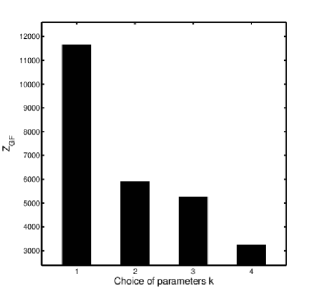
Figure 1: $Z_{GF}$ corresponding to various sets of parameters $P_{k}$ which are defined as follows. For $P_{1}$, we set each parameter to a distinct angle via $\phi_{\mathbb{j},\mu}=\pi/(j_{2}+3(j_{1}-1)+9(\mu-1))$. For $P_{2}$, we set $\phi_{\mathbb{j},\mu}=\pi/2$ for all $\mathbb{j}$ and $\mu$. For $P_{3}$, we set $\phi_{\mathbb{j},\mu}=0$ for all $\mathbb{j}$ and $\mu$. For $P_{4}$, we set $\phi_{\mathbb{j},\mu}=\pi/3+(\pi/6)(\mu-1).$

$j_{1}$	$1$	$1$	$2$	$2$	$2$	$3$	$3$	$3$
$j_{2}$	$2$	$3$	$1$	$2$	$3$	$1$	$2$	$3$
$\mu$	$1$	$1$	$1$	$1$	$1$	$1$	$1$	$1$
$\phi_{(j_{1},j_{2}),\mu}$	$-\frac{\pi}{2}$	$\frac{\pi}{5}$	$-\frac{5\pi}{11}$	$\frac{15\pi}{17}$	$-\frac{15\pi}{23}$	$\frac{28\pi}{31}$	$\frac{24\pi}{41}$	$-\frac{7\pi}{47}$

$j_{1}$	$1$	$1$	$2$	$2$	$2$	$3$	$3$	$3$
$j_{2}$	$2$	$3$	$1$	$2$	$3$	$1$	$2$	$3$
$\mu$	$2$	$2$	$2$	$2$	$2$	$2$	$2$	$2$
$\phi_{(j_{1},j_{2}),\mu}$	$\frac{2\pi}{3}$	$-\frac{5\pi}{7}$	$\frac{\pi}{13}$	$\frac{17\pi}{19}$	$\frac{27\pi}{29}$	$-\frac{\pi}{37}$	$-\frac{30\pi}{43}$	$\frac{44\pi}{53}$

Table 1: Fixed parameter values used for Figure 2.

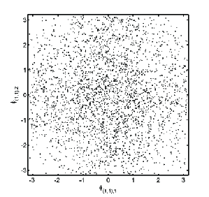
Figure 2: Subset of the discriminant locus projected onto two parameters for the $3\times 3$ lattice. The other $\phi$s are fixed as listed in Table 1. While varying $\phi_{(1,1),1}$ and $\phi_{(1,1),2}$ and leaving all other $\phi$s fixed for the $3\times 3$ lattice, the points in this plot are the points at which $Z_{GF}$ differs from the generic value $11664$.

References

- [1] R. Alkofer and L. von Smekal. The infrared behavior of QCD Green’s functions: Confinement, dynamical symmetry breaking, and hadrons as relativistic bound states. Phys. Rept., 353:281, 2001.
- [2] L. D. Faddeev and V. N. Popov. Feynman diagrams for the Yang-Mills field. Phys. Lett., B25:29–30, 1967.
- [3] C. Becchi, A. Rouet, and R. Stora. Renormalization of Gauge Theories. Annals Phys., 98:287–321, 1976.
- [4] V.N. Gribov. Quantization of non-abelian gauge theories. Nucl. Phys., B139:1, 1978.
- [5] I.M. Singer. Some Remarks on the Gribov Ambiguity. Commun. Math. Phys., 60:7–12, 1978.
- [6] H. Neuberger. Nonperturbative brs invariance. Phys. Lett., B175:69, 1986.
- [7] H. Neuberger. Nonperturbative brs invariance and the gribov problem. Phys. Lett., B183:337, 1987.
- [8] L. von Smekal, D. Mehta, A. Sternbeck, and A.G. Williams. Modified Lattice Landau Gauge. PoS, LAT2007:382, 2007.
- [9] L. von Smekal, A. Jorkowski, D. Mehta, and A. Sternbeck. Lattice Landau gauge via Stereographic Projection. PoS, CONFINEMENT8:048, 2008.
- [10] L. von Smekal. Landau Gauge QCD: Functional Methods versus Lattice Simulations. 2008.
- [11] D. Zwanziger. Local and renormalizable action from the gribov horizon. Nucl. Phys., B323:513–544, 1989.
- [12] N. Vandersickel and Daniel Zwanziger. The Gribov problem and QCD dynamics. 2012.
- [13] D. Mehta. Lattice vs. Continuum: Landau Gauge Fixing and ’t Hooft-Polyakov Monopoles. Ph.D. Thesis, 2009.
- [14] D. Mehta and M. Kastner. Stationary point analysis of the one-dimensional lattice Landau gauge fixing functional, aka random phase XY Hamiltonian. Annals Phys., 326:1425–1440, 2011.
- [15] C. Hughes, D. Mehta, and J.-I. Skullerud. Enumerating Gribov copies on the lattice. Annals Phys., 331:188–215, 2013.
- [16] D. Mehta, C. Hughes, M. Schröck, and D. J. Wales. Potential Energy Landscapes for the 2D XY Model: Minima, Transition States and Pathways. J. Chem. Phys., 139:194503, 2013.
- [17] D Mehta, C Hughes, M Kastner, and DJ Wales. Potential energy landscape of the two-dimensional xy model: Higher-index stationary points. The Journal of Chemical Physics, 140(22):224503, 2014.
- [18] D. Mehta and M. Schröck. Enumerating Copies in the First Gribov Region on the Lattice in up to four Dimensions. Phys.Rev., D89:094512, 2014.
- [19] D. Zwanziger. Fundamental modular region, Boltzmann factor and area law in lattice gauge theory. Nucl.Phys., B412:657–730, 1994.
- [20] P. van Baal. Gribov ambiguities and the fundamental domain. 1997.
- [21] M. Testa. Lattice gauge fixing, Gribov copies and BRST symmetry. Phys. Lett., B429:349–353, 1998.
- [22] A. C. Kalloniatis, L. von Smekal, and A. G. Williams. Curci-Ferrari mass and the Neuberger problem. Phys. Lett., B609:424–429, 2005.
- [23] M. Ghiotti, L. von Smekal, and A. G. Williams. Extended Double Lattice BRST, Curci-Ferrari Mass and the Neuberger Problem. AIP Conf. Proc., 892:180–182, 2007.
- [24] L. von Smekal, M. Ghiotti, and A.G. Williams. Decontracted double BRST on the lattice. Phys. Rev., D78:085016, 2008.
- [25] A. Maas. Constructing non-perturbative gauges using correlation functions. Phys.Lett., B689:107–111, 2010.
- [26] A. Maas. Describing gauge bosons at zero and finite temperature. 2011.
- [27] D. Mehta, A. Sternbeck, L. von Smekal, and A.G. Williams. Lattice Landau Gauge and Algebraic Geometry. PoS, QCD-TNT09:025, 2009.
- [28] R. Hepworth. Morse inequalities for orbifold cohomology. Algebr. Geom. Topol., 9(2):1105–1175, 2009.
- [29] M. Schaden. Equivariant gauge fixing of su(2) lattice gauge theory. Phys. Rev., D59:014508, 1999.
- [30] R. Nerattini, M. Kastner, D. Mehta, and L. Casetti. Exploring the energy landscape of XY models. Phys.Rev., E87(3):032140, 2013.
- [31] D. Birmingham, M. Blau, M. Rakowski, and G. Thompson. Topological field theory. Phys. Rept., 209:129–340, 1991.
- [32] M. Golterman and Y. Shamir. SU(N) chiral gauge theories on the lattice. Phys.Rev., D70:094506, 2004.
- [33] M. Golterman and Y. Shamir. Phase with no mass gap in nonperturbatively gauge-fixed Yang-Mills theory. Phys.Rev., D87(5):054501, 2013.
- [34] S. Catterall, D.B. Kaplan, and M. Unsal. Exact lattice supersymmetry. Phys.Rept., 484:71–130, 2009.
- [35] F. Palumbo. Gauge invariance on the lattice with noncompact gauge fields. Physics Letters B, 244(1):55–57, 1990.
- [36] C.M. Becchi and F. Palumbo. Noncompact gauge theories on a lattice: perturbative study of the scaling properties. Nuclear Physics B, 388(3):595–608, 1992.
- [37] S. Catterall, R. Galvez, A. Joseph, and D. Mehta. On the sign problem in 2D lattice super Yang-Mills. 2011.
- [38] R. Galvez, S. Catterall, A. Joseph, and D. Mehta. Investigating the sign problem for two-dimensional and lattice super Yang–Mills theories. 2012.
- [39] D. Mehta, S. Catterall, R. Galvez, and A. Joseph. Supersymmetric gauge theories on the lattice: Pfaffian phases and the Neuberger 0/0 problem. 2011.
- [40] J. Milnor. Morse theory. Based on lecture notes by M. Spivak and R. Wells. Annals of Mathematics Studies, No. 51. Princeton University Press, Princeton, N.J., 1963.
- [41] V. Guillemin and A. Pollack. Differential topology. Prentice-Hall Inc., Englewood Cliffs, N.J., 1974.
- [42] Private communication with L. von Smekal.
- [43] A. Adem, J. Leida, and Y. Ruan. Orbifolds and stringy topology, volume 171 of Cambridge Tracts in Mathematics. Cambridge University Press, Cambridge, 2007.
- [44] I. Satake. The Gauss-Bonnet theorem for -manifolds. J. Math. Soc. Japan, 9:464–492, 1957.
- [45] W.P. Thurston. Three-dimensional geometry and topology. Vol. 1, volume 35 of Princeton Mathematical Series. Princeton University Press, Princeton, NJ, 1997. Edited by Silvio Levy.
- [46] M. Boileau, S. Maillot, and J. Porti. Three-dimensional orbifolds and their geometric structures, volume 15 of Panoramas et Synthèses [Panoramas and Syntheses]. Société Mathématique de France, Paris, 2003.
- [47] L.J. Dixon, J.A. Harvey, C. Vafa, and E. Witten. Strings on Orbifolds. Nucl. Phys., B261:678–686, 1985.
- [48] L.J. Dixon, J.A. Harvey, C. Vafa, and E. Witten. Strings on Orbifolds. 2. Nucl. Phys., B274:285–314, 1986.
- [49] S.-S. Roan. Minimal resolutions of Gorenstein orbifolds in dimension three. Topology, 35(2):489–508, 1996.
- [50] A. Adem and Y. Ruan. Twisted orbifold -theory. Comm. Math. Phys., 237(3):533–556, 2003.
- [51] M. Atiyah and G. Segal. On equivariant Euler characteristics. J. Geom. Phys., 6(4):671–677, 1989.
- [52] J. Bryan and J. Fulman. Orbifold Euler characteristics and the number of commuting -tuples in the symmetric groups. Ann. Comb., 2(1):1–6, 1998.
- [53] H. Tamanoi. Generalized orbifold Euler characteristic of symmetric products and equivariant Morava -theory. Algebr. Geom. Topol., 1:115–141 (electronic), 2001.
- [54] H. Tamanoi. Generalized orbifold Euler characteristics of symmetric orbifolds and covering spaces. Algebr. Geom. Topol., 3:791–856 (electronic), 2003.
- [55] C. Farsi and C. Seaton. Generalized orbifold Euler characteristics for general orbifolds and wreath products. Algebr. Geom. Topol., 11(1):523–551, 2011.
- [56] A.J. Sommese and C.W. Wampler. The numerical solution of systems of polynomials arising in Engineering and Science. World Scientific Publishing Company, 2005.
- [57] D.J. Bates, J.D. Hauenstein, A.J. Sommese, and C.W. Wampler. Numerically solving polynomial systems with Bertini, volume 25. SIAM, 2013.
- [58] D. Mehta. Numerical Polynomial Homotopy Continuation Method and String Vacua. Adv.High Energy Phys., 2011:263937, 2011.
- [59] M. Maniatis and D. Mehta. Minimizing Higgs Potentials via Numerical Polynomial Homotopy Continuation. Eur.Phys.J.Plus, 127:91, 2012.
- [60] M. Kastner and D. Mehta. Phase Transitions Detached from Stationary Points of the Energy Landscape. Phys.Rev.Lett., 107:160602, 2011.
- [61] D. Mehta, Y. H. He, and J. D. Hauenstein. Numerical Algebraic Geometry: A New Perspective on String and Gauge Theories. JHEP, 1207:018, 2012.
- [62] D. Mehta, J. D. Hauenstein, and M. Kastner. Energy landscape analysis of the two-dimensional nearest-neighbor model. Phys.Rev., E85:061103, 2012.
- [63] J. Hauenstein, Y. H. He, and D. Mehta. Numerical elimination and moduli space of vacua. JHEP, 1309:083, 2013.
- [64] B. Greene, D. Kagan, A. Masoumi, D. Mehta, E. J. Weinberg, and X. Xiao. Tumbling through a landscape: Evidence of instabilities in high-dimensional moduli spaces. Phys.Rev., D88(2):026005, 2013.
- [65] D. Mehta, D. A. Stariolo, and M. Kastner. Energy landscape of the finite-size spherical three-spin glass model. Phys.Rev., E87(5):052143, 2013.
- [66] D. Martinez-Pedrera, D. Mehta, M. Rummel, and A. Westphal. Finding all flux vacua in an explicit example. JHEP, 1306:110, 2013.
- [67] Y. H. He, D. Mehta, M. Niemerg, M. Rummel, and A. Valeanu. Exploring the Potential Energy Landscape Over a Large Parameter-Space. JHEP, 1307:050, 2013.
- [68] J.D. Hauenstein, A.J. Sommese, and C.W. Wampler. Regeneration homotopies for solving systems of polynomials. Mathematics of Computation, 80(273):345–377, 2011.
- [69] D.J. Bates, J.D. Hauenstein, A.J. Sommese, and C.W. Wampler. Bertini: Software for numerical algebraic geometry. Available at http://bertini.nd.edu.