Main Belt Asteroids with WISE/NEOWISE: Near-Infrared Albedos

Abstract

We present revised near-infrared albedo fits of $2835$ Main Belt asteroids observed by WISE/NEOWISE over the course of its fully cryogenic survey in 2010. These fits are derived from reflected-light near-infrared images taken simultaneously with thermal emission measurements, allowing for more accurate measurements of the near-infrared albedos than is possible for visible albedo measurements. As our sample requires reflected light measurements, it undersamples small, low albedo asteroids, as well as those with blue spectral slopes across the wavelengths investigated. We find that the Main Belt separates into three distinct groups of $6\%$, $16\%$, and $40\%$ reflectance at $3.4~{}\mu$m. Conversely, the $4.6~{}\mu$m albedo distribution spans the full range of possible values with no clear grouping. Asteroid families show a narrow distribution of $3.4~{}\mu$m albedos within each family that map to one of the three observed groupings, with the (221) Eos family being the sole family associated with the $16\%$ reflectance $3.4~{}\mu$m albedo group. We show that near-infrared albedos derived from simultaneous thermal emission and reflected light measurements are an important indicator of asteroid taxonomy and can identify interesting targets for spectroscopic followup.

1 Introduction

The Wide-field Infrared Survey Explorer (WISE, Wright et al., 2010) performed an all-sky survey in the thermal infrared, imaging each field of view simultaneously in four infrared wavelengths during the fully cryogenic portion of the mission and in the two shortest wavelengths when the mission continued as the Near-Earth Object WISE survey (NEOWISE, Mainzer et al., 2011a). The four WISE bandpasses are referred to as W1, W2, W3, and W4, and cover the wavelength ranges of $3.1-3.8~{}\mu$m, $4.1-5.2~{}\mu$m, $7.6-16.3~{}\mu$m, and $19.8-23.4~{}\mu$m respectively, with photometric central wavelengths of $3.4~{}\mu$m, $4.6~{}\mu$m, $12~{}\mu$m, and $22~{}\mu$m respectively (Wright et al., 2010).

The single-frame WISE/NEOWISE data allow us to investigate the thermal emission and reflectance properties of the minor planets of the Solar system. Due to their proximity to the Sun, near-Earth objects (objects with perihelia $q<1.3~{}$AU) are typically dominated by thermal emission in W2 (and occasionally even in W1), while for more distant objects W2 measures a combination of reflected and emitted light and W1 is dominated by reflected light. For all minor planets observed by NEOWISE, bands W3 and W4 are dominated by thermal emission.

Measurements of the thermal emission from asteroids can be used to determine the diameter of these bodies through the application of thermal models such as the Near Earth Asteroid Thermal Model (NEATM, Harris, 1998). NEATM assumes that the asteroid is a non-rotating sphere with no emission from the night side, and a variable beaming parameter ($\eta$) is used to account for variability in thermophysical properties and phase effects. NEATM provides a rapid method of determining diameter from thermal emission data that is reliable to $\sim 10\%$ when the beaming parameter can be fit (Mainzer et al., 2011b). Visible light measurements available from the Minor Planet Center (MPC) can then be combined with these models to constrain the geometric albedo at visible wavelengths ($p_{V}$). However, as these data are not simultaneous with the thermal infrared measurements, uncertainties due to rotation phase, observing geometry, and photometric phase behavior instill significant systematic errors in $p_{V}$ determinations. The preliminary asteroid thermal fits presented in Mainzer et al. (2011e, 2012); Masiero et al. (2011, 2012a); Grav et al. (2011a, b) for the near-Earth objects, Main Belt asteroids, Hildas, and Jupiter Trojans account for these uncertainties in the determination of the optical $H$ magnitude resulting in a larger relative error on albedo than is found for diameter.

For objects that were observed by NEOWISE in both thermal emission and near-infrared (NIR) reflected light, we can simultaneously constrain the diameter as well as the NIR albedo. As these data were taken at the same time and observing conditions as the thermal data used to model the diameter, no assumptions are needed regarding the photometric phase behavior of these objects, and light curve changes from rotation or viewing geometry do not contribute to the uncertainty. These NIR albedos will thus be a more precise indicator of the surface properties than the visible albedos.

The behavior of the NIR region of an asteroid’s reflectance spectrum can be used as a probe of the composition of the surface. Spectra of asteroids in the NIR have been used for taxonomic classification (DeMeo et al., 2009), to constrain surface mineralogy (Gaffey et al., 2002; Reddy et al., 2012a), and to search for water in the Solar system (Rivkin & Emery, 2010; Campins et al., 2010). Near-infrared albedo measurements have also been used to identify candidate metal-rich objects in the NEO population (Harris & Drube, 2014). Mainzer et al. (2011d) use the ratio of the NIR and visible albedos as a proxy for spectral slope, and show a correspondence between this ratio and various taxonomic classifications. This relation was used by Mainzer et al. (2011e) to determine preliminary classifications for NEOs, while Grav et al. (2011b) and Grav et al. (2012) expanded upon this technique to taxonomically classify Hilda and Jupiter Trojan asteroids.

Masiero et al. (2011) presented NIR albedo measurements of Main Belt asteroids assuming that the albedos at the W1 and W2 wavelengths were identical. However, for objects that have a sufficient number of detections of reflected light in multiple NIR bands we can independently constrain each albedo ($p_{W1}$ and $p_{W2}$ for the W1 and W2 bandpasses respectively). In this work, we present new thermal model fits of the NIR albedos of Main Belt asteroids (MBAs), allowing $p_{W1}$ and $p_{W2}$ to vary independently. These albedos allow us to better distinguish different MBA compositional classes. They are also particularly useful for investigations of collisional families seen in the Main Belt, which show strongly correlated physical properties within each family.

2 Data and Revised Thermal Fits

To fit for NIR albedos of Main Belt asteroids, we use data from WISE/NEOWISE all-sky single exposure source table, which are available for download from the Infrared Science Archive (IRSA Cutri et al., 2012). We extract photometric measurements of all asteroids observed by WISE following the technique described in Masiero et al. (2011) and Mainzer et al. (2011a). In particular, we use the NEOWISE observations reported to the MPC and included in the MPC’s minor planet observation database as the final validated list of reliable NEOWISE detections of Solar system objects.

For objects with WISE detections in all four bands, we follow the fitting technique described in Grav et al. (2012) to independently determine the albedos in bands W1 and W2. This technique uses a faceted sphere with a temperature distribution drawn from the NEATM model to calculate the predicted visible and infrared magnitudes for each object. Diameter, beaming parameter, and visible, W1, and W2 albedos are all varied until a best-fit is found. Monte carlo simulations of the data using the measurement errors then provide a constraint on the uncertainty of each parameter. We require at least three detections in each band above SNR=4 to use that band in our fit. Main Belt asteroids are typically closer to the Sun at the time of observation than the Trojans and Hildas discussed in Grav et al. (2012), and thus the measured W2 flux can have a larger contribution of thermal emission for MBAs. Flux in the W1 band is typically dominated by reflected light for MBAs observed by WISE, although low albedo objects ($p_{V}<0.1$) at heliocentric distances of $R_{\sun}<2.5~{}$AU can be thermally dominated in W1 as well.

In order to ensure reliable fits for W2 albedos ($p_{W2}$), we require that the beaming parameter be fit by the model. The beaming parameter is a variable in the NEATM fit that consolidates uncertainties in the model due to viewing geometries and surface thermophysical parameters, and can be characterized as an enhancement of the thermal emission in the direction of the Sun. Changes in thermal properties or phase angles will lead to a range of possible beaming parameters for MBAs. In order to fit the beaming parameter, our model requires detections of thermal emission in two bands. We also require that the fraction of flux in W2 from reflected light be at least $10\%$ of the total flux measured to fit $p_{W2}$. While this should be sufficient to constrain the W2 albedo in most cases, uncertainty in the beaming parameter can lead to large uncertainties in $p_{W2}$. To fit W1 albedo ($p_{W1}$), we followed the same procedure for $p_{W2}$, except now requiring the W1 reflected light to be at least $50\%$ of the total flux. All objects that fulfilled the above requirements had optically measured magnitudes available in the literature, and thus allowed us to fit a visible albedo as well.

We present our updated thermal model fits for all objects satisfying the above constraints in Table 1, where we give the object’s name in MPC-packed format, absolute $H_{V}$ magnitude and $G$ photometric slope parameter from the MPC orbit file, associated family from Masiero et al. (2013) (or “…” if the object is not associated to a family), and our best fit and associated uncertainty on diameter, beaming parameter ($\eta$), $p_{W1}$, and $p_{W2}$ if the latter could be constrained (“…” otherwise). Objects with two epochs of coverage have each epoch listed separately. All errors are statistical and do not include the systematic errors of $\sim 10\%$ on diameter and $\sim 20\%$ on visible albedo (cf. Mainzer et al., 2011b, c; Masiero et al., 2011). Systematic errors will increase the absolute error on the fitted quantities, but do not affect relative comparisons within our sample, which is the main goal of this paper. This table contains $3080$ fits of $2835$ unique objects: $709$ fits of $679$ unique objects with constrained $p_{W1}$ and $p_{W2}$; $2371$ fits of $2219$ unique objects with only $p_{W1}$ constrained; $63$ objects that had one epoch where both NIR albedos were constrained and one epoch where only $p_{W1}$ could be fit.

We note that some of the fits for diameter and beaming parameter (and thus albedo) are different from those presented in Masiero et al. (2011). Fits from NEATM using the same data set will give different values for the diameter as the beaming parameter is varied. In this case, by independently considering $p_{W1}$ and $p_{W2}$, as opposed to averaging over both for a single value of $p_{IR}$, the calculated contribution of thermal flux in W2 will vary, which will result in a refined value of $\eta$ and therefore diameter. For the majority of cases, diameters are consistent to within $10\%$ of the previous value, visible albedos are consistent within $20\%$, and infrared albedo and beaming parameters are consistent within $15\%$. Revised beaming parameters tend to be $\sim 5\%$ smaller, making diameters $\sim 3\%$ smaller and visible albedos $\sim 6\%$ larger. W1 infrared albedos tend to increase $\sim 8\%$, however we are not necessarily comparing similar quantities as the previous fits assumed W1 and W2 albedos were equal, allowing W2 measurements to alter the best-fit value.

Table 1: Revised thermal fits of Main Belt asteroids. Table 1 is published in its entirety in the electronic edition; a portion is shown here for guidance regarding its form and content

Name	diameter (km)	$\eta$	$p_{V}$	$p_{W1}$	$p_{W2}$	$H_{V}$	G	Family
00005	108.29$\pm$ 3.70	0.87$\pm$0.10	0.27$\pm$0.03	0.37$\pm$0.03	0.20$\pm$0.10	6.9	0.15	00005
00006	195.64$\pm$ 5.44	0.91$\pm$0.09	0.24$\pm$0.04	0.35$\pm$0.03	0.48$\pm$0.32	5.7	0.24	…
00008	147.49$\pm$ 1.03	0.81$\pm$0.01	0.23$\pm$0.04	0.38$\pm$0.04	…	6.4	0.28	00008
00009	183.01$\pm$ 0.39	0.86$\pm$0.01	0.16$\pm$0.03	0.33$\pm$0.01	…	6.3	0.17	…
00009	184.16$\pm$ 0.90	0.78$\pm$0.01	0.16$\pm$0.01	0.34$\pm$0.04	…	6.3	0.17	…
00011	142.89$\pm$ 1.01	0.78$\pm$0.02	0.19$\pm$0.02	0.35$\pm$0.03	…	6.6	0.15	…
00012	115.09$\pm$ 1.20	0.84$\pm$0.02	0.16$\pm$0.03	0.32$\pm$0.02	…	7.3	0.22	00012
00014	140.76$\pm$ 8.41	0.84$\pm$0.15	0.27$\pm$0.04	0.39$\pm$0.06	0.19$\pm$0.16	6.3	0.15	…
00015	231.69$\pm$ 2.23	0.79$\pm$0.04	0.25$\pm$0.04	0.40$\pm$0.04	…	5.3	0.23	00015
00017	84.90$\pm$ 2.03	0.77$\pm$0.04	0.19$\pm$0.03	0.37$\pm$0.08	…	7.8	0.15	…

The criteria we apply to our fits, discussed above, result in selection effects in our sample that conspire to under-represent the lowest albedo asteroids, as these objects are more likely to fall below our detectability threshold. This bias is a fundamental result of requiring reflected light observations in W1 and/or W2, but does not affect population surveys based on emission in W3 or W4. Our sample requirements also drive us to only use the data from the fully cryogenic portion of the WISE survey. It is possible to use fully cryogenic data to constrain the diameter and beaming parameter, and later measurements from either the NEOWISE post-cryo survey or the recently restarted NEOWISE mission (Mainzer et al., 2014) during a brighter apparition to constrain the NIR albedo properties (cf. Grav et al., 2012), although this technique requires a different method of handling that addresses difference in viewing geometry. We will apply this technique to Main Belt asteroids in future work.

For objects with a sufficient number of detections in W1 but below our W2 sensitivity limit or our threshold for the fraction of reflected light in W2, we determine only the W1 albedo. These objects are either too small to reflect a detectable amount of light in W2, may be dominated by thermal emission in W2 (common for low albedo objects, $p_{W1}<0.1$), or may have a blue spectral slope over the $3-5~{}\mu$m range and thus “drop out” of W2. Each of these scenarios will have a different implication for interpreting the distribution of W2 albedos, most notably that our data are least sensitive to smaller, lower albedo objects, as well as objects with blue $p_{V}$-$p_{W2}$ or $p_{W1}$-$p_{W2}$ spectral slopes. Interpretation of the distribution of NIR albedos or spectral slopes, particularly as a function of taxonomy or size, must thus be made with the appropriate caveats. We also explore stacking of the predicted positions of these object in W2 to recover drop-out objects in future work.

3 Discussion

3.1 Albedo comparisons

Figure 1 shows $p_{W1}$ and $p_{W2}$ for all Main Belt asteroids with sufficient data to constrain these parameters, compared to the fitted diameter. The W1 band is more sensitive than the W2 band (single-frame $5\sigma$ sensitivity of $\sim 0.22~{}$mJy vs $\sim 0.31~{}$mJy respectively, Cutri et al., 2012), and W1 detections are less frequently contaminated by thermal emission, meaning we are able to measure $p_{W1}$ for more asteroids than have $p_{W2}$ measurements ($2835$ vs $679$). Both data sets show a strong bias against small, low-albedo asteroids, as is expected for data that require measurement of a reflected light component. A further bias against dark objects in $p_{W2}$ due to rising thermal emission overtaking the small reflected light component is also present. From the data available we see no evidence for a non-uniform distribution of $p_{W2}$, in contrast to $p_{W1}$ which shows three significant albedo clumps at $p_{W1}\sim 0.06$, $p_{W1}\sim 0.16$, and $p_{W1}\sim 0.4$.

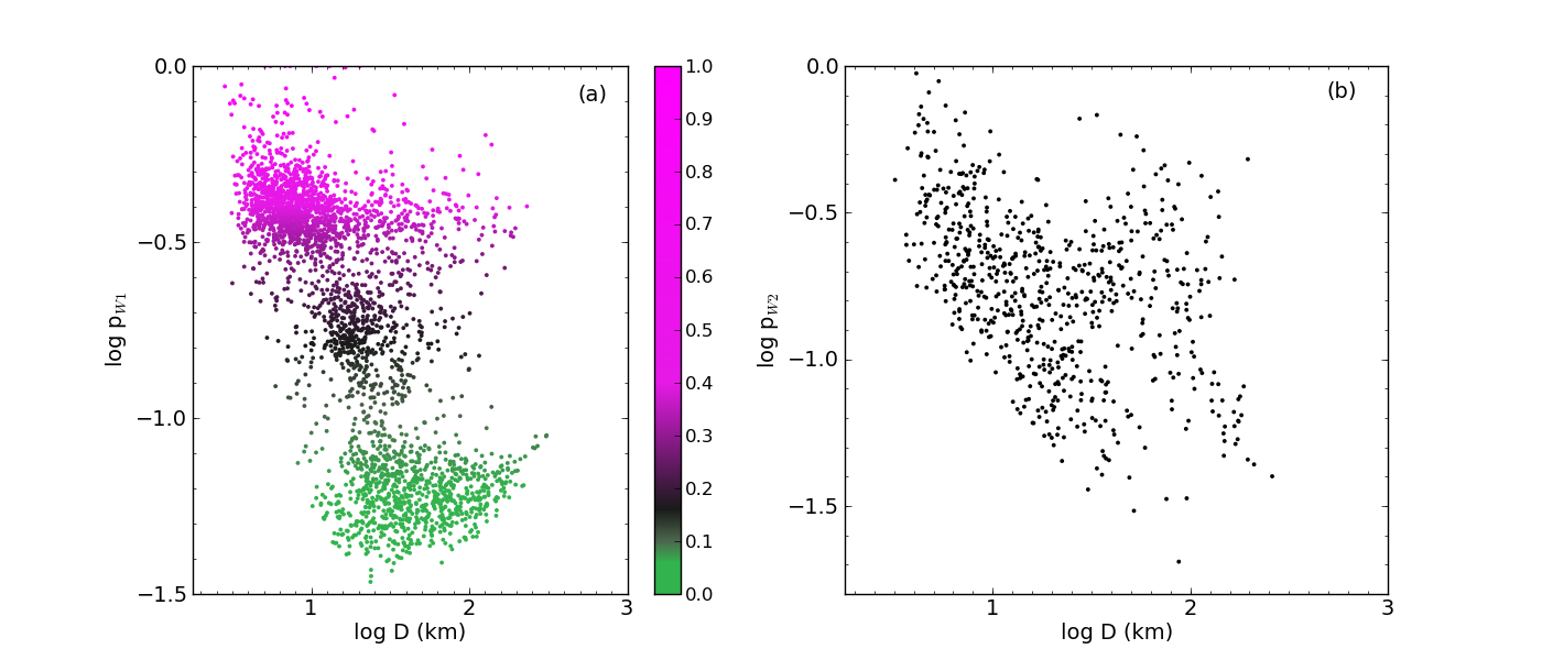
Figure 1: (a) W1 infrared albedo ($p_{W1}$) compared to fitted diameter, where color also indicates $p_{W1}$ (as used in Figure 7). (b) W2 infrared albedo ($p_{W2}$) compared to diameter. As the W1 and W2 detections are a measurement of reflected light they are strongly biased by albedo. The dearth of small, low albedo objects in this plot that are observed in Masiero et al. (2011) is an artifact of this bias.

Visible albedos for over $136,000$ Main Belt asteroids were presented in Masiero et al. (2011) and Masiero et al. (2012a). These measurements were based on the conversion of apparent visible magnitudes from a wide range of predominantly ground-based surveys to absolute $H_{V}$ magnitudes when the orbit was determined by the MPC. Absolute magnitude is then converted to a predicted apparent magnitude during the epoch of the WISE/NEOWISE observations, often after assuming a photometric $G$ parameter (cf. Bowell et al., 1989) and assuming rotational variations are averaged over during the set of thermal infrared observations. These conversions and assumptions will instill additional uncertainty in the $p_{V}$ determinations beyond what would be expected from uncertainties in the flux measurements and from thermal modeling. As a result, the fractional error on $p_{V}$ is typically $50-100\%$ larger than the fractional error on diameter from thermal model fits.

We compare the NIR albedos presented here to these visible albedos in Figures 2 and 3. For the majority of objects, $p_{W1}$ traces $p_{V}$ and can thus be used as an analog when $p_{V}$ is not available. The uncertainties of the $p_{W1}$ measurements in our data are smaller than the errors on $p_{V}$, and thus act as a better constraint of the surface properties. The relationship between $p_{W2}$ and both $p_{V}$ and $p_{W1}$ is less distinct, and varies over a large range of values for objects spanning high and low $p_{V}$ and $p_{W1}$ albedos.

Comparing the $p_{V}$ distribution to Figure 10 from Masiero et al. (2011), we see that our sample contains significantly fewer low albedo objects than would be expected from a random sample of all Main Belt asteroids. The lack of low albedo objects is due primarily to the observational selection effect imprinted on our dataset by the requirement that the objects be detected in W1 and/or W2 in reflected light. This bias will increase as albedo decreases, preferentially selecting objects with higher albedos. A survey with deeper sensitivity in these wavelengths would allow us to probe smaller sizes at all albedos, but would still be subject to the same observational biases.

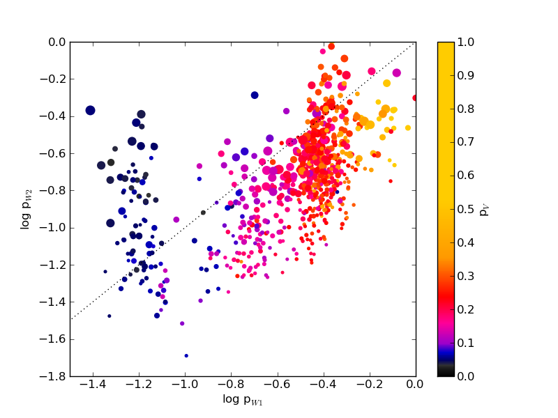
Figure 2: W2 albedo vs W1 albedo for $679$ Main Belt asteroids. The color of the points indicate their visible albedo following the colormap presented in Masiero et al. (2011) and shown in the colorbar, while the size of the point traces the fraction of the W2 flux that was due to reflected light. The dotted line shows a 1-to-1 correspondence; objects below the line will have a blue spectral slope from W1 to W2, while objects above the line will have a red slope.

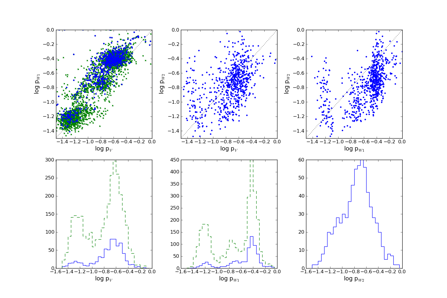
Figure 3: Comparisons (top) and histograms (bottom) of asteroid albedos at visible ($p_{V}$), W1 ($p_{W1}$), and W2 ($p_{W2}$) wavelengths. Blue points/lines show objects with all three albedos fit by the thermal model ($679$ objects), while green crosses/dashed lines show objects with only visible and W1 fits ($2835$ objects). Plots of $p_{W2}$ do not include green crosses as these objects do not have this parameter constrained by the model fits. Dotted black lines in the comparison plots indicate a 1-to-1 relation. While visible and W1 albedos show clear clumping, W2 albedos show no separation within our measurement errors.

Following Grav et al. (2012), we can use our albedo measurements as a proxy for spectral slope from visible wavelengths through the NIR. Objects that fall above the 1-to-1 relationship in the top portion of Figure 3 will have a red spectral slope across the wavelengths plotted, while objects below this relation will have a blue spectral slope. As $p_{W2}$ is the most poorly probed of the three parameters, there will be inherent detection biases against blue spectral slopes from objects that “drop out” and fall below our W2 detection threshold. For this reason objects with the bluest slopes, particularly low-albedo objects, will be under-represented in our fits of $p_{W2}$.

To better compare the spectral slope information, in Figure 4 we show the difference in albedo between $p_{V}$, $p_{W1}$, and $p_{W2}$ normalized to the measured $p_{W1}$ value. Objects with positive values have a red spectral slope, while objects with negative values have a blue slope. High albedo objects ($p_{W1}>0.1$) tend to show red slopes from visible to W1 wavelengths, and then blue slopes between W1 and W2. This behavior is similar to what is observed for Eucrite meteorites at these wavelengths (Reddy et al., 2012b), and what would be expected from extrapolating a typical S-type asteroid spectrum (DeMeo et al., 2009). High albedo objects without a measured $p_{W2}$ albedo show similar visible-W1 slopes to those with a measured $p_{W2}$.

Low albedo objects ($p_{W1}<0.1$) behave quite differently from their high-albedo counterparts. While slightly red from the visible to W1, these objects show a wide range of visible-W2 and W1-W2 slopes, from neutral in color to very red. An important caveat to this is shown by the objects without $p_{W2}$ fits, which have slopes ranging from moderately red to significantly blue. Blue-sloped objects would be much fainter in W2 than W1 and thus would drop out from detection or be dominated by thermal emission in W2. It is probable that there is a population of these objects with blue W1-W2 slopes that are not represented in our plots. Extrapolting from the NIR spectra of low albedo objects from DeMeo et al. (2009), we associate our objects that have red visible-W1 slopes with C-type and D-type objects. We can similarly associate the objects having blue-slopes with B-type asteroids, however we note that only $\sim 1\%$ of objects studied by DeMeo et al. (2009) were identified as B-type asteroids, while $\sim 10\%$ of the asteroids in our study have low albedo and blue spectral slope. From Neese (2010) we find that the majority of our blue sloped objects that have Bus-DeMeo taxonomic classifications are identified as B or Ch class objects, the latter of which represents a fraction of the spectroscopic sample comparable to the fraction of our sample in this group. Our blue slope may be indicative of the presence of mineralogical absorption features in the spectra of low albedo objects at the wavelengths covered by W1.

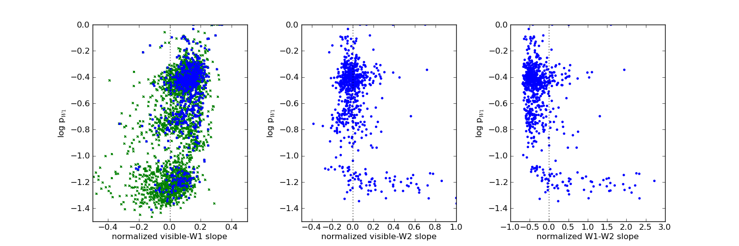
Figure 4: Spectral slope, normalized to the W1 albedo, over visible-to-W1 wavelengths (left), visible-to-W2 wavelengths (center) and W1-to-W2 wavelengths (right), compared to the W1 albedo. The dotted line shows a neutral slope; objects with positive slope values have red spectra and objects with negative values have blue spectra. High albedo objects tend to be red-sloped from visible to W1, and blue sloped from W1 to W2, while low albedo objects tend to be flat or red across the whole range. Color/shape of points is the same as used in Figure 3.

3.2 D-type asteroids

Asteroids with D-type taxonomic classifications become increasingly common as distance from the Sun grows, from the Main Belt through the Jupiter Trojan population (DeMeo & Carry, 2013). These objects, especially the Jupiter Trojans, were likely implanted from a more distant reservior during the early chaotic evolution of the Solar system (Morbidelli et al., 2005) and thus represent primitive material distinct from objects that formed in the warmer region of the Main Belt. NIR albedo can be used to probe the distribution of these objects and differentiate between classes of primitive bodies. Grav et al. (2012) compare $p_{W1}$ and $p_{W2}$ to distinguish asteroids with D-type taxonomic classification from those with C- and P-type, and are able to determine the overall population fraction of D-type objects in the Jupiter Trojan and Hilda populations. They find that the majority of Jupiter Trojans are D-type at all sizes, while the Hilda population transitions from a minority of D-types at diameters $D>40~{}$km to a majority at smaller sizes.

Following Grav et al. (2012), we show in Figure 5 an expanded view of the objects with lowest infrared albedos. We highlight the region of albedo-space that is occupied by D-type asteroids in the Trojan and Hilda populations. The diameter and albedo fits from Grav et al. (2012) rely on the same model and assumptions as we use here, and so comparisons between the two populations should only depend on the random error associated with the fits. Only $2\%$ of all objects for which we measure $p_{W1}$ and $p_{W2}$ fall in this region; with the exception of (114) Kassandra and (267) Tirza (which are spectrally classified as T- and D-type objects, respectively), all other candidate D-type objects are in the outer Main Belt and have diameters between $10~{}$km$<D<40~{}$km, consistent with the diameter regime where D-types dominate the Hilda asteroids. One object, (1755) Lorbach, is identified as an S-type in Neese (2010), but this classification relies on only two optical colors. For the outer Main Belt, we do not see a significant population of D-type objects like what is observed in the Hildas and Trojans (DeMeo & Carry, 2013), but this is expected from the lower efficiency of dynamical implantation compared with the Hilda and Trojan populations Levison et al. (2009).

We find no objects in the inner Main Belt with albedos consistent with D-type objects. This is in contrast to the results of DeMeo et al. (2014) who find a small population of these bodies; however, this difference can be understood through the selection effects in our survey. Although our sample probes a large number of objects with semimajor axis $a<2.5~{}$AU only a handful have low albedo. Inner Main Belt low albedo asteroids are more likely to have significant thermal emission in W2, so we are not able to determine $p_{W2}$ for these objects and they will not appear in our analysis.

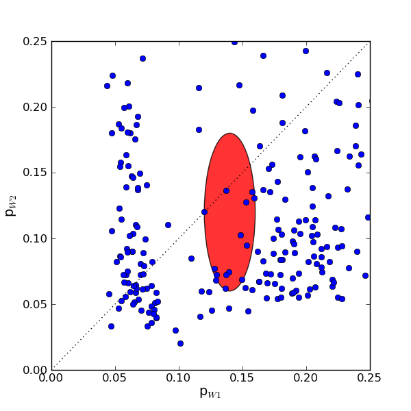
Figure 5: W1 and W2 albedos for all measured objects. The red ellipse marks the region populated by D-type asteroids as identified in Grav et al. (2012). This taxonomic classification shows no significant representation in the Main Belt objects studied here.

3.3 Low-$p_{W1}$/High-$p_{W2}$ objects

Figure 5 shows a group of objects with low visible and W1 albedos ($p_{V},p_{W1}<0.1$) but high W2 albedo ($p_{W2}>0.1$), which also appear as the objects with the reddest W1-W2 slopes in Figure 4. This class of object does not have an analog in the Jupiter Trojan or Hilda populations (Grav et al., 2012) where we find parallels to other low-albedo MBA populations. Objects from this group that have spectroscopic or photometric taxonomic classifications in PDS are typically designated as C-type or a related subclass (Neese, 2010). There are occasional objects with other classifications such as X-, F- and S-, or dual classifications, although often in these cases the designation is based on only 2 color indices and so is of low reliability. It is possible that this group could represent a different class of objects that is not found in the more distant Solar system populations, or instead could be a failure of the thermal model to converge for certain objects with low albedos.

In order to test if these objects are a result of a failure of the fitting routine, we take all objects in our fitted population with $p_{W1}<0.1$ and compare the set with $p_{W2}\geq 0.1$ to the set with $p_{W2}<0.1$ (referred to as “low-high” and “low-low” respectively). The low-high and low-low test sets are approximately the same size (44 vs 48 objects), and have similar distributions of semimajor axes, eccentricities, inclinations, $p_{V}$ and $p_{W1}$. The primary difference between these two groups is that the low-high objects have significantly smaller heliocentric distances at the time of observation than the low-low objects, resulting in higher subsolar temperatures. The diameters of the low-high objects are also characteristically smaller than those of the low-low group, however we cannot distinguish if this is an actual difference between the groups or is a change in sensitivity as a result of the low-high objects being closer to the Sun and telescope at the time of observation, and thus warmer and brighter.

The asteroid (656) Beagle is a particularly interesting case for testing the differences between these two sets of objects. NEOWISE observed this asteroid at two different epochs, both while fully cryogenic, with good sensitivity at all four bands. One epoch of observations results in a NEATM best-fit that falls into the low-low group, while the other epoch falls into the low-high group. The low-high epoch data were taken when Beagle was $0.21~{}$ AU closer to the Sun ($2.82~{}$AU vs $3.03~{}$AU for the low-low case), following the trend seen for the overall population. The best-fit for NEATM in the low-high epoch has a beaming parameter of $\eta=1.46$ and a diameter of $D=62~{}$km while the low-low epoch has best-fit values of $\eta=1.03$ and $D=48~{}$km which is the reverse of the diameter trend mentioned above. This large disagreement in diameter is not unexpected given the difference in best-fit beaming parameter which is inversely proportional to the fourth power of the subsolar temperature used in the NEATM model, and thus will change the model’s emitted flux.

The observations used for our fits were visually inspected, as well as compared to the WISE all-sky atlas of stationary sources, and show no significant contamination by background stars or galaxies. We note that (656) Beagle has a large amplitude lightcurve (A$>1~{}$mag) and a period of $7.035~{}$hours (Menke, 2005). Although large amplitudes can increase uncertainty in the fits, our data consist of 12 data points over $1$ day and 15 data points over $1.25$ days, so both epochs cover multiple rotations. As such, light curve variations should be averaged over by our fits, and should only contribute a small amount to the total uncertainty in the fit.

As a test of our model, we perform a NEATM fit using only bands W1, W2, and W3 as constraints, assuming the W4 measurements are anomalously high, and a fixed beaming parameter of $\eta=1.0$. When using a fixed beaming parameter we cannot adequately constrain $p_{W2}$, and so assume it is equal to $p_{W1}$. For these restricted fits, both epochs converge to diameters that agree to within $10\%$, but they cannot reproduce the measured magnitudes as well as the full-fit case. As we are using one fewer constraint but two fewer variables, this is not surprising. The fits for (656) Beagle given by Masiero et al. (2011) are nearly identical to these restricted fits, but also cannot fully reproduce the measured magnitudes, particularly for the low-high epoch. Restricting our model further and only fitting W1 and W3, we find that both epochs converge to nearly identical diameters, and visible and infrared albedos.

We can understand these results by looking at where the best-fit model deviates from the data. For the low-high epoch, the full NEATM fit cannot reproduce the W2, W3, and W4 fluxes simultaneously, with the W2 and W4 measurements showing excesses not observed in W3. Our full model finds a best fit solution allowing W3 and W4 to determine the diameter and beaming which under-produces flux in W2, but corrects that by increasing $p_{W2}$. If we ignore the W4 measurements, the W2 and W3 fluxes still cannot be reproduced in the low-high epoch solely with thermal emission and reflected light without resorting to extreme changes in $p_{W2}$.

One possible explanation for the disagreement between epochs is that we are observing significant differences between the thermal emission in the morning and afternoon hemispheres of the asteroid. If (656) Beagle has a relatively high thermal inertia, there may be a significant lag to the thermal re-emission of incident light which is not accounted for in the NEATM model. Our two epochs of observation are at phase angles of $\alpha\sim 20^{\circ}$, but on opposite sides of the body. (656) Beagle is on a low-inclination orbit, so if we assume the rotation pole is oriented perpendicular to the orbital and ecliptic planes and that the rotation is prograde, then the data from the low-high epoch would correspond to the afternoon hemisphere and the data from the low-low epoch would correspond to the morning hemisphere. Future work will implement a full thermophysical model of this object to test if the W2 and W4 excesses can be explained by a morning/afternoon dichotomy. For all other objects in the low-high group which were only observed at a single epoch, we cannot currently differentiate between poor fits to the beaming parameter and actual excesses in the W2 and/or W4 bands.

An alternate possibility is that these fits are indicative of problems with the flux measurement of partially saturated sources in the WISE data. Cutri et al. (2012) discuss the process by which fluxes are measured for saturated sources through PSF-fitting photometry. Flux measurements are available for sources many magnitudes above the brightness where the central pixel saturates through fitting of the PSF wings, however for very bright sources in bands W2 and W3, there appears to be a slight over-estimation of the fluxes. None of the objects we fit here had W2 magnitudes in this saturated regime, however the majority of objects with $p_{W1}<0.1$ had W3 magnitudes in this problematic region.

We correct for saturation estimation issues in our thermal model, however there is the potential that the error for asteroidal sources cannot be adequately described by this correction, which was calibrated for stars. The difference in the spectral energy distributions through the W3 bandpass of hot, blue stars and cooler, red asteroids potentially could result in differences deep in the wings of the PSF for each type of source that are not fully encompassed by the color correction. These subtle changes can have a significant impact on saturated sources where only the wings are available for profile-fitting, however there are an insufficient number of well-calibrated, W3-bright sources with the appropriate spectral energy distribution to correct for this effect. Although this error may only have a small effect on other physical parameters within our modeled systematic uncertainties, due to W2’s position on the Wien’s side of Main Belt asteroid thermal emission for some of our objects, a small change in W3 can result in a large change in W2 flux, and thus our interpretation of the W2 albedo. As such, caution is strongly encouraged in interpreting fits for objects with very bright W3 magnitudes (W3$<4~{}$mag).

3.4 NIR Albedos of Asteroid Families

The distributions of visible albedos for members of each asteroid family have much narrower spread than the albedo distribution of the Main Belt as a whole (Masiero et al., 2011) as is expected from a population resulting from the collisional breakup of a single parent body. As the (4) Vesta family shows a narrow albedo distribution but originated from a differentiated body, we do not expect the albedo distributions of other cratering-event families that may have been partially- or fully-melted to differ significantly from non-differentiated families. It is possible that families formed from the complete disruption of a differentiated parent body may show a broader albedo distribution, though we do not see any evidence for a case like this in our data. Visible albedo can also be used to improve family membership lists by rejecting outlier objects that are dynamically similar to the family (Masiero et al., 2013; Walsh et al., 2013). Using the refined family lists from Masiero et al. (2013) we investigate the distribution of $p_{W1}$ for families as a more accurate tracer of the surface properties of these asteroids.

Figure 6 shows the distribution of $p_{W1}$ albedos for the $8$ families where more than $20$ members had a $p_{W1}$ albedo measurement. Asteroid families break into three clear groupings, following the three peaks in the albedo distribution shown in Figure 3. Our dataset depends on reflected light measurements, so high-albedo families are over-represented in the distribution compared with the population of all known families, which is dominated by low-albedo families. The only low NIR-albedo family with more than $20$ measured objects was (24) Themis, however other families such as (10) Hygiea, (145) Adeona, (276) Adelheid, (511) Davida, (554) Peraga (equivalent to other lists’ Polana family), and (1306) Scythia also show low NIR albedos, but these families contain only a small number of objects with measured $p_{W1}$. The families (4) Vesta, (8) Flora, (15) Eunomia, (208) Lacrimosa, (472) Roma, and (2595) Gudiachvili all have high $p_{W1}$ and show only a small spread in mean albedo, while (135) Hertha (equivalent to other lists’ Nysa family) and (254) Augusta join them at a lower significance level.

The (221) Eos family is the only one of the large families to have a moderate NIR albedo, in between the high- and low-albedo populations, indicating that this family has surface properties that are rare among the large Main Belt asteroids. The $p_{W1}$ values for this family confirm the observed moderate visible albedo as a separate grouping that could not be conclusively distinguished from the high $p_{V}$ population by Masiero et al. (2013). The Eos family parent has a K-type spectral taxonomy in the Bus-DeMeo system (DeMeo et al., 2009). K-type objects are considered ‘end-members’ of the classification scheme, and have a $1~{}\mu$m absorption feature typically associated with silicates such as olivine, but are distinct in spectroscopic principal component space from the majority of S-class objects. Clark et al. (2009) and Hardersen et al. (2011) associate K-type objects with the parent body of carbonaceous chondrite meteorites, specifically CO chondrites, while Mothé-Diniz (2005) show evidence that (221) Eos may have been partially differentiated. Broz & Morbidelli (2013a) calculate the time since the breakup of the (221) Eos family as $1.5-1.9~{}$Gyr, making it one of the oldest Main Belt families with a measured age. These observed properties, when taken together, paint the Eos family as having a unique evolutionary history that can be studied using remote observations in combination with hand samples from the meteorite record to trace the early history of the Solar system.

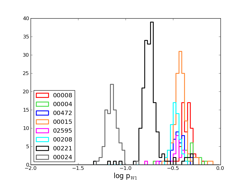
Figure 6: W1 albedo distributions for $8$ asteroid families with more than $20$ measured NIR albedos, identified by the family ID given in Masiero et al. (2013) and Table 2. Families show narrow distributions of albedos correlating with one of three major albedo groupings.

We note that approximately half of the objects fit for the (298) Baptistina family had albedos similar to the Eos family, while the remainder appear to be drawn from the high-albedo group. This result is based on only a small number of measured Baptistina members, and thus is not conclusive, however if confirmed would further impede attempts to assign a unique composition to this family (cf. Reddy et al., 2011) or determine its age and evolution (cf. Masiero et al., 2012b).

Figure 7 shows the proper orbital eccentricity and inclination of all objects with measured $p_{W1}$. The Main Belt is split into three regions by proper semi-major axis ($a$): the inner-Main Belt (IMB, $1.8~{}$AU$<a<2.5~{}$AU), the middle-Main Belt (MMB, $2.5~{}$AU$<a<2.82~{}$AU), and the outer-Main Belt (OMB, $2.82~{}$AU$<a<3.6~{}$AU). We show separately the objects that were associated with an asteroid family by Masiero et al. (2013) and those that are members of the background population. The (221) Eos family stands out distinctly in the belt, although objects with similar $p_{W1}$ are present in the background population in all three regions.

These plots show the clear trend of albedo decreasing with distance from the Sun, however our observational bias against small, low albedo objects amplifies this effect. Broz et al. (2013b), Carruba et al. (2013), and Masiero et al. (2013) observe halos of objects beyond the limits of typical family-identification techniques, however we do not see evidence for these halos in the background population in our dataset. Halos are typically associated with asteroids that have dispersed a large distance from the family center via Yarkovsky and gravitational forces, which will have smaller diameters than objects that were above our sensitivity limit for $p_{W1}$ determination. Our significantly smaller sample size than what is typically used in surveys investigating family halos may also contribute to their absence in our data.

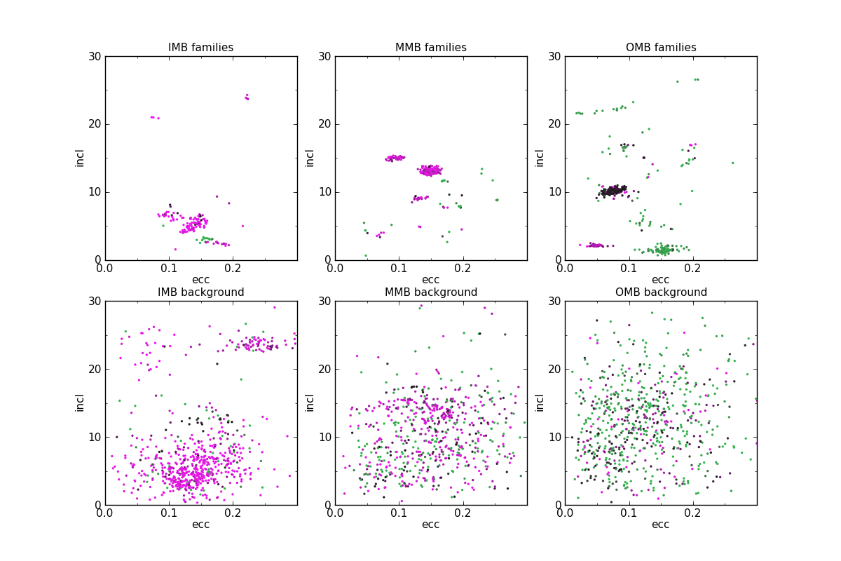
Figure 7: Proper orbital inclination (incl) vs eccentricity (ecc) for inner- (left), middle- (center), and outer-Main Belt populations (right), for objects associated with families (top) and background objects not linked to families (bottom). Colors of the points map the W1 albedo (from green to black to magenta for increasing $p_{W1}$), following Figure 1a.

In Table 2 we present the orbital and physical properties for all families identified in Masiero et al. (2013) that had at least one member with a fitted NIR albedo. We list the name of the family, average proper orbital elements, largest (D_max) and smallest diameter (D_min) represented in our sample, W1 albedos with standard deviations, and number of family members with data sufficient to fit. We also provide for reference the mean $p_{V}$ and standard deviation from Masiero et al. (2013). For cases where only a single body had a measured $p_{W1}$ (often but not always the parent body of the family), D_min is marked with a ‘…’ entry and no standard deviation is given for the mean W1 albedo for families with less than 10 members. Asteroids that have been incorrectly associated with families may have very different mineralogies and thus spectral behavior in the NIR, which could make those objects more likely to fulfill the selection requirements for measured $p_{W1}$. Thus, particular caution is necessary when dealing with families suffering small number statistics, especially families with only a single $p_{W1}$-fit object. We note that the mean $p_{V}$ albedos presented in Masiero et al. (2013) are based on larger numbers of objects and so will generally be more accurate than the mean $p_{W1}$ values given here.

It is also possible to use the W1 albedo to further refine family memberships, particularly for confused cases such as the Nysa-Polana complex. Masiero et al. (2013) divided this complex into a high albedo component with largest body (135) Hertha and a low albedo component with largest body (554) Peraga which is nearly twice the diameter of (142) Polana. We use NIR albedo to reject objects from the low-albedo family that had moderate visible albedos but W1 albedos characteristic of the high-albedo family. Asteroids (261), (1823), (2717), and (15112) can thus be rejected as members of the (554) Peraga group based on W1 albedo. We note that because of a typo in Masiero et al. (2013) (135) Hertha was mistakenly listed as associated with (554) Peraga instead of with its own family, which we correct here. Walsh et al. (2013) present dynamical arguments to divide the (554) Peraga family into two sub-families, however we are unable to see any distinction between these groups in visible or W1 albedo.

Table 2: Average orbital and physical properties for asteroid family members with measured $p_{W1}$. Mean $p_{V}$ values are taken from Masiero et al. (2013)

Family	semimajor axis	eccentricity	inclination	Dmax	Dmin	$<p_{V}>$	$<p_{W1}>$	Sample
	(AU)		(deg)	(km)	(km)			Size
00434	1.937	0.077	20.947	7.62	3.01	0.725 $\pm$ 0.172	0.736	3
00254	2.197	0.122	4.202	11.85	5.71	0.298 $\pm$ 0.105	0.420	7
00008	2.244	0.141	5.251	155.74	3.86	0.291 $\pm$ 0.091	0.435 $\pm$ 0.074	70
00298	2.256	0.148	5.723	12.32	5.36	0.146 $\pm$ 0.034	0.284	9
00163	2.325	0.215	5.008	4.78	…	0.053 $\pm$ 0.016	0.401	1
00587	2.338	0.222	23.901	12.23	4.41	0.310 $\pm$ 0.090	0.421	4
01646	2.353	0.102	8.002	12.47	11.57	0.204 $\pm$ 0.081	0.221	2
00004	2.366	0.101	6.518	109.51	4.53	0.357 $\pm$ 0.110	0.466 $\pm$ 0.129	22
00012	2.390	0.185	8.853	126.64	7.62	0.066 $\pm$ 0.021	0.318	2
00135	2.405	0.178	2.455	82.15	3.77	0.280 $\pm$ 0.088	0.372 $\pm$ 0.071	13
00302	2.407	0.110	1.576	6.11	…	0.062 $\pm$ 0.021	0.422	1
00554	2.418	0.157	3.049	55.18	11.75	0.061 $\pm$ 0.021	0.054 $\pm$ 0.012	13
00752	2.463	0.091	5.049	60.85	…	0.053 $\pm$ 0.014	0.048	1
13698	2.469	0.118	6.534	5.31	…	0.367 $\pm$ 0.098	0.412	1
01658	2.560	0.172	7.749	13.81	5.97	0.255 $\pm$ 0.074	0.343	3
00472	2.562	0.094	15.009	47.04	6.25	0.261 $\pm$ 0.079	0.363 $\pm$ 0.051	39
00005	2.576	0.198	4.514	113.00	…	0.240 $\pm$ 0.105	0.365	1
00606	2.587	0.179	9.631	39.53	…	0.117 $\pm$ 0.028	0.137	1
05079	2.601	0.247	11.730	14.76	…	0.068 $\pm$ 0.020	0.047	1
00404	2.628	0.229	13.062	105.41	73.07	0.060 $\pm$ 0.025	0.059	2
00015	2.630	0.149	13.181	299.21	4.45	0.263 $\pm$ 0.084	0.382 $\pm$ 0.073	126
00569	2.634	0.175	2.659	13.18	…	0.054 $\pm$ 0.016	0.064	1
00145	2.676	0.170	11.642	132.59	14.70	0.062 $\pm$ 0.018	0.055	8
00410	2.727	0.253	8.824	27.28	8.49	0.085 $\pm$ 0.028	0.075	3
00539	2.739	0.164	8.274	56.04	…	0.061 $\pm$ 0.023	0.039	1
00396	2.742	0.168	3.497	37.29	…	0.093 $\pm$ 0.024	0.115	1
00808	2.744	0.132	4.902	37.68	9.51	0.232 $\pm$ 0.071	0.380	2
00363	2.750	0.045	5.480	19.34	…	0.068 $\pm$ 0.018	0.079	1
00128	2.750	0.088	5.181	193.08	…	0.075 $\pm$ 0.024	0.071	1
01734	2.769	0.194	7.951	23.82	8.72	0.056 $\pm$ 0.017	0.074	6
00847	2.777	0.070	3.742	30.08	8.78	0.218 $\pm$ 0.075	0.359	5
00272	2.783	0.048	4.232	25.67	21.09	0.047 $\pm$ 0.014	0.109	3
00322	2.783	0.198	9.521	73.15	…	0.078 $\pm$ 0.027	0.193	1
01128	2.788	0.048	0.659	48.63	…	0.048 $\pm$ 0.013	0.046	1
02595	2.791	0.132	9.068	14.62	6.59	0.262 $\pm$ 0.075	0.343 $\pm$ 0.059	21
01668	2.806	0.178	4.152	25.83	…	0.052 $\pm$ 0.014	0.048	1
03985	2.851	0.123	15.052	22.11	16.19	0.176 $\pm$ 0.058	0.213	3
00081	2.854	0.180	8.233	123.96	…	0.056 $\pm$ 0.016	0.053	1
00208	2.875	0.048	2.129	49.99	10.36	0.237 $\pm$ 0.063	0.335 $\pm$ 0.032	59
00845	2.940	0.036	11.999	58.53	…	0.061 $\pm$ 0.017	0.055	1
00179	2.972	0.076	9.027	74.58	…	0.223 $\pm$ 0.069	0.326	1
00816	3.004	0.145	13.168	50.09	…	0.051 $\pm$ 0.026	0.054	1
00221	3.020	0.077	10.181	95.62	10.03	0.158 $\pm$ 0.048	0.190 $\pm$ 0.065	186
00283	3.070	0.109	8.917	145.55	17.68	0.048 $\pm$ 0.019	0.084	2
02621	3.086	0.128	12.128	47.92	…	0.081 $\pm$ 0.029	0.066	1
01113	3.112	0.137	14.093	48.37	…	0.074 $\pm$ 0.031	0.350	1
00780	3.117	0.070	18.186	114.26	…	0.056 $\pm$ 0.018	0.060	1
01040	3.122	0.197	16.728	22.67	7.56	0.225 $\pm$ 0.075	0.348	4
00511	3.138	0.192	14.439	285.84	23.46	0.065 $\pm$ 0.026	0.076	8
00024	3.142	0.153	1.457	193.54	17.43	0.068 $\pm$ 0.021	0.073 $\pm$ 0.012	95
00928	3.143	0.193	16.359	62.54	24.29	0.075 $\pm$ 0.038	0.057	2
00010	3.143	0.130	5.514	153.58	16.69	0.070 $\pm$ 0.023	0.079 $\pm$ 0.035	17
03330	3.154	0.199	10.149	15.49	…	0.044 $\pm$ 0.015	0.053	1
00490	3.165	0.061	9.323	79.87	…	0.069 $\pm$ 0.022	0.050	1
00778	3.169	0.262	14.282	19.36	…	0.066 $\pm$ 0.020	0.070	1
01306	3.170	0.091	16.448	72.24	15.54	0.061 $\pm$ 0.021	0.107 $\pm$ 0.056	14
00031	3.177	0.196	26.445	281.98	17.31	0.057 $\pm$ 0.016	0.068	3
00618	3.189	0.058	15.879	131.23	…	0.056 $\pm$ 0.018	0.063	1
00702	3.190	0.021	21.598	196.47	26.15	0.066 $\pm$ 0.022	0.071	3
00276	3.190	0.072	22.189	100.36	21.98	0.068 $\pm$ 0.022	0.073 $\pm$ 0.009	11
01303	3.215	0.126	19.023	102.43	28.58	0.049 $\pm$ 0.017	0.069	2
00087	3.485	0.054	9.846	288.38	…	0.057 $\pm$ 0.017	0.082	1

4 Conclusions

We present revised thermal model fits for Main Belt asteroids, allowing for the albedo in each of the near-infrared reflected wavelengths to be fit independently. The $3.4~{}\mu$m and $4.6~{}\mu$m spectral regions covered by the WISE/NEOWISE W1 and W2 bandpasses are poorly probed in ground-based spectroscopy but can be used to provide insight into asteroid mineralogical composition by constraining spectral slope. In total we present $3080$ fits of $p_{W1}$ and/or $p_{W2}$ for $2835$ unique Main Belt objects.

The MBA population has three distinct peaks in our observed $p_{W1}$ distribution at $p_{W1}\sim 0.06$, $p_{W1}\sim 0.16$, and $p_{W1}\sim 0.4$. The high and low $p_{W1}$ peaks correspond to the high and low visible albedo groups observed previously, while the moderate $p_{W1}$ peak corresponds to an intermediate visible albedo that is blended with the high $p_{V}$ objects in visible albedo distributions. The distribution of albedos we measure have a larger fraction of high-albedo objects than what was observed for the MBA visible albedo distribution, however this is an effect of the biases in our sample selection.

Asteroid families have narrow $p_{W1}$ distributions corresponding to one of the three observed $p_{W1}$ peaks. The (221) Eos family represents the only significant concentration of objects near the peak at $p_{W1}\sim 0.16$, although other objects with this albedo that are not related to asteroid families are scattered throughout the entire Main Belt region. This family also corresponds to an unusual ‘end member’ taxonomic classification, K-type, that has been suggested to correspond to a partially differentiated parent or olivine-rich mineralogy. NIR albedo measurements provide a way to rapidly search the known population for candidate K-type objects in the Main Belt, and are a powerful tool that acts as a proxy for asteroid taxonomic type.

Our results show that the majority of high albedo objects, believed to have surface compositions dominated by silicates and similar to ordinary chondrite meteorites, show an overall reddening from visible to W1 wavelengths similar to what is seen in the NIR. The spectra become blue from W1 to W2, which is also seen in some meteorite populations, particularly the Eucrites. This overall picture is consistent with a primarily-silicate dominated composition. Objects with moderate infrared albedos show similar behavior across the wavelengths probed here, although the lower albedo value at W1 may indicate subtle differences in composition from the high albedo population or even a mix of different mineralogies.

The low albedo objects in our sample show a much wider range of behavior in these spectral regions. Many object show red slopes across all wavelengths consistent with the NIR spectral behavior of C/D/P-type objects. However approximately $10\%$ of our population show a blue slope from visible to W1, even in spite of the biases against blue-sloped, low-albedo objects in our sample. These objects are associated with B and Ch spectral taxonomies. The blue visible-to-W1 spectral slope in the Ch class objects may be indicative of a significant absorption feature at W1 wavelengths from minerals such as carbonates.

The fits presented here are based on reflected light, and thus our sample will not accurately represent the true distribution of $p_{W1}$ or $p_{W2}$. Small, low albedo asteroids as well as objects with blue NIR spectral slopes are more likely to be undetected in the W1 and/or W2 wavelengths and thus underrepresented in our population distributions. A larger survey with greater sensitivity in these spectral regions is required to extend these results to a population comparable to the one with measured diameters and visible albedos.

References

- Bowell et al. (1989) Bowell, E., Hapke, B., Domingue, D., Lumme, K., Peltoniemi, J. & Harris, A.W., 1989, Asteroids II, University of Arizona Press, 524.
- Broz & Morbidelli (2013a) Broz, M. & Morbidelli, A., 2013a, Icarus, 223, 844
- Broz et al. (2013b) Broz, M., Morbidelli, A., Bottke, W.F., Rozehnal, J., Vokrouhlický & D., Nesvorný, D., 2013b, A&A, 551, A117
- Campins et al. (2010) Campins, H., Hargrove, K., Pinilla-Alonso, N., Howell, E.S., et al., 2010, Nature, 464, 1320.
- Carruba et al. (2013) Carruba, V., Domingos, R.C., Nesvorny, D., Roig, F., Huaman, M.E., Souami, D., 2013, MNRAS, 433, 2075.
- Clark et al. (2009) Clark, B.E., Ockert-Bell, M.E., Cloutis, E.A., et al., 2009, Icarus, 202, 119.
- Cutri et al. (2012) Cutri, R.M., Wright, E.L., Conrow, T., Bauer, J., et al., 2012, “Explanatory Supplement to the WISE All-Sky Data Release Products”, http://wise2.ipac.caltech.edu/docs/release/allsky/expsup/index.html.
- DeMeo et al. (2009) DeMeo, F.E., Binzel, R.P., Slivan, S.M. & Bus, S.J., 2009, Icarus, 202, 160.
- DeMeo & Carry (2013) DeMeo, F.E. & Carry, B., 2013, Icarus, 226, 723.
- DeMeo et al. (2014) DeMeo, F.E., Binzel, R.P., Carry, B., Polishook, D., & Moskovitz, N.A, 2014, Icarus, 229, 392
- Gaffey et al. (2002) Gaffey, M.J., Cloutis, E.A., Kelley, M.S. & Reed, K.L., 2002, Asteroids III, W. F. Bottke Jr., A. Cellino, P. Paolicchi, and R. P. Binzel (eds), University of Arizona Press, 183.
- Grav et al. (2011a) Grav, T., Mainzer, A., Bauer, J., et al., 2011a, ApJ, 742, 40.
- Grav et al. (2011b) Grav, T., Mainzer, A., Bauer, J., et al., 2011b, ApJ, 744, 197.
- Grav et al. (2012) Grav, T., Mainzer, A.K., Bauer, J.M., Masiero, J.R., Nugent, C.R., 2012, ApJ, 759, 49.
- Hardersen et al. (2011) Hardersen, P.S, Cloutis, E.A., Reddy, V., et al., 2011, M&PS, 46, 1910.
- Harris (1998) Harris, A.W., 1998, Icarus, 131, 291.
- Harris & Drube (2014) Harris, A.W. & Drube, L., 2014, ApJL, 785, 4
- Levison et al. (2009) Levison, H.F., Bottke, W.F., Gounelle, M., et al., 2009, Nature, 460, 364.
- Mainzer et al. (2011a) Mainzer, A.K., Bauer, J.M., Grav, T., Masiero, J., Cutri, R.M., Dailey, J., Eisenhardt, P., McMillan, R.M. et al., 2011a, ApJ, 731, 53.
- Mainzer et al. (2011b) Mainzer, A.K., Grav, T., Masiero, J., Bauer, J.M., Wright, E., Cutri, R.M., McMillan, R.S., Cohen, M., Ressler, M., Eisenhardt, P., 2011b, ApJ, 736, 100.
- Mainzer et al. (2011c) Mainzer, A.K., Grav, T., Masiero, J., Bauer, J.M., Wright, E., Cutri, R.M., Walker, R. & McMillan, R.S., 2011c, ApJL, 737, 9.
- Mainzer et al. (2011d) Mainzer, A.K., Grav, T., Masiero, J., et al., 2011d, ApJ, 741, 90.
- Mainzer et al. (2011e) Mainzer, A., Grav, T., Bauer, J.M., Masiero, J., et al., 2011e, ApJ, 743, 156.
- Mainzer et al. (2012) Mainzer, A.K., Grav, T., Masiero, J., Bauer, J.M., Cutri, R.M., McMillan, R.S., Nugent, C., Tholen, D., Walker, R. & Wright, E.L., 2012, ApJL, 760, 12.
- Mainzer et al. (2014) Mainzer, A.K., Bauer, J.M., Grav, T., Masiero, J., et al., 2014, ApJ, submitted.
- Masiero et al. (2011) Masiero, J.R., Mainzer, A.K., Grav, T., Bauer, J.M., Cutri, R.M., Dailey, J., Eisenhardt, P.R.M, et al., 2011, ApJ, 741, 68.
- Masiero et al. (2012a) Masiero, J.R., Mainzer, A.K., Grav, T., Bauer, J.M., Cutri, R., Nugent, C. & Cabrera, M.S., 2012, ApJ, 759, L8.
- Masiero et al. (2012b) Masiero, J.R., Mainzer, A.K., Grav, T., Bauer, J.M. & Jedicke, R., 2012, ApJ, 759, 14.
- Masiero et al. (2013) Masiero, J.R., Mainzer, A.K., Bauer, J.M., Grav, T., Nugent, C., Stevenson, R., 2013, ApJ, 770, 7.
- Menke (2005) Menke, J., 2005, Minor Planet Bulletin, 32, 85.
- Morbidelli et al. (2005) Morbidelli, A., Levison, H.F., Tsiganis, K. & Gomes, R., 2005, Nature, 435, 462.
- Mothé-Diniz (2005) Mothé-Diniz, T. & Carvano, J.M., 2005, A&A, 442, 727.
- Neese (2010) Neese, C., Ed., Asteroid Taxonomy V6.0. EAR-A-5-DDR-TAXONOMY-V6.0. NASA Planetary Data System, 2010.
- Reddy et al. (2011) Reddy, V., Carvano, J.M., Lazzaro, D., et al., 2011, Icarus, 216, 184.
- Reddy et al. (2012a) Reddy, V., Nathues, A., Le Corre, L., et al., 2012a, Science, 336, 700.
- Reddy et al. (2012b) Reddy, V., Sanchez, J., Nathues, A., et al., 2012b, Icarus, 217, 153.
- Rivkin & Emery (2010) Rivkin, A.S. & Emery, J.P., 2010, Nature, 464, 1322.
- Walsh et al. (2013) Walsh, K.J., Delbó, M., Bottke, W.F., Vokrouhlický, D. & Lauretta, D.S., 2013, Icarus, 225, 283.
- Wright et al. (2010) Wright, E.L., Eisenhardt, P., Mainzer, A.K., Ressler, M.E., Cutri, R.M., Jarrett, T., Kirkpatrick, J.D., Padgett, D., et al., 2010, AJ, 140, 1868.