New insight into $nd\rightarrow$ ${}^{3}H\gamma$ process at thermal energy with pionless effective field theory

Abstract

We take a new look at the neutron radiative capture by a deuteron at thermal energy with the pionless effective field theory (EFT($\pi\!\!\!/$)) approach. We present in detail the calculation of $nd\rightarrow$ ${}^{3}H\gamma$ amplitudes for incoming doublet and quartet channels leading to the formation of a triton fully in the projection method based on the cluster-configuration space approach. In the present work, we consider all possible one-body and two-body photon interaction diagrams. In fact, additional diagrams that make significant changes in the results of the calculation of the total cross section in the $nd\rightarrow$ ${}^{3}H\gamma$ process are included in this study. The properly normalized triton wave function is calculated and taken into consideration. We compare the cross section of the dominant magnetic M1-transition of $nd\rightarrow$ ${}^{3}H\gamma$ up to next-to-next-to-leading order $\textrm{N}^{2}\textrm{LO}$ with the results of the previous model-dependent theoretical calculations and experimental data. The more acceptable results for cross section $\sigma^{(2)}_{tot}=0.297\;(\textrm{LO})+0.124\;(\textrm{NLO})+0.048\;(\textrm{N}^{2}\textrm{LO})=[0.469\pm 0.033]\>\textrm{mb}$ show order by order convergence and cutoff independence. No three-body currents are needed to renormalize observables up to $\textrm{N}^{2}\textrm{LO}$ in this process.

I Introduction

Studies of the radiative capture reactions on numerous light atomic nuclei have been continued at thermal and astrophysical energies with the model-independent pionless effective field theory (EFT($\pi\!\!\!/$)) approach in the recent years Rupak-np -Acharya-phillips .

The calculation of radiative capture amplitude and cross section of $nd\rightarrow$ ${}^{3}H\gamma$ and $pd\rightarrow$ ${}^{3}H\!e\,\gamma$ are an essential input in the calculation of the parity-violating radiative capture of the above processes at the thermal energy Moskalev ; desplanques-benayoun ; moeini-bayegan .

In the present paper, we study the $nd\rightarrow$ ${}^{3}H\gamma$ process fully with the projection operator method based on the cluster-configuration space which is introduced by 20 of sadeghi-bayegan . We also consider the calculation of observables with M1 transition up to next-to-next-to-leading order ($\textrm{N}^{2}\textrm{LO}$) with the following significant changes in comparison with the previous EFT($\pi\!\!\!/$) calculation sadeghi-bayegan-grieshammer : a) including the diagrams with radiation from external nucleon leg, external deuteron leg, and on-shell two-body bubble (see the diagrams ”$a_{0}$”, ”$a_{1}$”, and ”$a_{3}$” in Fig.1 of page 1), b) considering both contributions corresponding to two nucleon poles before and after photon creation in the first diagram of the second row in Fig.1, c) inserting the diagram with the radiation directly from the exchanged nucleon, d) adding the contribution of the ${}^{3}S_{1}\rightarrow^{3}S_{1}$ M1 transition and e) introducing .and using the properly normalized triton wave function.

The triton or helium-three wave functions consist of two parts, one is the nucleon and dibaryon cluster wave function and the other is the two nucleon structure of the dibaryon cluster. We follow the Bethe-Salpeter (BS) equation in adam ; book for normalization and we use the normalization condition of the relativistic two-body vertex function and work out the nonrelativistic one which is suitable for neutron-deuteron ($nd$) scattering leading to the formation of a triton.

The theoretical calculations of the observables in the $nd\rightarrow$ ${}^{3}H\gamma$ process were previously performed based on model-dependent approaches Faldt et al . The cross section and polarization observables were studied theoretically for radiative capture reactions ${}^{2}H$$(n,\gamma)$${}^{3}H$ and ${}^{2}H$$(p,\gamma)$${}^{3}He$ at low energies viviani et al . The cross section for thermal neutron radiative capture on the deuteron was measured to be $\sigma_{tot}^{exp}=0.508\pm 0.015$ mb Jurney et al , in agreement with the results of earlier experiments Kaplan et al ; Merritt et al .

In the present work, the calculation of all M1 diagrams are calculated for the incoming doublet and quartet $nd$ channels fully in the cluster-configuration space up to $\textrm{N}^{2}\textrm{LO}$ in Sec.II. The calculation of the cross section for $nd\rightarrow$ ${}^{3}H\gamma$ is presented in Sec.III. In Sec.IV numerical aspects of the calculation of M1 amplitudes are discussed. The results and comparison with other theoretical and experimental works are explained in Sec.V. Finally, we summarize the paper and discuss future investigations in Sec.VI.

II $nd\rightarrow$ ${}^{3}H\gamma$ system

In this section, we focus on the introduction of the EFT($\pi\!\!\!/$) amplitude for the $nd\rightarrow$ ${}^{3}H\gamma$ process up to $\textrm{N}^{2}\textrm{LO}$. We concentrate on the zero-energy regime and try to calculate the amplitude of the neutron radiative capture by deuteron at thermal energy ($2.5\times 10^{-8}$ MeV) in the center-of-mass (c.m.) frame.

In the EFT($\pi\!\!\!/$) method, the electromagnetic (EM) interactions in the three-body systems can be inserted principally by considering the one-, two-, and three-body currents. However, we show that the cutoff independence is achieved up to $\textrm{N}^{2}\textrm{LO}$ with one- and two-body currents and therefore there is no need for additional three-body currents up to $\textrm{N}^{2}\textrm{LO}$ calculations. In the very-low-energy regime the M1 transition has a dominant piece in the amplitude of $nd\rightarrow$ ${}^{3}H\gamma$. E2 transition also contribute to the $nd\rightarrow$ ${}^{3}H\gamma$ reaction but comparing with the M1 interaction, it has a negligible contribution. In the following, we evaluate the EFT($\pi\!\!\!/$) amplitude of the neutron radiative capture by deuteron reaction by considering the dominant M1 transitions using one- and two-body currents up to $\textrm{N}^{2}\textrm{LO}$.

Note that the convection current of the proton (E1 transition) has odd parity (due to one power of nucleon momentum), so this mixes an incoming P-wave state to the final S-wave triton. Capture from the P wave introduces the factor of the external nucleon momentum forcing the amplitude to vanish at threshold.

The Lagrangian of the S-wave strong interactions using a dibaryon auxiliary field are given by phillips-rupak-savage ; 20 of sadeghi-bayegan

$$\mathcal{L}_{S}=N^{\dagger}\Big{(}iD_{0}+\frac{\vec{D}^{2}}{2m_{N}}\Big{)}N+d^{A^{\dagger}}_{s}\Big{[}\Delta_{s}-c_{0s}\Big{(}iD_{0}+\frac{\vec{D}^{2}}{4m_{N}}+\frac{\gamma^{2}_{s}}{m_{N}}\Big{)}\Big{]}d^{A}_{s}\qquad\qquad\qquad\qquad\quad$$

$$+d^{i^{\dagger}}_{t}\Big{[}\Delta_{t}-c_{0t}\Big{(}iD_{0}+\frac{\vec{D}^{2}}{4m_{N}}+\frac{\gamma^{2}_{t}}{m_{N}}\Big{)}\Big{]}d^{i}_{t}-y\Big{(}d^{A^{\dagger}}_{s}(N^{\dagger}P^{A}N)+d^{i^{\dagger}}_{t}(N^{\dagger}P^{i}N)+h.c.\Big{)}\quad\!\!\!$$

$$+\frac{m_{N}y^{2}\mathcal{H}(E,\Lambda)}{6}\;N^{\dagger}\bigg{(}\big{(}d^{i}_{t}\sigma_{i}\big{)}^{\dagger}\big{(}d^{j}_{t}\sigma_{j}\big{)}-\big{[}\big{(}d^{i}_{t}\sigma_{i}\big{)}^{\dagger}\big{(}d^{A}_{s}\sigma_{A}\big{)}+h.c.\big{]}+\big{(}d^{A}_{s}\tau_{A}\big{)}^{\dagger}\big{(}d^{B}_{s}\sigma_{B}\big{)}\bigg{)}N\!\!\!\!\!\!\!\!$$

$$+\cdot\cdot\cdot\,,\;\quad\qquad\qquad\qquad\qquad\qquad\qquad\qquad\qquad\qquad\qquad\qquad\qquad\qquad\qquad\qquad\>\;$$ (1)

where $D_{\mu}$ is the covariant derivative which acts on the nucleon and dibaryon fields with $\partial_{\mu}+ie\frac{1+\tau_{3}}{2}A_{\mu}$ and $\partial_{\mu}+ieCA_{\mu}$ relations, respectively. $A_{\mu}$ is the external field and $C=2,1,$ and $0$ for proton-proton, neutron-neutron and neutron-neutron dibaryons. The center dots in the last line denotes the other suppressed terms. In Eq.(II), $N$ is the nucleon iso-doublet field. The dibaryon auxiliary fields for deuteron and iso di-nucleon systems are introduced by $d^{i}_{t}$ and $d^{A}_{s}$, respectively. The operators $P^{i}=\frac{1}{\sqrt{8}}\sigma_{2}\sigma^{i}\tau_{2}$ and $P^{A}=\frac{1}{\sqrt{8}}\sigma_{2}\tau_{2}\tau^{A}$ with $\tau_{A}$ ($\sigma_{i}$) as isospin (spin) Pauli matrices are the projection operators of nucleon-nucleon ($NN$) ${}^{3}S_{1}$ and ${}^{1}S_{0}$ states, respectively. $m_{N}$ represents the nucleon mass and the three-nucleon force is introduced by $\mathcal{H}(E,\Lambda)$, where $E$ and $\Lambda$ are the total energy and cutoff momentum. The $\mathcal{H}(E,\Lambda)$, which absorbs all dependence on the cutoff as $\Lambda\rightarrow\infty$, is given by Bedaque-H-vK ; Bedaque-H-vK-2 ; Bedaque-R-H

$$\mathcal{H}(E,\Lambda)=\frac{2}{\Lambda^{2}}\sum_{m=0}^{\infty}H_{2m}(\Lambda)\bigg{(}\frac{m_{N}E+\gamma_{t}^{2}}{\Lambda^{2}}\bigg{)}^{m}=\frac{2H_{0}(\Lambda)}{\Lambda^{2}}+\frac{2H_{2}(\Lambda)}{\Lambda^{4}}(m_{N}E+\gamma_{t}^{2})+\cdot\cdot\cdot\,,$$ (2)

where the interactions proportional to $H_{2m}$ enter at $\textrm{N}^{2m}\textrm{LO}$ Bedaque-R-H .

In our calculation, we consider generally $y^{2}=\frac{4\pi}{m_{N}}$. The parameters $\Delta_{s/t}$ and $c_{0s/t}$ are given by matching the EFT($\pi\!\!\!/$) $NN$ scattering amplitude to the effective range expansion (ERE) of the scattering amplitude of two non-relativistic nucleons around the $i\gamma_{s/t}$ 20 of sadeghi-bayegan . $\gamma_{t}=45.7025$ MeV is the binding momentum of the deuteron and $\gamma_{s}=\frac{1}{a_{s}}$ with $a_{s}=-23.714$ fm as the scattering length in the ${}^{1}S_{0}$ state.

The Lagrangian of the M1 interaction is constructed by considering the nucleon and dibaryon operators coupling to the magnetic field $\vec{B}$,

$$\mathcal{L}_{B}=\frac{e}{2m_{N}}N^{\dagger}\big{(}k_{0}+k_{1}\tau^{3}\big{)}\vec{\sigma}\cdot\vec{B}N+e\frac{L_{1}}{m_{N}\sqrt{\rho_{d}r_{0}}}d^{j^{\dagger}}_{t}d^{3}_{s}B_{j}-e\frac{2L_{2}}{m_{N}\rho_{d}}i\,\epsilon_{ijk}\,d^{i^{\dagger}}_{t}d^{j}_{t}B_{k}+h.c.\,.$$ (3)

In the above equation, $k_{0}=\frac{1}{2}(k_{p}+k_{n})=0.4399$ and $k_{1}=\frac{1}{2}(k_{p}-k_{n})=2.35294$ with $k_{p}$ ($k_{n}$) as the proton (neutron) magnetic moment are the isoscalar and isovector nucleon magnetic moments, respectively. $e$ is the electric charge and $\rho_{d}=1.764$ fm ($r_{0}=2.73$ fm) denotes the effective range of the triplet (singlet) $NN$ state. The coefficients $L_{1}=-4.427\pm 0.015$ fm and $L_{2}=-0.4$ fm, which enter at next-to-leading order (NLO), have been fixed from the cross section of $np\rightarrow$ $d\gamma$ at thermal energy, $\sigma^{exp}_{np\rightarrow\,d\gamma}=334.2\pm 0.5$ mb and the deuteron magnetic moment $\mu_{M}$, respectively Ando-Hyun .

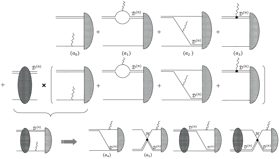
Figure 1: The M1 $nd\rightarrow$ ${}^{3}H\gamma$ diagrams at $\textrm{N}^{n}\textrm{LO}$ ($n\leq 2$). The ”⁽ⁿ⁾” superscript denotes the contribution up to $\textrm{N}^{n}\textrm{LO}$. All possible diagrams in the M1 transition of the $nd\rightarrow$ ${}^{3}H\gamma$ process up to $\textrm{N}^{n}\textrm{LO}$ are shown in the first and second lines. The diagrams in the third line are the expanded version of the first diagram in the second line. The solid, wavy, and double lines represent a nucleon, a photon, and a dibaryon field, respectively. The nucleon-nucleon-photon ($NN\gamma$) and dibaryon-dibaryon-photon ($dd\gamma$) vertices show the one- and two-body M1 interactions. $\mathcal{D}^{(n)}$ is the $2\times 2$ propagator matrix of the dibaryon auxiliary fields and the three-body force is indicated by $\mathcal{H}$. The dashed oval and dashed half oval denote the $Nd$ scattering amplitude and the normalized triton wave function up to $\textrm{N}^{n}\textrm{LO}$, respectively.

The diagrams of the M1 transition in the $nd\rightarrow$ ${}^{3}H\gamma$ process up to $\textrm{N}^{n}\textrm{LO}$ ($n\leq 2$) are schematically shown in Fig.1. Note that in the entire paper, the superscript ”(n)” denotes the contribution from the sum of all pieces up to, and including, order n. $\mathcal{D}^{(n)}$ indicates the propagator of the dibaryon fields up to $\textrm{N}^{n}\textrm{LO}$ which is given in the cluster-configuration space as

$$\mathcal{D}^{(n)}(q_{0},q)=\left(\begin{array}[]{cc}D_{t}^{(n)}(q_{0}-\frac{q^{2}}{2m_{N}},q)&0\\ 0&D_{s}^{(n)}(q_{0}-\frac{q^{2}}{2m_{N}},q)\\ \end{array}\right),$$ (6)

where

$$D^{(n)}_{t}(q_{0},q)=\frac{1}{\gamma_{t}-\sqrt{\frac{q^{2}}{4}-m_{N}q_{0}-i\varepsilon}}\sum^{n}_{m=0}\bigg{(}\frac{\frac{\rho_{d}}{2}(m_{N}q_{0}-\frac{q^{2}}{4}+\gamma_{t}^{2})}{\gamma_{t}-\sqrt{\frac{q^{2}}{4}-m_{N}q_{0}-i\varepsilon}}\bigg{)}^{m},$$

$$D^{(n)}_{s}(q_{0},q)=\frac{1}{\gamma_{s}-\sqrt{\frac{q^{2}}{4}-m_{N}q_{0}-i\varepsilon}}\sum^{n}_{m=0}\bigg{(}\frac{\frac{r_{0}}{2}(m_{N}q_{0}-\frac{q^{2}}{4})}{\gamma_{s}-\sqrt{\frac{q^{2}}{4}-m_{N}q_{0}-i\varepsilon}}\bigg{)}^{m}.$$ (7)

We emphasize that the above propagators can be applied up to $\textrm{N}^{3}\textrm{LO}$ and should be corrected for the higher orders.

In Fig.1, the dashed oval denotes the nucleon-deuteron ($Nd$) scattering amplitudes which are presented by $t^{(n)}_{d}$ and $t^{(n)}_{q}$ for the doublet and quartet channels up to $\textrm{N}^{n}\textrm{LO}$, respectively. The Faddeev equations of $t^{(n)}_{d/q}$ are introduced in Appendix A. The dashed half oval indicates the normalized triton wave function up to $\textrm{N}^{n}\textrm{LO}$ which is introduced by $t^{(n)}_{{}^{3}H}$ in the following. The procedure of making the triton wave function and its normalization condition are briefly presented in Appendix B.

We consider the contribution of all diagrams shown in Fig.1 in the amplitude of neutron radiative capture by a deuteron reaction. The third diagram of the second line and all diagrams of the first line in Fig.1 have not been considered in the previous EFT($\pi\!\!\!/$) calculations of the $nd\rightarrow$ ${}^{3}H\gamma$ amplitude sadeghi-bayegan ; sadeghi-bayegan-grieshammer . We have also added the contribution of the ${}^{3}S_{1}\rightarrow^{3}$$S_{1}$ M1 transition to the amplitude of the $nd\rightarrow$ ${}^{3}H\gamma$ process which was previously not considered in sadeghi-bayegan ; sadeghi-bayegan-grieshammer . This two-body M1 transition is indicated in the Lagrangian of Eq.(3) by the $L_{2}$ coefficient which enters first at NLO as $L_{1}$. However the contribution of the ${}^{3}S_{1}\rightarrow^{3}$$S_{1}$ M1 transition is small at NLO but its effect is significant at $\textrm{N}^{2}\textrm{LO}$.

Before we evaluate the contribution of the diagrams in Fig.1, let us make a comment about the computational process of the amplitude at NLO and $\textrm{N}^{2}\textrm{LO}$. Introducing the $\textrm{N}^{n}\textrm{LO}$ diagrams as in Fig.1, includes some diagrams of higher order, for example the NLO calculation includes $\textrm{N}^{2}\textrm{LO}$, $\textrm{N}^{3}\textrm{LO}$ and $\textrm{N}^{4}\textrm{LO}$ terms. So, this calculation includes higher-order terms, but it is not - or at least, not immediately - a full higher-order correction, and so does not achieve that precision. On the other hand, the additional diagrams are small in a well behaved expansion, so the precision is not compromised. This procedure is made only for convenience in the computational process.

Now, we make a comment about the evaluation of the first diagram in the second line of Fig.1. This diagram is different somewhat from other ones because it has two contributions corresponding to the poles in the nucleon propagators before and after the photon creation. Therefore, these two poles are corresponding to two contributions, one is that the photon is emitted during the exchange of a nucleon and the other is that the photon is emitted after exchanging the nucleon. If we add the half-offshell $Nd$ scattering amplitude from left to the first diagram in the first line of Fig.1, we miss the contribution of the case that the photon emission occurs during the nucleon exchange. So, we have to replace the half-offshell $Nd$ scattering amplitude by four diagrams which are introduced in Fig.4. Thus, we must substitute the first diagrams of the second line by four diagrams introduced in the third line of Fig.1. The effect of the photon emitted during the exchange of another nucleon can also be applied when the triton formation precedes the photon-nucleon interaction. But the evaluation of this effect makes no significant changes in the final results.

By working in the Coulomb gauge, the M1 amplitude of the $nd\rightarrow$ ${}^{3}H\gamma$ can be written as two orthogonal terms,

$$\big{(}t^{\dagger}\sigma_{a}N\big{)}\big{(}\vec{\varepsilon}_{d}\times\big{(}\vec{\varepsilon}^{\ast}_{\gamma}\times\vec{\tilde{q}}\big{)}\big{)}_{a}\>,\qquad i\big{(}t^{\dagger}N\big{)}\big{(}\vec{\varepsilon}_{d}\cdot\vec{\varepsilon}^{\ast}_{\gamma}\times\vec{\tilde{q}}\big{)}\,,\;\;\;$$ (8)

with $t$, $\vec{\varepsilon}_{\gamma}$, $\vec{\varepsilon}_{d}$, and $\vec{\tilde{q}}$ are the final ${}^{3}H$ (or ${}^{3}He$) field, the three-vector polarization of the produced photon, the three-vector polarization of the deuteron and the unit vector along the 3-momentum of the photons, respectively.

In the $nd\rightarrow$ ${}^{3}H\gamma$ process, two initial doublet (${}^{2}S_{\frac{1}{2}}$) and quartet (${}^{4}S_{\frac{3}{2}}$) channels can make the final triton state using the M1 transition. If we evaluate the contributions of all diagrams in Fig.1, we can generally write the $\textrm{N}^{n}\textrm{LO}$ ($n\leq 2$) amplitude of the $nd\rightarrow$ ${}^{3}H\gamma$ process as

$$\mathcal{W}^{(n)}=t^{\dagger}\big{[}\mathcal{M}^{(n)}_{d}Y_{d}+\mathcal{M}^{(n)}_{q}Y_{q}]N$$ (9)

where

$$Y_{d}=i\vec{\varepsilon}_{d}\cdot\vec{\varepsilon}^{\ast}_{\gamma}\times\vec{\tilde{q}}+\vec{\sigma}\times\vec{\varepsilon}_{d}\cdot\vec{\varepsilon}^{\ast}_{\gamma}\times\vec{\tilde{q}}\,,\>\,$$

$$Y_{q}=2\,i\vec{\varepsilon}_{d}\cdot\vec{\varepsilon}^{\ast}_{\gamma}\times\vec{\tilde{q}}-\vec{\sigma}\times\vec{\varepsilon}_{d}\cdot\vec{\varepsilon}^{\ast}_{\gamma}\times\vec{\tilde{q}}\,.$$ (10)

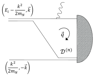
Figure 2: The $a_{4}$ diagram in Fig.1. $k$ and $E_{i}$ denote the incoming c.m. momentum and the total energy of the initial $nd$ system, respectively. All notation are the same as in Fig.1.

For example, we concentrate on the detailed evaluation of the diagram $a_{4}$ contribution. The energy and momentum of the incoming particles are shown in Fig.2. We start by writing the amplitude of the diagram in Fig.2 using the Lagrangians in Eqs.(II) and (3). Generally, before applying the projection operators, we can write the contribution of the diagrams in Fig.2 in the cluster-configuration space up to $\textrm{N}^{n}\textrm{LO}$ ($n\leq 2$) as

$$\bar{S}^{(n)}_{4,unproj.}(E_{i},k)=i\frac{e\,y^{2}}{16m_{N}}\,\int\frac{d^{4}q}{(2\pi)^{4}}\,t^{(n)^{\dagger}}_{{}^{3}\!H}(q)\frac{1}{q_{0}-E_{i}+E_{f}-\frac{q^{2}}{2m_{N}}+i\varepsilon}\qquad$$

$$\times\frac{1}{q_{0}-\frac{q^{2}}{2m_{N}}+i\varepsilon}\,\frac{1}{E_{i}-q_{0}-\frac{k^{2}}{2m_{N}}-\frac{(\vec{k}+\vec{q})^{2}}{2m_{N}}+i\varepsilon}\mathcal{D}^{(n)}(E_{i},q)$$

$$\times\left(\begin{array}[]{cc}(k_{0}+k_{1}\tau_{3})\sigma_{k}\sigma_{s}\sigma_{r}B_{k}&(k_{0}+k_{1}\tau_{3})\sigma_{k}\tau_{A}\sigma_{r}B_{k}\\ (k_{0}+k_{1}\tau_{3})\sigma_{k}\sigma_{s}\tau_{B}B_{k}&(k_{0}+k_{1}\tau_{3})\sigma_{k}\tau_{A}\tau_{B}B_{k}\\ \end{array}\right),\qquad\!\!$$ (13)

where $k$ is the incoming momentum and $E_{i}=\frac{3k^{2}}{4m_{N}}-\frac{\gamma_{t}^{2}}{m_{N}}$ denotes the energy of the initial $nd$ system. $E_{f}$ represents the final state energy which is given by $E_{f}=-B_{t}$ with $B_{t}=8.48$ MeV as the binding energy of the triton. The $s$ ($A$) and $r$ ($B$) indices are the spin (isospin) components of the incoming and outgoing dibaryons. To solve the energy integration, we introduce the poles of Eq.(II) in the complex plane. It is obvious that we have the three following pole:

$$q_{0}=\frac{q^{2}}{2m_{N}}-i\varepsilon,\qquad\qquad\qquad\quad$$

$$q_{0}=E_{i}-E_{f}+\frac{q^{2}}{2m_{N}}-i\varepsilon,\qquad\;$$

$$q_{0}=E_{i}-\frac{k^{2}}{2m_{N}}-\frac{(\vec{k}+\vec{q})^{2}}{2m_{N}}+i\varepsilon,$$ (14)

where they result from the denominator of the nucleon propagators. With respect to the poles in Eq.(II) and doing the integration over energy and the solid angle, the $\bar{S}^{(n)}_{4,unproj.}(E_{i},k)$ is

$$\bar{S}^{(n)}_{4,unproj.}(E_{i},k)=\frac{e\,y^{2}}{32\pi^{2}}\frac{1}{E_{f}-E_{i}}\,\int^{\Lambda}_{0}dq\,q^{2}\,t^{(n)^{\dagger}}_{{}^{3}\!H}(q)\qquad\qquad\qquad\qquad\qquad\qquad\qquad\qquad$$

$$\times\frac{1}{kq}\bigg{[}\mathcal{D}^{(n)}(E_{i},q)Q_{0}(\frac{m_{N}E_{i}-k^{2}-q^{2}}{kq})-\mathcal{D}^{(n)}(E_{f},q)Q_{0}(\frac{m_{N}E_{f}-k^{2}-q^{2}}{kq})\bigg{]}$$

$$\times\left(\begin{array}[]{cc}(k_{0}+k_{1}\tau_{3})\sigma_{k}\sigma_{s}\sigma_{r}B_{k}&(k_{0}+k_{1}\tau_{3})\sigma_{k}\tau_{A}\sigma_{r}B_{k}\\ (k_{0}+k_{1}\tau_{3})\sigma_{k}\sigma_{s}\tau_{B}B_{k}&(k_{0}+k_{1}\tau_{3})\sigma_{k}\tau_{A}\tau_{B}B_{k}\\ \end{array}\right).\qquad\qquad\qquad\qquad\qquad$$ (17)

with $Q_{0}(z)$ as the zeroth Legendre polynomial of the second kind. In order to obtain the contribution of the diagram in Fig.2 for the $nd\rightarrow$ ${}^{3}H\gamma$ reaction, we have to project the initial $Nd$ system to the doublet and quartet cases (corresponding to two possible M1 transitions) while the final state should be ${}^{2}S_{\frac{1}{2}}$ because of the triton. The contribution of the M1 transition with the initial quartet channel (${}^{4}S_{\frac{3}{2}}$) is calculated by applying the projection operators

$$\mathcal{P}_{d,rB}=\frac{1}{\sqrt{3}}\left(\begin{array}[]{cc}\sigma_{r}&0\\ 0&\tau_{B}\\ \end{array}\right),$$ (20)

and

$$\mathcal{P}^{s}_{q,l}=\left(\begin{array}[]{cc}\delta^{s}_{l}-\frac{1}{3}\sigma^{s}\sigma_{l}&0\\ 0&0\\ \end{array}\right),$$ (23)

with $l$ as the spin component of the deuteron in the quartet channel, from left and right in Eq.(II), respectively. So, we gain

$$\bar{S}^{(n)}_{4,q}(E_{i},k)=\frac{e\,y^{2}}{24\sqrt{3}\pi^{2}}\frac{1}{E_{f}-E_{i}}\,\int^{\Lambda}_{0}dq\,q^{2}\,t^{(n)^{\dagger}}_{{}^{3}\!H}(q)\qquad\qquad\qquad\qquad\qquad\qquad\qquad\qquad\quad\;$$

$$\times\frac{1}{kq}\bigg{[}\mathcal{D}^{(n)}(E_{i},q)Q_{0}(\frac{m_{N}E_{i}-k^{2}-q^{2}}{kq})-\mathcal{D}^{(n)}(E_{f},q)Q_{0}(\frac{m_{N}E_{f}-k^{2}-q^{2}}{kq})\bigg{]}$$

$$\times\left(\begin{array}[]{cc}k_{0}+k_{1}\tau_{3}&0\\ 0&0\\ \end{array}\right)t^{\dagger}\big{[}2\,i\vec{\varepsilon}_{d}\cdot\vec{\varepsilon}^{\ast}_{\gamma}\times\vec{\tilde{q}}-\vec{\sigma}\times\vec{\varepsilon}_{d}\cdot\vec{\varepsilon}^{\ast}_{\gamma}\times\vec{\tilde{q}}\big{]}N.\qquad\qquad\qquad\qquad\;\,$$ (26)

Taking into account the projection operators $\mathcal{P}^{sA}_{d}=\big{(}\mathcal{P}_{d,sA}\big{)}^{\dagger}$ and $\mathcal{P}_{d,rB}$ for the incoming and outgoing channels, respectively, the contribution of the diagram in Fig.2 for the initial doublet channel is given by

$$\bar{S}^{(n)}_{4,d}(E_{i},k)=\frac{e\,y^{2}}{96\pi^{2}}\frac{1}{E_{f}-E_{i}}\,\int^{\Lambda}_{0}dq\,q^{2}\,t^{(n)^{\dagger}}_{{}^{3}\!H}(q)\qquad\qquad\qquad\qquad\qquad\qquad\qquad\qquad\qquad\quad$$

$$\times\frac{1}{kq}\bigg{[}\mathcal{D}^{(n)}(E_{i},q)Q_{0}(\frac{m_{N}E_{i}-k^{2}-q^{2}}{kq})-\mathcal{D}^{(n)}(E_{f},q)Q_{0}(\frac{m_{N}E_{f}-k^{2}-q^{2}}{kq})\bigg{]}$$

$$\times\left(\begin{array}[]{cc}k_{0}+k_{1}\tau_{3}&-3(k_{0}+k_{1}\tau_{3})\\ 3(3k_{0}-k_{1}\tau_{3})&-(3k_{0}-k_{1}\tau_{3})\\ \end{array}\right)t^{\dagger}\big{[}i\vec{\varepsilon}_{d}\cdot\vec{\varepsilon}^{\ast}_{\gamma}\times\vec{\tilde{q}}+\vec{\sigma}\times\vec{\varepsilon}_{d}\cdot\vec{\varepsilon}^{\ast}_{\gamma}\times\vec{\tilde{q}}\big{]}N.\qquad\!\!$$ (29)

The results of Eqs.(II) and (II) are calculated using $\vec{B}=-i\vec{\tilde{q}}\times\vec{\varepsilon}^{\ast}_{\gamma}$ and the sum over the repeated indices.

Finally, the total contribution of the diagram in Fig.2 can be written as

$$W^{(n)}_{4}=\bar{S}^{(n)}_{4,d}+\bar{S}^{(n)}_{4,q}=t^{\dagger}\big{[}S^{(n)}_{4,d}Y_{d}+S^{(n)}_{4,q}Y_{q}]N.$$ (30)

where $t^{\dagger}S^{(n)}_{4,x}Y_{x}N=\bar{S}^{(n)}_{4,x}$ with $x=d,q$. By ignoring the normalization factor of the incoming deuteron, Eq.(30) is as we expected.

One can evaluate the contribution of all diagrams in Fig.1 using the same procedure as for the $a_{4}$ diagram. After applying the integration over energy and solid angle, the contribution of all M1 diagrams in the $\mathcal{M}^{(n)}_{x}$ function (Eq.(9)), before multiplying the deuteron wave function normalization factor, is given by

$$M^{(n)}_{x}(E_{i},k)=S_{0,x}^{(n)}(E_{i},k)+S_{x}^{(n)}(E_{i},k)\qquad\qquad\qquad\qquad\qquad\qquad\quad$$

$$-\frac{1}{2\pi^{2}}\int_{0}^{\Lambda}dq\,q^{2}\,S_{x}^{(n)}(E_{i},q)\,\mathcal{D}^{(n)}(E_{i},q)\,t_{x}^{(n)}(E_{i};k,q)$$ (31)

where

$$S_{x}^{(n)}(E_{i},k)=\sum_{i=1}^{5}S_{i,x}^{(n)}(E_{i},k).$$ (32)

In the above, $x$ can be $"d"$ or $"q"$ for doublet and quartet channels, respectively. The $2\times 2$ matrix function $S_{i,x}^{(n)}$ with $i=0,\cdot\cdot\cdot,5$ represents the contribution of the $"a_{i}"$ diagram in Fig.1 for the initial $x$ channel up to $\textrm{N}^{n}\textrm{LO}$ ($n\leq 2$).

For the initial doublet ($S=\frac{1}{2}$) state, in the cluster-configuration space, we obtain

$$S_{0,d}^{(n)}(E_{i},k)=\frac{e}{6m_{N}}\frac{1}{E_{f}-E_{i}}\,t^{(n)^{\dagger}}_{{}^{3}\!H}(k)\left(\begin{array}[]{cc}-(k_{0}+k_{1}\tau_{3})&0\\ 0&3k_{0}-k_{1}\tau_{3}\\ \end{array}\right),\qquad\qquad\qquad\qquad$$

$$S_{1,d}^{(n)}(E_{i},k)=\frac{e\,y^{2}}{32\pi}\frac{1}{E_{f}-E_{i}}\,t^{(n)^{\dagger}}_{{}^{3}\!H}(k)\mathcal{D}^{(n)}(E_{f},k)\qquad\qquad\qquad\qquad\qquad\qquad\qquad\qquad\quad\,$$

$$\times\Bigg{[}\sqrt{\frac{3}{4}k^{2}-m_{N}E_{i}}-\sqrt{\frac{3}{4}k^{2}-m_{N}E_{f}}\Bigg{]}\left(\begin{array}[]{cc}2k_{0}&k_{1}\tau_{3}\\ k_{1}\tau_{3}&0\\ \end{array}\right),$$

$$S_{2,d}^{(n)}(E_{i},k)=\frac{e\,y^{2}}{96\pi^{2}}\frac{1}{E_{f}-E_{i}}\,\int^{\Lambda}_{0}dq\,q^{2}t^{(n)^{\dagger}}_{{}^{3}\!H}(q)\mathcal{D}^{(n)}(E_{f},q)\frac{1}{kq}\bigg{[}Q_{0}(\frac{m_{N}E_{i}-k^{2}-q^{2}}{kq})\qquad$$

$$-Q_{0}(\frac{m_{N}E_{f}-k^{2}-q^{2}}{kq})\bigg{]}\left(\begin{array}[]{cc}-5k_{0}+5k_{1}\tau_{3}&3k_{0}+k_{1}\tau_{3}\\ 3k_{0}+k_{1}\tau_{3}&3k_{0}+5k_{1}\tau_{3}\\ \end{array}\right),$$

$$S_{3,d}^{(n)}(E_{i},k)=\frac{e}{3m_{N}\rho_{d}}\,t^{(n)^{\dagger}}_{{}^{3}\!H}(k)\mathcal{D}^{(n)}(E_{f},k)\left(\begin{array}[]{cc}4L_{2}&\sqrt{\frac{\rho_{d}}{\,r_{0}}}L_{1}\tau_{3}\\ \sqrt{\frac{\rho_{d}}{\,r_{0}}}L_{1}\tau_{3}&0\\ \end{array}\right),\qquad\qquad\qquad\qquad$$

$$S_{4,d}^{(n)}(E_{i},k)=\frac{e\,y^{2}}{96\pi^{2}}\frac{1}{E_{f}-E_{i}}\,\int^{\Lambda}_{0}dq\,q^{2}\,t^{(n)^{\dagger}}_{{}^{3}\!H}(q)\frac{1}{kq}\bigg{[}\mathcal{D}^{(n)}(E_{i},q)Q_{0}(\frac{m_{N}E_{i}-k^{2}-q^{2}}{kq})\qquad$$

$$-\mathcal{D}^{(n)}(E_{f},q)Q_{0}(\frac{m_{N}E_{f}-k^{2}-q^{2}}{kq})\bigg{]}\left(\begin{array}[]{cc}k_{0}+k_{1}\tau_{3}&-3(k_{0}+k_{1}\tau_{3})\\ 3(3k_{0}-k_{1}\tau_{3})&-(3k_{0}-k_{1}\tau_{3})\\ \end{array}\right),$$

$$S_{5,d}^{(n)}(E_{i},k)=\frac{e\,y^{2}}{24\pi^{2}}\frac{1}{E_{f}-E_{i}}\,\mathcal{H}(E_{i},\Lambda)\,\int^{\Lambda}_{0}dq\,q^{2}\,t^{(n)^{\dagger}}_{{}^{3}\!H}(q)\qquad\qquad\qquad\qquad\qquad\qquad\qquad\!\!\!$$

$$\times\bigg{[}\mathcal{D}^{(n)}(E_{i},q)-\mathcal{D}^{(n)}(E_{f},q)\bigg{]}\left(\begin{array}[]{cc}k_{0}+k_{1}\tau_{3}&-(k_{0}+k_{1}\tau_{3})\\ 3k_{0}-k_{1}\tau_{3}&-(3k_{0}-k_{1}\tau_{3})\\ \end{array}\right).$$ (40)

Also, in the incoming quartet channel ($S=\frac{3}{2}$), we have

$$S_{0,q}^{(n)}(E_{i},k)=\frac{e}{3\sqrt{3}m_{N}}\frac{1}{E_{f}-E_{i}}\,t^{(n)^{\dagger}}_{{}^{3}\!H}(k)\left(\begin{array}[]{cc}k_{0}+k_{1}\tau_{3}&0\\ 0&0\\ \end{array}\right),\qquad\qquad\qquad\qquad\qquad\quad$$

$$S_{1,q}^{(n)}(E_{i},k)=\frac{e\,y^{2}}{32\sqrt{3}\pi}\frac{1}{E_{f}-E_{i}}\,t^{(n)^{\dagger}}_{{}^{3}\!H}(k)\mathcal{D}^{(n)}(E_{f},k)\qquad\qquad\qquad\qquad\qquad\qquad\qquad\;\,\;$$

$$\times\Bigg{[}\sqrt{\frac{3}{4}k^{2}-m_{N}E_{i}}-\sqrt{\frac{3}{4}k^{2}-m_{N}E_{f}}\Bigg{]}\left(\begin{array}[]{cc}2k_{0}&0\\ k_{1}\tau_{3}&0\\ \end{array}\right),$$

$$S_{2,q}^{(n)}(E_{i},k)=\frac{e\,y^{2}}{48\sqrt{3}\pi^{2}}\frac{1}{E_{f}-E_{i}}\int^{\Lambda}_{0}dqq^{2}t^{(n)^{\dagger}}_{{}^{3}\!H}(q)\mathcal{D}^{(n)}(E_{f},q)\frac{1}{kq}\bigg{[}Q_{0}(\frac{m_{N}E_{i}-k^{2}-q^{2}}{kq})$$

$$-Q_{0}(\frac{m_{N}E_{f}-k^{2}-q^{2}}{kq})\bigg{]}\left(\begin{array}[]{cc}-k_{0}+k_{1}\tau_{3}&0\\ -3k_{0}-k_{1}\tau_{3}&0\\ \end{array}\right),$$

$$S_{3,q}^{(n)}(E_{i},k)=\frac{e}{3\sqrt{3}m_{N}\rho_{d}}\,t^{(n)^{\dagger}}_{{}^{3}\!H}(k)\mathcal{D}^{(n)}(E_{f},k)\left(\begin{array}[]{cc}-2L_{2}&0\\ \sqrt{\frac{\rho_{d}}{\,r_{0}}}L_{1}\tau_{3}&0\\ \end{array}\right),\qquad\qquad\qquad\qquad\;\;$$

$$S_{4,q}^{(n)}(E_{i},k)=\frac{e\,y^{2}}{24\sqrt{3}\pi^{2}}\frac{1}{E_{f}-E_{i}}\int^{\Lambda}_{0}dqq^{2}t^{(n)^{\dagger}}_{{}^{3}\!H}(q)\frac{1}{kq}\bigg{[}\mathcal{D}^{(n)}(E_{i},q)Q_{0}(\frac{m_{N}E_{i}-k^{2}-q^{2}}{kq})\!$$

$$-\mathcal{D}^{(n)}(E_{f},q)Q_{0}(\frac{m_{N}E_{f}-k^{2}-q^{2}}{kq})\bigg{]}\left(\begin{array}[]{cc}k_{0}+k_{1}\tau_{3}&0\\ 0&0\\ \end{array}\right),$$

$$S_{5,q}^{(n)}(E_{i},k)=0.\qquad\qquad\qquad\qquad\qquad\qquad\qquad\qquad\qquad\qquad\qquad\qquad\qquad\qquad\;\;$$ (46)

The results of $M^{(n)}_{i,x}$ are obtained after applying the appropriate projection operators for initial and final states. We note that the $S_{5,q}^{(n)}$ must be zero since in the quartet ($S$=$\frac{3}{2}$) channel all spins are aligned and there is no three-body interaction in this channel because the Pauli principle forbids the three nucleons to be at the same point in space.

Low-energy observables of the $nd\rightarrow$ ${}^{3}H\gamma$ process are cutoff-independent by the introduction of $H_{0}$ and $H_{2}$ up to $\textrm{N}^{2}\textrm{LO}$ (see Table 2). Namely, they are renormalized and therefore no new three-body forces are needed up to $\textrm{N}^{2}\textrm{LO}$. The same argument can be applied equally with three-body currents Griesshammer , so no three-body currents are included in the present calculation.

We stress that the $M^{(n)}_{x}$ amplitude is a $2\times 2$ matrix which is written in the cluster-configuration space and so the contributions of both initial $nd_{t}$ and $nd_{s}$ systems are taken into account. Thus, the physical amplitude of the $nd\rightarrow$ ${}^{3}H\gamma$ process is given by

$$\mathcal{M}^{(n)}_{x}(E;k,p)=M^{(n)}_{x}(E;k,p)\cdot\left(\begin{array}[]{c}\sqrt{\mathcal{Z}^{(n)}_{t}}\\ 0\\ \end{array}\right)$$ (49)

where $\mathcal{Z}^{(n)}_{t}$ indicates the normalization factor of the incoming deuteron wave function at $\textrm{N}^{n}\textrm{LO}$,

$$\mathcal{Z}^{(n)}_{t}=\Bigg{(}\frac{\partial}{\partial q_{0}}\frac{1}{D_{t}^{(n)}(q_{0},q)}\Bigg{|}_{q_{0}=-\frac{\gamma_{t}^{2}}{m_{N}},q=0}\Bigg{)}^{-1}.$$ (50)

We note that $\tau_{3}=-1$ must be applied for the $nd\rightarrow$ ${}^{3}H\gamma$ process.

III Cross section of $nd\rightarrow$ ${}^{3}H\gamma$ process

In the following, we use the $\mathcal{W}^{(n)}$ amplitude for calculating the total cross section of the $nd\rightarrow$ ${}^{3}H\gamma$. In order to proceed to calculate the cross section, we use the following spin sums:

$$\sum_{spin/pol}(t^{\dagger}Y_{d}N)(N^{\dagger}Y_{q}^{\dagger}t)=0,$$

$$\frac{1}{6}\sum_{spin/pol}\Big{|}t^{\dagger}Y_{d}N\Big{|}^{2}=\frac{2}{9},\quad$$

$$\frac{1}{6}\sum_{spin/pol}\Big{|}t^{\dagger}Y_{q}N\Big{|}^{2}=\frac{4}{9},\quad\,$$ (51)

where the factor $\frac{1}{6}$ comes from the average over initial state polarizations. The above calculations are done in the Coulomb gauge $\vec{\tilde{q}}\cdot\vec{\varepsilon}_{\gamma}$ and the results are given using $\varepsilon^{i^{\ast}}_{d}\varepsilon^{j}_{d}=\varepsilon^{j^{\ast}}_{d}\varepsilon^{i}_{d}=\delta_{ij}$, $\vec{\tilde{q}}=(0,0,1)$ and $\vec{\varepsilon}^{\pm}_{\gamma}=\frac{1}{\sqrt{2}}(1,\mp i,0)$, where the upper and lower signs denote the photon with the right and left helicity, respectively.

From Eq.(III), the total cross section of the neutron radiative capture by a deuteron can be written as

$$\sigma^{(n)}_{tot}=\frac{(E_{i}-E_{f})^{3}}{v}\,\frac{\big{|}\mathcal{M}^{(n)}_{d}\big{|}^{2}+2\,\big{|}\mathcal{M}^{(n)}_{q}\big{|}^{2}}{27}$$ (52)

where $"^{(n)}"$ superscript denotes $\textrm{N}^{n}\textrm{LO}$ results and $v$ is the incident neutron velocity in the c.m. frame.

IV Numerical implementation

In the computation of the M1 amplitude of the diagrams in Fig.1, we need to obtain the triton wave function and the half-off-shell $Nd$ scattering amplitude at leading (LO), next-to-leading, and next-to-next-to-leading orders. The half-off-shell neutron-deuteron scattering is obtained order by order by solving numerically the Faddeev equations which are introduced in Appendix A for both initial doublet and quartet channels. We solve them by the Hetherington-Schick method Hetherington-Schick ; Cahill-Sloan ; Aaron-Amado in a Mathematica code with a specific cutoff momentum $\Lambda$. We also obtain the triton wave function at each order by solving the homogenous part of the Faddeev equations of $Nd$ scattering in the doublet channel with the same cutoff and then normalize it by the method which is introduced in Appendix B.

Using the order-by-order results of $t^{(n)}_{{}^{3}\!H}$ and $t^{(n)}_{x}$ ($x=d$ and $q$), we can be able to solve the integrations in Eqs.(II), (II) and (46) to obtain the M1 amplitude of $nd\rightarrow$ ${}^{3}H\gamma$. We solve these integrations numerically using the Gaussian quadrature weights and also the same cutoff momentum $\Lambda$ as before.

As we see from Eq.(2), the parameter $H_{0}(\Lambda)$ and $H_{2}(\Lambda)$ must be determined order by order for the cutoff $\Lambda$. At each order, we obtain the value of $H_{0}$ by constructing the exact triton scattering length, $a_{3}=0.65$ fm. The $H_{2}$ parameter which enters at $\textrm{N}^{2}\textrm{LO}$ is determined for an arbitrary cutoff value by matching the triton binding energy to the experimental value, $B_{t}^{exp}=8.48$ MeV.

V Results

In this work, we have concentrated on the evaluation of the cross section of the $nd\rightarrow$ ${}^{3}H\gamma$ process up to $\textrm{N}^{2}\textrm{LO}$. Our EFT($\pi\!\!\!/$) results for the amplitudes and cross sections of the $nd\rightarrow$ ${}^{3}H\gamma$ process at thermal energy, $2.5\times 10^{-8}$ MeV are shown in Table 1. We compare schematically our EFT($\pi\!\!\!/$) results at thermal energy for the cross section with the previous model-dependent theoretical calculations and the experimental data in Fig.3.

Table 1: Our EFT($\pi\!\!\!/$) results for the amplitudes and cross sections of the $nd\rightarrow$ ${}^{3}H\gamma$ process at thermal energy, $2.5\times 10^{-8}$ MeV. $n$ denotes our results up to $\textrm{N}^{n}\textrm{LO}$. $\mathcal{M}^{(n)}_{x}$ and $\sigma^{(n)}_{x}$ are the amplitude and cross section of the $nd\rightarrow$ ${}^{3}H\gamma$ process for the incoming $x$ ($x=d,q$) channel up to $\textrm{N}^{n}\textrm{LO}$, respectively. $\sigma^{(n)}_{tot}$ is the total cross section up to $\textrm{N}^{n}\textrm{LO}$. The deviations which have been added to our EFT($\pi\!\!\!/$) results of the total cross section indicates the systematic EFT($\pi\!\!\!/$) errors at each order. The results of the amplitudes and cross sections are presented in $10^{-7}\;\textrm{MeV}^{-\frac{5}{2}}$ and mb units, respectively.

$\qquad n\qquad$	$\quad\sqrt{|\mathcal{M}^{(n)}_{q}|^{2}}\quad$	$\qquad\sqrt{|\mathcal{M}^{(n)}_{d}|^{2}}\qquad$	$\qquad\sigma^{(n)}_{q}\qquad$	$\qquad\sigma^{(n)}_{d}\qquad$	$\qquad\sigma^{(n)}_{tot}\qquad$
$0$	$4.88$	$3.65$	0.232	0.065	0.297 $\pm$ 0.196
$1$	$5.20$	$5.68$	0.264	0.157	0.421 $\pm$ 0.093
$2$	$5.30$	$6.33$	0.273	0.196	0.469 $\pm$ 0.033

We use the power counting introduced by Bedaque et al. in Bedaque-H-vK ; Bedaque-H-vK-2 ; Bedaque-R-H . The EFT($\pi\!\!\!/$) expansion parameter is $\frac{Q}{\bar{\Lambda}}\sim\frac{1}{3}$, where $Q$ and $\bar{\Lambda}$ are the small and large parameters, so the NLO and $\textrm{N}^{2}\textrm{LO}$ diagrams enter 33$\%$ and 11$\%$ corrections to the leading- and next-to-leading-order amplitudes, respectively. Also, with respect to our power counting, the error of $\textrm{N}^{2}\textrm{LO}$ amplitude must be less than 3.7$\%$ of the exact value. The cross section is proportional to the square of the amplitude. It is obvious that if the systematic EFT($\pi\!\!\!/$) error in the amplitude is $"\alpha\%"$, as an example, the cross section has a maximum error $\thicksim 2\alpha\%$ in the EFT($\pi\!\!\!/$) approach. So, we expect to have a maximum error of 7$\%$ at $\textrm{N}^{2}\textrm{LO}$ for the cross section.

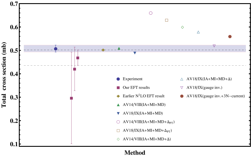
Figure 3: Comparison between different theoretical results for the total cross section of the $nd\rightarrow$ ${}^{3}H\gamma$ process. The points from left to right denote the results computed by experiment Jurney et al , our LO EFT($\pi\!\!\!/$), our NLO EFT($\pi\!\!\!/$), our $\textrm{N}^{2}\textrm{LO}$ EFT($\pi\!\!\!/$), earlier $\textrm{N}^{2}\textrm{LO}$ EFT($\pi\!\!\!/$) sadeghi-bayegan-grieshammer , AV14/VIII(IA+MI+MD) viviani et al , AV18/IX(IA+MI+MD) viviani et al , AV14/VIII(IA+MI+MD+$\Delta_{PT}$) viviani et al , AV18/IX(IA+MI+MD+$\Delta_{PT}$) viviani et al , AV14/VIII(IA+MI+MD+$\Delta$) viviani et al , AV18/IX(IA+MI+MD+$\Delta$) viviani et al , AV18/IX(gauge inv.) Marcucci et al , and AV18/IX(gauge inv.+$3N$-current) Marcucci et al methods, respectively. The thin band indicates the error band of the experimental result of the cross section. Two horizontal dashed lines determine the upper and lower limits due to our systematic EFT($\pi\!\!\!/$) error at $\textrm{N}^{2}\textrm{LO}$.

Our results in Table 1 show the convergence in our power counting from LO to $\textrm{N}^{2}\textrm{LO}$. At NLO, 0.124 mb adds to the leading-order value and at $\textrm{N}^{2}\textrm{LO}$ 0.048 mb to the next-to-leading order. Our EFT result for the total cross section of neutron radiative capture by a deuteron at $\textrm{N}^{2}\textrm{LO}$, $\sigma_{tot}^{(2)}=0.469$ mb, has an error of 7$\%$ compare with the experimental value, $\sigma_{tot}^{exp}=0.508\pm 0.015$ mb. We stress that the contribution of the E2 transition has not been included in our calculation for the amplitude of the $nd\rightarrow$ ${}^{3}H\gamma$ reaction. The E2 transition is suppressed by two powers of the initial nucleon momentum or photon energy compared to the dominant M1 transition. Therefore, this effect numerically has a contribution of $(\frac{(E_{i}-E_{f})\;\textrm{or}\;k}{\Lambda})^{2}\sim 0.25\%$ correction in the quartet-initial-channel amplitude of $nd\rightarrow$ ${}^{3}H\gamma$ and so $\sim 0.5\%$ in total cross section at threshold regime. Also, with respect to the power counting as discussed above, we expect a maximum error $\thicksim 7\%$ in $\textrm{N}^{2}\textrm{LO}$ EFT($\pi\!\!\!/$) results of the cross section. Thus the 7$\%$ error in our $\textrm{N}^{2}\textrm{LO}$ results is acceptable. We believe that the higher-order corrections make this discrepancy narrow.

Table 2: The cutoff variation of our EFT($\pi\!\!\!/$) results for the total cross section between $\Lambda=200$ and $\Lambda=900$ MeV. $n=0,1,2$ denote the LO, NLO and $\textrm{N}^{2}\textrm{LO}$ results, respectively.

$\qquad n\qquad$	Abs[$1-\frac{\sigma^{(n)}_{tot}(\Lambda=200\,\textrm{MeV})}{\sigma^{(n)}_{tot}(\Lambda=900\,\textrm{MeV})}$]
$0$	0.098756
$1$	0.045714
$2$	0.004006

According to Table 2, we have computed the cutoff variation of our EFT($\pi\!\!\!/$) results for the total cross section within a natural range of $\Lambda=200$ to $\Lambda=900$ MeV at LO, NLO, and $\textrm{N}^{2}\textrm{LO}$. The range of cutoff variation should be a few times the pion mass because, here, the existence of a definite $\Lambda\rightarrow\infty$ limit in an EFT calculation does not guarantee that the results found in that limit are rigorous consequences of the EFT Epelbanm ; Ji-Phillips . Our results in Table 2 indicate that the M1 amplitudes and the cross section of $nd\rightarrow$ ${}^{3}H\gamma$ are cutoff independent and properly renormalized.

The differences of our results and the previous EFT($\pi\!\!\!/$) calculation of total cross section at thermal energy sadeghi-bayegan-grieshammer are due to the ignored diagrams and the ${}^{3}S_{1}\rightarrow^{3}$$S_{1}$ M1 transition effects.

Table 3: The ${}^{3}S_{1}\rightarrow^{3}$$S_{1}$ M1 transition effect in the total cross section at LO ($n=0$), NLO ($n=1$) and $\textrm{N}^{2}\textrm{LO}$ ($n=2$).

$\;n\;$	$\qquad\sigma_{tot}^{(n)}\>(L_{2}=0)\qquad$	$\quad\sigma_{tot}^{(n)}\>(L_{2}=-0.4\;\textrm{fm})\quad$	difference
$0$	$0.297\pm 0.196$	$0.297\pm 0.196$	0
$1$	$0.472\pm 0.104$	$0.421\pm 0.093$	$0.051$
$2$	$0.553\pm 0.041$	$0.469\pm 0.033$	$0.084$

The $L_{2}$ coefficient corresponding to the contribution of the ${}^{3}S_{1}\rightarrow^{3}$$S_{1}$ M1 transition is small compared with $L_{1}$ which comes from the ${}^{1}S_{0}\rightarrow^{3}$$S_{1}$ M1 transition Ando-Hyun . So, we expect that the ${}^{3}S_{1}\rightarrow^{3}$$S_{1}$ M1 transition has a small (and negligible) effect at NLO results but at $\textrm{N}^{2}\textrm{LO}$ the ${}^{3}S_{1}\rightarrow^{3}$$S_{1}$ M1 transition could have a significant effect. Our results for the total cross section with and without the $L_{2}$ coefficient effect which are summarized in Table 3 are as we expected.

Table 4: The investigation of the ignored contributions in the previous EFT($\pi\!\!\!/$) calculation sadeghi-bayegan-grieshammer at each order. $\bar{\mathcal{M}}^{(n)}_{x}$ indicates the total $\textrm{N}^{n}\textrm{LO}$ amplitude of M1 $nd\rightarrow$ ${}^{3}H\gamma$ without the contribution of the time ordering that corresponds to the photon emitted during the nucleon exchange in the first diagram of the second line in Fig.1. $\mathcal{M}^{(n)}_{013,x}$ denotes the sum of the amplitudes of the diagrams ”$a_{0}$”, ”$a_{1}$”, and ”$a_{3}$” for the incoming $x$ channel. Also, $\mathcal{M}^{(n)}_{2,x}$ is only the contribution of the ”$a_{2}$” diagram in the first line of Fig.1 for the initial $x$ channel, respectively. $q$ and $d$ in the first column indicate the initial quartet (⁴$S_{\frac{3}{2}}$) and doublet (²$S_{\frac{1}{2}}$) channels, respectively. The results of the amplitudes are presented in units of $10^{-7}\;\textrm{MeV}^{-\frac{5}{2}}$.

$\;\;x\;\;$	$\;\;n\;\;$	$\qquad\sqrt{|\mathcal{M}^{(n)}_{x}|^{2}}\qquad$	$Abs\Big{[}\sqrt{|\mathcal{M}^{(n)}_{x}|^{2}}-\sqrt{|\bar{\mathcal{M}}^{(n)}_{x}|^{2}}\Big{]}$	$\quad\sqrt{|\mathcal{M}^{(n)}_{013,x}|^{2}}\quad$	$\quad\sqrt{|\mathcal{M}^{(n)}_{2,x}|^{2}}\quad$
	$0$	$4.88\pm 1.61$	$0.10$	$5.27$	$0.21$
$q$	$1$	$5.20\pm 0.57$	$0.47$	$6.05$	$0.42$
	$2$	$5.30\pm 0.19$	$0.90$	$6.26$	$0.58$
	$0$	$3.65\pm 1.20$	$2.11$	$3.79$	$1.16$
$d$	$1$	$5.68\pm 0.63$	$2.94$	$4.37$	$2.41$
	$2$	$6.33\pm 0.23$	$3.47$	$4.55$	$3.39$

The effects of the diagrams in Fig.1 which have been neglected in the previous EFT($\pi\!\!\!/$) calculation sadeghi-bayegan-grieshammer have been investigated in Table 4. The results in the third column of Table 4 are the total doublet and quartet amplitudes of the M1 $nd\rightarrow$ ${}^{3}H\gamma$ transition at LO, NLO and $\textrm{N}^{n}\textrm{LO}$. In the fourth column, we present the computed values of the contribution which is only corresponding to the nucleon pole before photon creation in the first diagram in the second line of Fig.1 at each order. The fifth and sixth columns of Table 4 represent only the evaluated values for the amplitudes of the ”$a_{0}+a_{1}+a_{3}$” and ”$a_{2}$” diagrams in the first line of Fig.1, respectively, for both doublet and quartet channels.

The lack of a correct calculation of the first diagram of the second line in Fig.1 creates the significant errors as indicated in the fourth column of Table IV at each order. The results shown in the fifth column of Table 4 indicate that the diagrams with radiation from external nucleon leg, external deuteron leg, and on-shell two-body bubble in the first line of Fig.1 are LO effects and so, one expects that these diagrams have a very important effect in the final results of the amplitude of the M1 $nd\rightarrow$ ${}^{3}H\gamma$ transition and could not be ignored. But the last column depicts that the diagram ”$a_{2}$” in the first line of Fig.1 has a small effect at LO especially in the quartet channel as estimated in the previous EFT($\pi\!\!\!/$) calculation sadeghi-bayegan-grieshammer . Finally, we emphasize that our results have been evaluated using the properly normalized triton wave function.

VI Conclusion and Outlook

In the present parity-conserving EFT($\pi\!\!\!/$) calculation, we have calculated the amplitudes and cross section for $nd\rightarrow$ ${}^{3}H\gamma$ fully in the cluster-configuration space up to $\textrm{N}^{2}\textrm{LO}$. We have considered one- and two-body currents. No three-body currents are needed to renormalize the observables in this work up to $\textrm{N}^{2}\textrm{LO}$. The M1 is the dominant transition at the low energies. We have included the contribution of the possible diagrams which have not been included in the previous EFT($\pi\!\!\!/$) calculations and used the properly normalized triton wave function. We have also considered the effects of the ${}^{3}S_{1}\rightarrow^{3}$$S_{1}$ M1 transition ($L_{2}$ coefficient in Eq.(3)) in the $nd\rightarrow$ ${}^{3}H\gamma$ amplitudes together with other transitions which are included in the previous EFT($\pi\!\!\!/$) calculations.

The $\textrm{N}^{2}\textrm{LO}$ EFT($\pi\!\!\!/$) total cross section is determined to be $\sigma^{(2)}_{tot}=0.469\pm 0.033$ mb. The reliable calculation of the doublet and quartet amplitudes can be used in the calculation of parity-violating observables in the $nd\rightarrow$ ${}^{3}H\gamma$ process. The $\textrm{N}^{2}\textrm{LO}$ EFT($\pi\!\!\!/$) total cross section $\sigma_{tot}^{(2)}$ is within 7$\%$ of the measured values. The remaining discrepancies between theory and experiment indicate that inclusion of 1) higher order corrections and 2) higher-order multipoles contributions, may refine the differences.

Appendix A Faddeev Equations of $Nd$ scattering in the Doublet and Quartet channels

The diagrams of the $Nd$ scattering amplitude up to $\textrm{N}^{n}\textrm{LO}$ are shown in Fig.4. The Faddeev equation of the diagrams in Fig.4 for the quartet channel in the cluster-configuration space is given by

$$\left(\begin{array}[]{cc}t^{(n)}_{q}(E;k,p)&0\\ 0&0\\ \end{array}\right)=-4\pi\mathcal{K}(E;k,p)\left(\begin{array}[]{cc}1&0\\ 0&0\\ \end{array}\right)\qquad\qquad\qquad\qquad\qquad\qquad\quad$$ (57)

$$+\frac{2}{\pi}\int^{\Lambda}_{0}dq\>q^{2}\>\mathcal{K}(E;q,p)\mathcal{D}^{(n)}(E,q)\left(\begin{array}[]{cc}t^{(n)}_{q}(E;k,p)&0\\ 0&0\\ \end{array}\right).\>$$ (60)

and for the $Nd$ scattering in the doublet ($S$=$\frac{1}{2}$) channel, we have

$$\left(\begin{array}[]{cc}t^{(n)}_{d_{d_{t}N\rightarrow d_{t}N}}&t^{(n)}_{d_{d_{s}N\rightarrow d_{t}N}}\\ t^{(n)}_{d_{d_{t}N\rightarrow d_{s}N}}&t^{(n)}_{d_{d_{s}N\rightarrow d_{s}N}}\\ \end{array}\right)(E;k,p)=2\pi\left[\mathcal{K}(E;k,p)\left(\begin{array}[]{cc}1&-3\\ -3&1\\ \end{array}\right)+\mathcal{H}(E,\Lambda)\left(\begin{array}[]{cc}1&-1\\ -1&1\\ \end{array}\right)\right]\;$$ (67)

$$-\frac{1}{\pi}\int^{\Lambda}_{0}dqq^{2}\left[\mathcal{K}(E;q,p)\left(\begin{array}[]{cc}1&-3\\ -3&1\\ \end{array}\right)+\mathcal{H}(E,\Lambda)\left(\begin{array}[]{cc}1&-1\\ -1&1\\ \end{array}\right)\right]$$ (72)

$$\times\mathcal{D}^{(n)}(E,q)\left(\begin{array}[]{cc}t^{(n)}_{d_{d_{t}N\rightarrow d_{t}N}}&t^{(n)}_{d_{d_{s}N\rightarrow d_{t}N}}\\ t^{(n)}_{d_{d_{t}N\rightarrow d_{s}N}}&t^{(n)}_{d_{d_{s}N\rightarrow d_{s}N}}\\ \end{array}\right)(E;k,q),\qquad\qquad\;\>$$ (75)

where $E=\frac{3k^{2}}{4m_{N}}-\frac{\gamma^{2}_{t}}{m_{N}}$, $k$ and $p$ are the total energy of $Nd$ system, the incoming and outgoing momentums, respectively.

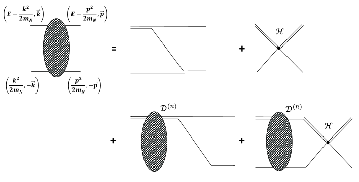
Figure 4: The $Nd$ scattering diagrams up to $\textrm{N}^{n}\textrm{LO}$ ($n\leq 2$). All notations are the same as in Fig.1.

In Eq.(67), $t^{(n)}_{d_{d_{x}N\rightarrow d_{y}N}}$ denotes the $d_{x}N\rightarrow d_{y}N$ transition amplitude ($x,y=s$ or $t$) in the doublet channel. The propagator of the exchanged nucleon, $\mathcal{K}$, is

$$\!\mathcal{K}(E;k,p)=\frac{1}{2}\int^{1}_{-1}\frac{d(cos\,\theta)}{\!k^{2}\!+p^{2}-ME+kp\>\textrm{cos}\,\theta},$$ (76)

where $\theta$ indicates the angle between $\vec{k}$ and $\vec{p}$ vectors. Other variables in the above equation are similar to the text. The results of Eqs.(57) and (67) are evaluated by considering the operators for projecting the $Nd$ system to ${}^{2}S_{\frac{1}{2}}$ and ${}^{4}S_{\frac{3}{2}}$ channels. For the doublet and quartet channels the projection operators $\mathcal{P}_{d,iA}$ and $\mathcal{P}^{j}_{q,i}$ are used, respectively, with iso-spin index $A$ and spin indices $i$ and $j$ 20 of sadeghi-bayegan .

Appendix B Triton Wave function

The normalized triton wave function is obtained by solving the homogeneous part of Eq.(67) with the application of $E=-B_{t}$, where $B_{t}$ is the binding energy of the triton. So, the homogeneous part of Eq.(67) for the calculation of the triton wave function up to $\textrm{N}^{n}\textrm{LO}$ can be written as

$$t^{(n)}_{{}^{3}H}(p)=-\frac{1}{\pi}\int^{\Lambda}_{0}dqq^{2}\Bigg{[}\mathcal{K}(-B_{t};q,p)\left(\begin{array}[]{cc}1&-3\\ -3&1\\ \end{array}\right)\qquad\qquad\qquad\qquad\quad\;$$ (79)

$$+\mathcal{H}(-B_{t},\Lambda)\left(\begin{array}[]{cc}1&-1\\ -1&1\\ \end{array}\right)\Bigg{]}\mathcal{D}^{(n)}(-B_{t},q)\,t^{(n)}_{{}^{3}H}(q),$$ (82)

where $t^{(n)}_{{}^{3}H}(q)=\bigg{(}\begin{array}[]{cc}t^{(n)}_{{}^{3}H_{d_{t}N\rightarrow d_{t}N}}(q)&t^{(n)}_{{}^{3}H_{d_{s}N\rightarrow d_{t}N}}(q)\\ t^{(n)}_{{}^{3}H_{d_{t}N\rightarrow d_{s}N}}(q)&t^{(n)}_{{}^{3}H_{d_{s}N\rightarrow d_{s}N}}(q)\\ \end{array}\bigg{)}$. Generally, $t^{(n)}_{{}^{3}H_{d_{x}N\rightarrow d_{y}N}}(q)$ denotes the contribution of the ${d_{x}N\rightarrow d_{y}N}$ transition ($x,y=s$ or $t$) for making the triton.

One can be able to normalize the solution of Eq.(79) for the incoming deuteron channel by moeini-bayegan

$$1=-\int\frac{q^{2}\,dq}{2\pi^{2}}\int\frac{q^{\prime 2}\,dq^{\prime}}{2\pi^{2}}\big{(}t^{(n)}_{{}^{3}H}(q)\bigg{(}\begin{array}[]{cc}1\\ \,0\end{array}\bigg{)}\big{)}^{\dagger}\mathcal{D}^{(n)}(-B_{t},q)\qquad\qquad\qquad\quad\;\;\;$$ (85)

$$\times\frac{\partial}{\partial E}\Big{[}V(E,q,q^{\prime})\mathcal{D}^{(n)}(E,q^{\prime})\Big{]}\bigg{|}_{E=-B_{t}}\!\!\!t^{(n)}_{{}^{3}H}(q^{\prime})\bigg{(}\begin{array}[]{c}1\\ 0\end{array}\bigg{)},$$ (88)

where $V$ is given by

$$V(E,q,q^{\prime})=2\pi\left[\mathcal{K}(E;q,q^{\prime})\bigg{(}\begin{array}[]{cc}1&-3\\ -3&1\\ \end{array}\bigg{)}+\mathcal{H}(E,\Lambda)\bigg{(}\begin{array}[]{cc}1&-1\\ -1&1\\ \end{array}\bigg{)}\right].$$ (93)

If we need to find the normalized contribution of the triton wave function which comes from the incoming singlet dibaryon field, the replacement $\bigg{(}\begin{array}[]{c}1\\ 0\end{array}\bigg{)}$ by $\bigg{(}\begin{array}[]{c}0\\ 1\end{array}\bigg{)}$ in Eq.(85) must be done.

References

• (1) G. Rupak, Nucl. Phys. A 678, 405 (2000).
• (2) H. Sadeghi, and S. Bayegan, Nucl. Phys. A 753, 291 (2005).
• (3) H. Sadeghi, S. Bayegan, and H. W. Grießhammer, Phy. Lett. B 643, 263 (2006). [arXiv:nucl-th/0610029]
• (4) G. Rupak, and R. Higa, Phys. Rev. Lett. 106, 222501 (2011).
• (5) H. -W. Hammer, and D. R. Phillips, Nucl. Phys. A 865, 17 (2011).
• (6) B. Acharya, and D. R. Phillips, Nucl. Phys. A 913, 103 (2013).
• (7) A. N. Moskalev, Yad. Fiz. 9, 163 (1969); Sov. J. Nucl. Phys. 9, 99 (1969).
• (8) B. Desplanques and J. J. Benayoun, Nucl. Phys. A 458, 689 (1986).
• (9) M. M. Arani, and S. Bayegan, Euro. Phys. J. A 49, 117 (2013).
• (10) H. W. Grießhammer, Nucl. Phys. A 744, 192 (2004).
• (11) J. Adam, F. Gross, C. Savkli, and J. W. Van Orden, Phys. Rev. C 56, 641 (1997).
• (12) F. Gross, Relativistic Quantum Mechanics and Field Theory, (Wiley-Interscience, New York,1993).
• (13) G. Faldt, and L. G. Larsson, J. Phys. G: Nucl. Part. Phys. 19, 569 (1993).
• (14) M. Viviani, R. Schiavilla, and A. Kievsky, Phys. Rev. C 54, 534 (1996).
• (15) E. T. Jurney, P. J. Bendt, and J. C. Browne, Phys. Rev. C 25, 2810 (1982).
• (16) L. Kaplan, G. R. Ringo, and K. E. Wilzbach, Phys. Rev. 87, 785 (1952).
• (17) J. S. Merritt, J. G. V. Taylor, and A. W. Boyd, Nucl. Sci. Eng. 34, 195 (1968).
• (18) D. R. Phillips, G. Rupak, and M. J. Savage, Phys. Lett. B 473, 209 (2000).
• (19) P. F. Bedaque, G. Rupak, H. W. Grießhammer, and H. -W. Hammer, Nucl. Phys. A 714, 589 (2003).
• (20) S. I. Ando, and Ch. H. Hyun, Phys. Rev. C 72, 014008 (2005).
• (21) H. W. Grießhammer, Few. Body. Syst. 44, 137 (2008).
• (22) J. H. Hetherington, and L. H. Schick, Phys. Rev. B 137, 935 (1965).
• (23) R. T. Cahill, and I. H. Sloan, Nucl. Phys. A 165, 161 (1971).
• (24) R. Aaron, and R. D. Amado, Phys. Rev. 150, 857 (1966).
• (25) P. F. Bedaque, H. -W. Hammer, and U. van Kolck, Phys. Rev. Lett. 82, 463 (1999); Nucl. Phys. A 646, 444 (1999).
• (26) P. F. Bedaque, H. -W. Hammer, and U. van Kolck, Nucl. Phys. A 676, 357 (2000).
• (27) L. E. Marcucci, M. Viviani, R. Schiavilla, A. Kievsky, and S. Rosati, Phys. Rev. C 72, 014001 (2005).
• (28) E. Epelbaum and J. Gegelia, Eur. Phys. J. A 41, 341 (2009).
• (29) Ch. Ji and D. R. Phillips, Few. Body. Syst. 54, 2317 (2013).