Entropy for Quantum Pure States and Its Dynamical Relaxation

Abstract

We construct a complete set of Wannier functions which are localized at both given positions and momenta. This allows us to introduce the quantum phase space, onto which a quantum pure state can be mapped unitarily. Using its probability distribution in quantum phase space, we define an entropy for a quantum pure state. We prove an inequality regarding the long time behavior of our entropy’s fluctuation. For a typical initial state, this inequality indicates that our entropy can relax dynamically to a maximized value and stay there most of time with small fluctuations. This result echoes the quantum H-theorem proved by von Neumann in [Zeitschrift für Physik 57, 30 (1929)]. Our entropy is different from the standard von Neumann entropy, which is always zero for quantum pure states. According to our definition, a system always has bigger entropy than its subsystem even when the system is described by a pure state. As the construction of the Wannier basis can be implemented numerically, the dynamical evolution of our entropy is illustrated with an example.

I Introduction

Statistical mechanics, studying thermal properties of a many-body system from microscopic perspective, have gained huge success in the past century. However, the basic principles of statistical mechanics have not been fully understood; the establishment of micro-cannonical ensemble has to rely on hypothesesHuang (1987). Since microscopic particles — elements of a macroscopic system — are governed by the Schrödinger equation, one feels obliged to address the problem with quantum mechanics. Von Neumann was among the first physicists trying to use quantum mechanics to understand the basic principles of statistical mechanics. In a 1929 papervon Neumann (1929), von Neumann proposed a method to construct commutable macroscopic momentum and position operators and, therefore, quantum phase space. Within this framework, he introduced an entropy for quantum pure state and proved two theorems, which he called quantum ergodic theorem and quantum H-theorem, respectively. These results are remarkable advances in the establishment of the micro-canonical ensemble, the foundation of statistical mechanics, without hypothesis. However, von Neumann’s beautiful results have been largely forgotten likely due to misunderstandingGoldstein et al. (2010a).

Probably due to the developments in ultra-cold atomic gas experimentsKinoshita et al. (2006); Smith et al. (2013); Yukalov (2011a), we have recently seen tremendous efforts to study the foundation of statistical mechanics. Many new and beautiful results are obtained Gemmer et al. (2004); Srednicki (1994); Goldstein et al. (2006); Popescu et al. (2006); Dong et al. (2007); Rigol et al. (2008); Goldstein et al. (2010b); Linden et al. (2009); Reimann (2007, 2008); Reimann and Kastner (2012); Cho and Kim (2010); Ikeda et al. (2011); Ji and Fine (2011); Yukalov (2011b); Sugiura and Shimizu (2012); Snoke et al. (2012); Wang (2012); Rigol and Srednicki (2012); Riera et al. (2012); Ududec et al. (2013); Zhuang and Wu (2014); Goldstein et al. (2014). These efforts have also led to renewed interest in von Neumann’s forgotten work; the English version of his paper is now available Neumann (2010). Von Neumann’s quantum ergodic theorem has been re-exmained recentlyGoldstein et al. (2010c). In particular, a different version of quantum ergodic theorem was proved by Reimann Reimann (2008); Short (2011). Reimann’s ergodic theorem does not involve any coarse-graining and can be subjected to numerical studyZhuang and Wu (2013). In contrast, much less progress has been made on the quantum H-theorem and the associated key concepts, such as macroscopic momentum and position operators, and entropy for quantum pure states, which were introduced in 1929.

In this work we define a different entropy for quantum pure states and study its long-time dynamical fluctuation in attempt to improve on von Neumann’s quantum H-theoremvon Neumann (1929). Von Neumann proved his theorem with the following steps: (i) construct commutable macroscopic position and momentum operators; (ii) define an entropy for pure quantum states with coarse-graining; (iii) investigate the long-time behavior of the entropy.

We follow von Neumann’s steps with new theoretical tools and perspectives. For step (i), we use Kohn’s method Kohn (1973) to construct a complete set of Wannier functions that are localized both in position and momentum space. Such a construction can be implemented numerically with great efficiency. With these Wannier functions, we are able to construct commutable macroscopic position and momentum operators and, therefore, a quantum phase space, which is divided into cells of size of the Planck constant and each of these Planck cells is assigned a Wannier function. The success of step (i) allows us to map unitarily a pure quantum state onto the phase space.

We accomplish step (ii) by defining an entropy for a quantum pure state based on its probability distribution on the phase space. Here we do not use coarse-graining used by von Neumann in the context of macroscopic observables. For our entropy, the total system always has a larger entropy than its subsystems even if the total system is described by a quantum pure state. This is not the case for the conventional von Neumann’s entropy for mixed states.

For step (iii), we introduce an ensemble entropy for a pure state and prove an inequality regarding the dynamical fluctuation of our entropy, which is similar to von Neumann’s quantum H-theorem. This inequality includes a constant $C$ that characterizes the correlation of probability fluctuations between different Planck cells. When the correlation is small, the inequality dictates that our entropy relax dynamically to the ensemble entropy and stay at this value most of time with small fluctuations for macroscopic systems. Our analysis shows that $C$ is small as long as the energy shell of microcanonical ensemble is not too narrow and not sporadically populated. As a result, a better understanding of the microscopic origin of the second law of thermodynamics is achieved. The long-time dynamical evolution of our entropy is illustrated numerically with an example.

II Quantum phase space

To establish quantum phase space, von Neumann proposed to construct a macroscopic position operator $\bm{Q}$ and a macroscopic momentum operator $\bm{P}$ that satisfyNeumann (2010)

$$[\bm{Q},\bm{P}]=0\,,$$ (1)

$$\bm{Q}\sim\bm{q},\quad\bm{P}\sim\bm{p}\,,$$ (2)

where $\bm{q}$ and $\bm{p}$ are usual microscopic position and momentum operators, respectively, that have the commutator $[\bm{q},\bm{p}]=i\hbar$. Eq. (2) indicates that the macroscopic position and momentum operators are not identical but close to their microscopic counterparts. Mathematically it is equivalent to finding a complete set of normalized orthogonal wave functions $\{\mathit{w}_{j}\}$ localized in both position and momentum spaces. The macroscopic position and momentum operators can then be expressed as

$$\bm{P}=\sum_{j}|\mathit{w}_{j}\rangle\langle\mathit{w}_{j}|\bm{p}|\mathit{w}_{j}\rangle\langle\mathit{w}_{j}|\,,$$ (3)

$$\bm{Q}=\sum_{j}|\mathit{w}_{j}\rangle\langle\mathit{w}_{j}|\bm{q}|\mathit{w}_{j}\rangle\langle\mathit{w}_{j}|\,.$$ (4)

Eq. (2) implies that the $i^{\textrm{th}}$ order central moments

$$\Delta^{(i)}p_{j}\equiv\langle\mathit{w}_{j}|(\bm{p}-\langle\bm{p}\rangle_{j})^{i}|\mathit{w}_{j}\rangle^{1/i}$$ (5)

$$\Delta^{(i)}q_{j}\equiv\langle\mathit{w}_{j}|(\bm{q}-\langle\bm{q}\rangle_{j})^{i}|\mathit{w}_{j}\rangle^{1/i}$$ (6)

should be relatively small for all $i\geq 2$. $\langle f\rangle_{j}$ denotes $\langle w_{j}|f|w_{j}\rangle$. For convenience, we often denote $\Delta^{(2)}$ simply by $\Delta$.

For one-dimensional system in which $\bm{q}\equiv\bm{x}$, $\bm{p}\equiv\hbar\bm{k}=-i\hbar\partial_{x}$, von Neumann proposed to find $\{\mathit{w}_{j}\}$ by Schmidt orthogonalizing a set of Gaussian wave packets of width $\zeta$von Neumann (1929)

$$g_{j_{x},j_{k}}\equiv\exp\big{[}-\frac{(x-j_{x}x_{0})^{2}}{4\zeta^{2}}+ij_{k}k_{0}x\big{]}\,,$$ (7)

where $j_{x},j_{k}$ are integers. When $x_{0}\,k_{0}=2\pi$, this set of Gaussian packets are complete. We are at liberty to choose $x_{0}$, $k_{0}$, and $\zeta$ as long as $x_{0}\,k_{0}=2\pi$ is satisfied. Unless otherwise specified, parameters are chosen as $x_{0}=1$, $k_{0}=2\pi$ and $\zeta=(2\pi)^{-1}$.

This method, which is called “cumbersome” by von Neumann himself Neumann (2010), suffers from two major drawbacks. First, it is not feasible numerically due to its high computational cost and sensitivity to the order of the orthogonalization procedure. Secondly, von Neumann argued von Neumann (1929) that the existence of $\bm{P}$ and $\bm{Q}$ corresponds to the fact that the position and momentum can be measured simultaneously in macroscopic measurements. As there is no difference among measuring positions at different spatial points, we expect that the constructed $\{\mathit{w}_{j}\}$ have spatial translational symmetry. However, the wave packets constructed with von Neumann’s method have no such symmetry.

II.1 Wannier Basis

Kohn suggested a method to construct Wannier functions out of Gaussian wave packets Kohn (1973). We adapt Kohn’s approach to orthogonalize the Gaussian packets in Eq.(7) and construct a complete set of Wannier functions $\{\mathit{w}_{j}\}$ whose translational symmetry is guaranteed. The detailed procedure of construction is elaborated as follows.

1. Choose an initial set of localized wave packets such as the Gaussian wave packets $g_{j_{k}}(x)\equiv g_{0,j_{k}}(x)$ in Eq. (7). Find their Fourier transform $\tilde{g}_{j_{k}}(k)\equiv\mathcal{F}\{g_{j_{k}}(x)\}\equiv\frac{1}{\sqrt{2\pi}}\int g_{j_{k}}(x)\mathrm{e}^{-ikx}\;\mathrm{d}x$.

2. At a fixed $k$, for every $j_{k}$, $(\tilde{g}_{j_{k}}(k+2n\pi))_{n\in\mathbb{Z}}$ is a normalizable vector; we denote it by $u_{k,j_{k}}(n)$. Apply Schmidt orthogonalization procedure $v_{0}=u_{0}$ (the subscript $k$ is omitted), normalize $v_{0}$, $v_{1}=u_{1}-(u_{1},v_{0})v_{0}$, normalize $v_{1}$, and repeat for $u_{2}$, $u_{3},\cdots$. We eventually get an orthonormal basis $\{v_{k,j_{k}}\in l^{2}(\mathbb{Z})\}_{j_{k}\in\mathbb{Z}}$. Define $\tilde{\mathit{w}}_{j_{k}}(k+2n\pi)\equiv v_{k,j_{k}}(n)/\sqrt{2\pi}$.

3. For every $k$ (discrete in numerical calculations) on $[0,2\pi)$, repeat step 2. According to Proposition 1 in Appendix A, $\mathit{w}_{j_{x},j_{k}}(x)\equiv\mathit{w}_{j_{k}}(x-j_{x})$ ($\mathit{w}_{j_{k}}$ is the Fourier transform of $\tilde{\mathit{w}}_{j_{k}}$) are orthonormal. $\{w_{j}\}$ is the desired orthonormal basis ($j=(j_{x},j_{k})$).

We have thus established a quantum phase space which is different from the classical phase space: (1) It is divided into phase cells of size Planck constant $h$ (for one dimensional system) as illustrated in Fig. 1 (a); we call such a cell Planck cell for brevity. (2) Each Planck cell is assigned a Wannier function $w_{j}$, which is localized near site ($x=j_{x}$, $k=2j_{k}\pi$). We are now able to map a pure wave function unitarily onto phase space. There has been tremendous efforts to formulate quantum mechanics in phase space based on Wigner’s quasi-distribution function and Weyl’s correspondence Zachos et al. (2005). However, Wigner’s quasi-distribution is not positive-definite and cannot be interpreted as probability in phase space. According to our construction, for a wave function $\psi$, $|\braket{\psi}{\mathit{w}_{j}}|^{2}$ is its probability at Planck cell $j$ as $\{\mathit{w}_{j}\}$ is a set of complete orthonormal basis.

The generalization to higher dimensions is straightforward. With the one-dimensional $\{\mathit{w}_{j}(x)\}$ that we have constructed, we simply define

$$\mathit{w}_{j_{1}j_{2}\ldots j_{n}}(x_{1},x_{2},\ldots,x_{n})\equiv\mathit{w}_{j_{1}}(x_{1})\mathit{w}_{j_{2}}(x_{2})\ldots\mathit{w}_{j_{n}}(x_{n})\,.$$ (8)

Then $\{\mathit{w}_{j_{1}j_{2}\ldots j_{n}}\}$ is the localized orthonormal basis for an $n$-dimensional system.

Numerical results of one-dimensional Wannier functions are provided in Fig. 1. A Wannier function localized near $(x=3,k=20\pi)$ is plotted in the $k$ and $x$ spaces, respectively, in Fig. 1(c) and (d). This Wannier function is obtained with the above procedure using the Gaussian wave packets $g_{j_{x},j_{k}}$ as initial functions. And the order of Schmidt orthogonalization in our procedure is chosen to be $j_{k}=0,1,-1,2,-2,\ldots$. The result does not sensitively depend on the order.

Our numerical computation finds that the Wannier function spreads out slowly with increasing momentum $k$. From Fig. 1 (b) we can see that both $\Delta^{(i)}k_{j}$ and $\Delta^{(i)}x_{j}$, which characterize the spreads of the Wannier function, diverge as $j_{k}$ increases; $\Delta^{(i)}x_{j}$ appears to grow more slowly. Actually, it can be proved that the product of $\Delta x_{j}\cdot\Delta k_{j}$ diverges as $j_{k}$ increases no matter what initial wave packets are chosen (see Appendix B). This divergent behavior of $\Delta x\cdot\Delta k$ is called strong uncertainty relationBourgain (1988).

However, the divergence is not very severe. As shown in Fig. 1 (b) where both axes are in logarithmic scales, all the growth slopes are much less than one. Therefore, all orders of the relative spreads $\Delta^{(i)}x_{j}/2\pi j_{k}$ and $\Delta^{(i)}k_{j}/2\pi j_{k}$ fall to zero quickly as $j_{k}$ increases. This suggests that for the one-dimensional system, the requirement (5) and (6) are satisfied in the sense

$$\lim_{\langle p\rangle_{j}/p_{0}\to\infty}\frac{\Delta^{(i)}p_{j}}{\langle p\rangle_{j}}=\lim_{\langle p\rangle_{j}/p_{0}\to\infty}\frac{p_{0}\cdot\Delta^{(i)}q_{j}}{\langle p\rangle_{j}q_{0}}=0\,,$$ (9)

where we have used $p=\hbar k$, $q=x$, and $\langle p\rangle_{j}\approx j_{k}p_{0}$.

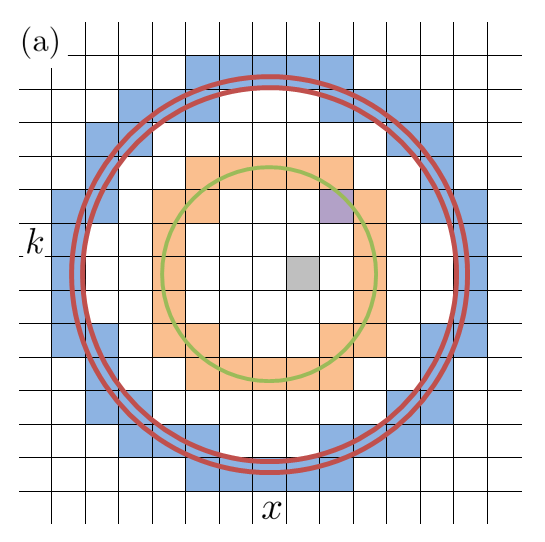
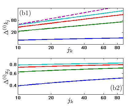
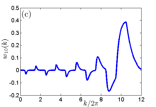
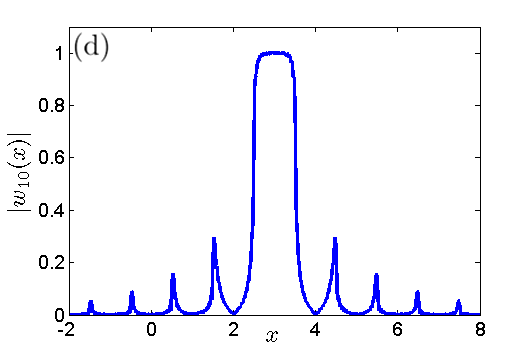
Figure 1: Illustration of quantum phase space. (a) Schematic plot of quantum phase space (b) Spreads of Wannier functions as a function of $j_{k}$. Both axes are in logarithmic scales. Solid lines are for $i=8,6,4,2$, from top to bottom, respectively. The dashed line of slope 1 is drawn to show that all solid lines have slope less than 1. (c) Wannier function $\mathit{w}_{3,10}$ is shown localized near $k=10\cdot 2\pi$. (d) Wannier function $\mathit{w}_{3,10}$ is shown localized near $x=3$.

II.2 Quantum Energy Shell

In classical phase space, there is an important concept of energy surface, where the dynamics of an isolated system is confined. Energy surface, which is of no width, is no longer valid in the quantum phase space which consists of cells of finite size. However, a similar concept, energy shell of finite width, can be introduced. For this purpose, we need to first show that each of our Planck cells is localized in energy for most of the macroscopic systems of physical interest.

For an isolated system of fixed number of particles $N\gg 1$ with Hamiltonian $H(\bm{p},\bm{r})$ where $\bm{p}$ and $\bm{r}$ are $3N$-dimensional vectors, define $p_{C}$ as the typical magnitude of momentum of any particle and $r_{C}$ as the typical length scale on which $H$ changes relatively significantly. For example, $r_{C}$ can be the mean free path of a particle or the characteristic scale of the external potential. We define the index

$$I\equiv p_{C}r_{C}/h$$ (10)

In this work we focus on the cases where $I$ is considerably large.

We expect that the quantum phase space is reduced to the classical phase space in the limit $I\to\infty$ in the sense that the relative size of a Planck cell and the relative spreads of the Wannier functions tend to zero. This is indeed the case. We construct Planck cells defined by $p_{0}=p_{C}/\sqrt{I}$ and $r_{0}=r_{C}/\sqrt{I}$. We immediately have $p_{0}/p_{C}=r_{0}/r_{C}=I^{-1/2}\to 0$ in the limit $I\to\infty$. Suppose that $j_{C}$ is the momentum index such that $\langle p\rangle_{j_{C}}\approx p_{C}$. For a typical Planck cell $j$ whose $|j_{k}|\lesssim j_{C}$, we have according to Eq. (9)

$$\frac{\Delta^{(i)}p_{j}}{p_{C}}\lesssim\frac{\Delta^{(i)}p_{j_{C}}}{p_{C}}\to 0\,,$$ (11)

and similarly,

$$\frac{\Delta^{(i)}r_{j}}{r_{C}}=\frac{p_{0}}{r_{0}}\frac{\Delta^{(i)}r_{j}}{p_{C}}\lesssim\frac{p_{0}}{r_{0}}\frac{\Delta^{(i)}r_{j_{C}}}{p_{C}}\to 0\,,$$ (12)

for $i=2,3,\dots$ in the limit $I\to\infty$. We obtain the desirable picture, the quantum phase space becoming the classical phase space as $I\to\infty$. We thus call $I\to\infty$ classical limit. We will continue to use this choice of $p_{0}$ and $r_{0}$ in the following discussion.

Now we are ready to show that indeed our Wannier functions are localized in energy. To avoid cumbersome partial derivatives and summations, we illustrate the point with single-particle one-dimensional potential $V(x)$; the case of kinetic energy and multi-particle systems should be essentially the same. For a typical Planck cell $j$, we expand $V$ at $\langle x\rangle_{j}$ where $|w_{j}\rangle$ is localized and compute its relative spread

$$\frac{\Delta V^{2}}{V_{0}^{2}}=\left\langle\frac{(V-V_{0})^{2}}{V_{0}^{2}}\right\rangle_{j}=\sum_{i=2}^{\infty}a_{j,i}\left(\frac{\Delta^{(i)}x_{j}}{r_{C}}\right)^{i}$$ (13)

where $V_{0}\equiv V(\langle x\rangle_{j})$. As $V$ varies on the scale $r_{C}$ , it is easy to see that $a_{j,i}=O(1)$. Therefore, the relative spread $\Delta V^{2}/V_{0}^{2}$ tends to zero in the classical limit $I\to\infty$.

As our Wannier functions are localized in energy, when we map an energy eigenstate $\ket{\phi_{\alpha}}$ with eigen-energy $E_{\alpha}$ to the quantum phase space, only the Planck cells with their energies $E_{j}=\braket{w_{j}}{H}{w_{j}}\sim E_{\alpha}$ are significantly occupied. We say that energy eigenstate $\ket{\phi_{\alpha}}$ crosses Planck cell $j$ when $\langle w_{j}|\phi_{\alpha}\rangle$ is significantly non-zero. As a result, we can define an energy shell $a$ of energy interval $[E_{a},E_{a}+\Delta E_{a}]$ as a set of phase cells $\mathit{w}_{j}$’s such that $\langle\phi_{\alpha}|\bm{\Delta}_{a}|\phi_{\alpha}\rangle\sim 1$ when $E_{\alpha}\in[E_{a},E_{a}+\Delta E_{a}]$. The projection operator $\bm{\Delta}_{a}\equiv\sum_{j=1}^{N_{a}}|\mathit{w}_{j}\rangle\langle\mathit{w}_{j}|$, where $N_{a}=\,\mathrm{tr}\,\bm{\Delta}_{a}$ is the number of Planck cells in energy shell $a$. Energy shell $a$ is said to be significantly occupied by a quantum state $\psi(t)$ when $\overline{\langle\psi(t)|\bm{\Delta}_{a}|\psi(t)\rangle}$ is considerably larger than zero.

We draw the quantum phase space schematically in Fig. 1(a), where squares are for Planck cells and circles represent eigen-energies. Two energy shells are illustrated: one with blue Planck cells and the other with orange Planck cells. Each energy eigenstate may cross many Planck cells; at the same time, one Planck cell can be crossed by many energy eigenstates. The purple Planck cell is in the orange energy shell while the gray one is in neither shell colored.

III Hierarchy of Energy Scales

In this section we examine the energy scales involved and establish a hierarchy among them. It will become clear later that these energy scales and their hierarchy play crucial roles in regulating the long time dynamics of the system.

One energy scale is $\Delta_{\textrm{E}}E$, the typical difference between adjacent eigen-energies. The typical energy uncertainty $\Delta_{\textrm{Q}}E$ in a Planck cell is another energy scale. For a typical Planck cell $j$, we have

$$\Delta_{\textrm{Q}}E=\big{[}\sum_{\alpha}(E_{\alpha}-E_{j})^{2}|\langle w_{j}|\phi_{\alpha}\rangle|^{2}\big{]}^{\frac{1}{2}}\,.$$ (14)

For a quantum system with large number of particles $N\gg 1$, it should be expected that though $w_{j}$’s are localized in energy, eigenstates that cross every Planck cell are numerous. To see this, we note that the density of state $\rho(E)$ grows exponentially while $\Delta_{\textrm{Q}}E$ increases polynomially as $N\to\infty$. Therefore, for a typical many-particle system, we have $\Delta_{\textrm{E}}E\ll\Delta_{\textrm{Q}}E$.

Consider a general quantum state $\ket{\psi(t)}=\sum_{\alpha}c_{\alpha}(t)\ket{\phi_{\alpha}}\,,$ and denote $\wp_{\alpha}\equiv|c_{\alpha}(t)|^{2}$. For this quantum state, there exists an energy scale $\Delta_{\textrm{C}}E$ defined as

$$\Delta_{\textrm{C}}E=\big{[}\sum_{j,\alpha}(E_{\alpha}-E_{j})^{2}\wp_{\alpha}|\langle w_{j}|\phi_{\alpha}\rangle|^{2}\big{]}^{\frac{1}{2}}\,,$$ (15)

where $E_{j}\equiv\braket{w_{j}}{H}{w_{j}}$ is the average energy of Planck cell $j$. We call $\Delta_{\textrm{C}}E$ the correlation energy scale. As we will show later, only the Planck cells which are separated by energy less than $\Delta_{\textrm{C}}E$ are correlated. A comparison between Eq. (14) and Eq. (15) indicates that we have $\Delta_{\textrm{Q}}E\sim\Delta_{\textrm{C}}E$ for a typical quantum state.

Many properties, in particular macroscopic properties of a system, are not sensitive to the details of a quantum state. Since $\Delta_{\textrm{E}}E\ll\Delta_{\textrm{Q}}E$, we define a smoothed function over energy scale $\Delta_{\textrm{Q}}E$ as follows

$$\langle f_{\alpha}\rangle_{s}(E)\equiv\sum_{|E_{\alpha}-E|<\Delta_{\textrm{Q}}E}f_{\alpha}\big{/}\sum_{|E_{\alpha}-E|<\Delta_{\textrm{Q}}E}1\,,$$ (16)

For example, $\langle\wp_{\alpha}\rangle_{s}(E)$ is the smoothed probabilities of the quantum state $\psi$ at $E$. We can now introduce another energy scale $\Delta_{\textrm{mc}}E$ on which $\langle\wp_{\alpha}\rangle_{s}$ can be regarded as constant. This energy scale $\Delta_{\textrm{mc}}E$ indicates the width of the energy shell which is significantly occupied by $\psi$. In this work we focus on the quantum state such that the following hierarchy of magnitudes is satisfied,

$$\Delta_{\textrm{E}}E\ll\Delta_{\textrm{Q}}E\sim\Delta_{\textrm{C}}E\ll\Delta_{\textrm{mc}}E\ll E\,,$$ (17)

where $E\equiv\braket{\psi}{H}{\psi}$. For a quantum state prepared in real experiments for a many-body system, both $\Delta_{\textrm{mc}}E$ and $E$ are of macroscopic size while $\Delta_{\textrm{Q}}E$ and $\Delta_{\textrm{C}}E$ are microscopic. Therefore, the hierarchy in Eq. (17) are readily satisfied in real experiments.

In textbooks on quantum statistical mechanicsHuang (1987), the micro-canonical ensemble is established on an energy shell of width $\Delta_{\textrm{mc}}E\ll E$. Usually no lower bound is given for $\Delta_{\textrm{mc}}E$. Here we see that it should have a quantum lower bound of $\Delta_{\textrm{Q}}E$, which will be shown later to play a key role to guarantee the equilibration of the system.

Finally, we assume that the eigenstates are not highly concentrated in the highly occupied energy shell $[E,E+\Delta_{\textrm{mc}}E]$. Mathematically, this means that the density of states $\rho(E)$ satisfies

$$\int_{E_{j}-\Delta_{\textrm{Q}}E}^{E_{j}+\Delta_{\textrm{Q}}E}\mathrm{d}E\;\rho(E)\ll\int_{E_{j}-\Delta_{\textrm{mc}}E}^{E_{j}+\Delta_{\textrm{mc}}E}\mathrm{d}E\;\rho(E)\,.$$ (18)

Despite a few exceptions(flat band etc.), this assumption is not strong and should be satisfied by most of the macroscopic systems in high energy states.

IV Entropy for Pure Quantum State and an inequality for its Fluctuations

As we can now map a wave function unitarily to the quantum phase space, we can use its probability distribution in the phase space to define an entropy. For a pure quantum state $\psi(\bm{r})$, we define its entropy as

$$S_{\mathit{w}}(\psi)\equiv-\sum_{j}\langle\psi|\bm{W}_{j}|\psi\rangle\ln\langle\psi|\bm{W}_{j}|\psi\rangle$$ (19)

where $\bm{W}_{j}\equiv|\mathit{w}_{j}\rangle\langle\mathit{w}_{j}|$ is the projection to Planck cell $j$ characterized by Wannier function $\mathit{w}_{j}(\bm{r})$.

Consider an isolated quantum system described by $\psi$. As this state evolves with time according to the Schrödinger equation, its entropy $S_{\mathit{w}}(\psi)$ will evolve in time. Will the entropy increase and eventually approach a maximum in accordance with the second law of thermodynamics? The answer is yes for a large class of quantum systems in the sense established by von Neumann in 1929von Neumann (1929). In the 1929 paper, von Neumann introduced an entropy for pure quantum states; he then proved an inequality concerning the long time dynamical behavior of this entropy. According to this inequality, if the system starts with a low entropy state, the system will evolve into high entropy states and stay there almost all the time with small fluctuations. Von Neumann called this inequality quantum H-theorem. We will prove a similar inequality in this section.

As the system evolves, the probability in each Planck cell $j$ will change with time ($\hbar=1$)

$$\wp_{j}(t)\equiv\braket{\psi(t)}{\bm{W}_{j}}{\psi(t)}$$

$$=\sum_{\alpha,\beta}\braket{\psi(0)}{\phi_{\alpha}}\braket{\phi_{\alpha}}{\bm{W}_{j}}{\phi_{\beta}}\braket{\phi_{\beta}}{\psi(0)}e^{i(E_{\alpha}-E_{\beta})t}\,.$$

We define $\overline{\wp}_{j}$ as the long time averaging of $\wp_{j}(t)$ and introduce a corresponding entropy

$$S_{E}(\psi)\equiv-\sum_{j}\overline{\wp}_{j}\ln\overline{\wp}_{j}\,.$$ (21)

We call it ensemble entropy for pure state $\psi$. The ensemble entropy $S_{E}$ does not change with time. We find that under some reasonable conditions, the entropy $S_{w}(\psi)$ will approach $S_{E}(\psi)$ and stay close to it almost all the time with small fluctuations. First we present a rather universal inequality concerning the long time behavior of our entropy, which will imply the equilibration of our entropy under reasonable conditions. We leave details of the proof to Appendix C; the inequality is as follows.

Theorem .

For a quantum system governed by a Hamiltonian whose eigenvalues satisfy the following conditions 1, 2 and 3, and for every $j$, $0\leq\overline{\wp}_{j}\leq 1/\mathrm{e}$, we have

$$\frac{\overline{(S_{w}(\psi(t))-S_{E})^{2}}}{S_{E}^{2}}\leq C+\frac{8}{S_{E}}+\frac{4}{S_{E}^{2}}\,,$$ (22)

where

$$C\equiv\sum_{j,j^{\prime}}C_{jj^{\prime}}\left(\overline{\wp}_{j}\ln\overline{\wp}_{j}\right)\left(\overline{\wp}_{j^{\prime}}\ln\overline{\wp}_{j^{\prime}}\right)\big{/}\big{(}\sum_{j}\overline{\wp}_{j}\ln\overline{\wp}_{j}\big{)}^{2}$$ (23)

and $C_{jj^{\prime}}\equiv\overline{(\wp_{j}(t)-\overline{\wp}_{j})(\wp_{j^{\prime}}(t)-\overline{\wp}_{j^{\prime}})}\big{/}\overline{\wp}_{j}\overline{\wp}_{j^{\prime}}$.

The three conditions are

• Condition 1:  $E_{\alpha}=E_{\beta}\Rightarrow\alpha=\beta$;

• Condition 2:  $E_{\alpha}-E_{\beta}=E_{\alpha^{\prime}}-E_{\beta^{\prime}},\alpha\neq\beta\Rightarrow\alpha=\alpha^{\prime},\beta=\beta^{\prime}$;

• Condition 3:  $E_{\alpha}+E_{\chi}-E_{\beta}-E_{\gamma}=E_{\alpha^{\prime}}+E_{\chi^{\prime}}-E_{\beta^{\prime}}-E_{\gamma^{\prime}}$, $\{\alpha,\chi\}\cap\{\beta,\gamma\}=\emptyset$ $\Rightarrow\{\alpha,\chi\}=\{\alpha^{\prime},\chi^{\prime}\}$ and $\{\beta,\gamma\}=\{\beta^{\prime},\gamma^{\prime}\}$.

Condition 1 and 2 are commonly used von Neumann (1929); Reimann (2008); Short and Farrelly (2012), representing no degeneracies of energies and energy gaps, respectively. Condition 3 implies differences between energy gaps are also distinct. From the random matrix theoryStöckmann (1999), we believe condition 3 should be satisfied by most non-integrable systems; as a result, the inequality should hold for majority of quantum systems. These three conditions have a close connection with moments of $\wp_{j}(t)$ statistically, i.e. $\overline{\wp_{j}(t)}$, $\overline{\wp_{j}(t)^{2}}$ and $\overline{\wp_{j}(t)^{4}}$. For example, with condition 1, we have

$$\overline{\wp_{j}}=\sum_{\alpha}c_{\alpha j}^{*}c_{\alpha j}\,.$$ (24)

where $c_{\alpha j}=\braket{\psi(0)}{\phi_{\alpha}}\braket{\phi_{\alpha}}{w_{j}}$. For the rest of details, please see Appendix C.

We now discuss the physical interpretation of $C$, $C_{jj^{\prime}}$ and the inequality. Clearly, $0\leq|C_{jj^{\prime}}|\leq 1$ signifies the fluctuation correlation between Planck cells $j$ and $j^{\prime}$; $C$ can be regarded as some kind of averaging over $C_{jj^{\prime}}$ with weight $-\overline{\wp}\ln\overline{\wp}$. Hence $C$ characterizes the averaged fluctuation correlation between cells. With such understanding, the inequality can be understood intuitively: when $S_{E}$ is large, that is the probability distribution spreads over many Planck cells, the correlation of $\wp$ between the majority of Planck cells are small; the total entropy $S_{w}$ undergoes small fluctuations most of time. In these situations, the inequality (22) implies a quantum H-theorem similar to von Neumann’s.

Indeed we can demonstrate that $S_{E}$ is large and $C$ is small under the following two conditions:

• The hierarchy (17) and the assumption (18) hold.

• For significantly occupied energy shells, the occupancy rate

  $$R\equiv\langle\wp_{\alpha}\rangle^{2}_{s}/\langle\wp_{\alpha}^{2}\rangle_{s}$$ (25)

  is high.

$R$ signifies the fluctuation of $\wp_{\alpha}$: if all eigenstates are equally occupied, $R=1$; if only one of $N_{c}$ consecutive eigenstates is occupied, $R=1/N_{c}$.

Estimate of $S_{E}$

We can show (see Appendix D)

$$S_{E}^{\max}-S_{E}\lesssim-\ln R\,,$$ (26)

where

$$S_{E}^{\max}=-\int_{-\infty}^{\infty}\mathrm{d}E\;\rho(E)\langle\wp_{\alpha}\rangle_{s}(E)\ln\langle\wp_{\alpha}\rangle_{s}(E)\,.$$ (27)

By Jensen’s inequality $S_{E}^{\max}\geq\ln d_{\textrm{eff}}$ where $d_{\textrm{eff}}^{-1}\equiv\sum_{\alpha}\wp_{\alpha}^{2}$ is the effective number of eigenstates occupied Short (2011). $d_{\textrm{eff}}$ can certainly also be regarded as the microscopic states occupied in a macroscopic quantum state. For a quantum state prepared in real experiments, $d_{\textrm{eff}}$ is a very large number Reimann (2008); Short (2011). When $R$ is reasonably high, $R\sim 1$, we have $S_{E}\approx S_{E}^{\max}\geq\ln d_{\textrm{eff}}$. Therefore, $S_{E}$ is indeed very large.

Estimate of C

As our Wannier functions are localized in energy as discussed in Section II, Planck cells $i$ and $j$ far apart are not likely to share energy eigenfunctions (that is, for energy eigenstate $\phi_{\alpha}$, $\langle w_{i}|\phi_{\alpha}\rangle$ and $\langle w_{j}|\phi_{\alpha}\rangle$ are not significant simultaneously); thus with condition 1 and 2, $\wp_{i}$ should not be considerably correlated with $\wp_{j}$. When hierarchy (17) holds, $\Delta_{\textrm{Q}}E\ll\Delta_{\textrm{mc}}E$, pairs of Planck cells not significantly correlated should be the majority in Eq. (23). As a result, $C$ should be small. In fact we estimate (see Appendix D)

$$C\lesssim\Delta_{\textrm{Q}}E/\Delta_{\textrm{mc}}E\,.$$ (28)

When $S_{E}$ is maximized with $C\approx 0$, the inequality (22) shows that the relative fluctuation of $S_{w}$ away from $S_{E}$ is small when it is averaged over a long time. This means that when the system starts with a low entropy state, it will relax dynamically to states whose entropies are very close to $S_{E}$. Otherwise the inequality would be violated. Note that it is possible that the system can evolve into a state whose entropy is far away from $S_{E}$. When this happens, the system will relax dynamically back in a short time to states whose entropies are high and close to $S_{E}$. This reminds us the Poincaré recurrence in classical dynamic systems. So, the morale is the same for both quantum and classical dynamics: due to the time reversal symmetry inherently possessed by both quantum and classical systems, it is impossible to rule out that the system evolves dynamically to a lower entropy state. However, with conditions above we can assert that the large deviation from the maximized entropy is possible only rarely in quantum dynamics.

As the quantum system equilibrates, not only its entropy reaches its maximum, other observables such as momentum or density distribution also settle. In our definition of entropy, it is clear when the entropy reaches its maximum, $\langle w_{j}|\psi\rangle$ can acquire distinct phase factors while not affecting the total entropy. When $\langle w_{i}|\bm{p}|w_{j}\rangle$ is small (relatively) for $i\neq j$, $\langle\psi|\bm{p}|\psi\rangle$ does not significantly depend on those phase factors, either. In macroscopic systems, if Planck cell $i$ and $j$ are close to each other (with $|p_{i}-p_{j}|$ much less than $p\equiv(p_{i}+p_{j})/2$), $\bm{p}$ can be regarded as a constant on the cells thus $\langle w_{i}|\bm{p}|w_{j}\rangle\approx p\langle w_{i}|w_{j}\rangle=0$ for $i\neq j$; if Planck cell $i$ and $j$ are far apart, their overlapping is small and as a result, $\langle w_{i}|\bm{p}|w_{j}\rangle$ is relatively small. Similar argument applies to other observables (such as $\bm{x}$) as long as the observable varies on a scale much larger than $\Delta p$ and $\Delta x$ of Wannier functions. The inequality proved by Riemann for the fluctuations of observables  Reimann (2008); Short (2011) is also an indication that observables should equilibrate when the entropy approaches its maximum value.

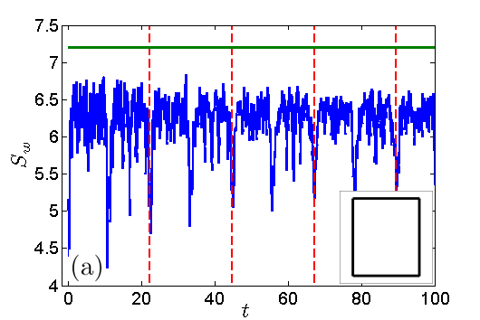
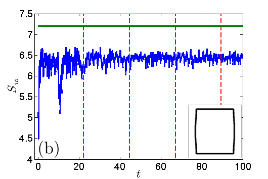
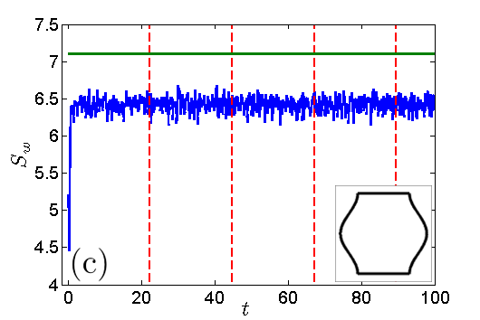
Figure 2: Time evolution of $S_{w}(\psi(t))$ for three different ripple billiards. The initial state is a moving Gaussian wave packet. The dashed red lines indicate the theoretical recurrence time for a square infinite potential well of size $2b\times 2b$. The green lines are the ensemble entropy $S_{E}$. The three ripple billiards shown in the insets are characterized by $\epsilon=a/b=0.25\%,2.5\%,25\%$, respectively.

As we are able to compute the Wannier functions ${\mathit{w}_{j}}$ numerically, the entropy for quantum pure states and the relaxation of our entropy towards a maximum can now be illustrated with a concrete example. We are trying to answer whether a macroscopic many-body quantum system can equilibrate dynamically. However, as we have seen in this work and in many others’ workvon Neumann (1929); Reimann (2008), the conclusion relies on only the structure of eigen-energies of the system (degeneracy, energy gaps, etc.), which are shared by both single-particle and many-body systems according to the random matrix theoryStöckmann (1999). This means that in many situations it is sufficient to use single-particle systems to illustrate entropy for pure states and the quantum H-theorem.

We choose to use ripple billiard with which we are very familiar. The ripple billiard is an infinite potential well with $V=0$ in the area enclosed by $y=\pm b$, $x=\pm b\pm a\cos(\pi y/b)$ and $V=\infty$ otherwiseLi et al. (2002); Xiong and Wu (2011). In our numerical computation, the initial state is a moving Gaussian wave packet and the simulation is carried out on a $64\times 64$ grid. The results for the entropy $S_{w}(\psi(t))$ are plotted in Fig. 2 for ripple billiards with three different values of $\epsilon=a/b$. When $\epsilon$ is small, the system is nearly integrable and $S_{w}$ is almost periodic but with a decaying oscillating amplitude (see Fig. 2(a)). As $\epsilon$ becomes larger and the system gets far away from the integrable regime, the entropy $S_{w}$ rises quickly to a maximum value and stays there with small fluctuations as discussed. The ensemble entropy $S_{E}$ is also plotted and it deviates visibly from the long-time averaged value of $S_{w}$. The reason is that since this is a single-particle system, $S_{w}$ and $S_{E}$ are not large. As a result, the right-hand side of the inequality (22) is not very small.

A few remarks are warranted before we conclude this section. There seems to be a hidden assumption in von Neumann’s proof of his quantum H-theorm besides two explicitly-stated conditions (identical to conditions 1 and 2 here). This assumption is equivalent to eigenstate thermalization hypothesis Srednicki (1994); Rigol et al. (2008) as pointed out in Ref.Rigol and Srednicki (2012) and by an anonymous referee. In our opinion, this assumption is linked directly to Eq.(27) in von Neumann’s proof Neumann (2010), which is highly questionable. In contrast, we do not have any other assumption in our proof of the inequality Eq. (22) besides the three conditions. The conditions for $C$ to be small, such as the hierarchy of energy scales, have also been explicitly expressed. Our effort here is to follow the line of von Neumann and Reimann to understand the microscopic origin of the second law of thermodynamics without any hypothesis. It is true that our inequality with $C\approx 0$ does not exclude the happening of large deviation from the maximized entropy. However, this kind of large deviation occurs rarely according to our analysis. More efforts are needed to find out exactly how rare these events are. The usual fluctuation theorem seems not applicable here as it depends on many concepts, such as temperature, heat bath, and entropy, whose quantum origins are not clear themselves.

V Generalization to mixed states and comparison with von Neumann’s entropy

In quantum mechanics, we are all familiar with the von Neumann entropy that is defined as

$$S_{v}(\rho)\equiv-\mathrm{tr}\;\rho\ln\rho\,,$$ (29)

where $\rho$ is the density matrix for mixed states. This entropy $S_{v}$ is zero for any pure state. This fact leads to a well-known dilemma: a large system in a pure state has zero entropy while any of its subsystems that interacts or entangles with the rest of the system has non-zero entropy $S_{v}$.

To compare our entropies to $S_{v}$, we need to generalize our entropy for mixed states. There is a straightforward way to accomplish the goal: for $N$-particle mixed states $\rho^{N}$, we define

$$S_{w}(\rho^{N})\equiv\sum_{j_{1}j_{2}\dots j_{N}}s_{w}(\,\mathrm{tr}\,\rho^{N}\bm{W}_{j_{1}}\otimes\bm{W}_{j_{2}}\otimes\cdots\otimes\bm{W}_{j_{N}})$$ (30)

where $s_{w}(\wp)=-\wp\ln\wp$.

Several basic properties that $S_{w}(\rho^{N})$ shares with $S_{v}$ Wehrl (1978) are listed below :

Invariance

$S_{w}(\rho^{N})$ depends on $\{w_{j}\}$ but not on the choice of basis in the Hilbert space. This is a result of the invariance of the trace.

Positivity

$S_{w}\geq 0$ since $s_{w}(x)\geq 0$ for $0\leq x\leq 1$.

Concavity

For $\lambda_{1},\lambda_{2}>0$, $\lambda_{1}+\lambda_{2}=1$,

$$S_{w}(\lambda_{1}\rho_{1}^{N}+\lambda_{2}\rho_{2}^{N})\geq\lambda_{1}S_{w}(\rho_{1}^{N})+\lambda_{2}S_{w}(\rho_{2}^{N}).$$ (31)

This originates from the concavity of $s_{w}(x)$.

Additivity

$$S_{w}(\rho_{1}^{M}\otimes\rho_{2}^{N})=S_{w}(\rho_{1}^{M})+S_{w}(\rho_{2}^{N})$$ (32)

The equality indicates that for two independent systems, the total entropy is the sum of the two. The property is also inherited from $s_{w}(x)$.

Proof of these properties is essentially the same as that in Wehrl (1978) and hence omitted here.

Despite these similarities, there is one crucial difference between our entropy and $S_{v}$. As we have mentioned, for $S_{v}$ there is a well-known dilemma: for a large system on a pure state, $S_{v}=0$ while its subsystem has non-zero entropy. In stark contrast, as we shall show, for our entropy $S_{w}$, a large system always has bigger entropy than its subsystem. To demonstrate this, we only need to prove that the entropy $S_{w}$ decreases when one particle is traced out of an $N$-particle system.

Without loss of generality, we tend to trace out the $N^{\textrm{th}}$ particle and write

$$\rho^{N}=\sum_{i,i_{N},i^{\prime},i^{\prime}_{N}}c_{i,i_{N},i^{\prime},i^{\prime}_{N}}|\psi_{i}^{N-1},\psi_{i_{N}}\rangle\langle\psi_{i^{\prime}}^{N-1},\psi_{i^{\prime}_{N}}|\,.$$ (33)

Here $\psi$’s are general orthonormal basis, not energy eigenstates. With the use of the inequality $s_{w}(\wp_{1}+\wp_{2})\leq s_{w}(\wp_{1})+s_{w}(\wp_{2})$ for $\wp_{1},\wp_{2}\geq 0$, the proof is straightforward.

$$S_{w}(\rho^{N})$$

$$=\sum_{j,j_{N}}s_{w}(\sum c\langle\psi_{i^{\prime}}^{N-1}|\bm{W}_{j}^{N-1}|\psi_{i}^{N-1}\rangle\langle\psi_{i^{\prime}_{N}}|\bm{W}_{j_{N}}|\psi_{i_{N}}\rangle)$$

$$\geq\sum_{j}s_{w}(\sum_{j_{N}}\sum c\langle\psi_{i^{\prime}}^{N-1}|\bm{W}_{j}^{N-1}|\psi_{i}^{N-1}\rangle\langle\psi_{i^{\prime}_{N}}|\bm{W}_{j_{N}}|\psi_{i_{N}}\rangle)$$

$$=\sum_{j}s_{w}(\sum c\langle\psi_{i^{\prime}}^{N-1}|\bm{W}_{j}^{N-1}|\psi_{i}^{N-1}\rangle\langle\psi_{i^{\prime}_{N}}|\sum_{j_{N}}\bm{W}_{j_{N}}|\psi_{i_{N}}\rangle)$$

$$=\sum_{j}s_{w}(\sum c\langle\psi_{i^{\prime}}^{N-1}|\bm{W}_{j}^{N-1}|\psi_{i}^{N-1}\rangle\langle\psi_{i^{\prime}_{N}}|\psi_{i_{N}}\rangle)$$

$$=S_{w}(\rho^{N-1})$$ (34)

where the subscripts $i,i_{N},i^{\prime},i^{\prime}_{N}$ are omitted for brevity without causing confusion.

We introduce a density matrix

$$\rho_{\rm mc}=\sum_{\alpha}|\braket{\psi(0)}{\phi_{\alpha}}|^{2}\ket{\phi_{\alpha}}\bra{\phi_{\alpha}}\,.$$ (35)

This density matrix can be regarded as a micro-canonical ensemble for two reasons: (1) It is easy to check that $S_{E}=S_{w}(\rho_{\rm mc})$. This means that the system’s entropy is essentially given by $\rho_{\rm mc}$ at equilibrium. (2) Reimann Reimann (2008) has also shown that the expectation of all observables can be also be computed with $\rho_{\rm mc}$ at equilibrium. This ensemble is clearly different from the conventional micro-canonical ensemble in textbooks Huang (1987) as it depends on the initial condition. The ensemble in Eq. (35) is also different from von Neumann’svon Neumann (1929) that involves certain coarse-graining of energy. However, both our ensemble and von Neumann’s depend more or less on the choice of initial conditions. This can lead to very interesting new physics: we are at liberty to choose an initial condition that composes of energy-eigenstates from two very different energy shells, which can lead to an equilibrium state with two distinct temperaturesZhuang and Wu (2014).

VI Conclusion

In summary, we have used Kohn’s method to construct a complete set of Wannier functions which are localized at both given positions and momenta. We then established a quantum phase space, where each Planck cell is represented by one of these Wannier functions. By mapping unitarily a quantum pure state to this quantum phase space, we have defined an entropy for pure states. A hierarchy of energy scales is proposed and the properties of this entropy have been examined. In particular, we have shown that for our entropy, a system always has larger entropy than its subsystems.

The long-time dynamical behavior of our entropy has been examined and found to obey an inequality, which like the quantum H-theorem proved by von Neumannvon Neumann (1929), along with reasonable hypotheses, indicates that majority of isolated quantum systems equilibrate dynamically: starting with reasonable initial states, the quantum system will evolve into a state with maximized entropy and stay there almost all the time with small fluctuations. Due to the time reversal symmetry, the system does sometimes undertake large fluctuations. However, the quantum H-theorem demands that these large fluctuations happen rarely and are short-lived, which provides a quantum perspective of the second law of thermodynamics.

As already pointed out in the introduction, there have been renewed interests in the foundation of quantum statistical mechanics. These new efforts have not only led to better theoretical understanding of the issue but also to new physical predications and challenges that await for answers from experimentalists. For example, a quantum state which is at equilibrium but with multiple temperatures was predicted based on the micro-cannonical ensemble established by von NeumannZhuang and Wu (2014). And it was shown recentlyGoldstein et al. (2014); Monnai (2014); Malabarba et al. (2014) that quantum systems can relax much faster than what has been observed in reality. Can this multiple temperature state be realized in experiments? Does it really exist a quantum state that can relax as fast as what the theorists have predicted? The answers may ultimately lie in understanding the borderline between the microscopic and the macroscopic world.

VII Acknowledgments

We thank Hongwei Xiong and Michael Kastner for helpful discussion. This work is supported by the NBRP of China (2013CB921903,2012CB921300) and the NSF of China (11274024,11334001).

Appendix A Proposition for orthogonalization

We prove here a proposition based on which one can show the orthogonality of $\{w_{j}(x)\}$.

Proposition 1.

Assume $f_{j}(k)\in L^{2}(\mathbb{R})$ ($j\in\mathbb{N}$) if for almost every $k\in[0,2\pi)$, for all $j,j^{\prime}\in\mathbb{N}$

$$\sum_{n\in\mathbb{Z}}f_{j}^{*}(k+2n\pi)f_{j^{\prime}}(k+2n\pi)=\frac{1}{2\pi}\delta_{jj^{\prime}}\,,$$ (36)

then we have

$$\int_{\mathbb{R}}f_{j}^{*}(k)f_{j^{\prime}}(k)\mathrm{e}^{-ij_{x}k}\;\mathrm{d}k=\delta_{jj^{\prime}}\delta_{0j_{x}}$$ (37)

for all $j,j^{\prime}\in\mathbb{N}$ and $j_{x}\in\mathbb{Z}$.

Proof.

$$\int_{\mathbb{R}} f_{j}^{*}(k)f_{j^{\prime}}(k)\mathrm{e}^{-ij_{x}k}\;\mathrm{d}k$$

$$=\sum_{n\in\mathbb{Z}}\int_{2n\pi}^{2(n+1)\pi}f_{j}^{*}(k)f_{j^{\prime}}(k)\mathrm{e}^{-ij_{x}k}\;\mathrm{d}k$$

$$=\sum_{n\in\mathbb{Z}}\int_{0}^{2\pi}f_{j}^{*}(k+2n\pi)f_{j^{\prime}}(k+2n\pi)\mathrm{e}^{-ij_{x}(k+2n\pi)}\;\mathrm{d}k$$

$$=\int_{0}^{2\pi}\sum_{n\in\mathbb{Z}}f_{j}^{*}(k+2n\pi)f_{j^{\prime}}(k+2n\pi)\mathrm{e}^{-ij_{x}k}\;\mathrm{d}k$$

$$=\frac{\delta_{jj^{\prime}}}{2\pi}\int_{0}^{2\pi}\mathrm{e}^{-ij_{x}k}\;\mathrm{d}k=\delta_{jj^{\prime}}\delta_{0j_{x}}$$

∎

The converse is also valid and the proof is omitted here. For the construction of localized orthonormal basis in the main text, $f_{j}(k)=\tilde{\mathit{w}}_{j_{k}}(k)$. Noticing that

$$\int_{\mathbb{R}}\mathcal{F}\{f(x)\}^{*}(k)\mathcal{F}\{g(x)\}(k)\;\mathrm{d}k=\int_{\mathbb{R}}f^{*}(x)g(x)\;\mathrm{d}x$$ (38)

and $\mathcal{F}\{f(x-j_{x})\}=\mathcal{F}\{f(x)\}\mathrm{e}^{-ij_{x}k}$, where

$$\mathcal{F}\{f(x)\}(k)\equiv\frac{1}{\sqrt{2\pi}}\int_{\mathbb{R}}f(x)\mathrm{e}^{-ikx}\;\mathrm{d}x\,,$$ (39)

we have

$$\int_{\mathbb{R}}\mathit{w}_{j_{k}}^{*}(x)\mathit{w}_{j^{\prime}_{k}}(x-j_{x})\;\mathrm{d}x$$ (40)

$$= \int_{\mathbb{R}}\mathcal{F}\{\mathit{w}_{j_{k}}(x)\}^{*}(k)\mathcal{F}\{\mathit{w}_{j^{\prime}_{k}}(x-j_{x})\}(k)\;\mathrm{d}k$$

$$= \int_{\mathbb{R}}\tilde{\mathit{w}}_{j_{k}}^{*}(k)\tilde{\mathit{w}}_{j^{\prime}_{k}}(k)\mathrm{e}^{-ij_{x}k}\;\mathrm{d}k=\delta_{j_{k}j^{\prime}_{k}}\delta_{0j_{x}}\,.$$

Appendix B Strong uncertainty relation

The numerical results in main text with Gaussian wave packets as the initial non-orthogonal basis indicate that $\Delta x_{j}\cdot\Delta k_{j}$ diverge at large $k$. In fact this divergence does not depend on the choice of initial wave packets; it is always the case as long as one uses Kohn’s method to generate a complete set of basis that has translational symmetry. Here we offer the proof.

Let $\{\mathit{w}_{j_{k}}(x-j_{x})\}_{j_{k},j_{x}\in\mathbb{Z}}$ be an orthonormal basis generated from initial wave packets $\tilde{g}_{j_{k}}$ as discussed in section II. For convenience, we apply Schidmit orthogonalization process in order $j_{k}=0,1,-1,2,-2,\dots$ First we show that $h(k)\equiv\lim_{j_{k}\rightarrow+\infty}\tilde{w}_{j_{k}}(k+2j_{k}\pi)$ exists. Since $\tilde{\mathit{w}}_{j_{k}}(k+2n\pi)\equiv v_{k,j_{k}}(n)/\sqrt{2\pi}$, it is sufficient to prove that for any fixed $k$, $v_{k}(n)\equiv\lim_{j_{k}\to+\infty}v_{k,j_{k}}(n+j_{k})$ exists. Introduce a subspace of $l^{2}(\mathbb{Z})$

$$H_{k,l}\equiv\mathop{\mathrm{span}}_{|j_{k}|\leq l}v_{k,j_{k}}(n+l+1)$$ (41)

for $l\in\mathbb{N}$. Noticing $v_{k,j_{k}}$ is the linear combination of $u_{k,j^{\prime}_{k}}$ ($|j^{\prime}_{k}|\leq|j_{k}|$),

$$H_{k,l} =\mathop{\mathrm{span}}_{|j_{k}|\leq l}u_{k,j_{k}}(n+l+1)$$ (42)

$$=\mathop{\mathrm{span}}_{|j_{k}|\leq l}\tilde{g}_{j_{k}}(k+2(n+l+1)\pi)$$

$$=\mathop{\mathrm{span}}_{|j_{k}|\leq l}\tilde{g}_{0}(k+2(n+l-j_{k}+1)\pi)$$

$$=\mathop{\mathrm{span}}_{1\leq j_{k}\leq 2l+1}\tilde{g}_{0}(k+2j_{k}\pi+2n\pi)$$

From Schidmit orthogonalization process, we know that

$$v_{k,l+1}(n+l+1) =\bm{N}\bm{P}_{H_{k,l}^{\bot}}u_{k,l+1}(n+l+1)$$ (43)

$$=\bm{N}\bm{P}_{H_{k,l}^{\bot}}\tilde{g}_{0}(k+2n\pi)$$

where $\bm{N}$ is the normalization operator and $\bm{P}$ is the projection operator. We have to prove that as $l\to+\infty$, the limit of (43) exists. Since $\bm{N}$ is continuous except at the origin, it is sufficient to show that

$$\lim_{l\to+\infty}\bm{P}_{H_{k,l}^{\bot}}\tilde{g}_{0}(k+2n\pi)\;\textrm{exists and}\;\neq 0.$$ (44)

Denote $r_{k,l}\equiv\bm{P}_{H_{k,l}^{\bot}}\tilde{g}_{0}(k+2n\pi)$. Since $H_{k,l}^{\bot}$ is monotonically decreasing and $\bm{P}$ is orthogonal projection, $\|r_{l}\|$(subscript $k$ omitted) is decreasing and $r_{l}-r_{l^{\prime}}\bot r_{l^{\prime}}$ for $l<l^{\prime}$. Hence $\|r_{l}-r_{l^{\prime}}\|^{2}=\|r_{l}\|^{2}-\|r_{l^{\prime}}\|^{2}\to 0$ as $l\to+\infty$. $\{r_{l}\}$ converges.

Note that

$$r_{k}\equiv\lim_{l\to+\infty}r_{k,l}\neq 0\Leftrightarrow\tilde{g}_{0}(k+2n\pi)\notin H_{k}\equiv\overline{\bigcup_{l\in\mathbb{N}}H_{k,l}}.$$ (45)

For reasonable initial wave packets, this is always the case. For example, when $\tilde{g}_{0}$ is compactly supported, $\exists N$ such that $\tilde{g}_{0}(k+2N\pi)\neq 0$ and $\forall n>N$, $\tilde{g}_{0}(k+2n\pi)=0$, hence $\tilde{g}_{0}\notin H_{k}$.

From the proof above, we see $v_{k,l+1}\in H_{k,l}^{\bot}$, hence, $v_{k,l+1}\bot v_{k,j_{k}}$ for all $|j_{k}|\leq l$. As a result of the limiting process, $r_{k}(n)\bot r_{k}(n+p)$ for all $p\neq 0$. The proof is valid for every $k$, hence $h(k)$ and its translations form a periodic orthonormal basis. Due to Balian’s proofBourgain (1988), for $h$, $\Delta x=\infty$ or $\Delta k=\infty$. Thus, no matter how the initial wave packet is chosen, by our orthogonalization approach, strong uncertainty relation holds, if space translational symmetry is required, i.e.

$$\sup\Delta x_{j}\sup\Delta k_{j}=\infty.$$

Appendix C Proof of the inequality

Here we present the detailed proof of the inequality (22). First we provide two inequalities that will be useful later:

$$\overline{\left(\wp_{j}(t)-\overline{\wp}_{j}\right)^{2}}\leq\overline{\wp}_{j}^{2}\,,$$ (46)

and

$$\overline{\left(\wp_{j}(t)-\overline{\wp}_{j}\right)^{4}}\leq 9\overline{\wp}_{j}^{4}\,.$$ (47)

Derivation of inequality (46) needs conditions 1 and 2 while for inequality (47) all three conditions are necessary. The proof of the inequality (46) is as follows.

$$\overline{\left(\wp_{j}(t)-\overline{\wp_{j}}\right)^{2}} =\sum_{\alpha\neq\beta}c_{\alpha j}c_{\alpha j}^{*}c_{\beta j}c_{\beta j}^{*}$$

$$=\overline{\wp}_{j}^{2}-\sum_{\alpha}|c_{\alpha j}|^{4}\leq\overline{\wp}_{j}^{2}\,.$$ (48)

It is straightforward but more care is needed to prove (47). Since in the proof, only one Planck cell $j$ is considered, we suppress the subscript $j$ of $c_{\alpha j}$ for brevity. Before time averaging, we have

$$\left(\wp_{j}(t)-\overline{\wp}_{j}\right)^{4}=\big{(}\sum_{\alpha\neq\alpha^{\prime}}c_{\alpha}c_{\alpha^{\prime}}^{*}\mathrm{e}^{i(E_{\alpha}-E_{\alpha^{\prime}})t}\big{)}^{4}$$ (49)

$$= \sum_{\alpha\neq\alpha^{\prime},\beta\neq\beta^{\prime}}^{\chi\neq\chi^{\prime},\gamma\neq\gamma^{\prime}}c_{\alpha}c_{\alpha^{\prime}}^{*}c_{\beta}c_{\beta^{\prime}}^{*}c_{\chi}^{*}c_{\chi^{\prime}}c_{\gamma}^{*}c_{\gamma^{\prime}}$$

$$\times~{}\mathrm{e}^{i(E_{\alpha}+E_{\beta}+E_{\chi^{\prime}}+E_{\gamma^{\prime}}-E_{\alpha^{\prime}}-E_{\beta^{\prime}}-E_{\chi}-E_{\gamma})t}\,.$$

This yields

$$\overline{\left(\wp_{j}(t)-\overline{\wp}_{j}\right)^{4}}=$$

$$\overline{\sum}_{\alpha\neq\alpha^{\prime},\beta\neq\beta^{\prime}}^{\chi\neq\chi^{\prime},\gamma\neq\gamma^{\prime}}c_{\alpha}c_{\alpha^{\prime}}^{*}c_{\beta}c_{\beta^{\prime}}^{*}c_{\chi}^{*}c_{\chi^{\prime}}c_{\gamma}^{*}c_{\gamma^{\prime}}\,,$$ (50)

where the overlined summation is over only the terms that satisfy the energy relation

$$E_{\alpha^{\prime}}+E_{\beta^{\prime}}+E_{\chi}+E_{\gamma}=E_{\alpha}+E_{\beta}+E_{\chi^{\prime}}+E_{\gamma^{\prime}}\,.$$ (51)

This sum can be divided into four parts.

• $\alpha=\beta^{\prime}$ and $\beta=\alpha^{\prime}$ .
  In this case, the energy relation becomes $E_{\chi}+E_{\gamma}=E_{\chi^{\prime}}+E_{\gamma^{\prime}}$. According to condition 2, $\chi=\gamma^{\prime}$ and $\gamma=\chi^{\prime}$. The sum of relevant terms converts into

  $$\sum_{\alpha\neq\beta,\chi\neq\gamma}c_{\alpha}c_{\beta}^{*}c_{\beta}c_{\alpha}^{*}c_{\chi}^{*}c_{\gamma}c_{\gamma}^{*}c_{\chi}\leq\overline{\wp}_{j}^{4}\,.$$ (52)

• $\alpha=\beta^{\prime}$ and $\beta\neq\alpha^{\prime}$  .
  The energy relation is now

  $$E_{\chi}+E_{\gamma}-E_{\beta}=E_{\chi^{\prime}}+E_{\gamma^{\prime}}-E_{\alpha^{\prime}}\,.$$ (53)

  (i) When $\chi=\beta$, $E_{\gamma}-E_{\gamma^{\prime}}=E_{\chi^{\prime}}-E_{\alpha^{\prime}}$. With condition 2, this implies that $\gamma=\chi^{\prime}$ and $\gamma^{\prime}=\alpha^{\prime}$. We then have

  $$\sum_{\alpha\neq\alpha^{\prime},\beta\neq\alpha}^{\beta\neq\gamma,\gamma\neq\alpha^{\prime}}c_{\alpha}c_{\alpha^{\prime}}^{*}c_{\beta}c_{\alpha}^{*}c_{\beta}^{*}c_{\gamma}c_{\gamma}^{*}c_{\alpha^{\prime}}\leq\overline{\wp}_{j}^{4}\,.$$ (54)

  (ii) When $\chi\neq\beta$, we have $\gamma=\beta$. This can be seen in the energy relation $E_{\chi}+E_{\gamma}-E_{\beta}-E_{\delta}=E_{\chi^{\prime}}+E_{\gamma^{\prime}}-E_{\alpha^{\prime}}-E_{\delta}$ with $E_{\delta}$ being an arbitrary eigen-energy. If $\gamma\neq\beta$, choose $\delta$ such that $\{\chi,\gamma\}\cap\{\beta,\delta\}=\emptyset$; according to condition 3, it is required $\beta=\alpha^{\prime}$ which is a contradiction. Since $\gamma=\beta$, the rest calculation is similar to that in (i).

  Overall, this part of summation is no more than $2\overline{\wp}_{j}^{4}$.

• $\alpha\neq\beta^{\prime}$ and $\beta=\alpha^{\prime}$ .
  Similarly, this part contributes $2\overline{\wp}_{j}^{4}$.

• $\{\alpha,\beta\}\cap\{\alpha^{\prime},\beta^{\prime}\}=\emptyset$ .
  In this case, condition 3 demands that $\{\alpha,\beta\}=\{\chi,\gamma\}$ and $\{\alpha^{\prime},\beta^{\prime}\}=\{\chi^{\prime},\gamma^{\prime}\}$. Among the four different combinations, we choose $\alpha=\chi,\beta=\gamma,\alpha^{\prime}=\gamma^{\prime},\beta^{\prime}=\chi^{\prime}$, which leads to

  $$\sum_{\alpha\neq\alpha^{\prime},\gamma\neq\beta^{\prime}}^{\gamma\neq\alpha^{\prime}}c_{\alpha}c_{\alpha^{\prime}}^{*}c_{\gamma}c_{\beta^{\prime}}^{*}c_{\alpha}^{*}c_{\beta^{\prime}}c_{\gamma}^{*}c_{\alpha^{\prime}}\leq\overline{\wp}_{j}^{4}\,.$$ (55)

  As the three other combinations are similar, the sum is less or equal to $4\overline{\wp}_{j}^{4}$.

Summing all these cases, we obtain the inequality (47).

In the proof, we also use the following equality: for $\wp,\overline{\wp}\geq 0$, there exists $0<\xi\leq 1$ such that

$$\wp\ln\wp=\overline{\wp}\ln\overline{\wp}+(1+\ln\overline{\wp})(\wp-\overline{\wp})+\frac{\xi(\wp-\overline{\wp})^{2}}{\overline{\wp}}\,.$$ (56)

We are now ready to present the full proof of the inequality (22). Assume for every $j$, $\overline{\wp}_{j}<1/\mathrm{e}$.

$$\overline{\left(\sum_{j}\left[\wp_{j}(t)\ln\wp_{j}(t)-\overline{\wp}_{j}\ln\overline{\wp}_{j}\right]\right)^{2}}=\overline{\left(\sum_{j}\left[(1+\ln\overline{\wp}_{j})(\wp_{j}(t)-\overline{\wp}_{j})+\frac{\xi_{j}(t)(\wp_{j}(t)-\overline{\wp}_{j})^{2}}{\overline{\wp}_{j}}\right]\right)^{2}}$$

$$= \sum_{j,j^{\prime}}(1+\ln\overline{\wp}_{j})(1+\ln\overline{\wp}_{j^{\prime}})\overline{(\wp_{j}(t)-\overline{\wp}_{j})(\wp_{j^{\prime}}(t)-\overline{\wp}_{j^{\prime}})}+2\sum_{j,j^{\prime}}\frac{1+\ln\overline{\wp}_{j}}{\overline{\wp}_{j^{\prime}}}\overline{(\wp_{j}(t)-\overline{\wp}_{j})\xi_{j^{\prime}}(t)(\wp_{j^{\prime}}(t)-\overline{\wp}_{j^{\prime}})^{2}}$$

$$\quad+\sum_{j,j^{\prime}}\frac{1}{\overline{\wp}_{j}\;\overline{\wp}_{j^{\prime}}}\overline{\xi_{j}(t)\xi_{j^{\prime}}(t)(\wp_{j}(t)-\overline{\wp}_{j})^{2}(\wp_{j^{\prime}}(t)-\overline{\wp}_{j^{\prime}})^{2}}$$

$$\leq \sum_{j,j^{\prime}}(1+\ln\overline{\wp}_{j})(1+\ln\overline{\wp}_{j^{\prime}})\overline{\wp}_{j}\;\overline{\wp}_{j^{\prime}}C_{jj^{\prime}}-2\sum_{j,j^{\prime}}\frac{1+\ln\overline{\wp}_{j}}{\overline{\wp}_{j^{\prime}}}\sqrt{\overline{(\wp_{j}(t)-\overline{\wp}_{j})^{2}}\;\overline{(\wp_{j^{\prime}}(t)-\overline{\wp}_{j^{\prime}})^{4}}}$$

$$\quad+\sum_{j,j^{\prime}}\frac{1}{\overline{\wp}_{j}\;\overline{\wp}_{j^{\prime}}}\sqrt{\overline{(\wp_{j}(t)-\overline{\wp}_{j})^{4}}\;\overline{(\wp_{j^{\prime}}(t)-\overline{\wp}_{j^{\prime}})^{4}}}$$

$$\leq \sum_{j,j^{\prime}}(1+\ln\overline{\wp}_{j})(1+\ln\overline{\wp}_{j^{\prime}})\overline{\wp}_{j}\;\overline{\wp}_{j^{\prime}}C_{jj^{\prime}}-2\sum_{j,j^{\prime}}\frac{1+\ln\overline{\wp}_{j}}{\overline{\wp}_{j^{\prime}}}\overline{\wp}_{j}\;3\overline{\wp}_{j^{\prime}}^{2}+\sum_{j,j^{\prime}}\frac{9}{\overline{\wp}_{j}\;\overline{\wp}_{j^{\prime}}}\overline{\wp}_{j}^{2}\overline{\wp}_{j^{\prime}}^{2}$$

$$\leq CS_{E}^{2}+8S_{E}+4\,.$$

For the first inequality “$\leq$”, we have used $\overline{\wp}_{j}<1/\mathrm{e}$; in the last step, we have used $|C_{jj^{\prime}}|\leq 1$. For a typical wave function of a many-body quantum system, it spreads out over thousands of Planck cells in the phase space; therefore $\overline{\wp}_{j}<1/\mathrm{e}$ is satisfied almost always.

Appendix D Estimate of $S_{E}$ and $C$

Estimate of $S_{E}$

This is equivalent to show Eq. (26).

Suppose that $J\equiv[E,E+\Delta E]$ ($\Delta_{\textrm{C}}E\ll\Delta E\lesssim\Delta_{\textrm{mc}}E$) is a macroscopic energy shell which is significantly occupied by the quantum state $\psi$. For brevity, we use $j\in J$ to represent $E_{j}=\braket{w_{j}}{H}{w_{j}}\in[E,E+\Delta E]$, and $\alpha\in J$ for $E_{\alpha}\in[E,E+\Delta E]$.

As $\Delta_{\textrm{C}}E$ is the correlation energy scale, we have

$$\wp_{\alpha}|\braket{w_{j}}{\phi_{\alpha}}|^{2}\ll 1\,,$$ (57)

when $|E_{j}-E_{\alpha}|\gg\Delta_{\textrm{C}}E$. Since $\Delta E\gg\Delta_{\textrm{C}}E$, we have for a typical (energy away from end points of $J$) $j\in J$

$$\overline{\wp}_{j}\approx\sum_{\alpha\in J}\wp_{\alpha}|\langle w_{j}|\phi_{\alpha}\rangle|^{2}\,,$$ (58)

and for a typical $\alpha\in J$

$$\sum_{j\in J}|\langle w_{j}|\phi_{\alpha}\rangle|^{2}\approx 1\,.$$ (59)

With (17) and (18), these lead to

$$\sum_{j\in J}\overline{\wp}_{j}\approx\sum_{j\in J}\sum_{\alpha\in J}\wp_{\alpha}|\langle w_{j}|\phi_{\alpha}\rangle|^{2}\approx\sum_{\alpha\in J}\wp_{\alpha}\,.$$ (60)

For matrix $A_{j\alpha}\equiv|\langle w_{j}|\phi_{\alpha}\rangle|^{2}$($j\in J$, $\alpha\in J$), the sum of every row of $A^{T}A$ is less than one. By the Perron-Frobenius theorem, the eigenvalue of $A^{T}A$ must be equal or less than one in module and we have

$$\sum_{j\in J}\overline{\wp}_{j}^{2}\approx P^{T}A^{T}AP\leq P^{T}P=\sum_{\alpha\in J}\wp_{\alpha}^{2}\,,$$ (61)

where the column vector $(P)_{\alpha}=\wp_{\alpha}$. We are now ready to estimate the entropy,

$$S_{E,J} \equiv -\sum_{j\in J}\overline{\wp}_{j}\ln\overline{\wp}_{j}\geq-\sum_{j\in J}\overline{\wp}_{j}\ln\big{(}\sum_{j\in J}\overline{\wp}_{j}^{2}\big{/}\sum_{j\in J}\overline{\wp}_{j}\big{)}$$ (62)

$$\gtrsim -\sum_{\alpha\in J}\wp_{\alpha}\ln\big{(}\sum_{\alpha\in J}\wp_{\alpha}^{2}\big{/}\sum_{\alpha\in J}\wp_{\alpha}\big{)}$$

$$\approx -\sum_{\alpha\in J}\wp_{\alpha}\ln\big{(}\langle\wp_{\alpha}\rangle_{s}/R\big{)}$$

$$\approx S_{E,J}^{\max}+\sum_{\alpha\in J}\wp_{\alpha}\ln R\,.\quad$$

In the first line of the above derivation, Jensen’s inequality for function $-\ln x$ is applied. If $J$ is the only energy shell significantly occupied by $\psi$, we already have Eq. (26). If we have more than one such energy shells, we sum Eq. (62) for all $J$ and obtain Eq. (26).

Estimate of $C$

Define $d_{\epsilon,j}$ as the minimal $d$ such that

$$\sum_{|E_{\alpha}-E_{j}|<d}\wp_{\alpha}|\langle w_{j}|\phi_{\alpha}\rangle|^{2}>(1-\epsilon)\overline{\wp}_{j}\,,$$ (63)

where $E_{j}$ is the average energy of $w_{j}$. We say that Planck cells $j$ and $j^{\prime}$ overlap if $|E_{j}-E_{j^{\prime}}|<d_{\epsilon,j}+d_{\epsilon,j^{\prime}}$. We consider two cells $j$ and $j^{\prime}$ which do not overlap. With condition 1 and 2, we have

$$C_{jj^{\prime}}\overline{\wp}_{j}\overline{\wp}_{j^{\prime}}\leq\big{|}\sum_{\alpha}\wp_{\alpha}\langle w_{j}|\phi_{\alpha}\rangle\langle\phi_{\alpha}|w_{j^{\prime}}\rangle\big{|}^{2}\,.$$ (64)

Without loss of generality, we assume $E_{j}<E_{j^{\prime}}$ and split the above sum into two parts: one part close to $j$ and the other close to $j^{\prime}$.

$$C_{jj^{\prime}}\overline{\wp}_{j}\overline{\wp}_{j^{\prime}}\leq 2\big{|}\sum_{E_{\alpha}<E^{\prime}}\wp_{\alpha}\langle w_{j}|\phi_{\alpha}\rangle\langle\phi_{\alpha}|w_{j^{\prime}}\rangle\big{|}^{2}$$

$$+2\big{|}\sum_{E_{\alpha}\geq E^{\prime}}\wp_{\alpha}\langle w_{j}|\phi_{\alpha}\rangle\langle\phi_{\alpha}|w_{j^{\prime}}\rangle\big{|}^{2}\,,$$ (65)

where $E^{\prime}\equiv E_{j}+d_{\epsilon,j}$. The first term, by Cauchy-Schwartz inequality, is less or equal to

$$2\sum_{E_{\alpha}<E^{\prime}}\wp_{\alpha}|\langle w_{j}|\phi_{\alpha}\rangle|^{2}\sum_{E_{\alpha}<E^{\prime}}\wp_{\alpha}|\langle\phi_{\alpha}|w_{j^{\prime}}\rangle|^{2}<2\epsilon\;\overline{\wp}_{j}\overline{\wp}_{j^{\prime}}\,.$$ (66)

Similar argument applies to the second term and we have

$$C_{jj^{\prime}}\leq 4\epsilon\,.$$ (67)

Next we need to establish that non-overlapping Planck cells are the majority in the pair of cells involved. For this purpose, it is sufficient to show that for any significantly occupied Planck cell $j$, the sum $S_{j}$ of entropies over cells overlapping with $j$ is much less than $S_{E}$. This is indeed the case,

$$S_{j} \lesssim -\int_{E_{j}-d_{\epsilon}}^{E_{j}+d_{\epsilon}}\mathrm{d}E\;\rho(E)\langle\wp_{\alpha}\rangle_{s}(E)\ln\langle\wp_{\alpha}\rangle_{s}(E)\qquad$$ (68)

$$\ll -\int_{E_{j}-\Delta_{\textrm{mc}}E}^{E_{j}+\Delta_{\textrm{mc}}E}\mathrm{d}E\;\rho(E)\langle\wp_{\alpha}\rangle_{s}(E)\ln\langle\wp_{\alpha}\rangle_{s}(E)$$

$$\leq S_{E}^{\max}\approx S_{E}\,.$$

In the above derivation, we have used that $\langle\wp_{\alpha}\rangle$ are effectively constant on a range of $\Delta_{\textrm{mc}}E$, $S_{E}$ is maximized, and assumption (18). This yields the inequality (28) if we set $\epsilon=\Delta_{\textrm{C}}E/\Delta_{\textrm{mc}}E$ and hence $\Delta_{\textrm{C}}E\ll d_{\epsilon}\lesssim\sqrt{\Delta_{\textrm{C}}E\Delta_{\textrm{mc}}E}\ll\Delta_{\textrm{mc}}E$ (estimated according to Eq. (15) and (63) for typical $j$).

References

• Huang (1987) K. Huang, Statistical Mechanics (Wiley, New York, 1987).
• von Neumann (1929) J. von Neumann, Zeitschrift für Physik 57, 30 (1929).
• Goldstein et al. (2010a) S. Goldstein, J. L. Lebowitz, R. Tumulka, and N. Zanghì, The European Physical Journal H 35, 173 (2010a).
• Kinoshita et al. (2006) T. Kinoshita, T. Wenger, and D. S. Weiss, Nature 440, 900 (2006).
• Smith et al. (2013) D. A. Smith, M. Gring, T. Langen, M. Kuhnert, B. Rauer, R. Geiger, T. Kitagawa, I. Mazets, E. Demler, and J. Schmiedmayer, New Journal of Physics 15, 075011 (2013).
• Yukalov (2011a) V. I. Yukalov, Laser Physics Letters 8, 485 (2011a).
• Gemmer et al. (2004) J. Gemmer, M. Michel, and G. Mahler, Quantum thermodynamics, no. 657 in Lecture Notes in Physics (Springer-Verlag, Berlin, 2004).
• Srednicki (1994) M. Srednicki, Phys. Rev. E 50, 888 (1994).
• Goldstein et al. (2006) S. Goldstein, J. L. Lebowitz, R. Tumulka, and N. Zanghì, Phys. Rev. Lett. 96, 050403 (2006).
• Popescu et al. (2006) S. Popescu, A. J. Short, and A. Winter, Nat Phys 2, 754 (2006).
• Dong et al. (2007) H. Dong, S. Yang, X. F. Liu, and C. P. Sun, Phys. Rev. A 76, 044104 (2007).
• Rigol et al. (2008) M. Rigol, V. Dunjko, and M. Olshanii, Nature 452, 854 (2008).
• Goldstein et al. (2010b) S. Goldstein, J. L. Lebowitz, C. Mastrodonato, R. Tumulka, and N. Zanghì, Proceedings of the Royal Society A: Mathematical, Physical and Engineering Science 466, 3203 (2010b).
• Linden et al. (2009) N. Linden, S. Popescu, A. J. Short, and A. Winter, Phys. Rev. E 79, 061103 (2009).
• Reimann (2007) P. Reimann, Phys. Rev. Lett. 99, 160404 (2007).
• Reimann (2008) P. Reimann, Phys. Rev. Lett. 101, 190403 (2008).
• Reimann and Kastner (2012) P. Reimann and M. Kastner, New Journal of Physics 14, 043020 (2012).
• Cho and Kim (2010) J. Cho and M. S. Kim, Phys. Rev. Lett. 104, 170402 (2010).
• Ikeda et al. (2011) T. N. Ikeda, Y. Watanabe, and M. Ueda, Phys. Rev. E 84, 021130 (2011).
• Ji and Fine (2011) K. Ji and B. V. Fine, Physical Review Letters 107, 050401 (2011).
• Yukalov (2011b) V. Yukalov, Physics Letters A 375, 2797 (2011b), ISSN 0375-9601.
• Sugiura and Shimizu (2012) S. Sugiura and A. Shimizu, Phys. Rev. Lett. 108, 240401 (2012).
• Snoke et al. (2012) D. Snoke, G. Liu, and S. Girvin, Annals of Physics 327, 1825 (2012), ISSN 0003-4916, july 2012 Special Issue.
• Wang (2012) W.-g. Wang, Phys. Rev. E 86, 011115 (2012).
• Rigol and Srednicki (2012) M. Rigol and M. Srednicki, Phys. Rev. Lett. 108, 110601 (2012).
• Riera et al. (2012) A. Riera, C. Gogolin, and J. Eisert, Phys. Rev. Lett. 108, 080402 (2012).
• Ududec et al. (2013) C. Ududec, N. Wiebe, and J. Emerson, Phys. Rev. Lett. 111, 080403 (2013).
• Zhuang and Wu (2014) Q. Zhuang and B. Wu, Laser Physics Letters 11, 085501 (2014).
• Goldstein et al. (2014) S. Goldstein, T. Hara, and H. Tasaki, arXiv:1402.0324 (2014).
• Neumann (2010) J. Neumann, The European Physical Journal H 35, 201 (2010), ISSN 2102-6459.
• Goldstein et al. (2010c) S. Goldstein, J. L. Lebowitz, C. Mastrodonato, R. Tumulka, and N. Zanghi, Phys. Rev. E 81, 011109 (2010c).
• Short (2011) A. J. Short, New Journal of Physics 13, 053009 (2011), ISSN 1367-2630.
• Zhuang and Wu (2013) Q. Zhuang and B. Wu, Phys. Rev. E 88, 062147 (2013).
• Kohn (1973) W. Kohn, Phys. Rev. B 7, 4388 (1973).
• Zachos et al. (2005) C. K. Zachos, D. B. Fairlie, and T. L. Curtright, eds., Quantum Mechanics in Phase Space (World Scientific, Singapore, 2005).
• Bourgain (1988) J. Bourgain, Journal of functional analysis 79, 136 (1988).
• Short and Farrelly (2012) A. J. Short and T. C. Farrelly, New Journal of Physics 14, 013063 (2012), ISSN 1367-2630.
• Stöckmann (1999) H.-J. Stöckmann, Quantum Chaos: An Introduction (Cambridge University Press, Cambridge, 1999).
• Li et al. (2002) W. Li, L. E. Reichl, and B. Wu, Phys. Rev. E 65, 056220 (2002).
• Xiong and Wu (2011) H. Xiong and B. Wu, Laser Physics Letters 8, 398 (2011).
• Wehrl (1978) A. Wehrl, Rev. Mod. Phys. 50, 221 (1978).
• Polkovnikov (2011) A. Polkovnikov, Annals of Physics 326, 486 (2011), ISSN 0003-4916.
• Monnai (2014) T. Monnai, J. Phys. Soc. Jpn 83, 064001 (2014).
• Malabarba et al. (2014) A. S. Malabarba, L. P. García-Pintos, N. Linden, T. C. Farrelly, and A. J. Short, arXiv:1402.1093 (2014).