Predictive Capabilities of Avalanche Models for Solar Flares

Abstract

We assess the predictive capabilities of various classes of avalanche models for solar flares. We demonstrate that avalanche models cannot generally be used to predict specific events due to their high sensitivity to their embedded stochastic process. We show that deterministically driven models can nevertheless alleviate this caveat and be efficiently used for large events predictions. Our results promote a new approach for large (typically X-class) solar flares predictions based on simple and computationally inexpensive avalanche models.

1 Introduction

sec:introduction

It has now been clearly established that solar eruptive phenomena have multiple incidences on the heliosphere, and in particular on the Earth space environment. Along with coronal mass ejections (CMEs, see Chen, 2011), solar flares are one of the most dangerous space weather events. They are also systematically observed before a large CME is triggered (Shibata and Magara, 2011). While CME-triggered energetic particles reach Earth on time scales of tens of hours, high energy protons accelerated by a flaring process may reach 1 AU few tens of minutes later, and the associated X-ray photons affecting the Earth’s ionosphere only 8 minutes later. No robust precursor of solar flares have been identified so far, preventing any efficient empirical forecast. An ongoing significant effort to predict when a flare of a given magnitude will occur have been pursued over the last decade (for a recent review, see Georgoulis, 2012, and references therein), with moderate success so far. Any progress in this direction is thus highly valuable for risk management related to space weather.

Decades of flare observations have shown that the probability distribution function $f(E)$ for flare energy $E$ takes the form of a power law, $f(E)\propto E^{-\alpha}$ spanning some 8 orders of magnitude in energy, with estimated in the range $1.4-2.0$ (Aschwanden and Parnell, 2002; Aschwanden, 2011). Avalanches provide one class of physical phenomena characterized by such scale-free energy release when driven slowly and continuously. Many avalanche models have been developed to represent the solar flares distribution (see Charbonneau, 2013, and references therein), most of which are based on the concept of self-organized criticality (hereafter SOC; see Bak, Tang, and Wiesenfeld, 1987; Jensen, 1998). Lu and Hamilton (1991, hereafter LH) have proposed an avalanche-type model for solar flares that has become a reference model in the solar context, although numerous variations have now been developed over the intervening years.

If flares are indeed accurately described by an avalanche-type model, forecasting them may appear dubious because of the stochastic driving from which they originate. In a lattice-based avalanche model – such as the LH model –, the size of an avalanche is controlled by (i) the starting position of the instability triggering it and (ii) the closeness to the threshold of the neighbor nodes. In the original LH model, the starting position mainly depends on the stochastic driver while the state of the system is the complex result of past avalanching history. If a large portion of the system is close to the threshold, the short term avalanching behavior may depend marginally on the stochasticity of the driver. Building on this idea, Bélanger, Vincent, and Charbonneau (2007) coupled the LH model to data assimilation technique to forecast solar flares. It remains unclear, though, whether a mean prediction (i.e., when varying the stochastic driver) can generally be defined from such an avalanche model.

This paper focuses on the following question: can avalanches models be used for predictive purposes in the context of solar flares? We present a study of the predictive capabilities of a series of avalanches models, starting from the original LH model, in which we introduce variations in the stochastic components – the latter, as expected, determining the predictive capability of the model. The models considered and their statistical properties are described in section sec:aval-models-solar and sec:model-properties. Section sec:predictive-abilities provides a methodology to define a prediction from an avalanche model as well as estimates of the predictive capabilities of the models we considered. We conclude in section sec:conclusions by a discussion summarizing our results and the identification of subclasses of avalanche models most promising for the development of a solar flares prediction tool based on avalanche models.

2 Avalanche Models for Solar Flares

sec:aval-models-solar

An avalanche model necessarily includes some kind of stochasticity. We develop different SOC models by modifying how and where the stochasticity appears, which will lead to very different predictive capabilities (see section sec:predictive-abilities). With one exception (see section sec:georgoulis–vlahos), the models we use are described in details in Strugarek et al. (2014). We summarize briefly their properties and defer the interested reader to this other paper.

2.1 The Lu and Hamilton Model

sec:lu–hamilton

Following in part Kadanoff et al. (1989), Lu and Hamilton (1991) have developed a SOC avalanche model for solar flares that by now has become a kind of “standard” (for a review, see Charbonneau et al., 2001). Here we consider a version of the LH model defined over a 2D regular cartesian grid with nearest-neighbor connectivity over which a scalar field $A^{n}_{i,j}$ is defined. The superscript $n$ is a discrete time index, and the subscript pair $(i,j)$ identifies a single node on the 2D lattice. Keeping $A=0$ on the lattice boundaries, the cellular automaton is driven by adding one small increment in $\delta A$ per time step, at some randomly selected node that changes from one time step to the next. A deterministic stability criterion is defined in terms of the local curvature of the field at node $(i,j)$:

$$\ilabel{eq:delta_{A}{}_{L}H}\Delta A^{n}_{i,j}\equiv A^{n}_{i,j}-\frac{1}{4}\sum_{k}A^{n}_{k}\,,$$ (1)

where the sum runs over the four nearest neighbors at nodes $(i,j\pm 1)$ and $(i\pm 1,j)$. If this quantity exceeds some preset threshold $Z_{c}$ then an amount of nodal variable $Z$ is redistributed to the same four nearest neighbors according to the following discrete, deterministic rules:

eq:redistribution1_LH$$A^{n+1}_{i,j} = A^{n}_{i,j}-\frac{4}{5}Z\,,$$ (2)

eq:redistribution2_LH$$A^{n+1}_{i\pm 1,j\pm 1} = A^{n}_{i\pm 1,j\pm 1}+\frac{1}{5}Z\,,$$ (3)

where $Z\equiv Z_{c}\,\Delta A^{n}_{i,j}/\left|\Delta A^{n}_{i,j}\right|$. Following this redistribution it is possible that one of the nearest-neighbor nodes now exceeds the stability threshold. The redistribution process begins anew from this node, and so on in classical avalanching manner. Driving is suspended during avalanching, implicitly implying a separation of timescales between driving and avalanching dynamics, and all nodal values are updated synchronously during avalanche to avoid introducing a directional bias in avalanche propagation.

It is readily shown that these redistribution rules, while conservative in $A$, lead to a decrease in $A^{2}$ summed over the five nodes involved by an amount:

$$\ilabel{eq:incr_{e}nergy_{L}H}\Delta e^{n}_{i,j}=\frac{4}{5}\left(2\frac{\left|\Delta A^{n}_{i,j}\right|}{Z_{c}}-1\right)Z_{c}^{2}\,,$$ (4)

with the energy released being “assigned” to the unstable node $(i,j)$. If one identifies $A^{2}$ with a measure of magnetic energy (see Charbonneau, 2013), the total energy liberated by all unstable nodes at a given iteration is then equated to the energy release per unit time in the flare. A natural energy unit here (used for normalization in all that follows), is the quantity of energy $e_{0}\equiv 4Z_{c}^{2}/5$ liberated by a single node exceeding the stability threshold by an infinitesimal amount. This very simple model yields a good representation of flare statistics, namely the observed power-law form (and associated exponents) of the frequency distributions of flare peak energy release $P$, duration $T$, and total energy release $E$ (Lu et al., 1993; Charbonneau et al., 2001; Aschwanden and Charbonneau, 2002).

2.2 The Georgoulis and Vlahos Model

sec:georgoulis–vlahos

Georgoulis and Vlahos (1996, 1998, hereafter GV) have developed a variation of the LH model based on the work of Vlahos et al. (1995) by adding anisotropic stability criterion and redistribution rules. This model is known to generate a double power-law frequency distribution of avalanche parameters E, P and T, with a steeper power law for the smaller events (Georgoulis and Vlahos, 1996).

Then, they introduced a modified driving scheme (Georgoulis and Vlahos, 1998) using a power-low random number generator for the small increments of $\delta A$. The increments follow the probability distribution

$$\ilabel{eq:GV_{p}owerlaw}P(\delta A)\propto(\delta A)^{-\alpha}\,.$$ (5)

They showed that the power law indexes of the avalanche parameters E, P and T vary roughly linearly with the parameter $\alpha$. This method provides a very interesting mean of controlling the power-law indexes of SOC models. We choose, for the present study, to retain only this modified driving scheme – leaving out the anisotropic stability criterion and redistribution rules – from the complete original GV model.

In addition to the GV model, Norman et al. (2001) also developed a modified driving scheme by rendering it non-stationary. This work was motivated initially by the results of Wheatland (2000), who showed that the waiting time distribution of solar flares should be characterized by a power-law tail for long waiting times, rather than by an exponential decay which is obtained from the LH model. Finally, Aschwanden and McTiernan (2010) re-analyzed the solar flare data from various source and concluded that the waiting time distribution of solar flares is indeed consistent with a non-stationary Poisson process, and can well be described with an avalanche model possessing a non-stationary driver.

A biased driving scheme could in principle make the model either more or less robust with respect to various random number sequences, and hence improve or decrease its predictive capabilities. In order to simplify the discussion we only detail the results obtained with the GV model in this work. Similar analysis made with the model of Norman et al. (2001) lead to the same conclusions regarding its predictive capabilities (not shown here). In the following we use a GV model with a parameter $\alpha=2.6$.

2.3 The Deterministically Driven Model

sec:deterministic-model

The random driver of the LH and GV models can be nicely linked to the Parker picture of random shuffling of a loop’s magnetic footpoint by photospheric flows. For loop diameters smaller than this scale, though, the granular flow displaces the footpoints in a spatially coherent manner far removed from random shuffling. One particularly interesting form of such global forcing is a twisting of the loop’s footpoints, which then propagates upwards and accumulates along the length of the loop. This form of global forcing has a direct equivalent in our 2D cellular automaton (Strugarek et al., 2014) through the driving rule

$$\ilabel{eq:drive_{d}eter}A^{n+1}_{i,j}=A^{n}_{i,j}\times\left(1+\varepsilon\right)\,,\,\,\,\varepsilon\ll 1\,,\,\,\,\forall\left(i,j\right)\,,$$ (6)

where the parameter $\varepsilon$ ($\ll 1$) is a measure of the driving rate. As in the LH model, driving is interrupted during avalanching, which amounts to assuming that the driving timescale is much longer than the avalanching timescale, a reasonable assumption in the solar coronal context (for a discussion, see Lu, 1995).

The stochastic component of the deterministically driven model can appear in the threshold definition, in the extraction or in the redistribution rule. In all rules discussed so far, redistribution is conservative, in that whatever quantity of $A$ being extracted from an unstable node ends up in the nearest neighbors. This conservation property is basically inspired by the sandpile analogy, where avalanches redistribute sand grains without creating or destroying any. A nonconservative version of the LH redistribution rules can be defined as follows:

eq:redistribution1_D$$A^{n+1}_{i,j} = A^{n}_{i,j}-\frac{4}{5}Z\,,$$ (7)

eq:redistribution2_D$$A^{n+1}_{i\pm 1,j\pm 1} = A^{n}_{i\pm 1,j\pm 1}+\frac{r_{0}}{5}Z\,,$$ (8)

where $r_{0}\in[D_{nc},1]$ is again extracted from a uniform distribution of random deviates with a lower bound $D_{nc}\,(<1)$, such as $1-D_{nc}$ is the fraction of the redistributed quantity $Z$ that is lost rather than redistributed. This rule thus involves one free parameter, namely the conservation parameter $D_{nc}\in]0,1[$. A nonconservative model of this type, using fully deterministic driving, and random redistribution and stability criteria, has been studied extensively in Strugarek et al. (2014). We consider here three deterministically driven models (hereafter D1, D2 and D3, or D models) with different levels of stochasticity. Model D1 corresponds to model NC6 in Strugarek et al. (2014) and includes random extraction, random redistribution and random non-conservation components. Model D2 corresponds to model NC0, which involves only one type of stochastic process located in the non-conservative redistribution rule ($D_{nc}=0.1$). Finally, model D3 is equivalent to D2 with a significantly lower non-conservation degree ($D_{nc}=0.9$).

3 Models Properties

sec:model-properties

In the following analysis, we test the predictive capabilities of the five models by combining $2000$ different random number sequences for $200$ different initial conditions for a total of $2\,10^{6}$ runs of (on average) $10^{4}$ iterations. The statistical properties of each model (described hereafter) are obtained from longer individual runs of more than $10^{7}$ iterations. The large number of runs we considered is necessary for assessing the predictive skills of each model but precludes the use of large lattices. We run the five models on a mid-size [$48\times 48$] lattice which represents a good computational compromise since the power-law exponents and global properties of the models were shown to vary only marginally for larger lattices in the considered models (Vlahos et al., 1995; Charbonneau et al., 2001; Strugarek et al., 2014).

Fig.  fig:lh_example shows a small sample of a time series for the lattice energy (a) and avalanche energy release (b) in the LH model. The lattice energy fluctuates around a mean state and energy is released by avalanches of various duration and size.

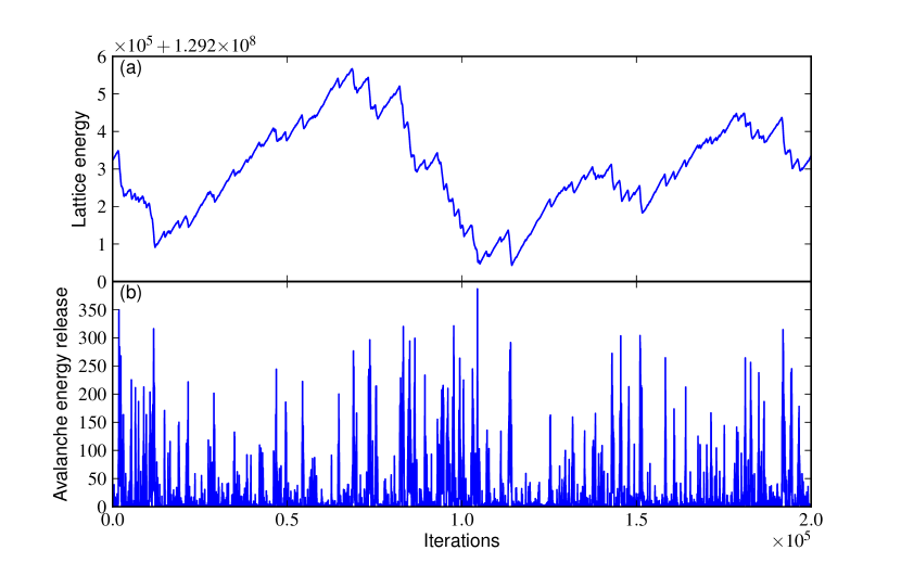
Figure 1.: Lattice energy (a) and avalanche energy release (b) time series for the LH model. Both energies are normalized to $e_{0}$.fig:lh_example

The total energy release (E), duration (T) and peak energy (P) of avalanches are distributed as a power-law over several decades (see the probability distribution functions – PDFs – in fig. fig:mod_properties). The D models have an anomalous non-power law component for very small avalanches, and model D3 also exhibit and small excess of large avalanches (for a complete discussion on these models, see Strugarek et al., 2014). In this work we assess the capability of avalanche models to predict large avalanche. Hence, the peculiar small avalanches population does not affect the results of this paper. The GV model possess a significantly different waiting time statistics (not shown here). Because of all these differences, we need to precisely define the time intervals and avalanches properties on which we characterize the predictive capabilities to ensure that some specificities of the models do not include some bias to our analysis. These definitions will naturally change from one model to the other (see section sec:predictive-abilities).

The five models are characterized by different power-law exponents, which are listed in table tab:props_mods. The power-law exponents characterizing the LH, GV and D3 models stand at the very low end of the observationally-inferred value for solar flares,  citep[e.g., $\alpha_{E}\in[1.39,1.78{]}$ in the hard X-rays data, see][]Aschwanden:2014wg, and fall significantly below this range for the D1 and D2 models. We will see that the predictive capabilities of the avalanches models are rather insensitive to these power-law exponents, but rather strongly depend on their embedded stochasticity Note that it is in principle possible to alter the components of the model to better reproduce the observationally-inferred power-law indices (see Charbonneau et al., 2001; Strugarek et al., 2014; Aschwanden et al., 2014).

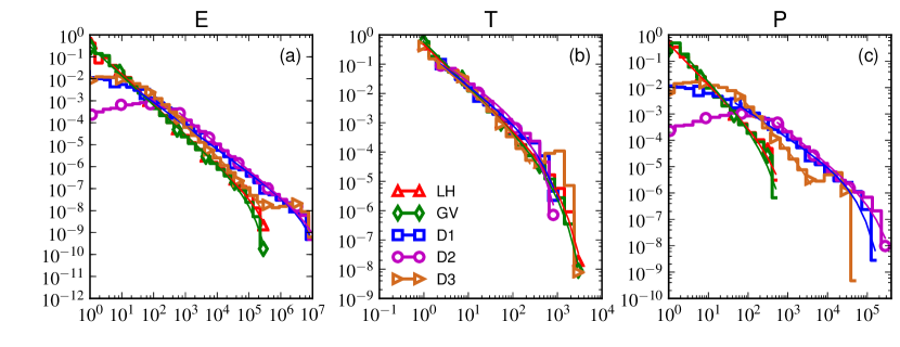
Figure 2.: Probability density functions of avalanches properties for the different models. The energy E (a), duration T (b) and peak energy P (c) of avalanches are shown. The power-law exponent for each quantity and each model are indicated in table tab:props_mods and the fits are plotted (solid lines).fig:mod_properties

	$E_{0}$	$\tau_{w}$	$\alpha_{E}$	$\alpha_{P}$	$\alpha_{T}$
LH	2 104	3.25 103	$1.37$	$1.53$	$1.45$
GV	2 104	1.5 103	$1.35$	$1.66$	$1.53$
D1	2 106	103	$1.07$	$1.00$	$1.21$
D2	2 106	1.5 103	$1.20$	$1.24$	$1.08$
D3	2 106	1.5 103	$1.39$	$1.63$	$1.28$

Table 1.: Statistical properties of the five models used for this study. The normalization energy and time windows are also indicated (see section sec:predictive-abilities). All models are defined on a 2D $48\times 48$ cartesian lattice with four-nearest-neighbour connectivity.tab:props_mods

4 Predictive Capabilities

sec:predictive-abilities

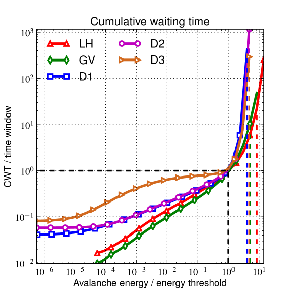
Figure 3.: Cumulative waiting time against avalanche energy (see text). Axis are normalized to the time window and energy threshold considered, which can vary from one model to one another.fig:time_properties

4.1 Prediction Time Windows

sec:pred-time-wind

Predicting the occurrence of an event requires the definition of the time window on which the prediction is given. The largest events – which we want to predict – are rare but obey specific statistical rules which depend on the avalanche model considered. We define a cumulative waiting time $\tau_{\rm CWT}(E)$ defined by the averaged waiting time between avalanches of energy higher than $E$. We display the cumulative waiting times as a function of the corresponding energy $E$ for the model we considered in fig. fig:time_properties. The D models have an almost-constant waiting-time distribution for the population of small avalanches (see Strugarek et al., 2014). Then, the models exhibit of a power-law part (except for model D3) followed by an exponential part for the highest energies. This change reflects the energy limit the avalanches can access due to the finite size of the lattices.

For each model, we identify the time window $\tau_{w}$ and its corresponding energy $E_{0}$ at which the slope of the cumulative waiting times changes (these quantities are model-dependent and are used to normalize the axes in figure fig:time_properties). We are interested in the capability of the models to predict the largest avalanches, hence we consider here avalanches of energy higher than $E_{0}$. We use in the following the time window $\tau_{w}$ to asses the predictive capabilities of the models. Because of the known statistical distribution of avalanches, most of the runs carried over $\tau_{w}$ will trigger at least an avalanche of energy $E_{0}$. In order to ensure that the predictive skills of the models are not the result of a simple statistical occurrence of an avalanche over $\tau_{w}$, we aim at determining the predictability of avalanches of energy $E_{p}$ (and higher) that statistically occur on time windows larger than $10\,\tau_{w}$. This will ensure that the observed avalanche results from a particular lattice state and/or a particular random number sequence (see section sec:mean-prediction-from), and is not the result of a climatological forecast based on the overall properties of the statistical SOC model (see also Barnes and Leka, 2008).

4.2 Predictions from Stochastic Models

sec:mean-prediction-from

Avalanche models always include a stochastic component, the realization of which varies from one run to one another. A prediction from a SOC-type model shall be composed of a sufficient number of runs varying the stochastic component of the model. Bearing in mind the analogy with solar flares prediction, we want to predict what will be the energy of the largest avalanche in the next $\tau_{w}$, and the time $\tau_{A}$ at which it will occur. For one fixed initial condition, we use $2000$ different random number sequences and store for each of them the starting time and release of energy of the largest avalanche over the time window. The resulting PDFs are shown in fig. fig:pred_example for the models LH, GV, D1 and D2 for a representative initial condition of each model (model D3 gives very similar results to D2).

The left panels display the PDF of the occurrence time of the largest avalanche in the time window, and the right panels the PDF of the largest avalanche energy. In all models, we notice that the energy is regularly distributed around a mean value. While the D models are well fitted by Gaussian (blue lines), the first two models have non-Gaussian tails. We chose to fit those resulting PDFs with a Weibull function which give satisfying fits (red lines). The best of the two fits is shown with a solid bulleted line and the other is shown in dashed thin line, for reference. The mean predicted value from the model is defined as the peak location of the best of the two fits. The fact that a mean can always be defined confirms the intuition that the stress pattern embedded in an instantaneous SOC state indeed determines the shape and size of upcoming avalanches, regardless of the stochastic component of the model. The departure of LH and GV models from a Gaussian behaviour nonetheless reveal an interesting property, which shall be confirmed in the following. We observe that the PDF is heavy tailed on the high energy side compared to a classical Gaussian distribution. On the one hand, the stochastic process tend to give the climatological prediction of the model ($E_{0}$, vertical solid grey line in fig. fig:pred_example). On the other hand, the initial stress pattern allows (or not) for very large avalanches to be triggered ($E_{\rm p}$, vertical dashed grey line). The heavy-tail part of the PDF directly derives from this latter property and is obtained only for a few favorable random number sequences, while the stochastic process is strong enough to severely alter the mean prediction towards the climatological forecast (vertical solid gray line). We clearly see that this property of the stochastic process is very strong in the LH and GV, and significantly weaker in models D. Hence, the Gaussian shape obtained in the D models simply indicative of marginal dependency upon the random number sequence: very large avalanche are triggered only when the adequate stress pattern exists in the lattice.

The left panels reveal another fundamental difference – in the context of predictability – between the models we considered. The LH and GV models show PDFs of $\tau_{A}$ spanning the whole time window, which means that the stochastic process determines when the largest avalanche will occur in the next time window. Hence, a mean $\tau_{A}$ is generally hard to define, although with some particular initial condition a slight peak value can be observed (not shown here). Conversely, the D models show PDFs peaked for a few values of $\tau_{A}$ which results in a very good confidence in the predicted time for the maximal avalanche. We note nonetheless that the multiplicity of peaks generally exhibited by the D1 model leads to a small but significant uncertainty on the occurrence time of the avalanche considered. Models D2 and D3 are the only models from which one can confidently predict an occurrence time.

The profound difference between the D models and the others is naturally explained by the deterministic character of their driving process. Being deterministic, the driver dictates unambiguously the next avalanching node which will be marginally affected by the choice of random number sequence (we recall here that in models D2 and D3, the stochastic process is only acting during avalanches and hence the driver completely determines the next avalanching node). If this node is likely to trigger a large avalanche, it will do so for most of the random number sequences. As a consequence, the PDF of $\tau_{A}$ for the D models will always be peaked. For small avalanches the stochastic elements embodied in the D models will significant impact the unfolding of a given avalanche, but for large avalanches, where many hundreds of nodes are involved – many avalanching repeatedly in the course of the same avalanche –, these stochastic fluctuations will tend to “even out” and have a limited impact on global avalanching characteristic, including the amount of released energy.

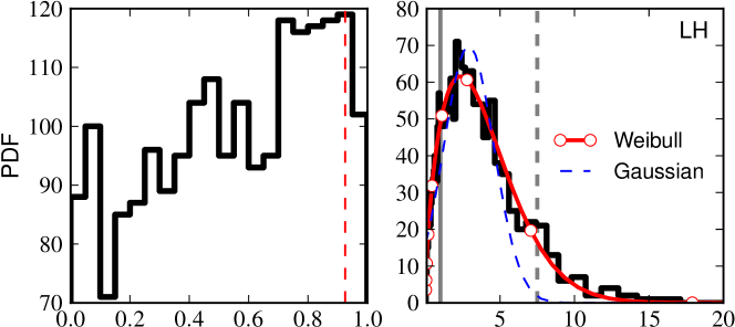
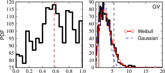
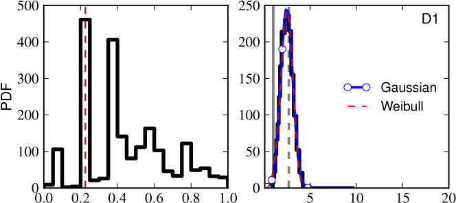
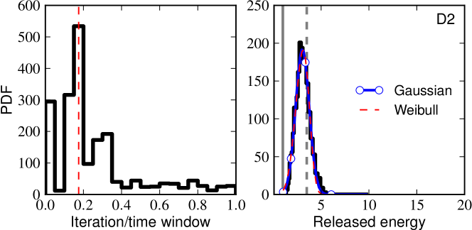
Figure 4.: Largest avalanche mean prediction from a set of $2000$ random number sequences using a common initial condition. Left panels display the PDFs of the predicted arrival time of the largest avalanche, and right panels the PDFs of the predicted energy. The peak $\tau_{a}$ is identified by a vertical red dashed line on left panels. The red and blue lines on the right panel label the Weibull and gaussian fits of the energy PDF. The solid and dashed vertical grey lines respectively label the normalization energy $E_{0}$ (the climatological forecast) and the target energy $E_{\rm p}$. Results from D3 (not shown here) closely resemble D2. fig:pred_example

4.3 Predictive Skills

sec:prediction-skills

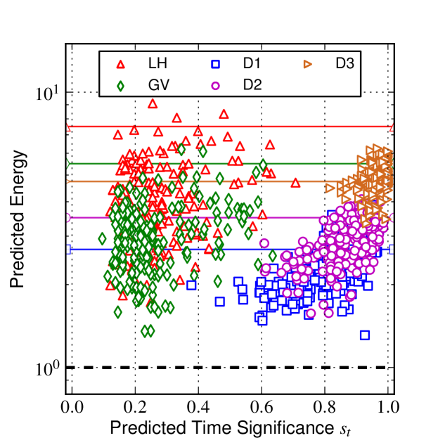
Figure 5.: Predictive capabilities of the models for $200$ independent events. The predicted energy (defined as the peak of the best fit of the PDF in the right panels of fig. fig:pred_example) is shown against the predicted time significance (see text). The closer the points are from unity, the higher the predictive capability. The dashed horizontal line corresponds to the climatological forecast of the model, the thin light lines correspond to the targeted energy $E_{p}$ for event prediction in each model.fig:combine_preds

We performed the statistical analysis described in section sec:mean-prediction-from for $200$ independent initial conditions – and associated large events – for each of the models. For each event, we define the predicted energy by the mean of the best fit to the PDF of the predicted avalanche energy. We also define the predicted time significance $s_{t}$ by estimating the significance of the largest peak in the $\tau_{A}$ distribution. A significance of $1$ corresponds to one and only one peak at one particular time, while a significance of $0$ corresponds to a purely flat PDF (see the top two left panels of fig. fig:pred_example). We display the results of the $200$ cases for the five models in fig. fig:combine_preds. The horizontal solid lines correspond to the values of $E_{\rm p}$, and the dashed line to the energy threshold. The intuition we got from fig. fig:pred_example is confirmed: the arrival time prediction is very good for D models ($s_{t}\gtrsim 0.5$), while LH and GV models rank poorly for almost all events ($s_{t}\lesssim 0.6$). The energy predicted by the LH and GV models lies in between the “climatological forecast” ($E_{0}$, dashed line) of the model and the target energy – which they almost never predict correctly. This implies that they are unable to predict reliably the very large avalanches. Conversely, large avalanches occurring in D models are generally recovered regardless the particular random sequence. Model D1 exhibits intermediate behavior with instances of both good and bad prediction, and model D3 performs extremely well, with $s_{t}>0.8$ for all the events considered here.

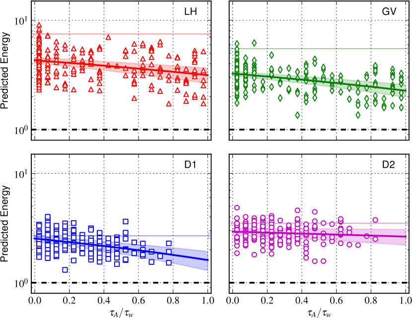
Figure 6.: The same data than in fig. fig:combine_preds is plotted against the occurrence time of the predicted avalanche, normalized to the prediction time window. The thick lines represent the best fit of the data (eqs. eq:fits_lin-eq:fits_lin_end), and the corresponding shaded areas the estimated error of the fit.fig:combine_preds2

Some events of the LH and GV models have good $s_{t}$ significance and the corresponding predicted energy is significantly larger than the other cases. They can be explained by taking a close look at fig. fig:combine_preds2 which displays the same results as on fig. fig:combine_preds but against the largest avalanche occurrence time (normalized to the time window) rather than $s_{t}$. The successfully predicted events of the LH and GV models correspond to runs where the large avalanches took place at the very beginning of the runs. Hence, they occurred in runs where almost no random numbers were involved, which is why they have very good predictive capability. We observe that the later the large avalanche occurs in the run, the lesser LH, GV and D1 models are able to predict an avalanche different from the climatological forecast (dashed line). The D2 model is, in contrast, predicting large avalanches fairly accurately regardless of the occurrence time in the prediction time window, again proving its high predictive capabilities. Finally, the D3 model (not shown here) exhibit almost no dependency of the event occurrence upon the time window. The dispersion of the predicted energies is nevertheless comparable in all the D models. To confirm this interpretation, we further fit a linear relation between $E/E_{0}$ and $\tau_{A}/\tau_{w}$ for each of the models (thick lines in Fig. fig:combine_preds2). We obtain, with energies normalized to $E_{0}$ for each model:

eq:fits_lin$$E_{\rm LH}/E_{0} = 4.30-1.16\,\frac{\tau_{A}}{\tau_{w}}\,,$$ (9)

$$E_{\rm GV}/E_{0} = 3.25-0.98\,\frac{\tau_{A}}{\tau_{w}}\,,$$ (10)

$$E_{\rm D1}/E_{0} = 2.54-0.92\,\frac{\tau_{A}}{\tau_{w}}\,,$$ (11)

$$E_{\rm D2}/E_{0} = 2.93-0.29\,\frac{\tau_{A}}{\tau_{w}}\,,$$ (12)

$$E_{\rm D3}/E_{0} = 4.8\,.$$ (13)

Again, only models D2 and D3 exhibit a small dependency of the predicted energy on the avalanche occurrence time $\tau_{A}$. The other models are clearly too sensitive to this parameter to be considered for reliable forecasts.

5 Conclusions

sec:conclusions

In this paper, we have assessed the predictive capabilities of a representative set of avalanches models for solar flares. Starting from the reference model of Lu & Hamilton, we modified the type of stochasticity embedded in the avalanche model and subsequently characterized their predictive capabilities. We focused our study on the prediction of large events, which are the rarest and presumably the hardest and most important to predict. We showed that only the purely deterministically driven model is able to predict a large event reliably, while the classical Lu & Hamilton model generally fails. We recall that the deterministically driven models show a deficit in term of small avalanches (Fig. fig:mod_properties) and hence depart from the classical SOC state. However, this property does not modify the predictive capabilities of the model, which were assessed for the larger, rarer avalanches, traditionally the hardest to predict.

Avalanche models always include the two conflicting aspects (in terms of predictive capabilities) of stochasticity and long-term correlations. By exploring the physical interpretation of avalanche models in the context of solar flares, we modified the stochastic process location in the model which lead to the development of a deterministically-driven model (Strugarek et al., 2014). We empirically demonstrated that this model possess the required properties to be used as a predictive tool: it is able to unambiguously predict the large avalanche occurrences over a given time window, well above the “climatological forecast”. We were able to demonstrate that the deterministically driven model has very little bias with the event occurrence time over a selected time-window. All the other models we considered are significantly affected by they stochastic component which makes them impossible to use for any practical prediction of large events. Computationally, avalanche models also have the significant advantage of being extremely inexpensive to run (this naturally results from their low dimensionality and their simplicity). Those unexpected properties promote a further investigation for the development of a near-real time prediction tool of large solar flares based on deterministically driven avalanche models. We envision this a a two-steps process.

First, as noted already the deterministically driven models considered here produce either power-law exponents (e.g., for the avalanche/flare energy distribution function) that are significantly lower than the real solar flare distribution exponents, or a small excess of large events. These different deterministically-driven models all possess good predictive capabilities for large events, which is probably one of their robust features. As a result, variations of the D model could be explored (e.g., in the spirit of Strugarek et al., 2014) to produce a model combining good predictive capabilities with statistical properties closer to the real solar flare data.

The second step consists in the coupling of data assimilation techniques (see, e.g. Bélanger, Vincent, and Charbonneau, 2007) to the chosen deterministically-driven model, and use observed times series (such as the Geostationary Operational Environmental Satellite – GOES X-ray time series) to assess quantitatively the predictive skills of the model (Barnes and Leka, 2008; Bloomfield et al., 2012). Our approach is complementary to the approach of Wheatland (2005) who also used the statistical properties of solar flare to predict the whole-Sun large events occurrence. In our case, the avalanche model can be viewed as a representation of one particular active region from which we will assimilate data. The use of selected data assimilation techniques will allow us to automatically adapt the driver and/or lattice state of the model, so that the output of the model matches the observed data. We show in figure fig:ex_DA an example of such data assimilation run using a simulated annealing method. The GOES flux (blue line in top panel) is transformed following to the method described in Aschwanden and Freeland (2012) into a distribution of delta-functions (black lines) filtered for flares of class C8 and above. We make the conversion of the GOES time sequence in terms of avalanche energy and model iterations using the typical waiting times of flares above C8 in model D3. In the bottom panel, we show three random realizations of model D3 (sets of light colored vertical lines) and one realization of model D3 using data assimilation (DA, red peaks) with the observed GOES time series (gray boxes). Here the assimilation technique succeeds in capturing the two clusters of flares exceeding C8 at $\simeq 25$ and $\simeq 60$  hr, without generating spurious ($\geq$ C8) flares before, after, or in between. The energy levels of the four reproduced flares also match very well with observations. The details of this assimilation technique will be described in details in Strugarek and Charbonneau (2014). These preliminary results suggest that the lattice configuration resulting from the data assimilation run combined with the predictive capabilities of the model we demonstrated in this work could be used to carry out quantitative predictions of solar flares through direct simulation. We believe that such a model could lead to significant improvements of the current predictions of large (typically X-class) solar flares.

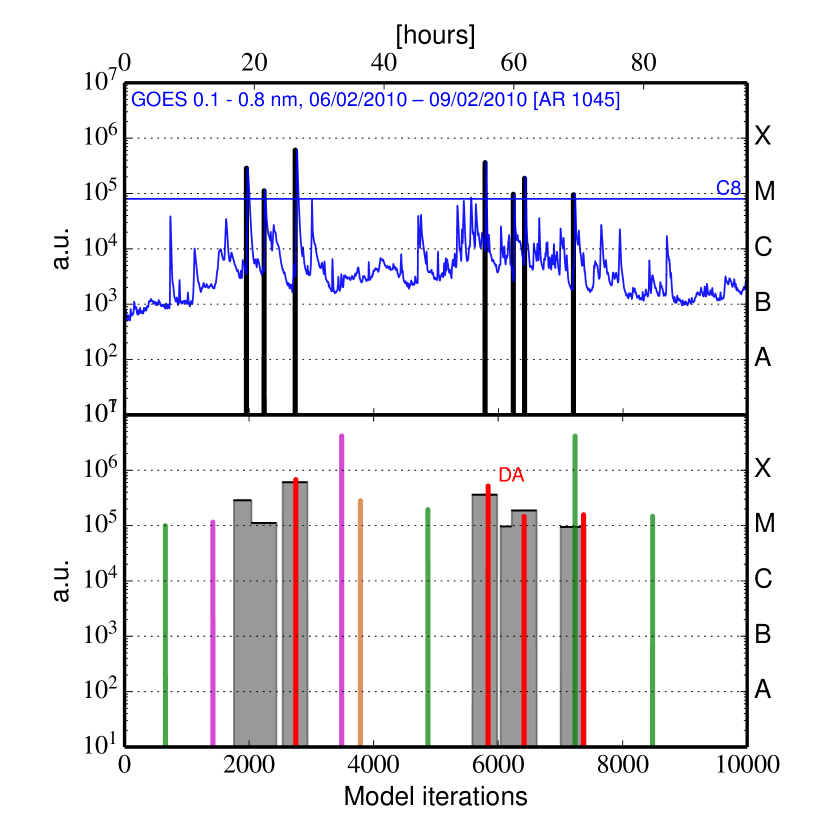
Figure 7.: Example of a run using data assimilation for the GOES flux in the $1$–$8$ $\dot{A}$ range during the flaring events of the active region 1045 between February 6 and February 9, 2010. The top panel show the GOES flux (blue) and the processed signal (see Aschwanden and Freeland, 2012) (black) for flares of class C8 and above. The bottom panel shows the GOES signal (grey boxes) used in the data assimilation run. The assimilated sequence (DA) is shown in red along with three random realizations of the model in orange, green and magenta.fig:ex_DA

Acknowledgements

The author thank the anonymous referee for valuable comments. The authors acknowledge stimulating discussions during the ISSI Workshops on Turbulence and Self-Organized Criticality (2012-2013) held in Bern (Switzerland); and during the “Festival de théorie” (2013) held in Aix-en-Provence (France). This research has made use of SunPy, an open-source and free community-developed solar data analysis package written in Python (Mumford et al., 2013). We also acknowledge support from the Natural Sciences and Engineering Research Council of Canada. AS acknowledges finanical support from CNES via SolarOrbiter grant.

References

- Aschwanden (2011) Aschwanden, M.J.: 2011, The State of Self-organized Criticality of the Sun During the Last Three Solar Cycles. I. Observations. Sol. Phys. 274(1), 99. DOI. ADS.
- Aschwanden and Charbonneau (2002) Aschwanden, M.J., Charbonneau, P.: 2002, Effects of Temperature Bias on Nanoflare Statistics. ApJ 566(1), L59. DOI. ADS.
- Aschwanden and Freeland (2012) Aschwanden, M.J., Freeland, S.L.: 2012, Automated Solar Flare Statistics in Soft X-Rays over 37 Years of GOES Observations: The Invariance of Self-organized Criticality during Three Solar Cycles. ApJ 754(2), 112. DOI. ADS.
- Aschwanden and McTiernan (2010) Aschwanden, M.J., McTiernan, J.M.: 2010, Reconciliation of Waiting Time Statistics of Solar Flares Observed in Hard X-rays. ApJ 717(2), 683. DOI. ADS.
- Aschwanden and Parnell (2002) Aschwanden, M.J., Parnell, C.E.: 2002, Nanoflare Statistics from First Principles: Fractal Geometry and Temperature Synthesis. ApJ 572(2), 1048. DOI. ADS.
- Aschwanden et al. (2014) Aschwanden, M.J., Crosby, N., Dimitropoulou, M., Georgoulis, M.K., Hergarten, S., McAteer, R.T.J., Milovanov, A., Mineshige, S., Morales, L., Pruessner, G., Sanchez, R., Strugarek, A., Uritsky, V.: 2014, 25 Years of Self-Organized Criticality: Solar and Astrophysics. Space Science Reviews, in press.
- Bak, Tang, and Wiesenfeld (1987) Bak, P., Tang, C., Wiesenfeld, K.: 1987, Self-organized criticality - An explanation of 1/f noise. Phys. Rev. Lett. 59, 381. DOI. ADS.
- Barnes and Leka (2008) Barnes, G., Leka, K.D.: 2008, Evaluating the Performance of Solar Flare Forecasting Methods. ApJ 688(2), L107. DOI. ADS.
- Bélanger, Vincent, and Charbonneau (2007) Bélanger, E., Vincent, A., Charbonneau, P.: 2007, Predicting Solar Flares by Data Assimilation in Avalanche Models. I. Model Design and Validation. Sol. Phys. 245(1), 141. DOI. ADS.
- Bloomfield et al. (2012) Bloomfield, D.S., Higgins, P.A., McAteer, R.T.J., Gallagher, P.T.: 2012, Toward Reliable Benchmarking of Solar Flare Forecasting Methods. ApJ 747(2), L41. DOI. ADS.
- Charbonneau (2013) Charbonneau, P.: 2013, SOC and Solar Flares. In: Self-Organized Criticality Systems, Open Academic Press, 404. ADS.
- Charbonneau et al. (2001) Charbonneau, P., McIntosh, S.W., Liu, H.-L., Bogdan, T.J.: 2001, Avalanche models for solar flares (Invited Review). Sol. Phys. 203(2), 321. DOI. ADS.
- Chen (2011) Chen, P.F.: 2011, Coronal Mass Ejections: Models and Their Observational Basis. Living Rev. Solar Phys. 8, 1. DOI. ADS.
- Georgoulis (2012) Georgoulis, M.K.: 2012, On Our Ability to Predict Major Solar Flares. The Sun: New Challenges 3, 93. DOI. ADS.