The multivariate Dirichlet-multinomial distribution
and its application in forensic genetics to adjust for sub-population effects using the $\theta$-correction

Abstract

In this paper, we discuss the construction of a multivariate generalisation of the Dirichlet-multinomial distribution. An example from forensic genetics in the statistical analysis of DNA mixtures motivates the study of this multivariate extension.

In forensic genetics, adjustment of the match probabilities due to remote ancestry in the population is often done using the so-called $\theta$-correction. This correction increases the probability of observing multiple copies of rare alleles and thereby reduces the weight of the evidence for rare genotypes.

By numerical examples, we show how the $\theta$-correction incorporated by the use of the multivariate Dirichlet-multinomial distribution affects the weight of evidence. Furthermore, we demonstrate how the $\theta$-correction can be incorporated in a Markov structure needed to make efficient computations in a Bayesian network. Keywords: Multivariate Dirichlet-multinomial distribution; STR DNA mixture; Forensic genetics; $\theta$-correction

1 Introduction

When biological material is obtained from a scene of crime, it is often possible to produce a DNA profile from even minute amounts of DNA. In cases where DNA from more than one individual is present in the resulting DNA profile, the DNA profile is called a DNA mixture. DNA mixtures are harder to interpret and analyse than single contributor stains as there are many sources of uncertainty, e.g. the number of contributors, the relative amounts of contributed DNA and the individual DNA profiles of the contributors. For more than twenty years (Evett et al., 1991), statistical modelling of DNA mixtures has attracted much attention. The statistical models have been extended to cope with more of the uncertainties and artifacts observed in the detected mixed DNA profile. Modelling these components is important in order to assess the probability of the evidence, since it is the task of the forensic geneticists to assign an evidential weight by computing the likelihoods of the evidence under competing hypotheses.

Recently, Cowell et al. (2015) published a statistical model for DNA mixtures, which in a coherent framework enabled the modelling of common phenomena as stutters (artefacts of the polymerase chain reaction, PCR), allelic drop-out (undetected alleles of the true contributors) and silent alleles (unobservable alleles, e.g. due to mutations in primer binding regions). In order to estimate the model parameters, the authors maximised the likelihood under each hypothesis. Due to the vast number of possible combinations of DNA profiles, this is computationally demanding and challenging. However, the methodology of Cowell et al. (2015) and its implementation (R-package DNAmixtures, Graversen, 2014) solved this by utilising Bayesian networks and the implementation of these in the Hugin Software (http://www.hugin.com).

As future work, Cowell et al. (2015, Section 5.3.2) suggested to implement a correction for subpopulation effects on the allele probabilities. In order to correct for these subpopulation structures, Nichols and Balding (1991) suggested the “$\theta$-correction” to be used when inferring the weight of evidence in forensic genetics. The Markov structure for representing the individual genotypes in Cowell et al. (2015) imposed to conform with the Bayesian network paradigm did not allow for incorporating correlation between the individual DNA profiles (see Fig. 1 below and also Fig. 4 of Cowell et al., 2015).

Here, we show how this Markov structure can be modified in order to incorporate positive correlations between alleles within and among the genotypes involved. A consequence of positive correlation is an increased probability of homozygosity, which may be induced by subpopulation structures in the population.

The resulting distribution when incorporating the $\theta$-correction for multiple contributors in a Bayesian network framework is a multivariate generalisation of the Dirichlet-multinomial distribution. The Dirichlet-multinomial distribution was first derived by Mosimann (1962), who derived it as a compound distribution in which the probability vector of a multinomial distribution is assumed to follow a Dirichlet distribution (Mosimann, 1962). After marginalisation over this distribution, the cell counts follow a Dirichlet-multinomial distribution (Mosimann, 1962; Johnson et al., 1997).

The present paper is structured as follows: In Section 2, we discuss how the $\theta$-correction is implemented for a single DNA profile. In Section 3, this is generalised for more contributors. This multiple contributor extension of the genotype model leads to the introduction of the multivariate Dirichlet-multinomial distribution. In Section 4, we derive the structures of the marginal and conditional distributions of the multivariate Dirichlet-multinomial distribution. Furthermore, the expression of the generalised factorial moments is derived, which is used to obtain the mean and covariance matrix of the distribution. In Section 5, we show by numerical examples how the $\theta$-correction affects the weight of the evidence.

2 Dirichlet-multinomial distribution

In order to adjust for genetic subpopulation structures when computing the weight of evidence in forensic genetics, it is common to use the $\theta$-correction (Balding and Nichols, 1994). Several authors have discussed the interpretation of $\theta$; Curran et al. (1999, 2002) derived likelihood ratio expressions with $\theta$ being the probability that a pair of alleles is identical-by-descent (IBD). Tvedebrink (2010) defined $\theta$ as an overdispersion parameter in a multinomial sampling scheme, and Green and Mortera (2009) discussed $\theta$ in relation to assumptions made about founding genes in populations.

In forensic genetics, the prevailing genotyping technology is based on short tandem repeat (STR) loci. The genotype at a given STR locus is represented by a pair of alleles, each of which is inherited from the individual’s parents. Let $A$ denote the possible number of alleles, typically in the range of five to 20, at a given STR locus. The genotype of individual $i$ can be represented as a vector of allele counts, $\bm{n}_{i}$, where $n_{ia}$ is the number of $a$ alleles of the genotype. By forming a cumulative sum, $S_{ia}=\sum_{b=1}^{a}n_{ia}$, of allele counts, $n_{ia}$, for alleles $a\in\{1,\dots,A\}$, Graversen and Lauritzen (2014) showed that the multinomial distribution over allele counts for unknown contributors may be evaluated by the product of a sequence of binomial distributions (see Fig. 1) such that $n_{ia}\mid S_{i,a-1}\sim\text{bin}(2-S_{i,a-1},Q_{a})$, where $Q_{a}=q_{a}/\sum_{b=a}^{A}q_{b}$.

Fig. 1: Markov structure of allele counts of contributor $i$ for a marker with six possible alleles.

If the distribution of allele probabilities is assumed to follow a Dirichlet distribution, then the marginal distribution of allele counts under a multinomial sampling scheme follows a Dirichlet-multinomial distribution (Tvedebrink, 2010). Using similar derivations as in Graversen and Lauritzen (2014), we show that the $\theta$-correction can be incorporated by evaluating the Dirichlet-multinomial distribution by a sequence of beta-binomial distributions.

Let $n=\sum_{b=1}^{A}n_{b}$ and suppress the subscript $i$, then the Dirichlet-multinomial distribution can be specified by

$$P(n_{1},\dots,n_{A})=\frac{n!\Gamma(\alpha_{\bullet})}{\Gamma(n+\alpha_{\bullet})}\prod_{b=1}^{A}\left\{\frac{\Gamma(n_{b}+\alpha_{b})}{n_{b}!\Gamma(\alpha_{b})}\right\},$$

where $\alpha_{\bullet}=\sum_{b=1}^{A}\alpha_{b}$ and $\bm{\alpha}=(\alpha_{1},\dots,\alpha_{A})$ being positive real valued parameters (Johnson et al., 1997). The joint distribution over sums of disjoint subsets of cell counts is also Dirichlet-multinomial (Johnson et al., 1997, pp. 81). In particular, when collapsing the last $A-a$ cells into one cell it will yield a parameter-vector of $(\alpha_{1},\dots,\alpha_{a},\alpha_{\bullet{a{+}1}})$ with $\alpha_{\bullet{a{+}1}}=\sum_{b=a{+}1}^{A}\alpha_{b}$. In the case where $\bm{n}$ denotes the allele counts, $n=2$ and the distribution of allele counts $(n_{1},\dots,n_{a})$, $a\in\{1,\dots,A{-}1\}$ is given by:

$$P(n_{1},\dots,n_{a})=\frac{2!\Gamma(\alpha_{\bullet})}{\Gamma(2{+}\alpha_{\bullet})}\frac{\Gamma(2{-}S_{a}{+}\alpha_{\bullet{a{+}1}})}{(2{-}S_{a})!\Gamma(\alpha_{\bullet{a{+}1}})}\prod_{b=1}^{a}\left\{\frac{\Gamma(n_{b}{+}\alpha_{b})}{n_{b}!\Gamma(\alpha_{b})}\right\}.$$

Using this result, we obtain the conditional distribution of $n_{a}$ given $n_{1},\dots,n_{a-1}$ as

$$P(n_{a}\,|\,n_{a{-}1}\dots,n_{1}) =\frac{P(n_{a},n_{a{-}1}\dots,n_{1})}{P(n_{a{-}1}\dots,n_{1})}$$

$$=\dfrac{\dfrac{2!\Gamma(\alpha_{\bullet})}{\Gamma(2+\alpha_{\bullet})}\dfrac{\Gamma(2-S_{a}+\alpha_{\bullet{a{+}1}})}{(2-S_{a})!\Gamma(\alpha_{\bullet{a{+}1}})}\prod\limits_{b=1}^{a}\left\{\dfrac{\Gamma(n_{b}+\alpha_{b})}{n_{b}!\Gamma(\alpha_{b})}\right\}}{\dfrac{2!\Gamma(\alpha_{\bullet})}{\Gamma(2+\alpha_{\bullet})}\dfrac{\Gamma(2-S_{a{-}1}+\alpha_{\bullet{a}})}{(2-S_{a{-}1})!\Gamma(\alpha_{\bullet{a}})}\prod\limits_{b=1}^{a-1}\left\{\dfrac{\Gamma(n_{b}+\alpha_{b})}{n_{b}!\Gamma(\alpha_{b})}\right\}}$$

$$={2{-}S_{a{-}1}\choose n_{a}}\frac{\Gamma(\alpha_{\bullet{a{+}1}}+\alpha_{a})}{\Gamma(\alpha_{a})\Gamma(\alpha_{\bullet{a{+}1}})}\frac{\Gamma(n_{a}{+}\alpha_{a})\Gamma(2{-}S_{a{-}1}{-}n_{a}+\alpha_{\bullet{a{+}1}})}{\Gamma(2{-}S_{a{-}1}+\alpha_{\bullet{a{+}1}}+\alpha_{a})},$$

where from the second to the third line, we used that $S_{a}=S_{a{-}1}+n_{a}$ and $\alpha_{\bullet{a{+}1}}=\alpha_{\bullet{a}}-\alpha_{a}$. This is a beta-binomial distribution (Johnson et al., 1997, pp. 81) with parameters $(2-S_{a-1},\alpha_{a},\alpha_{\bullet{a{+}1}})$ that are similar to those of the binomial distribution $(2-S_{a-1},Q_{a})$. Similarly to Graversen and Lauritzen (2014), we observe directly from the expression that $n_{a}\perp\!\!\!\perp(n_{1},\dots,n_{a-1},S_{1},\dots,S_{a-2})\mid S_{a-1}$. Finally, we note that the allele probabilities $\bm{q}=(q_{1},\dots,q_{A})$ and $\theta$ are related to $\bm{\alpha}$ through $q_{a}=\alpha_{a}/\alpha_{\bullet}$ and $\theta=(1+\alpha_{\bullet})^{-1}$ (Tvedebrink, 2010).

3 Multivariate Dirichlet-multinomial distribution

When incorporating the $\theta$-correction for more contributors, it is necessary to modify the Markov structure in Fig. 1 as we need to model the joint distribution of $n_{ia}$ and $n_{ja}$ in order to incorporate the positive correlation from remote ancestry. Thus, the Markov structure depicted in Cowell et al. (2015, Fig. 4) should be replaced by the Markov structure in Fig. 2.

Fig. 2: Extended Markov structure for incorporating $\theta$-correction for two contributors. As in Fig. 1, there are six possible alleles, where $Q_{a}$ denotes the scaled allele probabilities. For profile $i$, the allele counts and cumulative sums are given by $(n_{ia},S_{ia})$, and similarly $(n_{ja},S_{ja})$ for profile $j$. The $O_{a}$ nodes have the same meaning as in Cowell et al. (2015). The dashed box represents the clique necessary to propagate in the Bayesian network.

In Fig. 2, the distribution of the allele probabilities, $q_{a}$, was modelled by a Dirichlet distribution. This distribution can be specified sequentially by the following relation: $Q_{a}\sim\text{beta}(\alpha_{a},\alpha_{\bullet{a{+}1}})$, where $Q_{a}=q_{a}/\sum_{b=a}^{A}$ for $a=1,\dots,A{-}1$. Furthermore, these beta-distributions are mutually independent (Johnson et al., 1997), which implies that the Dirichlet distribution can be formulated as a product of beta distributions.

First, we observe that, conditioned on $Q_{a}$ and cumulative sums, the allele counts from the two individuals are mutually independent:

$$P(n_{ia},n_{ja}\mid S_{i,a{-}1},S_{j,a{-}1},Q_{a}) =P(n_{ia}\mid S_{i,a{-}1},Q_{a})P(n_{ja}\mid S_{j,a{-}1},Q_{a})$$

$$={2{-}S_{i,a{-}1}\choose n_{ia}}{2{-}S_{j,a{-}1}\choose n_{ja}}Q_{a}^{n_{\bullet a}}(1-Q_{a})^{4-S_{\bullet a{-}1}-n_{\bullet a}},$$

where $n_{\bullet a}=n_{ia}+n_{ja}$ and $S_{\bullet a{-}1}=S_{i,a{-}1}+S_{j,a{-}1}$. Secondly, we marginalise over $Q_{a}$, which is beta distributed with parameters $(\alpha_{a},\alpha_{\bullet{a{+}1}})$:

$$\int_{0}^{1}P(n_{ia}\mid S_{i,a{-}1},Q_{a})P(n_{ja}\mid S_{j,a{-}1},Q_{a})f(Q_{a})\,\text{d}Q_{a}\\ ={2{-}S_{i,a{-}1}\choose n_{ia}}{2{-}S_{j,a{-}1}\choose n_{ja}}\frac{\Gamma({\alpha_{\bullet}}_{a})}{\Gamma(\alpha_{a})\Gamma(\alpha_{\bullet{a{+}1}})}\int_{0}^{1}Q_{a}^{n_{\bullet a}+\alpha_{a}-1}(1-Q_{a})^{4-S_{\bullet a{-}1}-n_{\bullet a}+\alpha_{\bullet{a{+}1}}-1}\,\text{d}Q_{a},$$

which is the integral of a non-normalised beta-distribution. By letting $S_{i0}=S_{j0}=0$, we have for $1\leq a<A$ that $P(n_{ia},n_{ja}\mid S_{i,a{-}1},S_{j,a{-}1})$ is given by:

$${2{-}S_{i,a{-}1}\choose n_{ia}}{2{-}S_{j,a{-}1}\choose n_{ja}}\frac{\Gamma({\alpha_{\bullet}}_{a})}{\Gamma(\alpha_{a})\Gamma(\alpha_{\bullet{a{+}1}})}\frac{\Gamma(n_{\bullet a}+\alpha_{a})\Gamma(4-S_{\bullet a{-}1}-n_{\bullet a}+\alpha_{\bullet{a{+}1}})}{\Gamma(4-S_{\bullet a{-}1}+{\alpha_{\bullet}}_{a})}.$$ (1)

A consequence of marginalising over $Q_{a}$ is that the clique size in the network decreases. For the two profiles in Fig. 2, this marginalisation implies that the relevant clique size decreases from eight to six nodes as $Q_{a{-}1}$ and $Q_{a}$ are removed, while the imposed correlation connects the nodes $n_{ia}$ and $n_{ja}$ (graph not shown).

In the general setting, where we consider a DNA mixture of $I$ contributors, we denote $\bm{n}=(\bm{n}_{1},\dots,\bm{n}_{I})$, where each $\bm{n}_{i}=(n_{i1},\dots,n_{iA})$ denotes the allele counts for profile $i$ and, similarly, for the cumulative sums, $S_{ia}=\sum_{b=1}^{a}n_{ib}$. Hence, $P(n_{1a},\dots,n_{Ia}\mid S_{1,a{-}1},\dots,S_{I,a{-}1})$ is given by

$$\left\{\prod_{i=1}^{I}{2{-}S_{i,a{-}1}\choose n_{ia}}\right\}\frac{\Gamma({\alpha_{\bullet}}_{a})}{\Gamma(\alpha_{a})\Gamma(\alpha_{\bullet{a{+}1}})}\frac{\Gamma(n_{\bullet a}+\alpha_{a})\Gamma(2I-S_{\bullet a{-}1}-n_{\bullet a}+\alpha_{\bullet{a{+}1}})}{\Gamma(2I-S_{\bullet a{-}1}+{\alpha_{\bullet}}_{a})},$$

where $n_{\bullet a}=\sum_{i=1}^{I}n_{ia}$ and $S_{\bullet a{-}1}=\sum_{i=1}^{I}S_{i,a{-}1}$.

In full generality, consider a set of vectors $\bm{n}=(\bm{n}_{1},\dots,\bm{n}_{I})$, where $\bm{n}_{i}=(n_{i1},\dots,n_{iA})$ and $n_{i\bullet}=\sum_{a=1}^{A}n_{ia}$ for $n_{i\bullet}\in\mathbb{Z}_{0}$. Then the probability mass function for $\bm{n}$ is given by

$$P(\bm{n})=\left\{\prod_{i=1}^{I}{n_{i\bullet}\choose\bm{n}_{i}}\right\}\frac{\Gamma(\alpha_{\bullet})}{\Gamma(n_{\bullet\bullet}+\alpha_{\bullet})}\prod_{a=1}^{A}\frac{\Gamma(n_{\bullet a}+\alpha_{a})}{\Gamma(\alpha_{a})},$$ (2)

where $n_{\bullet\bullet}=\sum_{a=1}^{A}n_{\bullet a}=\sum_{a=1}^{A}\sum_{i=1}^{I}n_{ia}$. For a single contributor, i.e. $I=1$ and $\bm{n}=(n_{1},\dots,n_{A})$, this distribution simplifies to the Dirichlet-multinomial distribution. Hence, we may call this distribution the multivariate Dirichlet-multinomial (MDM) distribution, which we denote $\text{\sl MDM}(\bm{n}_{*\bullet},\bm{\alpha})$, where $\bm{n}_{*\bullet}=(n_{1\bullet},\dots,n_{i\bullet},\dots,n_{I\bullet})$ is the vector of trails per experiment (row sums in Table 1) or e.g. the number of alleles per DNA profile. Furthermore, we observe from (2) that inference about the model parameters, $\bm{\alpha}$, only depends on $\bm{n}_{\bullet*}=(n_{\bullet 1},\dots,n_{\bullet a},\dots,n_{\bullet A})$, i.e. the column sums shown in Table 1.

Table 1: Sufficient statistics of a table when modelled using the multivariate Dirichlet-multinomial (MDM) distribution. By construction of the MDM distribution, the row sums, $n_{i\bullet}$, and the total sum, $n_{\bullet\bullet}$, are known and fixed.

	$1$	$\dots$	$a$	$\dots$	$A$
$1$	$n_{11}$	$\dots$	$n_{1a}$	$\dots$	$n_{1A}$	$n_{1\bullet}$
$\vdots$	$\vdots$	$\ddots$	$\vdots$	$\ddots$	$\vdots$	$\vdots$
$i$	$n_{i1}$	$\dots$	$n_{ia}$	$\dots$	$n_{iA}$	$n_{i\bullet}$
$\vdots$	$\vdots$	$\ddots$	$\vdots$	$\ddots$	$\vdots$	$\vdots$
$I$	$n_{I1}$	$\dots$	$n_{Ia}$	$\dots$	$n_{IA}$	$n_{I\bullet}$
	$n_{\bullet 1}$	$\dots$	$n_{\bullet a}$	$\dots$	$n_{\bullet A}$	$n_{\bullet\bullet}$

To emphasise the difference between row and column marginals, we let $\bm{n}_{\bullet*}=(n_{\bullet 1},\dots,n_{\bullet a},\dots,n_{\bullet A})$ denote the column sums, which we shall use in the next section when discussing conditional and marginal distributions.

Furthermore, let $B\subset\{1,\dots,A\}$ be a subset of the cells, e.g. a subset of the alleles in a genetics context, and let $C$ denote the complement of $B$. The counts associated with $B$, $C$ and the row sums over $C$ are defined by

$$\bm{n}_{*B}=\{n_{ia}\}_{a\in B},~{}~{}\bm{n}_{*C}=\{n_{ia}\}_{a\in C}~{}~{}\text{and}~{}~{}\bm{n}_{*\bullet}^{(C)}=\left\{\sum\nolimits_{a\in C}n_{ia}\right\}~{}~{}\text{for}~{}~{}i=1,\dots,I,\text{~{}respectively.}$$

Similarly, we may consider subsetting over index $i$ such that $J$ and $K$ specify two disjoint and exhaustive partitions of $\{1,\dots,i,\dots,I\}$, where $\bm{n}_{J*}$ and $\bm{n}_{K*}$ denote the counts, respectively. In the DNA mixture context, this corresponds to partition of the set of $I$ contributors into two disjoint groups.

4 Properties of multivariate Dirichlet-multinomial distribution

4.1 Conditional and marginal distributions

The construction of the MDM distribution implies that it carries many similarities to the Dirichlet-multinomial distribution. For the MDM distribution, one may consider marginalisation and conditioning over both $i$ and $a$ in the $n_{ia}$ notation. Furthermore, we may also condition on $\bm{n}_{\bullet*}$ and $\bm{n}_{*\bullet}$ to obtain a generalisation of the hypergeometric distribution.

First, we consider the marginal and conditional distribution over index $a$: The marginal distribution of $\bm{n}_{*B}$ can be thought of as the distribution when collapsing all elements of $C$ into one hyper-class (or allele). By using similar arguments as Johnson et al. (1997, pp. 81), this gives the results that the marginal and conditional distributions are MDM with parameters given by

$$\bm{n}_{*B}\sim\text{\sl MDM}(\bm{n}_{*\bullet},\{\bm{\alpha}_{B},\alpha_{C}\})\quad\text{and}\quad\bm{n}_{*B}\mid\bm{n}_{*C}\sim\text{\sl MDM}(\bm{n}_{*\bullet}-\bm{n}_{*\bullet}^{(C)},\bm{\alpha}_{B}),$$

where $\bm{\alpha}_{B}=\{\alpha_{a}\}_{a\in B}$ and $\alpha_{C}=\sum_{a\in C}\alpha_{a}$.

Secondly, we handle the case of marginalising and conditioning over index $i$. It follows directly from (2) that the distribution of $\bm{n}_{J*}$ is MDM with parameters $\bm{n}_{J\bullet}$ and $\bm{\alpha}$, where $\bm{n}_{J\bullet}=\{n_{i\bullet}\}_{i\in J}$. The conditional distribution of $\bm{n}_{J*}$ given $\bm{n}_{K*}$ can be considered as a posterior distribution as we have already observed counts $\bm{n}_{K*}$, which are then factorised into the parameters. Thus, we have

$$\bm{n}_{J*}\sim\text{\sl MDM}(\bm{n}_{J\bullet},\bm{\alpha})\quad\text{and}\quad\bm{n}_{J*}\mid\bm{n}_{K*}\sim\text{\sl MDM}(\bm{n}_{J\bullet},\bm{\alpha}+\bm{n}_{\bullet*}^{(K)}),$$

where $\bm{n}_{\bullet*}^{(K)}=\{\sum_{i\in K}n_{ia}\}$ for $a=1,\dots,A$, i.e. the number of $a$ alleles observed for the profiles in $K$.

Finally, when conditioning on the sufficient statistic, $\bm{n}_{\bullet*}$, and the number trails, $\bm{n}_{*\bullet}$, we recover the results for contingency tables that $n_{**}\mid(\bm{n}_{\bullet*},\bm{n}_{*\bullet})$ follow a generalisation of the multivariate-hypergeometric distribution (Johnson et al., 1997) with parameters $\bm{n}_{\bullet*}$ and $\bm{n}_{*\bullet}$:

$$P(\bm{n};\bm{n}_{\bullet*},\bm{n}_{*\bullet})=\dfrac{\prod_{i=1}^{I}{n_{i\bullet}\choose\bm{n}_{i}}}{{n_{\bullet\bullet}\choose\bm{n}_{\bullet*}}}=\dfrac{\prod_{i=1}^{I}n_{i\bullet}!\prod_{a=1}^{A}n_{\bullet a}!}{n_{\bullet\bullet}!\prod_{i=1}^{I}\prod_{a=1}^{A}n_{ia}!},$$

which is identical to Halton’s “exact contingency formula” (Halton, 1969) and utilised in Patefield’s algorithm (Patefield, 1981) to generate $R\times C$ contingency tables.

4.2 Moments

In Appendix A, we show that the moments of MDM can be computed using the generalised factorial moments which are given by:

$$\mathbb{E}\left(\bm{n}^{(\bm{r})}\right)=\mathbb{E}\left\{\prod_{i=1}^{I}\prod_{a=1}^{A}n_{ia}^{(r_{ia})}\right\}=\left\{\prod\limits_{i=1}^{I}\frac{n_{i\bullet}!}{(n_{i\bullet}{-}r_{i\bullet})!}\right\}\dfrac{\prod\limits_{a=1}^{A}\prod\limits_{k=0}^{r_{\bullet a}{{-}}1}(\alpha_{a}{+}k)}{\prod\limits_{k=0}^{r_{\bullet\bullet}{{-}}1}(\alpha_{\bullet}{+}k)},$$ (3)

where $a^{(b)}=a(a-1)\cdots(a-b+1)=a!/(a-b)!$ is a rising factorial. Hence, in order to compute the mean of $n_{ia}$, we set $r_{ia}=1$ and $r_{\bullet\bullet}=1$ (implying that $r_{i\bullet}=1$ and $r_{\bullet a}=1$). Plugging this into (3), we obtain $\mathbb{E}(n_{ia})=n_{i\bullet}\alpha_{a}/\alpha_{\bullet}=n_{i\bullet}q_{a}$, as expected. Furthermore, the covariance matrix can be computed for the different levels of correlations (left: within individual $i$, and right: between individuals $i$ and $i^{\prime}$):

$$\mathbb{C}ov(n_{ia},n_{ia}) =n_{i\bullet}q_{a}(1{-}q_{a})[1+(n_{i\bullet}{-}1)\theta] \mathbb{C}ov(n_{ia},n_{i^{\prime}a}) =n_{i\bullet}n_{i^{\prime}\bullet}q_{a}(1{-}q_{a})\theta$$

$$\mathbb{C}ov(n_{ia},n_{ia^{\prime}}) =-n_{i\bullet}q_{a}q_{a^{\prime}}[1+(n_{i\bullet}{-}1)\theta] \mathbb{C}ov(n_{ia},n_{i^{\prime}a^{\prime}}) =-n_{i\bullet}n_{i^{\prime}\bullet}q_{a}q_{a^{\prime}}\theta,$$

where $\mathbb{C}ov(n_{ia},n_{ia})=\mathbb{V}ar(n_{ia})$. In the case where $\bm{n}_{i}$ represents a DNA profile, we have for all $i$ that $n_{i\bullet}=2$. Thus, in this particular case we obtain:

$$\mathbb{C}ov(n_{ia},n_{ia}) =2q_{a}(1{-}q_{a})[1+\theta] \mathbb{C}ov(n_{ia},n_{i^{\prime}a}) =4q_{a}(1{-}q_{a})\theta$$

$$\mathbb{C}ov(n_{ia},n_{ia^{\prime}}) =-2q_{a}q_{a^{\prime}}[1+\theta] \mathbb{C}ov(n_{ia},n_{i^{\prime}a^{\prime}}) =-4q_{a}q_{a^{\prime}}\theta,$$

which implies positive correlation between counts of identical alleles within and between individuals. Consequently, for different alleles the correlation is negative.

5 Numerical results

In order to demonstrate how the $\theta$-correction affects $P(\bm{n}|\mathcal{H})$ in the evaluation of the $L(\mathcal{H})$ expression of Equation 8 in Cowell et al. (2015), we evaluate

$$\text{\sl WoE}(n_{\bullet a},S_{\bullet a{-}1};Q_{a},\theta) =\frac{P(n_{ia}\mid S_{i,a{-}1};Q_{a})P(n_{ja}\mid S_{j,a{-}1};Q_{a})}{P(n_{ia},n_{ja}\mid S_{i,a{-}1},S_{j,a{-}1};Q_{a},\theta)}$$

$$=\frac{Q_{a}^{n_{\bullet a}}(1{-}Q_{a})^{4{-}S_{\bullet a{-}1}{-}n_{\bullet a}}}{\dfrac{\Gamma({\alpha_{\bullet}}_{a})}{\Gamma(\alpha_{a})\Gamma(\alpha_{\bullet{a{+}1}})}\dfrac{\Gamma(n_{\bullet a}{+}\alpha_{a})\Gamma(4{-}S_{\bullet a{-}1}{-}n_{\bullet a}{+}\alpha_{\bullet{a{+}1}})}{\Gamma(4{-}S_{\bullet a{-}1}{+}{\alpha_{\bullet}}_{a})}},$$ (4)

where the last expression emphasises that this ratio only depends on the allele counts $(n_{ia},S_{i,a{-}1})$ and $(n_{ja},S_{j,a{-}1})$ through the margins $n_{\bullet a}=n_{ia}+n_{ja}$ and $S_{\bullet a{-}1}=S_{i,a{-}1}+S_{j,a{-}1}$, $0\leq n_{\bullet a}+S_{\bullet a{-}1}\leq 4$. Hence, the $n_{\bullet a}=2$ situation covers both the combination of two heterozygous profiles and also one homozygous profile together with a profile with no $a$ allele. Similar symmetries can be identified for different values of $n_{\bullet a}$ and $S_{\bullet a{-}1}$.

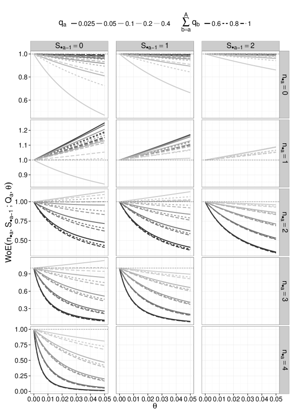
Fig. 3: $\text{\sl WoE}(n_{\bullet a},S_{\bullet a{-}1};Q_{a},\theta)$ plotted against $\theta$ for the relevant 12 combinations for a two-person DNA mixture. The horizontal black dotted lines show equal weights of evidences. The variables $n_{\bullet a}$ and $S_{\bullet a{-}1}$ refer to the margins of the allele counts and cumulative allele sums, respectively.

For a two-person DNA mixture only $15$ non-symmetric combinations exist, although for $S_{\bullet a{-}1}\geq 3$ we have that $n_{\bullet a}\leq 1$, which implies that no correlation can be observed. Therefore, only $12$ relevant combinations are shown in Fig. 3. The general picture in Fig. 3 is that$\text{\sl WoE}(n_{\bullet a},S_{\bullet a{-}1};Q_{a},\theta)<1$, except for $n_{\bullet a}=1$, where $\text{\sl WoE}(n_{\bullet a}=1,S_{\bullet a{-}1};Q_{a},\theta)\geq 1$. That is, the product of unrelated allele probabilities, $P(n_{ia}|S_{i,a{-}1})P(n_{ja}|S_{j,a{-}1})$, is smaller than the joint probability adjusting for relatedness, $P(n_{ia},n_{ja}|S_{i,a{-}1},S_{j,a{-}1})$. Hence, in the case where two or more of the same alleles are observed simultaneously, the weight of evidence is decreased. Conversely, the increased probability of homozygosity for $\theta>0$ implies that singletons, $n_{\bullet a}=1$, are less frequent, which implies an increase in the weight of evidence (Buckleton et al., 2005).

We also analysed how the ratio between $P(\bm{n}_{i})P(\bm{n}_{j})$ to $P(\bm{n}_{i},\bm{n}_{j})$ behaves. We noted that, due to the $\theta$-correction, there is an increased probability of shared alleles among DNA profiles. The behaviour is similar to that pictured in Fig. 3 since the evaluation is comprised by products of $\text{\sl WoE}(n_{\bullet a},S_{\bullet a{-}1};Q_{a},\theta)$. In Fig. 4, we see that it is possible to identify the contributions from Fig. 3. For example, the probability of observing three alleles of one type together with another allele, $(3,1)$, is the product of $\text{\sl WoE}(n_{\bullet a},S_{\bullet a{-}1};Q_{a},\theta)$ for $(n_{\bullet a},S_{\bullet a{-}1})\in\{(0,0),(1,0)$, $(3,0),(1,3),(3,1)\}$, which due to the positive correlation between alleles is dominated by $\text{\sl WoE}(n_{\bullet a}=3,S_{\bullet a{-}1}=0;Q_{a},\theta)$ and $\text{\sl WoE}(n_{\bullet a}=3,S_{\bullet a{-}1}=1;Q_{a},\theta)$.

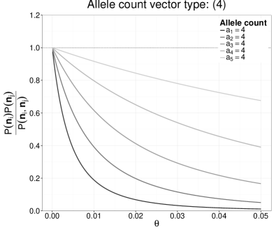
Fig. 4: The effect of $\theta$ on the match probabilities, $P(\bm{n}_{i})P(\bm{n}_{j})/P(\bm{n}_{i},\bm{n}_{j})$, for the possible profile combinations for a two-person DNA mixture with shared alleles. The underlying allele distribution is $\bm{q}=(0.025,0.05,0.1,0.2,0.4)$, where the remaining probability mass of $0.225$ is assigned to a “rest class”.

Furthermore, the legend in Fig. 4 only specifies the alleles that were observed more than once because the ratio of $P(\bm{n}_{i})P(\bm{n}_{j})$ to $P(\bm{n}_{i},\bm{n}_{j})$ for alleles observed only once cancel out. Therefore, the ratio is simplified to a function of $\theta$, which is independent of the allelic distribution. For example, in the upper left panel of Fig. 4 (dark grey curve), the ratio is the same for all vectors $\{(2,1,1,0,0,0),(2,1,0,1,0,0),\dots,$ $(2,0,0,0,1,1)\}$, i.e. all combinations with $a_{1}$ observed twice give the same ratio.

6 Conclusion

We have derived a multivariate generalisation of the Dirichlet-multinomial distribution for an application in forensic genetics. The conditional distribution over the cell counts of the multivariate Dirichlet-multinomial (MDM) distribution also follows a MDM distribution. Furthermore, the conditional distributions over vectors follow an extended hypergeometric distribution.

We have demonstrated how to incorporate the $\theta$-correction into the computational framework of the DNAmixtures package (Graversen, 2014) and exemplified how the adjustment for positive correlation between alleles caused by population stratification affects the weight of evidence.

Appendix A Generalised factorial moments of MDM

In this section, we derive the generalised factorial moments of the MDM distribution. The generalised factorial moments are useful for count data as it allows relatively simple expressions for most of the distributions’ moments. The generalised factorial moments can be considered a transformation, $f$, where we use that $\mathbb{E}\{f(\bm{n})\}=\sum_{\bm{n}\in\mathcal{N}}f(\bm{n})P(n)$.

More specifically, $f(\bm{n})=\prod_{i=1}^{I}\prod_{a=1}^{A}n_{ia}^{(r_{ia})}$, where $a^{(b)}=a!/(a-b)!$ and $r_{ia}\in\{0,\dots,n_{ia}\}$, is a vector of constants. Hence, if we want to compute $\mathbb{E}(n_{ia})$, we set $r_{ia}=1$ and all other to zero.

First, we use that conditioned on $\bm{q}$, the distribution of $\bm{n}$ is found by products of independent multinomial distributions:

$$\mathbb{E}\left\{\prod_{i=1}^{I}\prod_{a=1}^{A}n_{ia}^{(r_{ia})}\bigg{|}\bm{q}\right\} =\sum_{\bm{n}\in\mathcal{N}}\prod_{i=1}^{I}n_{i\bullet}!\prod_{a=1}^{A}\frac{n_{ia}^{(r_{ia})}}{n_{ia}!}q_{a}^{n_{ia}}$$

$$=\sum_{\bm{n}\in\mathcal{N}}\prod_{i=1}^{I}\frac{n_{i\bullet}!}{(n_{i\bullet}-r_{i\bullet})!}{n_{i\bullet}-r_{i\bullet}\choose\bm{n}_{i}-\bm{r}_{i}}\prod_{a=1}^{A}q_{a}^{n_{ia}-r_{ia}}q_{a}^{r_{ia}}$$

$$=\left\{\prod_{i=1}^{I}\frac{n_{i\bullet}!}{(n_{i\bullet}-r_{i\bullet})!}\right\}\prod_{a=1}^{A}q_{a}^{r_{\bullet a}},$$

where we moved terms constant over $\mathcal{N}=\{\bm{n}:\sum_{a}n_{ia}=n_{i\bullet}\}$ outside the sum and identified the remaining terms as being the product of independent multinomial distributions for $\bm{n}-\bm{r}$, which by definition sum to unity.

Secondly, we marginalise over $\bm{q}$ in order to obtain the generalised factorial moments for the multivariate Dirichlet-multinomial distribution

$$\mathbb{E}\left\{\prod_{i=1}^{I}\prod_{a=1}^{A}n_{ia}^{(r_{ia})}\right\} =\left\{\prod_{i=1}^{I}\frac{n_{i\bullet}!}{(n_{i\bullet}-r_{i\bullet})!}\right\}\frac{\Gamma(\alpha_{\bullet})}{\prod_{a=1}^{A}\Gamma(\alpha_{a})}\int\prod_{a=1}^{A}q_{a}^{r_{\bullet a}+\alpha_{a}-1}\,\text{d}\bm{q}$$

$$=\left\{\prod_{i=1}^{I}\frac{n_{i\bullet}!}{(n_{i\bullet}-r_{i\bullet})!}\right\}\frac{\Gamma(\alpha_{\bullet})}{\Gamma(\alpha_{\bullet}+r_{\bullet\bullet})}\prod_{a=1}^{A}\frac{\Gamma(\alpha_{a}+r_{\bullet a})}{\Gamma(\alpha_{a})}.$$

For the remaining terms, we see that the ratios of gamma functions involve $\Gamma(\beta+t)$ and $\Gamma(\beta)$. For $t>0$, the gamma function satisfies

$$\frac{\Gamma(\beta+t)}{\Gamma(\beta)}=\prod_{k=0}^{t-1}(\beta+k).$$

Hence, the expression for $\mathbb{E}(\bm{n}^{(\bm{r})})$ may be simplified to

$$\mathbb{E}\left(\bm{n}^{(\bm{r})}\right)=\mathbb{E}\left\{\prod_{i=1}^{I}\prod_{a=1}^{A}n_{ia}^{(r_{ia})}\right\}=\left\{\prod\limits_{i=1}^{I}\frac{n_{i\bullet}!}{(n_{i\bullet}-r_{i\bullet})!}\right\}\dfrac{\prod\limits_{a=1}^{A}\prod\limits_{k=0}^{r_{\bullet a}{-}1}(\alpha_{a}+k)}{\prod\limits_{k=0}^{r_{\bullet\bullet}{-}1}(\alpha_{\bullet}+k)}.$$

References

- Balding and Nichols (1994) Balding, D. J. and R. A. Nichols (1994). DNA profile match probability calculation: how to allow for population stratification, relatedness, database selection and single bands. Forensic Sci Int 64, 125–140.
- Buckleton et al. (2005) Buckleton, J. S., J. M. Curran, and S. J. Walsh (2005). How reliable is the sub-population model in DNA testimony? Forensic Sci Int 157, 144–148.
- Cowell et al. (2015) Cowell, R. G., T. Graversen, S. L. Lauritzen, and J. Mortera (2015). Analysis of Forensic DNA Mixtures with Artefacts. J R Stat Soc Ser C Appl Stat 64(1), 1–32.
- Curran et al. (2002) Curran, J. M., J. S. Buckleton, C. M. Triggs, and B. S. Weir (2002). Assessing uncertainty in DNA evidence caused by sampling effects. Sci Justice 42(1), 29–37.
- Curran et al. (1999) Curran, J. M., C. M. Triggs, J. Buckleton, and B. S. Weir (1999). Interpreting DNA mixtures in structured populations. J Forensic Sci 44(5), 987–995.
- Evett et al. (1991) Evett, I. W., C. Buffery, G. Willott, and D. Stoney (1991). A guide to interpreting single locus profiles of DNA mixtures in forensic cases. Journal of the Forensic Science Society 31(1), 41–47.
- Graversen (2014) Graversen, T. (2014). DNAmixtures: Statistical Inference for Mixed Traces of DNA. R package version 0.1-3.
- Graversen and Lauritzen (2014) Graversen, T. and S. Lauritzen (2014). Computational aspects of DNA mixture analysis. Stat Comput, 1–15. In Press.
- Green and Mortera (2009) Green, P. J. and J. Mortera (2009). Sensitivity of inferences in forensic genetics to assumptions about founding genes. Ann Appl Stat 3(2), 731–763.
- Halton (1969) Halton, J. H. (1969). A rigorous derivation of the exact contingency formula. Proc Camb Phil Soc 65(2), 527–530.
- Johnson et al. (1997) Johnson, N. L., S. Kotz, and N. Balakrishnan (1997). Discrete Multivariate Distributions. Wiley.
- Mosimann (1962) Mosimann, J. E. (1962). On the compound multinomial distribution, the multivariate -distribution, and correlations among proportions. Biometrika 49(1-2), 65–82.
- Nichols and Balding (1991) Nichols, R. A. and D. J. Balding (1991). Effects of population structure on DNA fingerprint analysis in forensic science. Heredity 66, 297–302.
- Patefield (1981) Patefield, W. M. (1981). Algorithm AS159. An efficient method of generating tables with given row and column totals. Applied Statistics 30, 91–97.
- Tvedebrink (2010) Tvedebrink, T. (2010). Overdispersion in allelic counts and -correction in forensic genetics. Theor Popul Biol 78(3), 200–210.