Disjoining Pressure and the Film-Height-Dependent Surface Tension of Thin Liquid Films: New Insight from Capillary Wave Fluctuations

Abstract

In this paper we review simulation and experimental studies of thermal capillary wave fluctuations as an ideal means for probing the underlying disjoining pressure and surface tensions, and more generally, fine details of the Interfacial Hamiltonian Model. We discuss recent simulation results that reveal a film–height–dependent surface tension not accounted for in the classical Interfacial Hamiltonian Model. We show how this observation may be explained bottom–up from sound principles of statistical thermodynamics and discuss some of its implications.

20131104

1 Introduction

As materials science and nanotechnology improve our ability to produce devices of smaller and smaller size down to the nanoscale, the importance of interfacial phenomena becomes yet more relevant [1].

Indeed, current methods allow us to prepare intricate devices, which feature grooves, channels and containers, offering the possibility to process minute amount of liquids in a controlled manner [2, 3, 4].

Obviously, the operation of such devices requires detailed understanding of the fluid’s behavior, and the size to surface ratio of the condensates that result makes the role of surface interactions a key issue [5]. At sub–micrometer length scales, however, the classical surface thermodynamics of Young and Laplace may well not be sufficient [6]. The precise nature of the fluid–substrate interactions becomes important, and it is no longer possible to lump all such effects into a macroscopic contact angle. Attempts to extend the validity of the classical thermodynamic approach are based on the addition of line tension effects [7, 8, 9, 10], and provide encouraging results [11, 12, 6, 13, 14, 15]. However, this concept meets difficulties and controversies [16, 17, 18, 19], and is difficult to extend beyond the study of sessile droplets.

A well known route to study adsorption phenomena at such length scale refines the level of coarse–graining one step below, by describing the properties of the adsorbed liquid in terms of a film height, $\ell$. This provides a means to incorporate surface forces in a detailed manner [20, 16, 21, 22, 23], using the celebrated Derjaguin’s concept of disjoining pressure, $\Pi(\ell)$ [24, 25], or, alternatively, the corresponding interface potential $g(\ell)$ [26, 27].

Our understanding of wetting phenomena owes a great deal to such concept. More interestingly, however, the interface potential also offers the possibility to study the properties of inhomogeneous films, by means of a simple phenomenological extension, known as the Interfacial Hamiltonian Model (IHM). In this model, one defines a film profile, $\ell(\mathbf{x})$, dictating the film height on each point of the underlying plane. Each infinitesimal surface area element $d\mathbf{x}$, bares a free energy $g(\ell(\mathbf{x}))$ dictated by the film height at that point. However, since the film is inhomogeneous, an additional contribution accounting for the increase of the liquid–vapor interfacial area is required. Considering both contributions, and integrating over the whole plane of the substrate, one arrives at [16, 23]:

$$H[\ell(\mathbf{x})]=\int\left\{g(\ell)+\gamma_{\infty}(\sqrt{1+(\nabla\ell)^{2}}-1)\right\}d\mathbf{x}$$ (1)

where $\gamma_{\infty}$ is the liquid–vapor surface tension, while the label ”$\infty$” as a subindex emphasizes the fact that, for whatever film height, we refer to the surface tension of a film away from the influence of the disjoining pressure. i.e., the liquid–vapor surface tension. Since equilibrium film profiles are extrema of $H[\ell]$, it may be readily found that the IHM is essentially equivalent to the augmented Young–Laplace equation that is familiar in surface science [20, 16, 21, 22, 23].

The importance of Eq. (1) should not be overlooked, as it forms the basis for most theoretical accounts of surface phenomena, including, the study of capillary waves [28], renormalization group analysis of wetting phenomena [29], the prediction of droplet profiles [30], the measure of line tensions [31], the structure of adsorbed films on patterned substrates [32], and the dynamics of dewetting [33].

Despite its theoretical importance, it has been argued for already some time that the IHM cannot be derived bottom–up from a microscopic Hamiltonian of finer coarse–graining level [34]. This issue has received a great deal of attention in the context of adsorbed fluids subject to a short–range wall–fluid potential. This system exhibits a critical wetting transition, the liquid film can grow almost unbound, and the interfacial fluctuations become increasingly large [35]. As a result, the wetting behavior cannot be accounted properly by the mean field interface potential, $g(\ell)$, but rather, must be described by suitable renormalization of Eq. (1). Conflicting results of the theoretical analysis [29] with simulations [36], motivated a critical assessment on the foundation of IHM [37, 38, 39]. Fisher and Jin attempted to derive Eq. (1) using a Landau–Ginzburg–Wilson Hamiltonian, and argued that this is possible provided one replaces $\gamma_{\infty}$ by a film–thick dependent surface tension, $\gamma(\ell)$ which approaches $\gamma_{\infty}$ exponentially fast [37, 38]. However, further studies by Parry and collaborators have shown that IHM is actually a nonlocal functional which does generally not satisfy Eq. (1), except for some simple situations [39, 40].

Unfortunately, these studies are limited to the special case of short–range forces, which are only found in nature under exceptional circumstances, as they correspond to an effectively vanishing Hamaker constant [41, 42]. The more relevant case of fluids in the presence of van der Waals interactions, has apparently received much less attention [43, 44, 45], possibly because the long–range interactions inhibit fluctuations and do not warrant a renormalization analysis.

However, the problem remains an issue of great importance for the study of inhomogeneous films under confinement–condensed sessile drops, fluids adsorbed in grooves, and other condensed structures–irrespective of the presence of critical fluctuations!

In fact, thin adsorbed films subject to van der Waals forces still exhibit thermal surface fluctuations of amplitudes as large as the $mm$ scale that are known under the name of capillary waves [28, 46]. The study of this, less exquisite fluctuations actually can convey not only a great deal of information on the underlying surface forces [47, 48, 49], but is actually also a stringent test of the Interface Hamiltonian Model itself [45, 50, 51].

In this paper, we will review studies of the capillary wave fluctuations of adsorbed films performed over the last years, and describe recent findings which shed some light on the conjectured dependence of the surface tension with film height [52, 53, 45].

In the next section, we will give an overview of well known liquid–state theories for the description of density profiles of planar adsorbed films. Since these theories are of mean field type, they lead to structural properties which are intrinsic to the fluid–substrate pair considered, and do not depend on other external considerations such as the system size. In section 3, we give a brief overview of classical capillary wave theory and show how it allows to probe the interfacial structure of films as well as to validate the Interfacial Hamiltonian Model. We illustrate the classical predictions with a number of experiments and computer studies, and show how the capillary fluctuations renormalize the intrinsic density profiles, which actually become system size dependent and are therefore not intrinsic properties of the fluid–substrate pair. In Section 4 we describe computer simulation techniques for the study of capillary wave fluctuations, and discuss how very recent simulation evidence has gathered that calls for an improved interfacial Hamiltonian model. This problem is reviewed in section 5, where the results of section 2 are applied in order to derive an interfacial Hamiltonian bottom–up, for fluid films subject to surface forces decaying well beyond the bulk liquid correlation length, as is usually the case in real systems exhibiting dispersion forces. Finally, section 6 summarizes the outcome of the study and discusses some of its implications.

2 Liquid state theory of adsorbed fluids

In modern liquid–state theory, the study of interfaces is formulated in terms of free energy functionals of the number density, $\rho(\mathbf{r})$ [54]. Paralleling the expression of the Helmholtz free energy of a volumetric system, i.e., $F=Nk_{B}T(\ln\Lambda^{3}\rho-1)+F_{\rm ex}$, which includes ideal and excess contributions, one writes, for the inhomogeneous system, the following density functional:

$$F[\rho(\mathbf{r})]=k_{B}T\int\rho(\mathbf{r})\left(\ln\Lambda^{3}\rho(\mathbf{r})-1\right)d\mathbf{r}+F_{\rm ex}[\rho(\mathbf{r})]$$ (2)

where $N$ is the number of molecules, $k_{B}$ is Boltzmann’s constant, $T$ is the absolute temperature and $\Lambda$ is the thermal de Broglie wavelength, while $F_{\rm ex}$ is a highly non–trivial functional incorporating all unknown multibody correlations.

In practice, it is more convenient to relax the constraint over fixed number of particles that is appropriate for Helmholtz free energies, and consider a system with fixed bulk chemical potential $\mu_{\infty}$. This is achieved by introducing the grand free energy $\Omega$, a new functional of the density which can be obtained from $F$ by Legendre transformation, $F-\mu_{\infty}N\to\Omega$.

$$\Omega[\rho(\mathbf{r})]=F[\rho(\mathbf{r})]+\int\rho(\mathbf{r})(V(\mathbf{r})-\mu_{\infty})d\mathbf{r}$$ (3)

where we have also included here $V(\mathbf{r})$, an external field that will usually be the responsible for creating the inhomogeneity under study. For an adsorbed fluid, $V(\mathbf{r})$ may be the van der Waals long range potential mimicking the interactions with the substrate; for a free fluid–fluid interface it may be the potential energy felt by an atom due to gravity.

Within mean–field theory, we expect that the equilibrium average profile is that which minimizes $\Omega$, subject to the constraints of constant volume, temperature and chemical potential:

$$\frac{\delta\Omega}{\delta\rho(\mathbf{r})}=0$$ (4)

Performing the functional minimization of Eq. (3), together with Eq. (2), we obtain:

$$\rho(\mathbf{r})=\rho_{\infty}\exp\{-\beta V(\mathbf{r})+C^{(1)}(\mathbf{r})+\beta\mu_{\rm ex}\}$$ (5)

where $\beta=1/k_{B}T$, $\rho_{\infty}$ is the bulk density at the imposed chemical potential, $\mu_{\rm ex}$ is the corresponding excess chemical potential and $C^{(1)}(\mathbf{r})$ is the so called singlet direct correlation function:

$$C^{(1)}(\mathbf{r})=-\frac{\delta\beta F_{\rm ex}[\rho(\mathbf{r})]}{\delta\rho(\mathbf{r})}$$ (6)

The above equation is the first member of a hierarchy defining direct correlation functions of arbitrary order [46, 55]. The next member of the series provides the direct pair correlation function as:

$$C^{(2)}(\mathbf{r},\mathbf{r}^{{}^{\prime}})=\frac{\delta C^{(1)}(\mathbf{r};[\rho])}{\delta\rho(\mathbf{r}^{{}^{\prime}})}$$ (7)

By integrating the above equation from some density reference profile, $\rho_{0}(\mathbf{r})$, to the actual density profile, we obtain:

$$C^{(1)}(\mathbf{r};[\rho])=C^{(1)}(\mathbf{r};[\rho_{0}])+\int\int C^{(2)}(\mathbf{r},\mathbf{r}^{{}^{\prime}};[\rho])\,\delta\rho\,d\mathbf{r}^{{}^{\prime}}$$ (8)

This equation is formally exact but of little use, since we ignore the exact form of both $C^{(1)}(\mathbf{r};[\rho_{0}])$ and $C^{(2)}(\mathbf{r},\mathbf{r}^{{}^{\prime}};[\rho])$. We can however, consider a flat reference profile, such that $\rho_{0}(\mathbf{r})=\rho_{\infty}$, and further assume that the direct pair correlation function does not depend significantly on deviations of $\rho(\mathbf{r})$ away from the reference density $\rho_{0}$. With these approximations we obtain an asymptotic density expansion:

$$C^{(1)}(\mathbf{r};[\rho])=C^{(1)}(\rho_{\infty})+\int\Delta\rho(\mathbf{r}^{{}^{\prime}})\,C^{(2)}(\mathbf{r},\mathbf{r}^{{}^{\prime}};\rho_{\infty})d\mathbf{r}^{{}^{\prime}}$$ (9)

where $\Delta\rho(\mathbf{r})=\rho(\mathbf{r})-\rho_{\infty}$, while the unknown singlet correlation function is now expressed in terms of singlet and pair correlation functions of a homogeneous fluid with asymptotic density $\rho_{\infty}$.

This is a convenient result, because much is known about the direct correlation function of bulk simple fluids [56, 57]. One could thus employ such knowledge to calculate $C^{(1)}(\mathbf{r};[\rho])$ accurately and exploit Eq. (5) and Eq. (9) to predict the density profile. Unfortunately such a program can only be carried out with heavy numerical calculations [58, 59, 60]. In order to obtain tractable expressions, it is necessary to get rid of the nonlocal integral by performing a gradient expansion of the density difference $\Delta\rho(\mathbf{r}^{{}^{\prime}})$ about $\Delta\rho(\mathbf{r})$ to second order. Considering that the bulk direct correlation function of an atomic fluid is an even function of $|\mathbf{r}^{{}^{\prime}}-\mathbf{r}|$, we find that odd terms in the expansion vanish, and get [61]:

$$C^{(1)}(\mathbf{r};[\rho])=C^{(1)}(\rho_{\infty})+\left(\frac{1}{\rho_{\infty}}-\frac{\beta}{\kappa_{\infty}\rho_{\infty}^{2}}\right)\Delta\rho(\mathbf{r})+C_{\infty}\nabla^{2}\Delta\rho(\mathbf{r})$$ (10)

where the coefficient linear in $\Delta\rho(\mathbf{r})$ is the zero order moment of the direct pair correlation function and may be related to the bulk compressibility, $\kappa_{\infty}$, via the Ornstein–Zernike equation [46]:

$$\int C^{(2)}(\mathbf{r};\rho_{\infty})d\mathbf{r}=\frac{1}{\rho_{\infty}}-\frac{\beta}{\kappa_{\infty}\rho_{\infty}^{2}}$$ (11)

and $C_{\infty}$ is the second moment of the direct pair correlation function:

$$C_{\infty}=\frac{1}{6}\int\mathbf{r}^{2}C^{(2)}(\mathbf{r};\rho_{\infty})d\mathbf{r}$$ (12)

If we now substitute Eq. (10) into Eq. (5) and linearize the exponential term, we find that $\Delta\rho(\mathbf{r})$ is determined by the following second order partial differential equation:

$$\nabla^{2}\Delta\rho(\mathbf{r})-b_{\infty}^{2}\Delta\rho(\mathbf{r})=\frac{\beta}{C_{\infty}}V(\mathbf{r})$$ (13)

where $b_{\infty}=\xi_{\infty}^{-1}$, while $\xi_{\infty}$ is the bulk correlation length, given by:

$$\xi_{\infty}^{2}=k_{B}TC_{\infty}\kappa_{\infty}\rho_{\infty}^{2}$$ (14)

Essentially, Eq. (13) corresponds to a square–gradient theory for the Helmholtz free energy functional, with a parabolic approximation for the local free energy (see below). The advantage of the systematic derivation from first principles is that a deeper insight on the nature of the square–gradient coefficient is obtained.

Unfortunately, this equation has one very important limitation that may have been overlooked: it relies on a gradient expansion of the density perturbations, $\Delta\rho(\mathbf{r})$. This implies that the coefficients of the successive derivatives are moments of the direct correlation function (e.g. as is the case of the coefficient of $\nabla^{2}\Delta\rho$, c.f. Eq. (12) ). The direct correlation function itself is known to decay as the underlying pair potential so that the higher order moments can only converge if the fluid pair potential is short range, i.e., is either truncated at a finite value or decays exponentially fast. These considerations imply that the results obtained so far are strictly valid only for short–range fluids with exponential decay of the pair interactions [54]. Later on we will discuss at length the significance of these limitations (c.f. section 2.4).

In what follows, we will exploit the above result in order to study density profiles of the liquid–vapor and wall–liquid interfaces. For such systems, the average density profile depends only on the perpendicular distance to the interface, $z$, so that the Helmholtz equation becomes a simple linear ordinary differential equation:

$$\frac{d^{2}\Delta\rho(z)}{dz^{2}}-b_{\infty}^{2}\Delta\rho(z)=\frac{\beta}{C_{\infty}}V(z)$$ (15)

Later on, we will see that the approach starting from Eq. (9) can also be extended to study oscillatory profiles of fluids adsorbed on a wall.

2.1 Liquid–Vapor Interface

Let us now consider the inhomogeneous density profile that results when a homogeneous fluid phase separates at zero field, such that $V(z)=0$. In principle, it is impossible to study a liquid–vapor interface from the result of Eq. (15). The reason is that it is essentially a local expansion about a reference bulk density, say the vapor density, and hence, cannot possibly carry any information about the liquid phase. In practice, however, one can exploit this result to study perturbations of the liquid and vapor branches of the density profile independently and get a full liquid–vapor density profile by matching the separate pieces. This approximation constitutes the double–parabola model of interfaces [37]. The name stems from the parabolic approximation about the vapor and liquid minima of the local Helmholtz free energy that is implied. This becomes more clear if we consider the well known square–gradient functional of inhomogeneous fluids [62]:

$$\beta F[\rho(\mathbf{r})]=\int\left\{\beta f(\rho(\mathbf{r}))+\frac{1}{2}\,C_{\infty}\left[\nabla\rho(\mathbf{r})\right]^{2}\right\}d\mathbf{r}$$ (16)

where the local free energy is given by $f(\rho)=\rho\mu(\rho)-p(\rho)$ and $p(\rho)$ is the pressure. Substitution of this square–gradient functional into Eq. (3), followed by extremalisation, yields:

$$C_{\infty}\nabla^{2}\Delta\rho(\mathbf{r})-\beta[\mu(\rho)-\mu_{\infty}]=\beta V(\mathbf{r})$$ (17)

This equation cannot be solved analytically for a general isotherm $\mu(\rho)$, but can be related to Eq. (15) upon linearisation of the chemical potential about the coexistence value, whereby $\mu(\rho)-\mu_{\infty}$ becomes simply $(\rho-\rho_{\infty})/(\rho_{\infty}^{2}\kappa_{\infty})$, and Eq. (17) then immediately transforms into Eq. (13). Linearising the isotherm about the coexistence liquid and vapor densities, and solving for each branch separately constitutes the double parabola approximation. The linearised chemical potential isotherm results from derivation of a parabolic Helmholtz free energy centered about the coexistence density, thus explaining the name of the model (c.f. Fig.1).

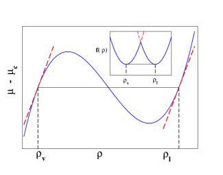
Figure 1: Sketch of the double parabola approximation for the chemical potential isotherm. Full lines depict the full van der Waals loop in the $\mu-\rho$ plane, and the dashed lines illustrate the linearisation that is performed about the coexistence vapor and liquid densities. The linear extrapolation of the equation of state results from differentiation of a double parabolic model for the free energy (inset).

Consider the liquid–vapor interface is located at $z=\ell$, with the asymptotic liquid phase of density $\rho_{l}$ to the left ($z<\ell$), and the asymptotic vapor phase of density $\rho_{v}$ to the right of $\ell$ ($z>\ell$). With this boundary conditions so defined, we can solve Eq. (15) for each branch separately, obtaining a piecewise solution of the form:

$$\rho_{\rm lv}(z)=\left\{\begin{array}[]{cc}\rho_{l}+A_{l}e^{b_{l}z}&z<\ell\\ \\ \rho_{v}+A_{v}e^{-b_{v}z}&z>\ell\end{array}\right.$$ (18)

In order to solve for the integration constants, $A_{l}$ and $A_{v}$, two possible extra boundary conditions come to mind. The first is the crossing criterion [37, 38], which requires the continuity of the piecewise function, Eq. (18) at $z=\ell$, and defines $\ell$ such that the density at that point is precisely some chosen value, say, $\rho_{1/2}$, which is, most naturally, but not necessarily equal to the average $(\rho_{l}+\rho_{v})/2$:

$$\left\{\begin{array}[]{ccc}\lim_{z\to\ell^{-}}\rho_{\rm lv}(z)&=&\lim_{z\to\ell^{+}}\rho_{\rm lv}(z)\\ \\ \rho_{\rm lv}(z=\ell)&=&\rho_{1/2}\\ \end{array}\right.$$ (19)

The crossing criterion provides a set of two linear equations that can be easily solved for $A_{l}$ and $A_{v}$, and leads to the following result for the piecewise liquid–vapor density profile [37]:

$$\rho_{\rm lv}(z)=\left\{\begin{array}[]{cc}\rho_{l}+(\rho_{1/2}-\rho_{l})e^{b_{l}(z-\ell)}&z<\ell\\ \\ \rho_{v}+(\rho_{1/2}-\rho_{v})e^{-b_{v}(z-\ell)}&z>\ell\end{array}\right.$$ (20)

This model has proved very convenient, as it provides analytic results for the density profiles and free energies of interfaces perturbed by capillary waves [37, 38, 63, 39, 43, 44]. Although we have cast it here in a form that accounts for the asymmetry of the vapor and liquid phases, most usually one assumes a symmetric fluid, hence $b_{l}=b_{v}$.

As just mentioned, the crossing criterion would seem to account for the asymmetry of the vapor and liquid phases. However, the first derivative of the density profile becomes discontinuous whenever $b_{l}\neq b_{v}$. In order to remedy this problem, it is possible to introduce a smooth matching criterion by requiring continuity of both the density and its first derivative at $z=\ell$ i.e.,

$$\left\{\begin{array}[]{ccc}\lim_{z\to\ell^{-}}\rho_{\rm lv}(z)=\lim_{z\to\ell^{+}}\rho_{\rm lv}(z)\\ \\ \lim_{z\to\ell^{-}}\frac{d\rho_{\rm lv}(z)}{dz}=\lim_{z\to\ell^{+}}\frac{d\rho_{\rm lv}(z)}{dz}\\ \end{array}\right.$$ (21)

Solving the matching conditions for $A_{l}$ and $A_{v}$, now yields:

$$\rho_{\rm lv}(z)=\left\{\begin{array}[]{cc}\rho_{l}-\frac{b_{v}}{b_{v}+b_{l}}(\rho_{l}-\rho_{v})e^{b_{l}(z-\ell)}&z<\ell\\ \\ \rho_{v}+\frac{b_{l}}{b_{v}+b_{l}}(\rho_{l}-\rho_{v})e^{-b_{v}(z-\ell)}&z>\ell\end{array}\right.$$ (22)

Despite its simplicity, the model incorporates naturally the asymmetry of the liquid and vapor phases, remains continuous up to the first derivative, and is able to provide semi–quantitative results for the density profiles and surface tensions of simple fluids [64]. Furthermore, the model may be extended to study spherical interfaces, also providing analytical results for density profiles and nucleation energies [65, 66, 67, 64].

Such analytical results cannot be obtained otherwise except for very few selected toy models (e.g.: [68, 46]).

2.2 Wall–liquid Interface

Simple atomic liquids close to a rigid substrate exhibit a stratified structure that results from packing effects of the dense phase. Such behavior is well known from both theoretical calculations and atomic force microscopy experiments [69, 70, 71, 72, 73, 74, 75].

The model for fluid interfaces discussed in the previous section would seem not adequate to describe this behavior, since it may be interpreted as a plain squared gradient theory solved piecewise. With this perspective, one can only expect it to provide adequate results for smoothly varying density perturbations. However, it is possible to exploit the explicit connection with the direct pair correlation function embodied in Eq. (10)–Eq. (12) in order to provide a qualitative explanation for the oscillatory behavior found in experiments. First, notice that the coefficients of Eq. (10) are actually zero and second moments of the direct correlation function. Whence, they can also be interpreted as their zero wave–vector Fourier transforms. Taking this into account, it becomes apparent that the theory formulated previously is adequate to study perturbations of long wavelength only.

Molecular fluids at high density usually exhibit a maximum of the structure factor, $S(k)$ at finite wave–vector, $k_{\rm o}$. Such a maximum is indicative of strong structural correlations of wavelength $\lambda=2\pi/k_{o}$. Accordingly, it seems natural to particularize the study of density fluctuations to the form $\Delta\rho(\mathbf{r})=a(\mathbf{r})e^{\pm i{\bf k}_{\rm o}\cdot\mathbf{r}}$, where the second factor of the right hand side now imposes correlations of the adequate wavelength, while the first factor, $a(\mathbf{r})$ describes the corresponding amplitudes. In the regime of linear response, it is these amplitudes that should vary smoothly, rather than the whole density wave $\Delta\rho(\mathbf{r})$. Therefore, one can perform a gradient expansion of $a(\mathbf{r}^{{}^{\prime}})$ about $a(\mathbf{r})$, similar to that performed previously for $\Delta\rho(\mathbf{r}^{{}^{\prime}})$ about $\Delta\rho(\mathbf{r})$. After insertion of the expansion into Eq. (9), followed by substitution in the linearized form of Eq. (5), we obtain a Helmholtz equation for the amplitudes rather than for the densities [76]:

$$\nabla^{2}a(\mathbf{r})-b^{2}_{\rm o}a(\mathbf{r})=0$$ (23)

where now, the coefficient $b_{\rm o}=1/\xi_{o}$, while $\xi_{o}^{2}=k_{B}TC_{o}\kappa_{o}\rho_{\infty}^{2}$ is given in terms of a generalized wave–vector dependent compressibility (c.f. Eq. (11)):

$$\int C^{(2)}(\mathbf{r})e^{i{\bf k}_{o}\cdot\mathbf{r}}d\mathbf{r}=\frac{1}{\rho_{\infty}}-\frac{\beta}{\kappa_{o}\rho_{\infty}^{2}}$$ (24)

and $C_{o}$ is a Fourier transform of the direct pair correlation function’s second moment:

$$C_{o}=\frac{1}{6}\int\mathbf{r}^{2}C^{(2)}(\mathbf{r})e^{i{\bf k}_{o}\cdot\mathbf{r}}d\mathbf{r}$$ (25)

Let us consider the solution of Eq. (23) for the simple case of a “contact” potential of delta–Dirac form whose only role is to impose a boundary condition for the density of the film precisely at the wall contact, $z=d_{w}$. The solution of this equation proceeds then exactly as for Eq. (13), and yields for the wall–liquid density profile the following result:

$$\rho_{wl}(z)=\rho_{l}(1+A_{w}cos(k_{\rm o}z+\theta_{w})e^{-b_{\rm o}z})$$ (26)

where $A_{w}$ is the amplitude of the density wave imposed by the contact wall potential and $\theta_{w}$ is the phase. An interesting point which is worth stressing is that both $k_{o}$ and $b_{\rm o}$ are structural properties of the bulk liquid. Only the amplitude $A_{w}$ and the phase $\theta_{w}$ actually depend on details of the wall–fluid interactions.

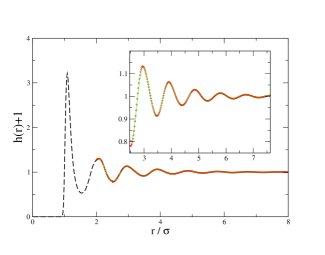
Figure 2: Bulk total correlation function of a Lennard–Jones fluid close to its triple point. The dashed line corresponds to simulation results, and the full line is the result of a fit to $rh(r)=A_{o}cos(k_{o}r+\theta_{f})exp(-b_{o}r)$ (c.f. Eq. (29)). Symbols indicate simulation results in the range where the fit is performed. The inset shows a detailed view (c.f. Ref.[45, 53] and Sec. 4.3 for further details on the model and simulations).

The result shown here is actually a particular case of a more general theory relating the density profile of an adsorbed fluid with its bulk structural properties [77, 78, 79]. A study of the Ornstein–Zernike equation shows that, quite generally, the total pair correlation function, $h(r)$ of an isotropic fluid is given by:

$$rh(r)=\sum_{j}A_{j}e^{ik_{j}r}$$ (27)

where the sum runs over the poles of the structure factor, i.e., the set of complex wave–vectors satisfying $\rho C^{(2)}(k_{j})-1=0$ [77]. If, on the other hand, one considers the wall–liquid total correlation function, $h_{\rm wl}(z)$, the Ornstein–Zernike equation dictates rather that:

$$h_{\rm wl}(z)=\sum_{j}B_{j}e^{ik_{j}z}$$ (28)

where the sum runs over exactly the same set of wave–vectors than before, and only the coefficients $B_{j}$ are actually dependent on the wall–fluid substrate. A lucky coincidence is that only the first few leading order terms in this expansion are necessary to obtain a very precise description of the fluid structure. Particularly, for fluids with short range forces, a formal study reveals that the two longest range wave–vectors, $k_{j}$ are, i) a purely imaginary pole, leading to pure exponential decay, and ii) a conjugate–pair of complex poles, leading to damped oscillatory decay.

Therefore, the long range decay of the bulk pair correlation function is of the form:

$$rh(r)=A_{e}e^{-b_{e}r}+A_{o}cos(k_{o}r+\theta_{f})e^{-b_{o}r}$$ (29)

while that of the wall–liquid pair correlation function is given by:

$$h_{wl}(z)=B_{e}e^{-b_{e}z}+B_{o}cos(k_{o}z+\theta_{w})e^{-b_{o}z}$$ (30)

For high temperature, $b_{o}>b_{e}$, and the long–range decay is purely monotonic. At lower temperatures, however, the contrary holds and the long–range decay becomes damped–oscillatory. These two regimes are separated in the temperature–density plane of the phase diagram as a line $T_{\rm fw}(\rho)$ that is known as the Fisher–Widom line [80]. Actually, at temperatures close to the triple–point, the monotonic contribution is of such short range that only one damped–oscillatory term serves to precisely describe the pair correlation function beyond the first maximum.

The accuracy of this prediction has been assessed in Density Functional Studies [78], as well as experimentally [75, 81]. As an example, Fig.2 shows the simulated bulk total correlation function of a Lennard–Jones model of Argon close to its triple point. Clearly, a strong oscillatory behavior is visible, but all of the correlation function may be accurately described beyond two molecular diameters, $\sigma$, with a single damped oscillatory term. Simulating now liquid Argon at the same thermodynamic conditions but adsorbed to an attracting wall, provides the density profile given in Fig.3. Using only the damped oscillatory term of Eq. (30), with $k_{o}$ and $b_{o}$ from the fit to the bulk correlation function, and only the amplitude $B_{o}$ and phase $\theta_{w}$ as new fitting parameters, provides again an excellent description beyond two molecular diameters. Such a particularly simple behavior is a result of the low temperatures considered. At higher temperature, at least the leading order purely exponential contribution needs to be added.

It should be stressed, however, that Eq. (29)–Eq. (30) are only appropriate for fluids with short–range forces. This is almost always the case in simulation studies, since the dispersion tail $r^{-6}$ is in practice, truncated beyond some reasonable value. Taking van der Waals contributions for the fluid–fluid pair potential into account makes the formal analysis become far more difficult, but it is expected that the gross features described here will still hold [79]. For example, it is well known that the tails of the liquid–vapor density profile of a long–range fluid with interactions of the form $r^{-6}$ will decay as $z^{-3}$, instead of exponentially [61], but these finer details need not concern us here. Surprisingly, even van der Waals wall–liquid interactions of range $z^{-3}$ actually have a negligible effect on the structure of the density profile. This can be assessed by exploiting yet once more Eq. (13), as a means to measure the density fluctuation $\Delta\rho(z)$ that results from a long range perturbation $V(z)\propto z^{-3}$. Noticing that Eq. (18) already provides the homogeneous solution for Eq. (15), we seek for a particular solution of the form:

$$\Delta\rho(z)=\sum_{i=0}^{\infty}a_{i}\,V^{(i)}(z)$$ (31)

where $a_{i}$ are undetermined coefficients and $V^{(i)}$ stands for the $i$th derivative of $V(z)$. Note that the particular solution suggested is actually valid for algebraically decaying potentials. For an exponential decay, the first term of the series would suffice. Now, substitution of the trial form into Eq. (15), followed by identification of the coefficients, yields:

$$\Delta\rho(z)=-\frac{\beta}{C_{\infty}b_{\infty}^{2}}\sum_{i=0}^{\infty}\left(\frac{1}{b_{\infty}^{2}}\right)^{i}V(z)^{(2i)}$$ (32)

Considering that, by virtue of Eq. (11), the prefactor is essentially dictated by the fluids susceptibility, $d\rho/d\mu$, if follows that the density profile of incompressible fluids will be hardly affected by the long–range substrate potential. In order to grasp more transparently the significance of the above equation, it is now convenient to perform a resummation of the linearized result. Employing Eq. (32) in order to evaluate Eq. (10), followed by substitution of the result into Eq. (5) and neglect of the higher order terms, yields the following more familiar equation:

$$\rho(z)=\rho_{\infty}e^{-\beta\kappa_{\rm rel}V(z)}$$ (33)

where $\kappa_{\rm rel}=\kappa_{\infty}/\kappa_{ig}$ is the ratio of bulk to ideal gas compressibilities. This result is thus essentially a generalization of the barometric law for dense fluids. For small densities, $\kappa_{\rm rel}=1$, and Eq. (33) becomes the ideal gas distribution under an external field. Close to the triple point of Argon, however, the ratio $\kappa_{\rm rel}$ is of the order $10^{-2}$, and the density profile is then hardly perturbed except for the immediate vicinity of the substrate. This form of the asymptotic behavior of the density profile can also be obtained from an analysis of the Ornstein–Zernike equation [82, 78].

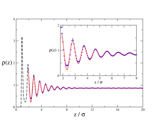
Figure 3: Density profile at the wall–liquid interface of a Lennard–Jones fluid close to its triple point. The dashed line corresponds to simulation results. The full line is the result of a fit to $B_{o}cos(k_{o}z+\theta_{w})exp(-b_{o}z)$ (c.f. Eq. (30)) with $k_{o}$ and $b_{o}$ obtained from the bulk correlation function and only $B_{o}$ and $\theta_{w}$ as fitting parameters. Symbols indicate simulation results in the range where the fit is performed. The inset shows a detailed view (c.f. Ref.[45, 53] and Sec. 4.3 for further details on the model and simulations).

2.3 Adsorbed Films

Previously, we have obtained analytic results for the density profile of a liquid–vapor and a wall–liquid interface. We are now in a good position to consider the density profile of an adsorbed film of finite thickness $\ell$, which one expects, should exhibit structural properties that are similar to those of the liquid–vapor interface in the neighborhood of $\ell$ and similar to those of the wall–liquid interface as one approaches the substrate.

In principle, one could employ the double parabola model of section 2.2 in order to obtain the full density profile of such an adsorbed film. This can be achieved by adding an extra exponential tail $A_{w}e^{-b_{l}z}$ into the trial solution for the liquid branch, and solving for the constant $A_{w}$ with a new boundary condition at the wall. This leads to a smooth density profile which may exhibit either an enhanced or depleted contact density at the wall depending on the boundary condition that is imposed [37]. If one is willing to describe the oscillations that propagate from the wall, it suffices to seek for solutions of the liquid branch where the new monotonic exponential tail is replaced with an oscillatory tail $A_{w}e^{-(b_{o}+ik_{o})z}$.

In practice, however, we find that retaining the form of the wall–liquid and liquid–vapor profiles, and superimposing the former on the latter actually works much better. In this superposition approximation, we write for the film profile:

$$\rho(z;\ell)=[1+h_{\rm wl}(z)]\,\rho_{\rm lv}(z;\ell)$$ (34)

where $h_{\rm wl}(z)$ has the form of Eq. (30), while $\rho_{\rm lv}(z;\ell)$ is the liquid–vapor density profile in the double parabola approximation, Eq. (18). The integration constants $A_{l}$ and $A_{v}$ may be readily calculated within the crossing criterion, providing the following piecewise profile for the adsorbed film:

$$\rho(z;\ell)=[1+h_{\rm wl}(z)]\times\left\{\begin{array}[]{cc}\rho_{l}+\frac{\rho_{1/2}-\rho_{l}[1+h_{\rm wl}(\ell)]}{1+h_{\rm wl}(\ell)}e^{b_{l}(z-\ell)}&z<\ell\\ \\ \rho_{v}+\frac{\rho_{1/2}-\rho_{v}[1+h_{\rm wl}(\ell)]}{1+h_{\rm wl}(\ell)}e^{-b_{v}(z-\ell)}&z>\ell\\ \end{array}\right.$$ (35)

As is the case of the crossing criterion applied to the liquid–vapor interface, the resulting profile is continuous at $z=\ell$, but its derivative is not. In principle, one could also apply the smooth matching criterion here, but the equations that result are far too lengthy.

The fact is that, already at the level of the crossing approximation, Eq. (35) predicts simulated density profiles with surprising accuracy. Figure 4 shows a series of density profiles for films of a Lennard–Jones model of Argon on an adsorbing substrate in the neighborhood of the triple point. The structural parameters for $h_{\rm wl}(z)$ are obtained from results of the wall–liquid interface described previously in Fig.3, while the inverse correlation lengths $b_{v}$ and $b_{l}$ for the double parabola model of $\rho_{lv}(z)$ are obtained from a fit to the free liquid–vapor interface. The film height for the model profile is then determined such that it matches the simulated profile exactly at $z=\ell$, which, by construction, amounts to defining $\ell$ such that the crossing criterion is met for both the model and the simulated profiles. The predicted results are compared with simulations in Fig.4, clearly showing good agreement even for films as thin as $\ell=1.9$ molecular diameters.

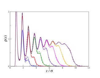
Figure 4: Density profiles of adsorbed films for the Lennard–Jones fluid close to its triple point. Full lines are simulation results for films of thickness $\ell$ (from left to right) 1.9, 3.0, 4.1, 5.3, 6.5, 7.3 and 8.5 molecular diameters, $\sigma$. Dashed lines are predictions from the superposition model, Eq. (35). Note that the discontinuity in the first derivative of the density profile is hardly visible (results adapted from Ref.[45, 83] correspond to the same model and temperature as the two preceding figures).

2.4 Short range versus long range forces

In this chapter, we have seen how Density Functional Theory may provide accurate and analytic results for density profiles of inhomogeneous fluids. It is also pleasing to see that all such results, whether the shape of the liquid–vapor interface, the density profile of a liquid in the neighborhood of a substrate, or the structure of an adsorbed liquid film, are obtained within a consistent and unified framework based on a single apparently general result, namely, Eq. (9).

The density profiles for adsorbed films that are provided via Eq. (35), may be replaced back into the underlying density functional in order to obtain accurate estimates of the film’s free energy. Particularly, one can obtain from the free energy functional the interface potential, i.e., the free energy of an adsorbed film of height $\ell$, measured relative to the free energy of an infinitely thick film. To leading order, this is given by [71, 78]:

$$g_{\rm sr}(\ell)=-A_{1}\cos(k_{o}\ell+\theta_{w})e^{-b_{o}\ell}+A_{2}e^{-2b_{o}\ell}$$ (36)

where $A_{1}$ and $A_{2}$ are positive constants. Unfortunately, this model applies for strictly short–range forces. This also includes the wall–fluid interactions, which are considered in this expression as a contact potential of virtually zero range.

In practice, however, most fluids are subject to power–law interactions that will decay as $r^{-6}$ or even slower [5]. What is the status of our results then? Simple analytical expressions for long–range fluids are extremely difficult to obtain already for van der Waals interactions. Fortunately, one can still work out their asymptotic decay [61, 84, 85]. For example, the tails of the liquid–vapor interface decay exponentially fast for the short–range fluids considered here, while they should decay rather as $z^{-3}$ in a van der Waals fluid [61].

Despite the omission of these fine details, the gross features of the interfacial structure are not expected to change significantly. Indeed, one can hardly expect that the neglect of power–law tails of the fluid–fluid pair potential will upset the packing effects that are observed at the wall–liquid interface; nor the fact that the interfacial width of the liquid–vapor interface decays in the scale of the correlation length.

These coarse structural details are many times all what is needed to describe the most relevant phenomenology. For example, in the thermodynamic perturbation theory of the liquid–state, it suffices to provide the most crude approximation for the structure of a hard sphere reference fluid in order to qualitatively account for the role of dispersion forces. The rudimentary assessment of the first order perturbation so achieved is sufficient to transform a dull monotonic equation of state into a van der Waals isotherm exhibiting fluid coexistence [57].

Similarly, the most significant feature of the van der Waals interactions of an adsorbed fluid is the long range potential $V(z)=-\frac{\epsilon_{w}}{6\pi}z^{-3}$ that attracts the fluid molecules towards the substrate [5], producing an external field contribution to the interface potential which is given by:

$$g_{V}(\ell)=\int_{d_{w}}^{\infty}\left[\rho(z;\ell)-\rho(z;\ell=\infty)\right]V(z)dz$$ (37)

where $d_{w}$ is the distance of closest approach to the substrate. Since, according to Eq. (33), the structure of the liquid film is hardly affected by the external field, it suffices to consider a simple step like film profile in order to assess the leading order contribution of the long–range interactions to the interface potential:

$$\rho(z;\ell)=\rho_{l}-\Delta\rho_{\rm lv}\,\mathcal{H}(z-\ell)$$ (38)

where $\Delta\rho_{\rm lv}=\rho_{l}-\rho_{v}$ and $\mathcal{H}(z)$ is the Heaviside function. Substitution of this profile into Eq. (37) readily yields the familiar Hamaker long–range interaction of an adsorbed film:

$$g_{V}(\ell)=\frac{H_{w}}{12\pi}\ell^{-2}$$ (39)

where $H_{w}=\epsilon_{w}\,\Delta\rho_{\rm lv}$ is the Hamaker constant [5]. Comparing the long–range decay of the above equation with the exponential decay expected from Eq. (36), one concludes that the signature of short–range structural forces in the interface potential will be essentially washed–out by the van der Waals interactions, as noted previously [71].

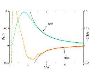
Figure 5: Interface potential (squares) and disjoining pressure (circles) of a model of Argon adsorbed on solid Carbon Dioxide. The dashed lines are a guide to the eye, while the full monotonic lines depict the power law decay expected from the step density model with van der Waals forces (results adapted from Ref.[45, 53], correspond to the same model and temperature as the three preceding figures).

Obviously, a more accurate expression is obtained if we use Eq. (35) for the film profile. Unfortunately, the resulting integral does not have a primitive that will provide us with much insight. It is more convenient to consider a superposition approximation, but still using the step–like model for the liquid–vapor interface, such that:

$$\rho(z;\ell)=[1+h_{\rm wl}(z)][\rho_{l}-\Delta\rho_{\rm lv}\mathcal{H}(z-\ell)]$$ (40)

Rather than trying to solve for $g_{V}(\ell)$, which is also quite unpleasant, we consider the disjoining pressure, which may be obtained from $g_{V}$ as:

$$\Pi_{V}(\ell)=-\frac{dg_{V}(\ell)}{d\ell}=-\int_{d_{\omega}}^{\infty}V(z)\frac{d\rho(z;\ell)}{d\ell}$$ (41)

whence, by virtue of the second equality, the Heaviside step function is transformed into a Dirac function and projects the integrand out, yielding:

$$\Pi_{V}(\ell)=[1+h_{\rm wl}(\ell)]\frac{H_{w}}{6\pi}\ell^{-3}$$ (42)

It follows that, apart from the well known leading order contribution to the disjoining pressure of long–range fluids, our mean field calculations provide an additional oscillatory contribution with a fast decay of order $e^{-b_{o}\ell}/\ell^{3}$. It is also worth noticing that, as successive derivatives of the interface potential are performed, the decay of van der Waals tails becomes steeper, whereas that of short range forces (c.f. Eq. (36)) remains of the same range. Accordingly, it could be possible to find a crossover from long–range to short–range dominated interactions in either $\Pi(\ell)$ or its derivatives. This has been considered as a possible hypothesis for the explanation of experimental findings that we will discuss later [86, 87].

Figure 5 shows computer simulation results for the interface potential of Argon adsorbed on a solid substrate close to the wetting temperature [53]. The interface potential presents a minimum corresponding to metastable equilibrium thin films, and a long–range monotonic decay which, as shown in the figure, may be nicely described from the expected power law of Eq. (39). The disjoining pressure may be calculated from $g(\ell)$ by derivation and is also shown in Fig.5. Upon numerical derivation, the highly accurate data for $g(\ell)$ reveals oscillatory behavior completely washed out in the interface potential. Such oscillatory behavior is the result of the layered structure of the adsorbed films (c.f. Fig.4). The figure shows that the oscillations are superimposed on the expected leading order monotonic decay of $\ell^{-3}$, as suggested from Eq. (42).

The almost quantitative description of the density profiles afforded by Eq. (35), and the qualitative description of the interface potential and disjoining pressure afforded by Eq. (39) and Eq. (42), are a pleasing accomplishment of liquid state theory. If, however, we attempted to describe the oscillations exhibited by the disjoining pressure from the known correlation function $h_{\rm wl}$, as suggested by Eq. (42) we would find predicted oscillations with amplitudes that are far too large.

Why are the results of simulation so much smoothed relative to the theoretical expectations of liquid state theory will be discussed in the next section.

3 Classical Capillary Wave Theory

In the previous section we have seen that Density Functional Theory provides a consistent and unified framework for the description of a purely flat interface, where the density profile is only a function of the perpendicular direction, $z$. Not unexpectedly, we have found that the structural properties of the interface, as well as the interface potential and disjoining pressure are intrinsic properties of the fluid, i.e.: they only depend on the fluid’s structural properties and on the intensive thermodynamic fields (temperature and chemical potential).

In practice, however, one can hardly expect the dividing surface of a film to remain flat at finite temperature. Rather, it is expected that thermal fluctuations will deform the interface, such that it becomes rough and accordingly the film profile deviates from its average value. Such capillary waves may be described in terms of the Monge representation, where the film thickness above a point $\mathbf{x}$ on a reference plane is given as a smooth function $\ell(\mathbf{x})$ (c.f. Fig.6). Obviously, this description ignores overhangs and bubbles but should be quite reliable away from the bulk critical point. Fluctuations of $\ell(\mathbf{x})$ away from the average increase the entropy of the interface, but are at the cost of increasing the surface area. Furthermore, whether the film is adsorbed on a substrate, or subject to the effect of gravity, it will feel an external field that restricts the fluctuations of $\ell(\mathbf{x})$ via the interface potential $g(\ell)$. This physical situation clearly calls for a description in terms of the Interfacial Hamiltonian described in the introduction, Eq. (1). In this context, we will also refer to IHM, as the capillary wave Hamiltonian, CWH.

In order to avoid confusion between the rough interface profile, $\ell(\mathbf{x})$, and its thermal average, denoted $\ell$ in the previous section, we will usually refer to $\ell(\mathbf{x})$ as $\Sigma$ (for sinusoidal interface). In some instances, we will also use the label $\pi$ (short for planar) in order to stress the difference between properties of a rough interface and those of an assumed planar interface.

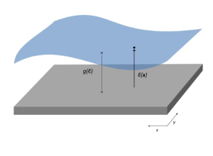
Figure 6: Sketch of the rough interface of an adsorbed film subject to an external field. For each point $\mathbf{x}$ on the plane of the substrate, a film height $\ell(\mathbf{x})$ is defined, and a local free energy calculated as $g(\ell(\mathbf{x}))d\mathbf{x}$.

3.1 Capillary wave spectrum

Let us now consider to what extent do thermal capillary waves modify the structure of the interface as described in the previous section. As we will show, the consequences are actually very important, already at the lowest order of approximation.

First, we consider the limit of small gradients, $(\nabla\ell)^{2}\ll 1$. This allows us to get rid of the unpleasant square root, and write:

$$H[\Sigma]=\int d\mathbf{x}\left\{g(\ell(\mathbf{x}))+\frac{1}{2}\gamma_{\infty}[\nabla\ell(\mathbf{x})]^{2}\right\}$$ (43)

where, as explained above, $\Sigma$ is a shorthand for the functional dependence of $\ell(\mathbf{x})$. Despite the apparently very different physics, the capillary wave Hamiltonian is formally identical to the square gradient functional (c.f. Eq. (16)), with $\ell(\mathbf{x})$ playing the role of $\rho(\mathbf{r})$ and $\gamma_{\infty}$ the role of $C_{\infty}$. Relating $\rho(\mathbf{r})$ with $\ell(\mathbf{x})$ allows us to transform the gradient of densities into a gradient of $\ell(\mathbf{x})$ and identify the Square Gradient Functional with $H[\Sigma]$ [37, 34] to leading order, as we shall see in section 5.

In order to proceed, we expand the integrand in small deviations away from the average film height. Defining $\delta\ell(\mathbf{x})=\ell(\mathbf{x})-\ell$, and performing a Taylor series of $g(\ell)$ leads to:

$$H[\Sigma]=\int d\mathbf{x}\left(g(\ell)+g^{\prime}(\ell)\delta\ell+\frac{1}{2}g^{\prime\prime}(\ell)\delta\ell^{2}+\frac{1}{2}\gamma_{\infty}(\nabla\ell(\mathbf{x}))^{2}\right)$$ (44)

It is now convenient to describe the film height fluctuations in terms of Fourier modes, $\delta\ell_{\mathbf{q}}$, as follows:

$$\delta\ell(\mathbf{x})=\sum_{\mathbf{q}}\delta\ell_{\mathbf{q}}e^{i\mathbf{q}\cdot\mathbf{x}}$$ (45)

Plugging this result back into equation Eq. (44), followed by some rearrangements, then yields:

$$\begin{array}[]{lll}H[\Sigma]&=&Ag(\ell)+\int d\mathbf{x}\left[g^{\prime}(\ell)\sum_{\mathbf{q}}\delta\ell_{\mathbf{q}}\,e^{i\mathbf{q}\cdot\mathbf{x}}+\right.\\ &&\\ &&\left.\frac{1}{2}\sum_{\mathbf{q}}\sum_{\mathbf{q}^{\prime}}\left(g^{\prime\prime}(\ell)+\gamma_{\infty}\,\mathbf{q}\cdot\mathbf{q}^{\prime}\right)\delta\ell_{\mathbf{q}}\delta\ell_{\mathbf{q}^{\prime}}\,e^{i(\mathbf{q}+\mathbf{q}^{\prime})\cdot\mathbf{x}}\right]\end{array}$$ (46)

where $A$ is the surface area of the flat interface. The integral over $\exp(i\mathbf{q}\cdot\mathbf{x})$ is $A\,\delta_{\mathbf{q},0}$, while that over $\exp{\left[i(\mathbf{q}+\mathbf{q}^{\prime})\cdot\mathbf{x}\right]}$ is likewise $A\,\delta_{\mathbf{q},-\mathbf{q}^{\prime}}$, with $\delta_{\mathbf{q},\mathbf{q}^{\prime}}$, Kronecker’s delta [88]. Furthermore, we take into account that by definition, $\delta\ell(\mathbf{x})$ describes fluctuations about the average film height, so that the zero wave vector mode $\delta\ell_{\mathbf{q}=0}$ is null. With this in mind, we can now integrate Eq. (46), to obtain:

$$H[\Sigma]=A\left\{g(\ell)+\frac{1}{2}\sum_{\mathbf{q}}[g^{\prime\prime}(\ell)+\gamma_{\infty}q^{2}]|\delta\ell_{\mathbf{q}}|^{2}\right\}$$ (47)

This result provides us with the free energy of a frozen realization of the interfacial roughness. We can define the probability of such realization with the usual Boltzmann weight:

$$P(\Sigma)=\frac{e^{-\beta H(\Sigma)}}{Z_{cw}}$$ (48)

where $Z_{cw}$, the partition function, is now a sum over all possible capillary wave realizations. In terms of the capillary wave modes, this can be written as:

$$Z_{cw}=\int\prod d\ell_{\mathbf{q}}\,e^{-\beta H[\Sigma]}$$ (49)

Since $H$ is given in terms of independent additive Fourier mode contributions, it can be factored into a product of simple integrals as in the case of the partition function of an ideal gas, so that we can write:

$$Z_{cw}=e^{-\beta Ag(\ell)}\prod_{\mathbf{q}}\int d\ell_{\mathbf{q}}e^{-\frac{1}{2}\beta A[g^{\prime\prime}(\ell)+\gamma_{\infty}q^{2}]|\delta\ell_{\mathbf{q}}|^{2}}$$ (50)

Taking into account that $|\delta\ell_{\mathbf{q}}|^{2}$ is actually the complex squared modulus of $\delta\ell_{\mathbf{q}}$, it follows that the integral is of Gaussian form. Despite some subtleties related to integration in the complex plane [89, 88], it satisfies the equipartition theorem. Considering $|\delta\ell_{\mathbf{q}}|^{2}$ to play the role of squared velocity and $A[g^{\prime\prime}(\ell)+\gamma_{\infty}q^{2}]$ the role of mass, we can then write:

$$A\langle\delta\ell_{\mathbf{q}}\delta\ell_{-\mathbf{q}}\rangle=\frac{k_{B}T}{g^{\prime\prime}(\ell)+\gamma_{\infty}q^{2}}$$ (51)

where the angle brackets denote a thermal average.

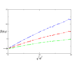
Figure 7: Plot of the effective wave–vector dependent surface tension (left hand side of Eq. (52)). Results are displayed for the liquid–vapor interface of a Lennard–Jones model of Argon close to the triple point (the model and temperature are as studied in Ref.[45], employed in Fig.2–5 and described in more detail in sec.4.3). The symbols are simulation data obtained for three different choices of the interface position, and the lines are a guide to the eye. The arrow indicates independent results for the liquid–vapor surface tension [53].

This result states that the mean squared amplitude of the Fourier modes decreases as the square of the in–plane wave vector increases. Such expectation has been confirmed in a great number of computer simulation studies for the special cases of free–interfaces, i.e., in the absence of external fields, whence $g^{\prime\prime}(\ell)=0$. In this simple case, one can arrange Eq. (51) as:

$$\frac{1}{Aq^{2}\langle|\delta\ell_{\mathbf{q}}|^{2}\rangle}=\beta\gamma_{\infty}$$ (52)

It follows that a plot of the left hand side as a function of $q^{2}$ is a constant equal to the surface tension. In practice, for the small systems that are usually considered in computer simulation studies, it is difficult to achieve the regime where Eq. (52) is actually constant, but the results may be safely extrapolated to $q=0$ and provide good estimates of the surface tension [90, 91, 92, 93] or even the stiffness of solid–fluid interfaces above the roughening transition [94, 95, 96].

For the large $q$ regime that is achievable in simulations, it is found that the left hand side of Eq. (52) provides a phenomenological definition for a wave vector dependent surface tension $\gamma(q)$, describing the deviations of $\langle|\delta\ell_{\mathbf{q}}|^{2}\rangle^{-1}$ from the expected low $q$ regime of $\beta\gamma_{\infty}$ [85, 49]. From theoretical considerations, it is known that the linear term in $\gamma(q)$ is absent, so that, to lowest order, one can write [85, 97]:

$$\gamma(q)=\gamma_{\infty}+\kappa q^{2}$$ (53)

where $\kappa$ is known as the bending rigidity.

Figure 7 shows a plot of the left hand side of Eq. (52), as a function of $q^{2}$, as obtained for a liquid–vapor interface of a Lennard–Jones model of Argon. Since the definition of the interface down to atomic length scales has some degree of arbitrariness (this will be discussed at length in section 4.1), the spectrum depends on the actual criteria that are employed to locate it. Results for three different choices of the interface position are presented in the figure. Whereas all such choices yield different results, it is clear that 1) all the spectra extrapolate to the same $q=0$ value, coincident with the liquid–vapor surface tension obtained independently and indicated in the figure with an arrow and 2), in a regime of long wave–vectors up to about $q=2$ inverse molecular diameters, a clearly linear behavior is found consistent with Eq. (53).

Two important considerations are worth mentioning at this stage:

1) Exactly how the square gradient coefficient of the CWH, $\gamma_{\infty}$ is related to the actual liquid–vapor surface tension has been the matter of debate for a long time (see an interesting review by Gelfand and Fisher for further details on this issue [98]). In the original formulation of Buff, Stillinger and Lovett [28], $\gamma_{\infty}$ was considered an effective free energy, smaller than the experimental tension by terms of order $q_{\rm max}^{2}$, with $q_{\rm max}$ an upper cutoff wave–vector. However, ample theoretical and simulation evidence has gathered favoring the interpretation of $\gamma_{\infty}$ as the actual experimentally accessible liquid–vapor surface tension [99, 100, 92, 101], or at least, as a finite system size approximation [89, 102, 98]. The explicit form of the finite size dependence is also a matter of debate, but simulation results suggest that the dependence is weak [103, 104, 105]. For this reason, in what follows we will refer to $\gamma_{\infty}$ as the macroscopic liquid–vapor surface tension. Rather, anticipating results of section 5, we employ the subindex $\infty$, in order to stress we refer here to the surface tension in the absence of an external field, i.e. at infinite distance away from the field.

2) Intuitively, a positive slope of the phenomenological $\gamma(q)$ is in principle expected, since, a negative slope would imply apparently unphysical diverging low wavelength interfacial fluctuations. However, it has been suggested that fluids with van der Waals interactions have a negative effective bending rigidity, with $\gamma(q)$ exhibiting a minimum at finite $q$ and then increasing as expected for large $q$ [85]. This hypothesis, which has been supported by experiments [49], is however still to date subject to some reservations [106, 107, 108]. Clearly, the results of Fig.7 illustrate the difficulties of defining unambiguously a bending rigidity, since it depends on the somewhat arbitrary procedure employed for the precise location of the interface [106, 109].

3.2 The interfacial roughness

Unfortunately, except for very few instances [49] and some reservations [107], grazing x–ray scattering studies do not provide the resolution that is required to test the full capillary wave spectrum, i.e., Eq. (51) (c.f. Ref.[108] and [110] for reviews on x–ray scattering studies of surfaces). Rather, it is the interfacial roughness $\Delta_{\rm cw}^{2}=\langle\delta\ell^{2}\rangle$ that is usually measured, whether one considers the free fluid interface [111, 112, 113], or that of adsorbed films [114, 48, 115, 116].

Using Plancherel’s theorem, it is possible to relate the lateral average of $\delta\ell^{2}$ with that of $\delta\ell_{\mathbf{q}}\cdot\delta\ell_{-\mathbf{q}}$, so that the roughness may be determined by summation of the thermally averaged squared Fourier modes as:

$$\Delta_{\rm cw}^{2}=\sum_{\mathbf{q}}\langle\delta\ell_{\mathbf{q}}\cdot\delta\ell_{-\mathbf{q}}\rangle$$ (54)

Considering the transformation $\sum_{\mathbf{q}}\rightarrow\frac{A}{4\pi^{2}}\int\int dq_{x}dq_{y}$ we can evaluate the interfacial roughness as the integral of Eq. (51):

$$\Delta_{\rm cw}^{2}=\frac{k_{B}T}{2\pi}\int_{q_{\rm min}}^{q_{\rm max}}\frac{q\,dq}{g^{\prime\prime}(\ell)+\gamma_{\infty}q^{2}}$$ (55)

where, by virtue of the isotropy of the interface in the transverse direction, we have transformed $dq_{x}dq_{y}$ into $2\pi qdq$. The lower bound of the integral $q_{\rm min}=2\pi/L$ is given by the finite system size of the simulation, or by the experimental setup. Unfortunately, the integral does not converge, and an ad hoc maximum wave–vector cutoff $q_{\rm max}$ has to be introduced. This is not always a problem in experimental studies, since the maximal wave–vector can be identified with an instrumental cutoff related to the maximal momentum transfer, but does become an unpleasant problem in simulation studies, where the resolution goes down to the atomic scale. In practice, one assumes $q_{\rm max}=2\pi/\lambda_{\rm min}$, with $\lambda_{\rm min}$ an empirical parameter which has been interpreted either as an atomic length scale [113], or the bulk correlation length [89, 117]. The difference is of little consequence at low temperature, but should be a matter of concern as the critical point is approached.

Performing the integral, Eq. (55), we obtain finally the capillary–wave–induced interfacial roughness:

$$\Delta^{2}_{cw}=\frac{k_{B}T}{4\pi\gamma_{\infty}}\ln\frac{1+\xi_{\parallel}^{2}q_{\rm max}^{2}}{1+\xi_{\parallel}^{2}q_{\rm min}^{2}}$$ (56)

where the relevant length scale here:

$$\xi_{\parallel}=\sqrt{\frac{\gamma_{\infty}}{g^{\prime\prime}}}$$ (57)

is known as the parallel correlation length and dictates the range of capillary wave fluctuations in the transverse direction [55, 54]. For liquid–vapor interfaces under gravity, $\xi_{\parallel}$ may be immediately identified with the capillary length, $a$. For films adsorbed on a substrate, it is also sometimes known as the healing distance [30], and dictates the ability of a liquid film to match the roughness of the underlying substrate [21, 47, 30]. On the other hand, $\Delta_{\rm cw}^{2}$ is also some times known as the perpendicular correlation length, and written alternatively as $\xi_{\perp}$. Table 1 provides a list of parallel and perpendicular correlation lengths for different important intermolecular forces acting on the liquid–vapor interface.

		External Field
		System Size	Short Range	van der Waals	Gravity
$g(\ell)$		-	$D\exp(-b\ell)$	$\frac{H_{w}}{12\pi}\ell^{-2}$	$\frac{1}{2}m\Delta\rho G\ell^{2}$
$\xi_{\parallel}^{2}$		$\gg L^{2}$	$\frac{\gamma_{\infty}}{Db^{2}}\exp(b\ell)$	$\frac{2\pi\gamma_{\infty}}{H_{w}}\ell^{4}$	$\frac{\gamma_{\infty}}{m\Delta\rho G}$
$\Delta_{\rm cw}^{2}$		$\ln L$	$\ell$	$\ln\ell$	$\ln a$

Table 1: Table of interface potentials, $g(\ell)$ and parallel correlation lengths, $\xi_{\parallel}$ for common external fields acting on an interface. The last row indicates the leading order dependence of the capillary roughness, $\Delta_{\rm cw}^{2}$ that results. $D$ is the amplitude of short range forces, and has dimensions of energy per unit area. When $1/b$ is identified with the Debye screening length, the results may describe interactions arising from the electric double layer.$H_{w}$ is the Hamaker constant. $a^{2}=\gamma_{\infty}/m\Delta\rho G$, with $G$ the acceleration of gravity, is the squared capillary length.

The above result is of experimental relevance in two limiting cases.

Weak fields

For very weak external fields, the parallel correlation length becomes very large, and may actually achieve values much larger than the lateral system size. In this case, $\xi_{\rm\parallel}\,q_{\rm min}\gg 1$ and the capillary wave roughness becomes:

$$\Delta^{2}_{cw}=\frac{k_{B}T}{2\pi\gamma_{\infty}}\ln\frac{q_{\rm max}}{q_{\rm min}}$$ (58)

This result implies a logarithmic dependence on system size $L$ (simulations) or experimental lower cutoff $\lambda_{\rm min}$ which has been fully confirmed. The most natural way to study this limit is a computer simulation study, where one can prepare a liquid slab inside a simulation cell at zero field. In practice, however, the capillary length for essentially all liquids is so much larger than the upper wavelength cutoff afforded with scattering techniques that also ordinary fluid interfaces under the effect of gravity are in this limit. Indeed, both computer simulations [118, 119, 101, 120] and experimental studies [111, 121, 48] agree as to the logarithmic dependence of the interfacial roughness, and confirm that the slope of $\Delta^{2}_{cw}$ as a function of $\ln q_{\rm min}$ yields a reliable estimate of the surface tension [118, 119, 101, 122, 123, 120, 96].

Strong fields

If, on the other hand, the interface is subject to a strong field, as is the case for a thin adsorbed film subject to a disjoining pressure, the parallel correlation length is small but $\xi_{\rm\parallel}q_{\rm max}$ usually remains much larger than unity. In most practical realizations, however $\xi_{\rm\parallel}q_{\rm min}\ll 1$ and, as a result the roughness is no longer system size dependent:

$$\Delta^{2}_{cw}=\frac{k_{B}T}{2\pi\gamma_{\infty}}\ln(\xi_{\parallel}q_{\rm max})$$ (59)

In this equation, $\xi_{\parallel}$ plays a similar role as $q_{\rm min}^{-1}$ in the weak field limit. Also in this case, there is a large amount of evidence strongly in favor of a logarithmic dependence of $\Delta^{2}_{cw}$ on $\xi_{\parallel}$. In most practical realization, the adsorbed liquid film is subject to van der Waals forces, so that the liquid–vapor interface is bound by an interface potential $g(\ell)\propto\ell^{-2}$. As a result, the interfacial roughness exhibits a logarithmic dependence on the film thickness (c.f. Table 1), and a fit to the experimental data actually provides reasonable estimates of the Hamaker constant [47, 48, 124, 115, 116]. An even more striking confirmation of this result is afforded in systems where the Hamaker constant is very small. In such cases, the dominant contribution stems from short range forces. The interface potential is now of the form, $g(\ell)\propto e^{-\ell}$, so that the capillary wave roughness grows as the square root of the film thickness increases, as illustrated in Table 1 [125, 126, 123].

Despite this amount of experimental evidence, the situation of Eq. (56) seems far less satisfactory in the strong field limit than it is for the weak field limit. Indeed, many studies report a capillary roughness that is either too large [116] or too small [115] relative to expectations from Eq. (59), while other studies find the logarithmic prefactor incompatible with the known interfacial tension [115, 48]. In some instances, these discrepancies have been attributed to a possible cross–over from long–range ($\xi_{\parallel}\propto\ell^{-4}$) to short–range forces ($\xi_{\parallel}\propto\exp(-\ell)$) [86, 87]; while in others it has been suggested the need to somehow incorporate a film–thick–dependent interfacial tension [86, 115]. Be as it may, the long wavelength dependence of Eq. (56) is essentially uncontested and remains to date the framework for experimental analysis.

As a final comment, it is worth mentioning that considering explicitly the wave–vector dependent surface tension as dictated by Eq. (53) into the capillary spectrum of Eq. (51), would in principle allow to eliminate the need for an empirical upper wave–vector cutoff. Indeed, the Fourier amplitudes are then given by:

$$A\langle\delta\ell_{\mathbf{q}}\delta\ell_{-\mathbf{q}}\rangle=\frac{k_{B}T}{g^{\prime\prime}(\ell)+\gamma_{\infty}q^{2}+\kappa q^{4}}$$ (60)

For positive $\kappa$ at least, the integral now converges and needs not the upper cutoff [110, 97, 108]. Unfortunately, the resulting expression, which is far less convenient, has been seldom employed [110, 127, 128].

3.3 Intrinsic and capillary wave broadened profiles

The prediction of large perpendicular interfacial fluctuations $\Delta^{2}_{\rm cw}$ for a liquid–vapor interface poses a serious challenge to the traditional view of a well defined, intrinsic density profile, say, $\rho_{\pi}(z)$, as described in section 2. According to the picture that emerges from Eq. (56), the liquid–vapor interface of a substance on earth exhibits almost unbound perpendicular fluctuations up to the capillary length, which, for a fluid such as water at ambient temperature is on the $mm$ length scale. This implies that a fixed point $z$ say a $\mu m$ away from the equimolar dividing surface, is found alternatively within the liquid or vapor phases, such that its average density is simply half way between $\rho_{l}$ and $\rho_{v}$. A pessimistic interpretation of this result is that, in the absence of the gravitational field the liquid-vapor interface cannot possibly exist in the thermodynamic limit. This view relies too heavily on the significance of averages, particularly those collected over an infinite period of time (an analogous interpretation would imply that Brownian particles do not move, because their average position is zero, whereas we know that the most likely event is that each such particle in a sample would have moved away from the original position as $\sqrt{t}$). In practice, the relaxation dynamics of the capillary waves is also very slow [129] and there is no problem in identifying the interface over long but finite periods. Furthermore, it has been shown that the intrinsic density profile is always recognizable at the scale of the bulk correlation length, provided it is measured relative to the instantaneous interface position [99].

For small systems, however, even a small observation time as is usually afforded in computer simulations or x-ray scattering experiments produces an averaged density profile which exhibits the fingerprints of capillary wave broadening. The connection between the average density profile that can be actually measured and the underlying intrinsic density profile relevant to length–scales below the bulk correlation length may be performed by means of a convolution [99, 130, 102, 131], as we shall soon see. First, however, consider the picture that emerges from the capillary wave theory: a local displacement of the interface about its average, $\delta\ell(\mathbf{x})$, translates the whole density profile by exactly that amount, such that the instantaneous density becomes $\rho_{\pi}(z-\delta\ell)$. To see how this changes the measured average density, let us Taylor expand the translated profile about $z$:

$$\rho(\mathbf{r};\Sigma)=\rho_{\pi}(z)-\rho^{\prime}_{\pi}(z)\delta\ell(\mathbf{x})+\frac{1}{2}\rho^{\prime\prime}_{\pi}(z)\delta\ell(\mathbf{x})^{2}$$ (61)

Performing now a lateral average, the linear term in $\delta\ell(\mathbf{x})$ vanishes, but the quadratic term does not. It is then apparent that, for a fluctuating interface, the averaged density $\rho(z;\Sigma)$ cannot possibly be equal to the intrinsic density profile, but rather is:

$$\rho(z;\Sigma)=\rho_{\pi}(z)+\frac{1}{2}\rho^{\prime\prime}_{\pi}(z)\langle\delta\ell(\mathbf{x})^{2}\rangle$$ (62)

Since, for reasons of symmetry, the probability of exhibiting translations to the left or to the right must be equal for a free interface, we expect a Gaussian distribution for $\ell(\mathbf{x})$, with width equal to $\langle\ell(\mathbf{x})^{2}\rangle$. Whence, alternatively to the series representation of Eq. (62), we can write the effect of the interface translations by means of a convolution, as follows [99, 130, 102, 131]:

$$\rho(z)=\int\rho_{\pi}(z-\ell)P(\ell)d\ell$$ (63)

where $P(\ell)$ is the probability density for the interface displacements. The theoretical expectation of a Gaussian distribution of width $\Delta_{\rm cw}$ has been convincingly confirmed in numerous computer simulation studies [131, 123, 101], so that we can safely assume [99, 130]:

$$P(\delta\ell)=\frac{1}{\sqrt{2\pi\Delta_{\rm cw}^{2}}}e^{-\frac{1}{2}\frac{\delta\ell^{2}}{\Delta_{\rm cw}^{2}}}$$ (64)

Fig.8 displays the probability distribution of the local interface position for the liquid–vapor interface of a Lennard–Jones like Argon model at moderate temperature. The results are given for systems with increasing lateral system size and clearly show that the probability distribution is Gaussian, becoming flatter as the lateral area increases.

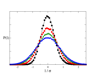
Figure 8: Probability distribution of local film thickness of a liquid–vapor interface at moderate temperature as described by the Lennard–Jones model of Argon. Results are depicted for system sizes with lateral area of $100$ (black), $200$ (red), $300$ (green) and $400$ (blue) squared molecular diameters, $\sigma$. Symbols are results from simulation, while the lines are Gaussian fits (results from Ref.[132] at $k_{B}T=0.90\epsilon$, c.f. Sec. 4.3 for more details on the model).

The role of capillary roughening is perhaps best illustrated using the most crude possible description for the intrinsic profile, i.e., a simple step function of the form:

$$\rho_{\pi}(z)=\frac{1}{2}(\rho_{l}+\rho_{v})-\frac{1}{2}(\rho_{l}-\rho_{v})(2\mathcal{H}(z)-1)$$ (65)

with $\mathcal{H}(z)$ the Heaviside function. The convolution of Eq. (64) transforms the discontinuous step–like density profile into a smooth error function of width $\sqrt{2}\,\Delta_{\rm cw}$ [130]:

$$\rho(z)=\frac{1}{2}(\rho_{l}+\rho_{v})-\frac{1}{2}(\rho_{l}-\rho_{v}){\rm Erf}(\frac{z}{\sqrt{2}\,\Delta_{\rm cw}})$$ (66)

It is a remarkable achievement of mathematical physics to show that, for the free interface of a two dimensional Ising model, Eq. (66), with $\Delta_{\rm cw}$ given by Eq. (58), follows exactly from the underlying microscopic Hamiltonian [100, 133].

According to the above equation, in the weak field limit, where $\Delta^{2}_{\rm cw}\propto\ln L$, the averaged profile becomes completely smoothed out for $L\to\infty$. For finite system sizes, the effect is also apparent and measurable. Figure 9 displays density profiles for adsorbed films of the Lennard–Jones Argon model above the wetting transition for several system sizes. The film is stratified as is usual for atomic fluids (inset), but a closer look clearly shows how the liquid–vapor interface decays over larger and larger length scales as the lateral system size is increased. The broadening of the density profile may be measured and tested against expectations from Eq. (56), providing an independent means of estimating the surface tension [118, 119, 101, 122, 134, 123, 120, 96].

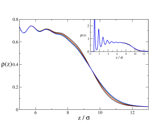
Figure 9: Detailed view of the liquid–vapor density profile of an adsorbed Lennard–Jones fluid above the wetting transition. Results are given for systems with lateral area increasing from 100 to 400 squared molecular diameters, $\sigma$, in the order black, red, green, blue. The inset displays the overall view of the density profile, where it becomes clear that the broadening only affects the liquid–vapor interface, but not the layered structure (results from [132], the model is as that employed in [45] and described in Sec. 4.3, with an increased wall strength of $\epsilon_{w}=143\epsilon\sigma^{3}$ and a temperature of $k_{B}T=0.90\epsilon$).

Actually, the result of Eq. (66) serves as starting point for the analysis of most experimental studies on capillary waves [108, 111, 112, 114, 113, 124, 48, 110, 115, 116, 121, 127, 87]. Low grazing beams on a surface produce scattering intensities which probe the density profile along a direction perpendicular to the interface. For the simple case of a single moderately rough interface, the reflectivity is given by [108, 114, 115]:

$$R(Q)\propto\left|\int dz\frac{d\langle\rho\rangle}{dz}e^{iQz}\right|^{2}$$ (67)

where $Q$ is a scattering vector. Using Eq. (66) into the scattering formula, it is found that the capillary waves result in a Debye–Waller like attenuation factor for the reflectivity: [108, 113, 124, 122]:

$$R(Q)\propto e^{-Q^{2}\Delta_{\rm cw}^{2}}$$ (68)

Accordingly, a plot of $\ln R(Q)$ against $Q^{2}$ provides a straight line with a slope equal to the capillary roughness. In practice, however, the intrinsic density profile is not an infinitely steep step function, but has its own intrinsic width. As a result, the interfacial width that is measured in scattering experiments has both intrinsic and capillary wave contributions, and one usually assumes that the actual measured roughness, say, $\Delta_{\rm exp}$ is given by [113, 124, 115, 116, 127]:

$$\Delta_{\rm exp}^{2}=\Delta_{\pi}^{2}+\Delta_{\rm cw}^{2}$$ (69)

where $\Delta_{\pi}^{2}$ is attributed to the intrinsic density profile. This is not an all together convenient situation, since $\Delta_{\pi}^{2}$ cannot be measured independently, so that it adds to the upper cutoff $q_{\rm max}$ yet another empirical parameter. Unfortunately, one cannot actually resolve $\Delta_{\pi}$ from the $\ln q_{\rm max}$ contribution of $\Delta_{\rm cw}$, and there are no other ways to distinguish from one another than plausible arguments. In principle, the situation could be remedied by assuming a reasonable intrinsic density profile, and performing the convolution of Eq. (63). In practice, however, the convolution cannot be obtained analytically, not even for the simple $\tanh(z)$ function, and only occasionally it is performed numerically [123, 92, 121, 122]. For that reason, either ${\rm Erf}$ or $\tanh$ functions are employed to fit the density broadened profiles, and $\Delta_{\rm cw}$ is obtained as a fitting parameter. There is however some evidence that the ${\rm Erf}$ profile is a better choice [119].

Surprisingly, the fact that the double–parabola model provides an analytic expression for the convolution has not been recognized. Indeed, plugging Eq. (22) into Eq. (63), and using Eq. (64), yields, for the broadened density profile the following lengthy but convenient result:

$$\rho(z)=\rho_{\rm step}(z)+\Delta\rho_{\rm str}(z)$$ (70)

where $\rho_{\rm step}(z)$ is the leading order broadening from the structure–less step model (Eq. (66)), and $\Delta\rho_{\rm str}(z)$ is the additional contribution due to the intrinsic interfacial structure [64]:

$$\begin{array}[]{lll}\Delta\rho_{\rm str}(z)&=&\frac{1}{2}\frac{\rho_{l}-\rho_{v}}{b_{l}+b_{v}}\left\{b_{l}e^{-b_{v}(z-\frac{1}{2}b_{v}\Delta_{\rm cw}^{2})}{\rm Erfc}\left(-\frac{z-b_{v}\Delta^{2}_{\rm cw}}{\sqrt{2}\Delta_{\rm cw}}\right)\right.\\ &&\\ &&-\left.b_{v}e^{b_{l}(z+\frac{1}{2}b_{l}\Delta_{\rm cw}^{2})}{\rm Erfc}\left(\frac{z+b_{l}\Delta^{2}_{\rm cw}}{\sqrt{2}\Delta_{\rm cw}}\right)\right\}\end{array}$$ (71)

Using this equation to fit the reflectivity data would allow to resolve the capillary wave roughness $\Delta_{\rm cw}$ from the intrinsic structure, as well as to obtain an estimate of the bulk correlation lengths. One could then extract $q_{\rm max}$ meaningfully from $\Delta_{\rm cw}$, and compare $\lambda_{\rm min}=2\pi/q_{\rm max}$ with the bulk correlation lengths obtained from the fit.

To sum–up, we have shown that thermal capillary waves considerably modify the structure of the interface, conveying information on the whole system size into the otherwise intrinsic density profile. We have shown that the predictions of the classical capillary wave theory seem very well tested for interfaces subject to a weak field, but some discrepancies seem to arise for adsorbed films subject to relatively strong fields. Unfortunately, comparisons between theory and experiment are not straightforward, because experimentally only the capillary roughness is usually accessible. A much more stringent test could be achieved if the whole capillary wave spectrum of adsorbed films were measured. Since x–ray measurements are still very difficult to achieve at the level of resolution that is sought, computer simulations would seem an ideal tool. In the next section we will review current state of the art methods for the computer simulation of the spectrum of adsorbed films.

4 Computer simulations of the capillary wave spectrum of adsorbed films

Computer simulations are an invaluable tool for the study of adsorption phenomena [15]. Certainly, they have provided great insight and a complementary perspective for the interpretation of different very relevant experimental and theoretical findings. As a notable example, we can mention studies on wetting and prewetting transitions [135, 136, 137, 138] which parallel the first few experimental reports [139, 140] performed some years after the theoretical predictions [69]. Countless other examples could be mentioned, but we will narrow this broad area and focus merely on the study of capillary wave fluctuations of adsorbed films.

It is surprising to see that, despite the great number of studies on capillary waves of free interfaces, only a few have been performed for the case of adsorbed films. Similar to experimental realizations, most of such studies have focused on the analysis of capillary wave broadening. The findings reported clearly indicate an interfacial roughness qualitatively in agreement with $Eq.~{}(\ref{eq:ccwrsf})$, both as regards the expected decrease with increasing field strength and the predicted increase with system size. However, a full quantitative agreement has not been obtained, even though one has at hand both the upper wave–vector cutoff, $q_{\rm max}$, and the intrinsic interfacial roughness $\Delta_{\pi}$ as fitting parameters. Of particular interest is reference [86], where a liquid–liquid interface of inmiscible polymer phases subject to van der Waals forces was studied. In this paper, it was indicated that the simulation results could be only described if either, i) a film thick dependent interfacial width $\Delta_{\pi}$, or ii) a film-thick dependent surface tension was incorporated into the classical theory. Interestingly, these observations are in agreement with experimental findings on a related system [115].

These studies notwithstanding, a detailed analysis of the full capillary wave spectrum of adsorbed films has not been performed until very recently [50, 51, 45]. This provides a very stringent test of the classical theory, but requires dealing with two important difficulties before the problem can be successfully tackled. Firstly, one needs to carefully implement a practical methodology for defining the film profile that is sufficiently robust to work also as the film thins. Secondly, it is required to have adequate simulation techniques to asses independently the main properties that are provided by the capillary wave spectrum, namely, the interface potential and the surface tension. Let us now address each of these issues briefly.

4.1 Characterization of film profiles

Despite that the concept of “surface” is intuitive and familiar, the mathematical problem of defining an interface from atomic scale data is surprisingly difficult and subject to arbitrariness. The problem is that our intuition relies on the description of surfaces at large wavelengths, where the continuity of such objects is not an issue. In molecular simulations, however, one deals with sets of atomic positions, so that the data available is essentially discrete. Thus, the only possible way out is to define a set of criteria which will allow us to determine a smooth function $\ell(\mathbf{x})$ from the discrete atomic positions [131, 123, 141, 94, 142, 95, 120].

The selected criteria should provide a mathematical surface, $\ell(\mathbf{x})$, that allows, on the one hand, to calculate a capillary wave spectrum for comparison with Eq. (51), and on the other hand, to resolve the intrinsic density profile $\rho_{\pi}(z)$ from the capillary wave fluctuations.

An apparently very simple procedure rooted on surface thermodynamics is to divide the system into a set of $n$ elongated prisms of square basis and fixed lateral area $A/n$ [123, 86, 92]. For prism $i$ one calculates the lateral average density $\rho_{i}(z)$ and defines the interfacial height $\ell_{i}$ as the corresponding equimolar dividing surface:

$$\ell_{i}=\frac{1}{\Delta\rho_{\rm lv}}\int[\rho_{i}(z)-\rho_{v}]dz$$ (72)

where $\Delta\rho_{\rm lv}=\rho_{l}-\rho_{v}$. This approach is simple to implement, has a thermodynamic basis and only one arbitrary parameter, namely, the area of the prism’s basis. In principle, choosing a small lateral area one would achieve a high resolution of the fluid interface, while simultaneously suppressing the capillary wave fluctuations. Unfortunately, decreasing the lateral area is at the cost of increasing the bulk fluctuations within the prism’s volume, which are of the order $\beta\rho\kappa V_{i}^{-1}$, with $V_{i}$ the prism volume. As a result, the local dividing surfaces $\ell_{i}$ pick up bulk like perpendicular fluctuations that are unrelated to the interface position [92]. The side effects of this coupling are that 1) a meaningful intrinsic density profile cannot be extracted [141], and 2) the spectrum of fluctuations at high wave–vectors becomes strongly coupled to the bulk structure factor [101]. Despite these shortcomings, the surface tension can be still reliably extracted from the spectrum, because it is obtained in the limit of small wave–vectors where the finer details of the selected surface become irrelevant.

In order to obtain a more meaningful description of the interface, it is required to abandon the dividing surface criterion and precisely pinpoint which atoms actually lie on the interface. This task is very much facilitated when one studies interfaces of strongly immiscible fluids [131, 122, 120]. In such cases, locating the highest molecules of the bottom phase and the lowest molecules of the top phase immediately allows us to define the surface with little complications [131, 122, 120]. For pure fluids, however, surface atoms cannot be determined right away on the basis of their perpendicular position, $z$. Rather, one needs to apply some additional criteria to distinguish atoms of one phase from atoms of the other. For a liquid–vapor system, this may be achieved by merely counting the number of neighbors of each atom, and attributing liquid–like character to those with sufficiently close neighbors. For solid–liquid interfaces, with large coordination number in both phases, more sophisticated criteria are required [94, 95, 96]. Be as it may, once the atoms are labeled as belonging to one phase or the other, the interface position can be estimated as for the strongly segregated mixtures, using a simple height criterion.

This procedure can be further refined using a Fourier description of the surface as in Eq. (45) [143, 141, 144]. Here, the height criterion is chosen for the purpose of selecting a few roughly equally space “pivot” atoms. Then, Fourier components are determined in such a way as to provide a surface with minimal area going across the selected atoms. Molecules close enough to this initial surface are incorporated into the set of surface–pivots, and the procedure is iterated until a prescribed number of pivots is achieved. In this way, the interfaces that are generated consistently have a fixed surface density. This method is certainly much more time consuming than all others, and also demands large disk space. However, it does indeed provide a capillary wave spectrum with the expected monotonic increase, as well as highly structured intrinsic density profiles with oscillatory behavior [143, 141, 144, 145, 146].

4.2 Calculation of interface potentials

The interface potentials, or the related disjoining pressure, is the key property for understanding adsorption phenomena. Experimentally, disjoining pressures may be calculated using the captive bubble technique [147, 148, 149], or Scheludko’s method [150, 151]. Alternatively, one can estimate disjoining pressures indirectly by measuring the interfacial roughness as discussed previously [114, 48, 115, 116], or via the analysis of dewetting patterns [152, 153]. However, essentially all of these methods are limited to the study of relatively thick wetting films, and do not usually probe the regime of very thin films.

Computer simulations offer the possibility to calculate interface potentials reliably from essentially zero adsorption to the regime of thick wetting films [154, 155, 52, 53]. With some additional reservations, it even offers the possibility of extracting interface potentials in the range where adsorbed films are unstable. This issue is discussed at length in a recent review, and will not be pursued further here [52].

The simulation setup that is usually employed consists of a tetragonal box of dimensions $L_{x}=L_{y}$ and $L_{z}>L_{x}$. A substrate is placed at both sides of the simulation box parallel to the x–y plane. Performing a grand canonical simulation at bulk coexistence, one fixes temperature, volume and chemical potential, $\mu_{c}$. In this way, a film consistent with the imposed thermodynamic conditions builds on the substrate. However, because of the finite system size of the simulation box, fluctuations away from the equilibrium state may be observed (and enhanced in a controlled manner when necessary [156, 157, 92, 158, 159]). This fact is exploited in our procedure in order to measure free energy differences. During the simulation, one simply monitors the probability $P_{1/2}(N)$ of observing $N$ molecules inside the half of the simulation box closest to the studied substrate [154, 155]. Accordingly, one can define the instantaneous adsorption akin to that substrate as:

$$\Gamma=(N-\frac{1}{2}\rho_{v}L_{x}L_{y}L_{z})/L_{x}L_{y}$$ (73)

A surface free energy or effective interface potential of a film with adsorption $\Gamma$, or likewise, film thickness $\ell=\Gamma/(\rho_{l}-\rho_{v})$, can then be estimated up to additive constants as:

$$g_{\mu_{c}}(\Gamma)=-\frac{k_{B}T}{L_{x}L_{y}}\ln P_{1/2}(\Gamma)$$ (74)

Alternatively, one can map the interface potential into the average film thickness $\ell$ that is attained during simulations at constant $N$, and hence, transform $g_{\mu_{c}}(\Gamma)$ into $g_{\mu}(\ell)$. In practice, at very low temperatures the vapor density is very low, the bulk fluctuations are small and $\ell$ as obtained from the criteria discussed above is quite close to that obtained trivially from the mass balance $\Gamma=\Delta\rho_{\rm lv}\,\ell$.

This technique, which was first employed to study the wetting phase diagram of polymers adsorbed on a brush [154, 155], has been henceforth exploited to great advantage by Errington and collaborators [160, 161, 162]. Indeed, once the interface potential has been calculated, it provides a wealth of information on the wetting properties of the selected system, including the order of the phase transition, the equilibrium adsorption, and the contact angle. Particularly, it should be stressed that knowledge of the interface potential at coexistence provides information on interface potentials at whatever other chemical potential, say $\mu^{\prime}$, since one may be obtained from the other as a Legendre transformation:

$$g_{\mu^{\prime}}(\Gamma)=g_{\mu_{c}}(\Gamma)+\Gamma(\mu^{\prime}-\mu_{c})$$ (75)

In this way, it is possible to map out the whole adsorption isotherm at the chosen temperature [155].

4.3 Recent simulation studies of the capillary wave spectrum

Very recently, we have performed a study of the capillary wave spectrum that has allowed us to make a thorough test of the classical capillary wave theory [45].

The study was performed on a well known model of Argon adsorbed on solid Carbon Dioxide (ArCO₂) that has been employed in several studies of the prewetting transition [136, 137, 163, 158]. In this model, Argon is described as a truncated Lennard–Jones fluid, with energy parameter $\epsilon$, molecular diameter $\sigma$ and cutoff distance $R_{c}=2.5\sigma$, while solid carbon dioxide is considered as an inert flat wall including a long range tail $V(z)=-\frac{\epsilon_{w}}{6\pi}z^{-3}$ with $\epsilon_{w}=65.56\epsilon\sigma^{3}$. The simulation is performed at the established wetting transition of $k_{B}T_{w}=0.60\epsilon$ [158, 53].

This model has many desirable features that facilitate the analysis. Firstly, it exhibits a first order wetting transition occurring at very low temperatures, close to the triple point of the Lennard–Jones model [158]. Because of the low temperature, bulk fluctuations are small, and the interface can be identified with great accuracy using the Intrinsic Sampling Method of Chacon and Tarazona [141]. The Lennard–Jones fluid has truncated interactions, and is therefore short range. As discussed at length in section 2, this allows us to exploit a number of analytical results of Liquid State Theory in order to describe the fluid’s behavior. However, we still are mimicking at a reasonable degree of accuracy realistic systems, since the fluid is subject to a long–range potential resulting from the van der Waals interactions of the substrate’s molecules.

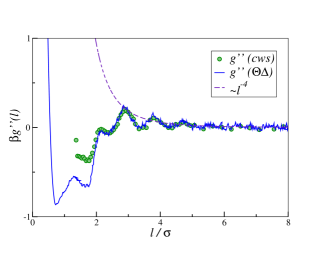
Figure 10: Plot of the second derivative of the interface potential as obtained from the capillary wave spectrum (symbols) and by numerical derivation of the thermodynamic interface potential of Fig. 5 (full lines). The dashed lines are expectations from the Hamaker model of Eq. (39) (results adapted from Ref.[45], correspond to the same model and temperature as in Fig. 4 and 5).

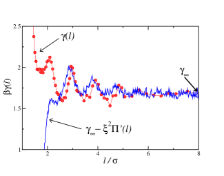
Figure 11: Plot of the film–height–dependent surface tension as obtained from the capillary wave spectrum of adsorbed films (symbols) of different height $\ell$. The lines are predictions from the model $\gamma_{\infty}-\xi_{\infty}^{2}\Pi^{\prime}(\ell)$, with $\Pi^{\prime}(\ell)$ as obtained from numerical derivatives of the disjoining pressure, Fig. 5 (results adapted from Ref.[45], correspond to the same model and temperature as in Fig. 4, 5 and 10.).

In our study, we simulated a large number of systems with average film thickness ranging from one to ten molecular diameters. For each configuration in a system, the Fourier components $\ell_{\mathbf{q}}$ of the film height profile were calculated and the thermal average $<|\ell_{\mathbf{q}}|^{2}>$ was obtained. We then performed a fit of the form:

$$\frac{k_{B}T}{A<|\ell_{\bf q}|^{2}>}=g^{\prime\prime}_{\rm cws}+\gamma_{\rm cws}\,q^{2}+\kappa_{\rm cws}\,q^{4}$$ (76)

By comparing with expectations from the capillary wave theory, Eq. (60), the coefficients $g^{\prime\prime}_{\rm cws}$, $\gamma_{\rm cws}$ and $\kappa_{cws}$, should provide estimates of $g^{\prime\prime}$, $\gamma_{\infty}$ and $\kappa$, respectively.

Figure 10 shows the zero order coefficients $g^{\prime\prime}_{\rm cws}$ as obtained from fits to the capillary wave spectrum (symbols). The results are compared to the second derivative of the interface potential described previously. The results indicate an excellent agreement between both independent estimates. Interestingly, the behavior is far from the asymptotic decay expected of the van der Waals forces, and rather, exhibits now a very strong oscillatory behavior that is revealing the layered structure of the adsorbed films that was apparent in the density profiles of Fig.4.

The second order coefficient of the film, $\gamma_{\rm cws}$ is, according to classical capillary wave theory, equal to the liquid–vapor surface tension, $\gamma_{\infty}$, in all the range of film thickness. This expectation is tested in Fig.11, where $\gamma_{\rm cws}$ is plotted as a function of $\ell$. Clearly, we find that results for thick films provide an accurate estimate of the surface tension as obtained independently for a free liquid vapor interface, marked as a thick arrow on the figure. However, as the films get thinner, an oscillatory behavior of $\gamma_{\rm cws}$ becomes apparent.

This behavior cannot possibly be explained in the framework of classical capillary wave theory, where the coefficient of the square gradient term is the liquid–vapor surface tension essentially by definition. The question is whether the interface potentials, or rather, the disjoining pressures that are actually measured experimentally are able to cope alone with all the film–height dependency required to describe the free energy of a rough interface as implied by the definition of the Interface Hamiltonian Model.

In the next section we will review recent theoretical work addressing this issue [45].

5 An improved capillary wave theory

Our simulation results of the capillary wave spectrum of adsorbed films confirm the expectations of the classical theory for thick films. However, the strong film–thick dependence of the surface tension that is observed for small $\ell$ clearly indicates room for improvement.

Recently, we have suggested that a film–thick–dependent surface tension may be explained by considering distortions of the intrinsic density profile beyond the mere interfacial translations that are considered in the classical theory [45].

The starting point is based on the seminal work of Fisher et al. on the nature of the short–range wetting transition [37, 38]. These authors attempted to derive the coarse–grained CWH from an underlying microscopic density functional of the square–gradient type. Their approach starts by seeking for a density profiles, $\rho(\mathbf{x};\Sigma)$ that extremalises the free energy functional subject to the constraint of a frozen capillary wave, $\ell(\mathbf{x})$, henceforth denoted as $\Sigma$ for short. The extremalised density profile, placed back into the underlying functional yields a formal expression for the free energy of the film of roughness $\Sigma$. This expression in then compared with the CWH, and the appropriate interface potential and surface tensions are identified.

Accordingly, let us assume that an adsorbed liquid film is frozen into a configuration of fixed roughness $\Sigma$, and let $\rho(\mathbf{r};\Sigma)$ be the corresponding average density. Within the double parabola approximation, seeking for a solution of $\rho(\mathbf{r};\Sigma)$ amounts to solving the Helmholtz equation, Eq. (13), subject to the constraint $\Sigma$.

The capillary waves impose weak transverse perturbations on the otherwise $z$ dependent density profile. Therefore, we suggest an expansion of $\rho(\mathbf{r};\Sigma)$ in transverse Fourier modes as trial solution [164]:

$$\rho(\mathbf{r};\Sigma)=\rho_{\infty}+\sum_{\mathbf{q}{}{}}\Delta\rho_{\mathbf{q}}(z;\mathbf{q}{}{})e^{i\mathbf{q}{}{}\cdot\mathbf{x}{}{}}$$ (77)

where, as in sections 2.1–2.3, $\rho_{\infty}$ denotes the asymptotic bulk density, which is either, $\rho_{l}$ to the left of $\ell(\mathbf{x})$ or $\rho_{v}$ to its right; while we will assume for the time being a symmetric fluid ($b_{l}=b_{v}=b$) for the sake of clarity. Later on, we will consider the more general solution that results when $b_{l}\neq b_{v}$.

Notice that this trial solution is of very general form. Particularly, being expressed in terms of Fourier coefficients, it suggests from the start that the density at a point $\mathbf{r}$ could depend, not just on the local properties at that point, but rather on the structure of the whole interface. The need to account for such nonlocal effects, which is absent in the theory of Fisher and Jin, has been strongly advocated by Parry and collaborators [39, 40, 44].

It is also worth mentioning that an expansion of the density profile in Fourier modes was previously employed by van Leeuwen and Sengers in their study of interfaces under gravity as described by the Square–Gradient density functional [165]. Relative to that work, however, we describe the local free energy explicitly in the double parabola approximation. This simplification will allow us to proceed without any further important approximation and obtain results in closed form that provide a more transparent interpretation.

Coming back to the solution of Eq. (77), we now apply the gradient operator twice on $\Delta\rho(\mathbf{r};\Sigma)$, followed by substitution into Eq. (13). It is then found that the transverse Fourier modes are the solution of an ordinary second order differential equation:

$$\frac{d^{2}\Delta\rho_{\mathbf{q}}(z)}{dz^{2}}-b_{q}^{2}\,\Delta\rho_{\mathbf{q}}(z)=\frac{\beta}{C_{\infty}}V_{\mathbf{q}}(z)$$ (78)

where $V_{\mathbf{q}}(z)$ are coefficients in a Fourier expansion of the external field, while $b_{q}$ is now a wave–vector dependent correlation length, promoting fast damping of small wavelength modes:

$$b_{q}^{2}=b_{\infty}^{2}+q^{2}$$ (79)

Clearly, Eq. (78) is formally equal to the equation for the independent branches of the planar liquid–vapor interface that we discussed in section 2.1, and actually becomes identical to Eq. (15) for the special case $q=0$. Accordingly, the formal solution for the eigenfunctions, $\Delta\rho_{\mathbf{q}}(z)$ is very similar and poses no difficulties. However, applying the boundary conditions for the general case is here far more involved.

Since the solutions of Eq. (78) for a structured adsorbed film that we are seeking is rather lengthy, and could obscure the generalities of the procedure, it will prove beneficial to consider first the capillary waves of a free liquid–vapor interface.

5.1 Liquid–vapor interface

For a liquid–vapor interface we can ignore the external field and obtain the eigenfunctions exactly as was done previously for the planar interface. Solving the homogeneous second order equation, followed by substitution of the Fourier modes $\Delta\rho_{\mathbf{q}{}{}}(z)$ into the trial solution, Eq. (77), we can write:

$$\rho_{\rm lv}({\bf r})=\rho_{\infty}+\sum_{\bf q}A_{\bf q}\,e^{\pm b_{q}z}e^{i{\bf q}\cdot{\bf x}}$$ (80)

with the understanding that the liquid branch is obtained by setting $\rho_{\infty}=\rho_{l}$ and $+b_{q}z$ as argument of the exponential; while the vapor branch corresponds to $\rho_{\infty}=\rho_{v}$ and $-b_{q}z$ in the exponential function (c.f. Eq. (18)). Furthermore, owing to the piecewise structure of the double parabola model, $\pm$ and $\mp$ signs will often appear in the expressions, and the understanding is that the top sign refers to the liquid branch, while the bottom sign corresponds to the vapor phase.

In order to obtain the Fourier coefficients of the rough liquid–vapor interface, $A_{\bf q}$, we evaluate $\rho({\bf r};\Sigma)$ at the boundary using the crossing criterion, such that the density at $z=\ell({\bf x})$ is fixed to some prescribed value $\rho_{1/2}$. The result is:

$$\rho_{1/2}=\rho_{\infty}+\sum_{\bf q}A_{\bf q}\,f_{\mathbf{q}}(\ell({\bf x}))\,e^{i{\bf q}\cdot{\bf x}}$$ (81)

where, for the sake of clarity, we have introduced the function $f_{\mathbf{q}}=e^{\pm b_{q}z}$, with plus sign for the liquid branch and minus sign for the vapor branch implied.

In order to proceed, we make a Taylor expansion of the right hand side up to second order in powers of $\delta\ell(\mathbf{x})=\ell(\mathbf{x})-\ell$:

$$\Delta\rho_{1/2}=\sum_{\bf q}A_{\bf q}\left\{f_{\mathbf{q}}(\ell)+f^{\prime}_{\mathbf{q}}(\ell)\,\delta\ell({\bf x})+\frac{1}{2}f^{\prime\prime}_{\mathbf{q}}(\ell)\,\delta\ell({\bf x})^{2}\right\}e^{i{\bf q}\cdot{\bf x}}$$ (82)

where, as in section 2.1, $\Delta\rho_{1/2}=\rho_{1/2}-\rho_{\infty}$.

It is now convenient to collect the $\mathbf{q}\neq 0$ coefficients, of which we retain terms up to linear order in $\delta\ell(\mathbf{x})$; separately from the $\mathbf{q}=0$ term of which we retain terms up to second order. We thus write:

$$\Delta\rho_{1/2}=S_{0}+S_{q}$$ (83)

with

$$S_{0}=A_{0}\left\{f_{0}(\ell)+f^{\prime}_{0}(\ell)\,\delta\ell({\bf x})+\frac{1}{2}f^{\prime\prime}_{0}(\ell)\delta\ell({\bf x})^{2}\right\}$$ (84)

and:

$$S_{q}=\sum_{{\bf q}\neq 0}A_{\bf q}\left\{f_{\mathbf{q}}(\ell)+f^{\prime}_{\mathbf{q}}(\ell)\,\delta\ell({\bf x})\right\}e^{i{\bf q}\cdot{\bf x}}$$ (85)

In order to obtain a relation for the coefficients $A_{{\bf q}\neq 0}$ we make a Fourier transform on both sides of Eq. (83), yielding:

$$\Delta\rho_{1/2}\,\delta({\bf q})=A_{0}\left[f_{0}(\ell)\,\delta({\bf q})+f^{\prime}_{0}(\ell)\,\delta\ell_{\bf q}\right]+\sum_{{\bf q}^{\prime}\neq 0}A_{\bf q^{\prime}}f_{\mathbf{q}^{\prime}}(\ell)\,\delta({\bf q}^{\prime}-{\bf q})$$ (86)

where we have neglected the last term in both $S_{0}$ and $S_{q}$. For ${\bf q}\neq 0$, all terms with a Dirac delta vanish, and we are left with a relation between $A_{\bf q}$ and $A_{0}$:

$$A_{\bf q}f_{\mathbf{q}}(\ell)=-A_{0}\,f^{\prime}_{0}(\ell)\,\delta\ell_{\bf q}$$ (87)

For the ${\bf q}=0$ term, we only need to make an unweighted lateral average on both sides of Eq. (83), which, retaining all terms in $S_{0}$ and $S_{q}$, leads to the following equality:

$$\Delta\rho_{1/2}=A_{0}\left\{f_{0}(\ell)+\frac{1}{2}f^{\prime\prime}_{0}(\ell)\sum_{\mathbf{q}}\delta\ell_{\bf q}\delta\ell_{-{\bf q}}\right\}+\sum_{\bf q}A_{\bf q}\,f^{\prime}_{\mathbf{q}}(\ell)\,\delta\ell_{-{\bf q}}$$ (88)

Here, we have invoked once more Plancherel’s theorem in order to write the second term inside the brackets in terms of $\delta\ell_{\bf q}\delta\ell_{-{\bf q}}$.

We can now eliminate the $A_{\mathbf{q}}$ coefficients of the above result using Eq. (87) and obtain a closed expression for $A_{0}$ in terms of $\delta\ell_{\bf q}$:

$$\Delta\rho_{1/2}=A_{0}\,f_{0}(\ell)\left\{1+\sum_{\mathbf{q}}\left[\frac{1}{2}\frac{f^{\prime\prime}_{0}(\ell)}{f_{0}(\ell)}-\frac{f^{\prime}_{0}(\ell)}{f_{0}(\ell)}\frac{f^{\prime}_{\mathbf{q}}(\ell)}{f_{\mathbf{q}}(\ell)}\right]\delta\ell_{\bf q}\delta\ell_{-{\bf q}}\right\}$$ (89)

Using the results of the last two paragraphs, we readily obtain the following expression for the coefficients of the series:

$$A_{0}=\Delta\rho_{1/2}\,f_{0}^{-1}(\ell)\left\{1-\sum_{\bf q}\left[\frac{1}{2}\frac{f^{\prime\prime}_{0}(\ell)}{f_{0}(\ell)}-\frac{f^{\prime}_{0}(\ell)}{f_{0}(\ell)}\frac{f^{\prime}_{\mathbf{q}}(\ell)}{f_{\mathbf{q}}(\ell)}\right]\delta\ell_{\bf q}\delta\ell_{-{\bf q}}\right\}$$ (90)

$$A_{\bf q}=-\Delta\rho_{1/2}\,\frac{f^{\prime}_{0}(\ell)}{f_{0}(\ell)\,f_{\mathbf{q}}(\ell)}\,\delta\ell_{\bf q}$$ (91)

We can now replace the coefficients back into Eq. (80), and obtain the sought equation for the liquid–vapor density profile of a rough interface:

$$\begin{array}[]{lll}\rho({\bf r};\Sigma)&=&\rho_{\pi}(z;\ell)+\frac{1}{2}\Delta\rho_{1/2}e^{\pm b(z-\ell)}\sum_{\bf q}\left[b^{2}+q^{2}\right]\delta\ell_{\bf q}\delta\ell_{-{\bf q}}\\ &&\\ &&\mp b\,\Delta\rho_{1/2}\sum_{\bf q}e^{\pm b_{q}(z-\ell)}\,\delta\ell_{\bf q}\,e^{i{\bf q}\cdot{\bf x}}\end{array}$$ (92)

where $\rho_{\pi}(z;\ell)$ here stands for the intrinsic density profile of a liquid–vapor interface in the double parabola approximation, Eq. (20). This result already without any further elaboration provides us with a great deal of insight on how capillary–waves modify the structure of an interface. For the time being, we briefly mention here just a few:

• The perturbed density profile $\rho({\mathbf{r}};\Sigma)$, has a leading order contribution equal to the intrinsic density profile of the planar interface.

• To linear order in the perturbation, the capillary waves provoke an additional dependence on the transverse direction, $\mathbf{x}$. Contrary to expectations from the classical theory, however, the decay of this perturbation is not merely given by the inverse correlation length, $b$. Rather, short wavelength perturbations decay at a faster, wave–vector dependent rate, $b_{q}$.

• To second order in the perturbation, the capillary waves result in an additional $z$ dependent contribution to the density profile which is responsible for the capillary wave broadening. Following expectations from the classical theory, the broadening depends on the average squared amplitude of the capillary perturbation, $\sum|\delta\ell_{q}|^{2}$ (c.f. Eq. (62)). However, as first noted in [45], there is an additional capillary wave broadening mechanism of order $\sum|q\,\delta\ell_{q}|^{2}$ not included in the classical theory.

We postpone further discussion of the implications to a later section, and consider now the density profile of an adsorbed film.

5.2 Adsorbed films

Having studied the case of a free liquid–vapor interface, let us now consider the role of capillary waves on the structure of an adsorbed film. Clearly, by definition the capillary waves propagate at the liquid–vapor interface, so the question is, to what extent do they penetrate and distort the structure of the layered film. The results of Fig.9, are quite revealing in this regard, and show that, despite the obvious broadening of the density profile at the liquid–vapor interface, the layering structure of the adsorbed liquid remains essentially unchanged as the system size increases, exhibiting no sign of broadening what so ever. This suggests that we can employ the superposition approximation of section 2.3, with all of the capillary wave effects lumped into the liquid–vapor density profile. Accordingly, we consider solutions of the form (c.f. Eq. (34)):

$$\rho(\mathbf{r};\Sigma)=[1+h_{\rm wl}(z)]\,\rho_{\rm lv}(\mathbf{r};\Sigma)$$ (93)

where, at this stage, $\rho_{\rm lv}(\mathbf{r};\Sigma)$ adopts the general form for the solution of the Helmholtz equation, as given in Eq. (80).

In order to look for the coefficients of the above equation, we employ again the crossing criterion, and set:

$$\rho_{1/2}=\left[1+h_{\rm wl}(\ell(\mathbf{x}))\right]\times\left[\rho_{\infty}+\sum_{\bf q}A_{\bf q}e^{\pm b_{q}\ell({\bf x})}e^{i{\bf q}\cdot{\bf x}}\right]$$ (94)

Calculations are now much more lengthy than before, but proceed exactly in the same manner. i.e, a Taylor expansion in powers of $\delta\ell$ is performed, the resulting expressions are Fourier transformed, and the set of linear equations is solved. We omit the lengthy details here and write the final solution, which can be given in compact form in terms of an intrinsic density profile and recovers the result for the liquid–vapor interface (c.f. Eq. (92)) when $h_{\rm wl}(z)=0$:

$$\begin{array}[]{lll}\rho({\bf r};\Sigma)&=&\rho_{\pi}(z;\ell)+\frac{1}{2}\sum_{\bf q}\left[\frac{d^{2}\rho_{\pi}(z;\ell)}{d\ell^{2}}\mp\frac{d\rho_{\pi}(z;\ell)}{d\ell}\frac{q^{2}}{b}\right]|\delta\ell_{\bf q}|^{2}\\ &&\\ &&+\frac{d\rho_{\pi}(\ell;\ell)}{d\ell}\sum_{\bf q}\delta\ell_{\bf q}\;(1+h_{\rm wl}(z))e^{\pm b_{q}(z-\ell)}e^{i{\bf q}\cdot{\bf x}}\end{array}$$ (95)

where now, the intrinsic density profile is that given for planar adsorbed films in section 2.3, Eq. (35).

This equation shares the same qualitative implications that where found for the free liquid–vapor interface. Of particular interest is the laterally averaged density profile, which is immediately recovered from the above result as the $q=0$ Fourier coefficient:

$$\rho(z;\Sigma)=\rho_{\pi}(z;\ell)+\frac{1}{2}\sum_{\bf q}\left[\frac{d^{2}\rho_{\pi}(z;\ell)}{d\ell^{2}}\mp\frac{d\rho_{\pi}(z;\ell)}{d\ell}\frac{q^{2}}{b}\right]|\delta\ell_{\bf q}|^{2}$$ (96)

if we now recall that $\sum_{\bf q}|\delta\ell_{\bf q}|^{2}=\langle\delta\ell^{2}\rangle_{\mathbf{x}}$, while $\sum_{\bf q}|q\delta\ell_{\bf q}|^{2}=\langle\nabla\ell^{2}\rangle_{\mathbf{x}}$, we see that the rough interface profile may be written as an expansion in powers of the squared amplitudes and gradient:

$$\rho(z;\Sigma)=\rho_{\pi}(z;\ell)+\frac{1}{2}\frac{d^{2}\rho_{\pi}(z;\ell)}{d\ell^{2}}\langle\delta\ell^{2}\rangle_{\mathbf{x}}\mp\frac{1}{2}\frac{d\rho_{\pi}(z;\ell)}{d\ell}\langle(\nabla\ell)^{2}\rangle_{\mathbf{x}}$$ (97)

where $\langle\rangle_{\mathbf{x}}$ denotes the unweighted lateral average $1/A\int d\mathbf{x}$.

In order to work out the implications of this equation more transparently, it is convenient to consider the limit of thick adsorbed films, where the wall correlations have essentially died out, so that $h_{wl}(z)=0$. In that case, the liquid–vapor interface is unperturbed by the substrate and is equal to the free liquid–vapor interface. Using now Eq. (18), it can be readily seen that $d^{2}\rho_{\pi}(z)/d\ell^{2}$ and $\mp bd\rho_{\pi}(z)/d\ell$ become equal within the double parabola approximation, and the capillary wave perturbed density profile becomes:

$$\rho(z;\Sigma)=\rho_{\pi}(z;\ell)+\frac{1}{2}\frac{d^{2}\rho_{\pi}(z;\ell)}{d\ell^{2}}\left\{\langle\delta\ell^{2}\rangle_{\mathbf{x}}+\xi^{2}_{\infty}\langle(\nabla\ell)^{2}\rangle_{\mathbf{x}}\right\}$$ (98)

Notice that this equation is similar to the classical result for the density broadening due to capillary waves (c.f. Eq. (62)), however, an extra term of order square gradient as identified in Ref.[45] for the first time is present.

5.3 Capillary wave spectrum

Having obtained the density profile consistent with the constraint $\Sigma$, we can now plug back $\rho({\bf r};\Sigma)$ into the free energy functional in order to estimate the free energy of the assumed capillary wave fluctuation. In practice, because we are interested in films subject to long–range van der Waals forces, it will suffice, as was the case in section 2.4, to evaluate the dominant external field contribution. Luckily, since we are assuming an external field that only depends on the perpendicular direction, only the laterally averaged density profile is required. Hence, using Eq. (98) into Eq. (37), readily yields:

$$g_{V}(\Sigma)=g_{V}(\ell)+\frac{1}{2}\left\{\langle\delta\ell^{2}\rangle_{\mathbf{x}}+\xi^{2}_{\infty}\langle(\nabla\ell)^{2}\rangle_{\mathbf{x}}\right\}\int\frac{d^{2}\rho_{\pi}(z)}{d\ell^{2}}V(z)dz$$ (99)

In order to obtain the overall free energy of the perturbation, we now replace this equation into Eq. (43), using $g_{V}(\Sigma)$ as an estimate for the full $g(\Sigma)$. Comparing the result with Eq. (44), we see that the term of order $\langle\delta\ell^{2}\rangle_{\mathbf{x}}$ can be readily identified with $g^{\prime\prime}_{V}(\ell)$. However, the term of order $\langle\nabla\ell^{2}\rangle_{\mathbf{x}}$ that is proportional to the surface area of the capillary wave, can only be incorporated as an effective contribution to the surface tension. Whence, we can write, in a more compact form:

$$g_{V}(\Sigma)=g_{V}(\ell)+\frac{1}{2}g_{V}^{\prime\prime}(\ell)\langle\delta\ell^{2}\rangle_{\mathbf{x}}+\Delta\gamma(\ell)\langle\nabla\ell^{2}\rangle_{\mathbf{x}}$$ (100)

where the coefficient $g_{V}^{\prime\prime}(\ell)$ is given exclusively in terms of the intrinsic density profile:

$$g_{V}^{\prime\prime}(\ell)=\int\frac{d^{2}\rho_{\pi}(z)}{d\ell^{2}}V(z)dz$$ (101)

while the $\ell$ dependent contribution to the surface tension is [45]:

$$\Delta\gamma(\ell)=\xi^{2}_{\infty}\,g_{V}^{\prime\prime}(\ell)$$ (102)

Substitution of Eq. (100) into Eq. (43), and transforming fluctuations of $\ell(\mathbf{x})$ as usual, we finally obtain, for the Fourier transformed Hamiltonian, the following result:

$$H[\Sigma]=Ag(\ell)+\frac{1}{2}\sum_{\mathbf{q}}[g^{\prime\prime}(\ell)+(\gamma_{\infty}+\Delta\gamma(\ell))\,q^{2}]\delta\ell_{\mathbf{q}}\delta\ell_{-\mathbf{q}}$$ (103)

Comparing this result with Eq. (47), we readily see that the consistent statistical thermodynamic treatment of the capillary wave Hamiltonian provides a free energy very much in agreement with the phenomenological classical capillary wave theory. The difference is, however, that the square–gradient coefficient, corresponding to $\gamma_{\infty}$ in the classical theory, is augmented with an extra $\ell$ dependent contribution $\Delta\gamma(\ell)$.

We can now readily obtain the spectrum of fluctuations consistent with Eq. (103), by following the same procedure discussed earlier (section 3.1). The result is:

$$\frac{k_{B}T}{A\langle|\ell_{\mathbf{q}}|^{2}\rangle}=g^{\prime\prime}(\ell)+(\gamma_{\infty}+\Delta\gamma(\ell))q^{2}$$ (104)

This equation shows that the $q^{2}$ coefficient of the CWS is not just $\gamma_{\infty}$ as implied by the classical theory, Eq. (51), but rather, picks up an additional $\ell$ dependent contribution, which, under some simplifying assumptions follows Eq. (102).

Since both $g^{\prime\prime}(\ell)$ and $\gamma(\ell)$ are available from that study of Ref.[45], and $g^{\prime\prime}(\ell)$ is essentially dominated by $g_{V}^{\prime\prime}(\ell)$, is suffices to employ $\xi^{2}_{\infty}$ as an empirical parameter in order to test the expectation of the above equation, namely, that the coefficient of order $q^{2}$ in the CWS, obeys $\gamma(\ell)=\gamma_{\infty}+\xi^{2}_{\infty}g^{\prime\prime}(\ell)$. The result of the comparison, depicted in Fig.11, shows clearly a strong correlation between $\gamma(\ell)$ and $g^{\prime\prime}(\ell)$, in all the range where $g^{\prime\prime}(\ell)$ is dominated by the long–range forces. The agreement clearly breaks down below two molecular diameters but in that regime the short range forces become relevant and Eq. (102) need not hold any longer.

Particularizing Eq. (103) to the specific case of an algebraically decaying potential, we recover a result obtained previously from the nonlocal theory of interfaces [44]. That theory has been largely applied to the study of short range wetting, but its implications as regards to capillary wave broadening, and the effect of long range forces have hardly been considered [43, 44]. An effort is still needed to assess to what extent are both approaches equivalent.

Before closing, let us mention that, if we explicitly consider the asymmetry of the liquid and vapor phases, $\Delta\gamma(\ell)$ then picks up additional terms of order $g^{\prime}(\ell)$ which vanish in the limit of a symmetrical fluid, as noted previously [44]. A result exact for the double parabola model up to linear order in the asymmetry is:

$$\Delta\gamma(\ell)=\frac{1}{2}(\xi_{l}^{2}+\xi_{v}^{2})g^{\prime\prime}(\ell)-\frac{1}{4}(\xi_{l}^{2}-\xi_{v}^{2})(\frac{1}{\xi_{l}}+\frac{1}{\xi_{v}})g^{\prime}(\ell)+O((\xi_{l}^{2}-\xi_{v}^{2})^{2})$$ (105)

According to the analysis performed in [45], terms governed by $g^{\prime}(\ell)$ do not yield any significant improvement for the model of Argon on carbon dioxide, indicating a small role of the asymmetry even at such low temperature.

5.4 Capillary wave broadening

Another important implication of the theoretical analysis of Ref.[45] refers to the roughening of the average interface profile as described by Eq. (97) and Eq. (98). Clearly, the first two terms on the right hand side of Eq. (97), are exactly as predicted by the classical capillary wave theory for an expansion of $\rho(\mathbf{r};\Sigma)$ about $\ell$ (c.f. Eq. (62)), but the third term implies a contribution of order square–gradient to the capillary wave broadening, that had not been identified previously. Physically, this contribution implies that the capillary waves do not merely propagate by translation of the original perturbation, $\ell(\mathbf{x})$, but rather, are distorted due to curvature of the interface, and lead to iso–density lines that are no longer parallel.

In order to assess the extent of the square–gradient contribution it is more convenient to consider the simplified Eq. (98). Comparing that equation with Eq. (62), shows that the the combined contributions of translation and distortion to capillary wave broadening may be interpreted as an effective translation enhanced by terms of order square–gradient. Whence, the combined effects may be lumped into a single roughening parameter $\Delta^{2}_{\rm cw}$, as:

$$\begin{array}[]{ccc}\Delta^{2}_{\rm cw}&=&\langle\delta\ell^{2}\rangle+\xi^{2}_{\infty}\langle(\nabla\ell)^{2}\rangle\\ &&\\ &=&\sum_{\mathbf{q}}(1+\xi^{2}_{\infty}q^{2})\langle|\delta\ell_{\mathbf{q}}|^{2}\rangle\end{array}$$ (106)

where the Fourier amplitudes, $\delta\ell_{\mathbf{q}}$ are given by Eq. (104). This sum may be transformed into an integral as for the classical theory. For the sake of generality, however, we extend the result of Eq. (104), by adding the next to leading order correction, $\kappa\,q^{4}$ to the denominator of $\langle|\delta\ell_{\mathbf{q}}|^{2}\rangle$, as implied by the Helfrich Hamiltonian and discussed at length by Mecke [97] (c.f. Eq. (60)). Performing the integral to leading order in $\kappa$, we obtain an expression in real algebra that smoothly transforms into the classical result, Eq. (56):

$$\Delta_{\rm cw}^{2}=\Delta_{\rm\gamma}^{2}+\Delta_{\rm\kappa}^{2}$$ (107)

with

$$\Delta_{\gamma}^{2}=\frac{k_{B}T}{4\pi\gamma(\ell)}\left[\frac{\xi^{2}_{\parallel}-\xi^{2}_{\infty}}{\xi^{2}_{\parallel}-2\xi^{2}_{\rm R}}\right]\ln\left(\frac{1+\xi_{\parallel}^{2}q_{\rm max}^{2}}{1+\xi_{\parallel}^{2}q_{\rm min}^{2}}\right)$$ (108)

and

$$\Delta_{\kappa}^{2}=\frac{k_{B}T}{4\pi}\frac{\xi^{2}_{\infty}}{\kappa}\left[\frac{\xi_{\parallel}^{2}-(1+\xi_{\parallel}^{2}/\xi^{2}_{\infty})\xi^{2}_{\rm R}}{\xi_{\parallel}^{2}-2\xi^{2}_{\rm R}}\right]\ln\left(\frac{\xi_{\parallel}^{2}-(1-\xi_{\parallel}^{2}q_{\rm max}^{2})\xi^{2}_{\rm R}}{\xi_{\parallel}^{2}-(1-\xi_{\parallel}^{2}q_{\rm min}^{2})\xi^{2}_{\rm R}}\right)$$ (109)

In these equations, $\gamma(\ell)$ refers to the $\ell$ dependent quantity $\gamma(\ell)=\gamma_{\infty}+\xi_{\infty}^{2}g^{\prime\prime}(\ell)$ defined previously; $\xi_{\infty}$ is the bulk correlation length; a sort of bending correlation length $\xi_{\rm R}^{2}=\kappa/\gamma$ emerges naturally; while the parallel correlation length is now given as:

$$\begin{array}[]{ccc}\xi^{2}_{\parallel}&=&\frac{\gamma(\ell)}{g^{\prime\prime}(\ell)}\\ &&\\ &=&\frac{\gamma_{\infty}}{g^{\prime\prime}(\ell)}+\xi_{\infty}^{2}\end{array}$$ (110)

Note that Eq. (107) was written in terms of the two contributions $\Delta_{\gamma}$ and $\Delta_{\kappa}$ for the sake of brevity, but physically, it is more relevant to write

$$\Delta^{2}_{\rm cw}=\Delta^{2}_{\rm tras}+\Delta^{2}_{\rm dis}$$ (111)

where $\Delta^{2}_{\rm tras}=\langle\delta\ell^{2}\rangle$ is the interface translation roughening, while $\Delta^{2}_{\rm dis}=\xi^{2}_{\infty}\langle(\nabla\ell)^{2}\rangle$ is the interface distortion roughening. These contributions may be readily recognized from Eq. (108)–Eq. (109) by noticing that $\Delta^{2}_{\rm dis}$ has a linear prefactor of order $\xi_{\infty}^{2}$.

The picture that emerges from these equations is that the roughness of an interface as measured from experiments is, for the most general case, a very subtle phenomenon involving bulk and interface properties as well as surface interactions. It is relevant to recall in this context, that the above result, actually, was obtained via the simplifying assumption of i) a symmetric fluid, and ii) the liquid–vapor interface unaffected by the field.

In practice, the expression obtained here does not upset the good experimental agreement of the classical theory in the low field limit. Indeed, assuming $\xi_{\parallel}$ is larger than the system size, $\xi_{\parallel}q_{\rm min}\gg 1$, and neglecting $\xi_{R}$, we find:

$$\Delta^{2}_{cw}=\frac{k_{B}T}{2\pi\gamma_{\infty}}\left[\ln\left(\frac{q_{\rm max}}{q_{\rm min}}\right)+\frac{1}{2}\xi_{\infty}^{2}q_{\rm max}^{2}\right]$$ (112)

whence, the distortion contribution to the interface is a constant and does not upset the $\ln L$ dependence observed experimentally. Presumably, the extra term could be tested experimentally by performing scattering experiments with different instrumental cutoffs.

If, however, we consider the strong field limit, we find that indeed, because of the $\ell$ dependence of the surface tension, the predicted roughness exhibits important differences with the classical theory, already under the simplifying assumption of vanishing $\xi_{R}^{2}$:

$$\Delta^{2}_{cw}=\frac{k_{B}T}{2\pi\gamma(\ell)}\left[\left(1-\frac{\xi_{\infty}^{2}}{\xi_{\parallel}^{2}}\right)\ln\left(\xi_{\parallel}q_{\rm max}\right)+\frac{1}{2}\xi_{\infty}^{2}q_{\rm max}^{2}\right]$$ (113)

Particularly, this equation predicts a sharper increase of the roughness towards the low field limit than the classical theory, and such behavior does indeed conform qualitatively to some of the experimental findings [166, 115, 116].

The results above await verification, but it is interesting to point out that already some authors have noticed that their results could be better described with a film–height dependent surface tension [86, 166, 115, 116].

Particularly relevant here is the work by Wang et al. [166], who studied thin polymer films at conditions where the bulk fluid exhibits liquid like behavior. Unexpectedly, the specular and diffuse x–ray scattering experiments performed could not be described simultaneously from the classical capillary wave theory of section 3.2. On the one hand, their diffuse scattering experiments could only be described with an enhanced surface tension. On the other hand, such enhancement would result in interfacial roughness much smaller than implied by their specular reflectivity data. The authors reconciled these conflicting observations by hypothesizing a strong viscoelastic behavior of the polymer films, implying some degree of “glassification” as a result of confinement. However, Eq. (113) shows that, due to the additional contribution $\xi_{\infty}^{2}q_{\rm max}^{2}$, an enhanced surface tension is actually compatible with an enhanced roughness, and could also serve as an explanation for the observed behavior.

It is tempting to apply the result above to the case of a fluid–fluid interface subject to gravity. As the fluid approaches the critical point, $\xi_{\parallel}$ approaches $\xi_{\infty}$ (c.f. Eq. (110)). Whence, according to Eq. (113), the logarithmic contributions of translation and distortion roughening cancel each other exactly, and only an ultraviolet cutoff term approaching $q_{\rm max}^{2}$ survives. This result is in agreement with theoretical estimates by van Leeuwen and Sengers, who considered the role of capillary wave translations on the Fisk–Widom intrinsic density profile and predicted a negligible roughening at criticality [165]. Interpertations based on Eq. (113) must be taken with some caution, however, since our approach assumes the external field does not perturb the intrinsic density profile. As is clear from Eq. (33), this is a reasonable approximation for an incompressible fluid, but breaks down at criticality because of the diverging compressibility.

5.5 Discussion

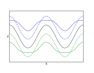
Figure 12: Sketch with iso–density lines representing a monochromatic capillary wave perturbation. The black line is the initial perturbation as imposed by the crossing criterion, satisfying $\rho(\mathbf{x};z=\ell(\mathbf{x}))=\rho_{1/2}$. The blue lines (top) correspond to iso-density curves inside the vapor phase with $\rho=\frac{1}{2}(\rho_{v}-\rho_{1/2})$, while the green curves (bottom) correspond to iso-density curves in the liquid phase, $\rho=\frac{1}{2}(\rho_{l}-\rho_{1/2})$. Full lines are predictions from Eq. (114), while dashed lines are the classical theory in the double parabola approximation (i.e., Eq. (114) with gradient and Laplacian terms ignored). The monochromatic perturbation has wavelength of five and amplitude 9/10 in units of the correlation length.

In this section we will discuss some physical implications of the general result, Eq. (95), leading naturally to the identification of the film–height dependent surface tension.

In that equation, the $q=0$ contribution of $\rho(\mathbf{r};\Sigma)$ features terms of order $|\delta\ell_{\mathbf{q}}|^{2}$ and $|q\,\delta\ell_{\mathbf{q}}|^{2}$, while, due to mathematical difficulties, $q\neq 0$ Fourier coefficients are given only to order $\delta\ell_{\mathbf{q}}$. The $q=0$ mode of Eq. (95) is written in convenient form in Eq. (97). There, it is clear that, apart from the intrinsic density profile, there appear terms that are lateral averages of $\delta\ell(\mathbf{x})$ and $(\nabla\ell)^{2}$. Since the $q=0$ mode in a Fourier expansion is essentially an unweighted lateral–average of the full solution, we conclude that $\rho(\mathbf{r};\Sigma)$ must feature terms that are of order $\delta\ell(\mathbf{x})^{2}$, and $(\nabla\ell(\mathbf{x}))^{2}$ that are missing in Eq. (95) because of the truncation to order $\delta\ell_{\mathbf{q}}$ in the $q\neq 0$ Fourier modes.

A further important mathematical feature of the solution may be noticed by expanding the exponential function of Eq. (95), which immediately shows that $\rho(\mathbf{r};\Sigma)$ also features terms of order $q^{2}\,\delta\ell_{\mathbf{q}}$ which can be immediately related to the Laplacian, $\nabla^{2}\ell(\mathbf{x})$.

Thus, to the order that is implied in Eq. (95), we can conclude that $\rho(\mathbf{r};\Sigma)$ may be expressed as a function of $\delta\ell(\mathbf{x})$, $[\nabla\ell(\mathbf{x})]^{2}$ and $\nabla^{2}\ell(\mathbf{x})$. Whence, the strong nonlocality that is potentially implied in the trial solution of Eq. (77), is to this order a “weak” nonlocality, such that $\rho(\mathbf{r};\Sigma)$ may be expressed as a local function of the interface displacement, squared gradient and Laplacian. This feature of the solutions of the Helmholtz equation were already noticed some time ago [38], but not explored any further. The weak nonlocality implied here, however, provides a much more complex behavior than the classical theory, where $\rho(\mathbf{r};\Sigma)$ is only a local function of $\delta\ell(\mathbf{x})$.

Heuristically, we can suggest the following extended local form for the rough liquid–vapor density profile $\rho(\mathbf{r};\Sigma)$ in the double parabola approximation [167]:

$$\rho(\mathbf{r};\Sigma))=\left\{\begin{array}[]{ll}\rho_{l}-\Delta\rho_{1/2}e^{(L_{\bf x}+b_{\bf x})(z-\ell)}&z<\ell(\mathbf{x})\\ &\\ \rho_{v}+\Delta\rho_{1/2}e^{(L_{\bf x}-b_{\bf x})(z-\ell)}&z>\ell(\mathbf{x})\end{array}\right.$$ (114)

where $L_{\bf x}=\frac{1}{2}(1+(\nabla\ell)^{2})^{-1}\nabla^{2}\ell$ and

$$b_{\bf x}=\frac{\sqrt{b^{2}+b^{2}(\nabla\ell)^{2}+\frac{1}{4}(\nabla^{2}\ell})^{2}}{1+(\nabla\ell)^{2}}$$ (115)

is a local, curvature dependent correlation length that plays the same role as $b_{q}$ in the Fourier mode theory. The motivation for this result may be grasped intuitively for the special case of a film profile $\ell(\mathbf{x})$ locally exhibiting finite gradient but zero curvature $\nabla^{2}\ell(\mathbf{x})=0$. In that case, Eq. (114) is transformed into a function $\rho_{\pi}(h(z,\mathbf{x}))$ of the single variable:

$$h=\frac{z-\ell(\mathbf{x})}{\sqrt{1+(\nabla\ell)^{2}}}$$ (116)

whence, in contrast with the classical theory, which assumes vertical interface translations $z\to z-\ell(\mathbf{x})$ of the profile, the above result considers the density of the inclined profile as given by the shortest (perpendicular) distance to the interface (rather than the vertical distance). This ansatz, which seems rather natural on physical grounds, has been invoked occasionally in improved capillary wave models for the description of the liquid–vapor interface [85, 109].

In order to compare the result of Eq. (114) with that of Eq. (95), we expand $\rho(\mathbf{r};\Sigma))=f(\mathbf{r};\delta\ell,(\nabla\ell)^{2},\nabla^{2}\ell)$ about the planar interface, yielding:

$$\begin{array}[]{ccc}\rho(\mathbf{r};\Sigma))&=&\rho_{\pi}(z)+\frac{d\rho_{\pi}}{d\ell}\delta\ell(\mathbf{x})\mp\frac{1}{2}\frac{z-\ell_{\pi}}{b}\frac{d\rho_{\pi}}{d\ell}\nabla^{2}\ell(\mathbf{x})+\frac{1}{2}(z-\ell_{\pi})\frac{d\rho_{\pi}}{d\ell}(\nabla\ell(\mathbf{x}))^{2}\\ &&\\ &&+\frac{1}{2}\frac{d^{2}\rho_{\pi}}{d\ell^{2}}\delta\ell(\mathbf{x})^{2}+O(\delta\ell\nabla^{2}\ell,\delta\ell^{3},(\nabla\ell)^{2},(\nabla^{2}\ell)^{2})\end{array}$$ (117)

The first two terms of Eq. (114) recover exactly the Fisher–Jin theory of short–range wetting [37, 38]. Since upon performing a lateral average, the linear term in $\delta\ell$ vanishes, it is clear that the Fisher–Jin result does not give capillary wave broadening at all, and can therefore not possibly yield the film–height surface tension arising from the external field contribution. That is not a problem in the study of short–range wetting, where the field is of zero range, but is very relevant in practical applications discussed here.

A similar expansion performed for Eq. (95) for the case of a liquid–vapor interface ($h_{\rm wl}(z)=0$) is identical to this equation, except for the $\mp\frac{d\rho_{\pi}}{d\ell}$ term of Eq. (95), which here transforms the $\mp$ sign inversion between branches somewhat more naturally as $(z-\ell_{\pi})\frac{d\rho_{\pi}}{d\ell}$. Whence, to the order of approximation that is implied in Eq. (95), Eq. (114) seems a rather reasonable guess. An advantage of the heuristic approach is that the crossing criterion is obeyed by construction for whatever large interfacial displacement. This is not the case of Eq. (95), because the boundary condition can only be solved in practice by performing an expansion in small powers of $\delta\ell$.

The above equation can now be laterally averaged, providing the capillary wave broadened profile. Since the terms linear in the interface displacement and Laplacian vanish, we are left with:

$$\rho(z;\Sigma)=\rho_{\pi}(z)+\frac{1}{2}\frac{d^{2}\rho_{\pi}}{d\ell^{2}}\langle\delta\ell^{2}\rangle_{\mathbf{x}}+\frac{1}{2}(z-\ell_{\pi})\frac{d\rho_{\pi}}{d\ell}\langle(\nabla\ell)^{2}\rangle_{\mathbf{x}}$$ (118)

a result that is again of very similar form to Eq. (97).

The picture that emerges from this discussion is that the addition of contributions in the gradient and Laplacian distort the density profile of the planar film beyond mere interface translations, compressing or relaxing iso–density curves parallel to the capillary wave perturbation. This is illustrated in Fig.12, which shows schematically iso–density curves for the classical theory, compared with results from $Eq.~{}(\ref{eq:dpm})$. In the classical theory, the perturbation propagates parallel to the initial wave front imposed by the crossing criterion. In the modified theory, however, iso–density lines at one phase (say the vapor phase) detach the original wave front for perturbations protruding into the liquid, while they approach the wave front when the liquid phase protrudes into the vapor (and likewise for iso-density lines in the liquid phase). Whence, relative to the classical theory, the perturbation is relaxed faster in a phase that is receding in favor of the opposite (whence, contributing to a smaller broadening than implied in the classical theory); but relaxes slower when it is that phase which protrudes into the opposite (therefore, contributing to a stronger broadening than predicted by the classical theory). Subsequent calculations in the framework of the nonlocal theory [168] are consistent with our results, Ref.[45, 167].

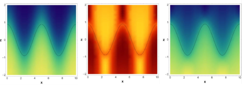
Figure 13: Density plots of a monochromatic capillary perturbation as described by the classical (left), and the improved capillary wave theories (right). Dark blue corresponds to the bulk vapor density (top phase), dark yellow to the bulk liquid density (bottom phase), green values correspond to intermediate densities. The figure in the center shows differences between the improved and the classical theories, with yellow indicating positive differences, red color negative differences, and orange, no difference. The perturbation is the same as explained in the caption of Fig.12.

On laterally averaging these two opposing effects, the net contribution is that of an increased capillary wave broadening, as implied in Eq. (97) and Eq. (118). Figure 13 illustrates this effect for the simple monochromatic perturbation already considered previously in Fig.12. The color code which is darker for densities close to the bulk phase, shows that the relaxation is fast in the phase receding from the equimolar surface, but is slow in the phase protruding into the equimolar surface (this can be best seen by considering the color code along a horizontal line close to the top or bottom of the figure). In order to illustrate the difference more clear, the central panel of the figure shows the density differences between the improved and the classical theories. A dominant positive region in the low density phase and an oppositely dominant negative region in the high density phase indicate enhanced capillary wave broadening.

6 Conclusions and outlook

The most important outcome of this review is an improved form of the Interfacial Hamiltonian Model Eq. (1) employed in surface thermodynamics for the study of adsorbed condensates. According to our recent findings, a better description of thin films of height $\ell(\mathbf{x})$ subject to the effect of a finite disjoining pressure in the small gradient regime is:

$$H[\ell(\mathbf{x})]=\int\left\{g(\ell)+\frac{1}{2}\gamma(\ell)[\nabla\ell]^{2}\right\}d\mathbf{x}$$ (119)

where $\gamma(\ell)$ is a film–height dependent surface tension that asymptotically recovers the result of a free liquid–vapor interface, $\gamma_{\infty}$. To leading order, it is found that [45]:

$$\gamma(\ell)=\gamma_{\infty}-\xi_{\infty}^{2}\frac{d\Pi(\ell)}{d\ell}$$ (120)

where $\xi_{\infty}$ is the bulk correlation length. In the limit where the square gradient coefficient is a constant equal to the surface tension, the extremum of the Interface Hamiltonian provides a generalized or augmented Young–Laplace equation that is extensively employed to determine the equilibrium properties of condensates [20, 22, 16, 23]. The explicit $\ell$ dependence of $\gamma(\ell)$, however, shows that the stationary condition of the Interface Hamiltonian may be more complicated than suggested by the augmented Young–Laplace equation.

The above result should be accurate at least in the small curvature regime, which, for the case of sessile drops may correspond to contact angles as large as 30 degrees [169]. The accuracy may be also limited to a range of film heights where the effect of an external field is the dominant contribution, as is the case for the ubiquitous van der Waals forces. It is important to note, however, that this result does not apply to the immediate vicinity of the substrate, where the role of short range forces is significant and one can hardly expect such a concise $\ell$ dependence for $\gamma(\ell)$ as given by Eq. (120).

The film height dependence of the surface tension close to the substrate has been recognized for some time [37, 39, 44], but most previous studies have been devoted to the analysis of films subject to short–range forces, which are less relevant in practical applications. The result presented here is consistent with expectations from a nonlocal theory of interfaces applied to long range forces [44], but is cast here in terms of the fluid–substrate disjoining pressure, and is therefore of more general validity.

The conclusions indicated above result from the study of thermal capillary waves of adsorbed liquid films [45]. The Interfacial Hamiltonian provides a capillary wave spectrum that depends on the disjoining pressure and surface tension of the liquid–vapor interface. Studying the fluctuations by means of computer simulations, we have found that the capillary wave spectrum provides disjoining pressures that are in full agreement with independent results [53] obtained from thermodynamic integration [52]. However, the study reveals the need to introduce a film height dependent surface tension closely following expectations from Eq. (120) [45].

The theoretical analysis shows that the height dependence of Eq. (120) stems from capillary wave perturbations which distort the density profile of the planar film beyond mere interface translations, compressing or relaxing iso–density curves parallel to the capillary wave front [45]. Accordingly, the iso-density curves convey information on the substrate’s external field to terms of order square gradient and lead to an effective film–height dependent contribution to the surface tension.

Whereas the conclusions embodied in Eq. (119) and Eq. (120) are possibly the most relevant, our study has also revealed details of the fluid interface of adsorbed films previously unnoticed. Particularly, we have shown that the classical result for capillary wave broadening is modified due to an additional broadening mechanism of order square gradient in the film fluctuations. An important test would require to gauge this hypothesis against x-ray reflectivity studies of adsorbed films that have reported significant discrepancies with the classical theory [48, 166, 115, 116, 87]. Of particular interest for experimental verification are systems with large correlation lengths and small surface tensions [166, 170], which, according to Eq. (120) should enhance the film height dependency of $\gamma(\ell)$.

The results of Eq. (119) and Eq. (120) have many implications in the study of adsorption phenomena at distances to the substrate where $\Pi^{\prime}(\ell)$ is still relevant. One obvious application is the study of the three phase contact line of droplets [30, 23], which has generated enormous debate in the past. The structure of such condensates close to a substrate is no longer dictated by Young’s equation. Rather, it is determined from the extremalisation of an Interfacial Hamiltonian Model [23], which, for the limiting case of constant surface tension provides the augmented Young–Laplace equation [20, 22]. According to our analysis, a more accurate description of the droplet structure should account explicitly for the film–height dependence of the surface tension. The structural changes which apply in the range $\ell^{-4}$, should have implications for the study of the line tension as described by the classical theory [171].

Another important application refers to the dewetting dynamics of adsorbed liquid films, whether as described by linear theories [33, 172], or the more involved non–linear treatment [173, 174]. In both cases, the interface fluctuations leading to the film rupture are inhibited by the surface tension. Already at first sight, Eq. (120) seems to suggest that metastable films, leading to rupture by nucleation, could be stabilized relative to the classical expectations, while unstable films exhibiting spinodal decomposition might be rather, destabilized further. Another fingerprint of Eq. (120) that could be probed in dewetting experiments is the hole–hole correlations, which, as confirmed by experimental findings [175, 152], is closely related to the parallel correlation length $\xi_{\parallel}$. In the modified picture that emerges from this review, the expected parallel correlation length deviates from the classical value, $\gamma_{\infty}/g^{\prime\prime}(\ell)$, by a constant equal to the bulk correlation length of the adsorbed fluid (c.f. Eq. (110)). Such effect may be again observed in films exhibiting strong confinement, small surface tensions and large bulk correlations, as might be the case of thin films of polymer mixtures.

Further work is needed to explore these issues in detail.

Acknowledgements

We would like to thank E. Sanz for helpful discussions and ongoing collaborations on this topic. We acknowledge financial support from grant FIS2010-22047-C05-05 of the Spanish Ministerio de Economia y Competitividad, and project PP2009/ESP/1691 (MODELICO) from Comunidad Autonoma de Madrid.

Bibliography

Bibliography

- [1] R. Seemann et al., Proc. Nat. Acad. Sci. 102, 1848 (2005).
- [2] M. A. Burns et al., Proc. Nat. Acad. Sci. 93, 5556 (1996).
- [3] J. W. King and L. L. Williams, Current Op. Solid State Mat. Sci. 7, 413 (2003).
- [4] A. Cabañas, D. P. Long, and J. J. Watkins, Chem. Materials 16, 2028 (2004).
- [5] J. N. Israelachvili, Intermolecular and Surfaces Forces, 2nd ed. (Academic Press, London, 1991).
- [6] A. I. Milchev and A. A. Milchev, Europhys. Lett 56, 695 (2001).
- [7] R. D. Gretz, J. Chem. Phys. 45, 3160 (1966).
- [8] L. Boruvka and A. W. Neumann, J. Chem. Phys. 66, 5464 (1977).
- [9] N. Churaev, V. Starov, and B. Derjaguin, J. Colloid. Interface Sci. 89, 16 (1982).
- [10] B. Widom, J. Chem. Phys. 99, 2803 (1995).
- [11] F. Bresme and N. Quirke, Phys. Rev. Lett. 80, 3791 (1998).
- [12] T. Pompe and S. Herminghaus, Phys. Rev. Lett. 85, 1930 (2000).
- [13] J. Y. Wang, S. Betelu, and B. M. Law, Phys. Rev. E 64, 1601 (2001).
- [14] T. Pompe, Phys. Rev. Lett. 89, 076102 (2002).
- [15] K. Binder et al., J. Stat. Phys. 144, 690 (2011).
- [16] P. G. de Gennes, Rev. Mod. Phys. 57, 827 (1985).
- [17] J. Drelich, Colloids. Surf. A 116, 43 (1996).
- [18] A. Amirfazli and A. Neumann, Adv. Colloid Interface Sci. 110, 121 (2004).
- [19] European Physical Journal–Special Topics, edited by M. G. Velarde (Springer, Berlin, 2011), Vol. 197.
- [20] J. R. Philip, J. Chem. Phys. 66, 5069 (1977).
- [21] M. O. Robbins, D. Andelman, and J.-F. Joanny, Phys. Rev. A 43, 4344 (1991).
- [22] A. Sharma, Langmuir 9, 3580 (1993).
- [23] V. M. Starov and M. G. Velarde, J. Phys.: Condens. Matter 21, 464121 (2009).
- [24] B. Derjaguin and N. Churaev, Progress in Surface Science 40, 272 (1992).
- [25] B. Derjaguin, Progress in Surface Science 40, 254 (1992).
- [26] S. Dietrich, in Phase Transitions and Critical Phenomena, edited by C. Domb and J. L. Lebowitz (Academic, New York, 1988), Vol. 12, pp. 1–89.
- [27] M. Schick, Liquids at Interfaces, Les Houches Lecture Notes (Elsevier Science Publishers, Amsterdam, 1990), pp. 1–89.
- [28] F. P. Buff, R. A. Lovett, and F. H. Stillinger, Phys. Rev. Lett. 15, 621 (1965).
- [29] D. S. Fisher and D. A. Huse, Phys. Rev. B 32, 247 (1985).
- [30] P. G. de Gennes, F. Brochard-Wyart, and D. Quéré, Capillarity and Wetting Phenomena (Springer, New York, 2004).
- [31] H. T. Dobbs and J. O. Indekeu, Physica. A 201, 457 (1993).
- [32] C. Bauer, S. Dietrich, and A. O. Parry, Europhys. Lett 47, 474 (1999).
- [33] A. Vrij, Discuss. Faraday Soc. 42, 23 (1966).
- [34] S. A. Safran, Statistical Thermodynamics of Surfaces, Interfaces and Membranes, 1st ed. (Addison-Wesley, Reading, 1994).
- [35] M. Schick and P. Taborek, Phys. Rev. B 46, 7312 (1992).
- [36] K. Binder and D. P. Landau, Phys. Rev. B 37, 1745 (1988).
- [37] A. J. Jin and M. E. Fisher, Phys. Rev. B 47, 7365 (1993).
- [38] M. E. Fisher, A. J. Jin, and A. O. Parry, Ber. Bunsenges. Phys. Chem. 98, 357 (1994).
- [39] A. O. Parry, C. Rascón, N. R. Bernardino, and J. M. Romero-Enrique, J. Phys.: Condens. Matter 18, 6433 (2006).
- [40] A. O. Parry, C. Rascón, N. R. Bernardino, and J. M. Romero-Enrique, J. Phys.: Condens. Matter 19, 416105 (2007).
- [41] K. Ragil et al., Phys. Rev. Lett. 77, 1532 (1996).
- [42] N. Shahidzadeh et al., Phys. Rev. Lett. 80, 3992 (1998).
- [43] N. R. Bernardino, Ph.D. thesis, Imperial College, 2008.
- [44] N. R. Bernardino, A. O. Parry, C. Rascón, and J. M. Romero-Enrique, J. Phys.: Condens. Matter 21, 465105 (2009).
- [45] L. G. MacDowell, J. Benet, and N. A. Katcho, Phys. Rev. Lett. 111, 047802 (2013).
- [46] J. Rowlinson and B. Widom, Molecular Theory of Capillarity (Clarendon, Oxford, 1982).
- [47] I. M. Tidswell, T. A. Rabedeau, P. S. Pershan, and S. D. Kosowsky, Phys. Rev. Lett. 66, 2108 (1991).
- [48] A. K. Doerr et al., Phys. Rev. Lett. 83, 3470 (1999).
- [49] S. Mora et al., Phys. Rev. Lett. 90, 216101 (2003).
- [50] L. Pang, D. P. Landau, and K. Binder, Phys. Rev. Lett. 106, 236102 (2011).
- [51] E. M. Fernández, E. Chacón, and P. Tarazona, Phys. Rev. B 86, 085401 (2012).
- [52] L. G. MacDowell, Euro. Phys. J. ST 197, 131 (2011).
- [53] R. de Gregorio et al., J. Chem. Phys. 136, 104703 (2012).
- [54] R. Evans, in Fundamentals of Inhomogenous Fluids, edited by D. Henderson (Marcel Dekker, New York, 1992), Chap. 3, pp. 85–175.
- [55] D. Henderson, Fundamentals of Inhomogenous Fluids (Marcel Dekker, New York, 1992).
- [56] J.-P. Hansen and I. R. McDonald, Theory of Simple Liquids (Academic Press, London, 1986).
- [57] D. A. McQuarrie, Statistical Mechanics (Harper & Row, New York, 1976).
- [58] Y. Tang and J. Wu, Phys. Rev. E 70, 011201 (2004).
- [59] Y. Tang, J. Chem. Phys. 123, 204704 (2005).
- [60] Y. Tang, J. Chem. Phys. 126, 249901 (2007).
- [61] J. A. Barker and J. R. Henderson, J. Chem. Phys. 76, 6303 (1982).
- [62] J. W. Cahn and J. E. Hilliard, J. Chem. Phys. 28, 258 (1958).
- [63] A. O. Parry, J. M. Romero-Enrique, and A. Lazarides, Phys. Rev. Lett. 93, 086104 (2004).
- [64] J. M. G. Palanco, Ph.D. thesis, Universidad Complutense de Madrid, 2013.
- [65] M. Iwamatsu, J. Phys.: Condens. Matter 5, 7537 (1993).
- [66] M. Iwamatsu, J. Phys.: Condens. Matter 6, L173 (1994).
- [67] T. V. Bykov and X. C. Zeng, J. Chem. Phys. 111, 10602 (1999).
- [68] S. J. Hemingway, J. R. Henderson, and J. S. Rowlinson, Faraday Symp. Chem. Soc. 16, 33 (1981).
- [69] C. Ebner and W. F. Saam, Phys. Rev. Lett. 38, 1486 (1977).
- [70] R. G. Horn and J. N. Israelachvili, J. Chem. Phys. 75, 1400 (1981).
- [71] A. A. Chernov and L. V. Mikheev, Phys. Rev. Lett. 60, 2488 (1988).
- [72] P. Tarazona and R. Evans, Mol. Phys. 48, 799 (1983).
- [73] P. Tarazona and . L. Vicente, Mol. Phys. 56, 557 (1985).
- [74] J. R. Henderson, Phys. Rev. E 72, 051602 (2005).
- [75] S. H. L. Klapp, S. Grandner, Y. Zeng, and R. von Klitzing, J. Phys.: Condens. Matter 20, 494232 (2008).
- [76] P. Tarazona, Mol. Phys. 52, 81 (1984).
- [77] R. Evans, R. J. F. L. de Carvalho, J. R. Henderson, and D. C. Hoyle, J. Chem. Phys. 100, 591 (1994).
- [78] J. R. Henderson, Phys. Rev. E 50, 4836 (1994).
- [79] R. Evans and J. R. Henderson, J. Phys.: Condens. Matter 21, 474220 (2009).
- [80] R. Evans et al., Mol. Phys. 80, 755 (1993).
- [81] S. H. L. Klapp, Y. Zeng, D. Qu, and R. von Klitzing, Phys. Rev. Lett. 100, 118303 (2008).
- [82] R. Evans and U. M. B. Marconi, Phys. Rev. A 34, 3504 (1986).
- [83] J. Benet, Master’s thesis, Universidad Complutense de Madrid, 2011.
- [84] S. Dietrich and M. Napiórkowski, Phys. Rev. A 43, 1861 (1991).
- [85] K. R. Mecke and S. Dietrich, Phys. Rev. E 59, 6766 (1999).
- [86] A. Werner, M. Muller, F. Schmid, and K. Binder, J. Chem. Phys. 110, 1221 (1999).
- [87] M. Sferrazza and C. Carelli, J. Phys.: Condens. Matter 19, 073102 (2007).
- [88] N. Goldenfeld, Lectures on Phase Transitions and the Renormalization Group (Perseus Books, Reading, Massachusetts, 1992).
- [89] R. F. Kayser, Phys. Rev. A 33, 1948 (1986).
- [90] M. Müller and M. Schick, J. Chem. Phys. 105, 8282 (1996).
- [91] M. Müller and M. Schick, J. Chem. Phys. 105, 8885 (1996).
- [92] M. Müller and L. G. MacDowell, Macromolecules 33, 3902 (2000).
- [93] A. Milchev and K. Binder, Europhys. Lett 59, 81 (2002).
- [94] R. L. Davidchack, J. R. Morris, and B. B. Laird, J. Chem. Phys. 125, 094710 (2006).
- [95] T. Zykova-Tilman, J. Horbach, and K. Binder, J. Chem. Phys. 133, 014705 (2010).
- [96] R. E. Rozas and J. Horbach, Europhys. Lett 93, 26006 (2011).
- [97] K. R. Mecke, J. Phys.: Condens. Matter 13, 4615 (2001).
- [98] M. P. Gelfand and M. E. Fisher, Physica. A 166, 1 (1990).
- [99] J. D. Weeks, J. Chem. Phys. 67, 3106 (1977).
- [100] D. B. Abraham, Phys. Rev. Lett. 47, 545 (1981).
- [101] R. L. C. Vink, J. Horbach, and K. Binder, J. Chem. Phys. 122, 134905 (2005).
- [102] D. Jasnow, Rep. Prog. Phys. 47, 1059 (1984).
- [103] K. Binder, Phys. Rev. A 25, 1699 (1982).
- [104] L.-J. Chen, J. Chem. Phys. 103, 10214 (1995).
- [105] A. Aguado, W. Scott, and P. A. Madden, J. Chem. Phys. 115, 8612 (2001).
- [106] P. Tarazona, R. Checa, and E. Chacon, Phys. Rev. Lett. 99, 196101 (2007).
- [107] M. Paulus, C. Gutt, and M. Tolan, Phys. Rev. B 78, 235419 (2008).
- [108] P. S. Pershan and M. Schlossman, Liquid Surfaces and Interfaces: Synchrotron X-ray Methods (Cambridge University Press, Cambridge, 2012).
- [109] E. M. Blokhuis, J. Chem. Phys. 130, 074701 (2009).
- [110] J. Daillant and M. Alba, Rep. Prog. Phys. 63, 1725 (2000).
- [111] D. K. Schwartz et al., Phys. Rev. A 41, 5687 (1990).
- [112] M. K. Sanyal, S. K. Sinha, K. G. Huang, and B. M. Ocko, Phys. Rev. Lett. 66, 628 (1991).
- [113] B. M. Ocko et al., Phys. Rev. Lett. 72, 242 (1994).
- [114] I. M. Tidswell et al., Phys. Rev. B 44, 10869 (1991).
- [115] R. K. Heilmann, M. Fukuto, and P. S. Pershan, Phys. Rev. B 63, 205405 (2001).
- [116] A. Plech et al., Phys. Rev. E 65, 061604 (2002).
- [117] J. V. Sengers and J. M. J. van Leeuwen, Phys. Rev. A 39, 6346 (1989).
- [118] M.-D. Lacasse, G. S. Grest, and A. J. Levine, Phys. Rev. Lett. 80, 309 (1998).
- [119] S. W. Sides, G. S. Grest, and M.-D. Lacasse, Phys. Rev. E 60, 6708 (1999).
- [120] P. Geysermans and V. Pontikis, J. Chem. Phys. 133, 074706 (2010).
- [121] C. Carelli et al., Phys. Rev. E 72, 031807 (2005).
- [122] G. Luo et al., J. Electroanalytical Chem. 593, 142 (2006).
- [123] A. Werner, F. Schmid, M. Muller, and K. Binder, J. Chem. Phys. 107, 8175 (1997).
- [124] M. Sferrazza et al., Phys. Rev. Lett. 78, 3693 (1997).
- [125] A. O. Parry and R. Evans, Physica. A 181, 250 (1992).
- [126] T. Kerle, J. Klein, and K. Binder, Phys. Rev. Lett. 77, 1318 (1996).
- [127] G. Luo et al., J. Phys. Chem. B 110, 4527 (2006).
- [128] B. Hou et al., J. Phys. Chem. B 117, 5365 (2013).
- [129] U.-S. Jeng, L. Esibov, L. Crow, and A. Steyerl, J. Phys.: Condens. Matter 10, 4955 (1998).
- [130] D. Bedeaux and J. D. Weeks, J. Chem. Phys. 82, 972 (1985).
- [131] I. Benjamin, J. Chem. Phys. 97, 1432 (1992).
- [132] J. Benet, J. M. G. Palanco, E. Sanz, and L. G. MacDowell, in preparation. (unpublished).
- [133] M. P. A. Fisher, D. S. Fisher, and J. D. Weeks, Phys. Rev. Lett. 48, 368 (1982).
- [134] D. M. Mitrinović et al., Phys. Rev. Lett. 85, 582 (2000).
- [135] J. H. Sikkenk, J. O. Indekeu, J. M. J. van Leeuwen, and E. O. Vossnack, Phys. Rev. Lett. 59, 98 (1987).
- [136] J. E. Finn and P. A. Monson, Mol. Phys. 65, 1345 (1988).
- [137] J. E. Finn and P. A. Monson, Phys. Rev. A 39, 6402 (1989).
- [138] S. Sokolowski and J. Fischer, Phys. Rev. A 41, 6866 (1990).
- [139] J. E. Rutledge and P. Taborek, Phys. Rev. Lett. 69, 937 (1992).
- [140] E. Cheng et al., Phys. Rev. Lett. 70, 1854 (1993).
- [141] E. Chacon and P. Tarazona, J. Phys.: Condens. Matter 17, S3493 (2005).
- [142] F. B. Usabiaga and D. Duque, Phys. Rev. E 79, 046709 (2009).
- [143] E. Chacon and P. Tarazona, Phys. Rev. Lett. 91, 166103 (2003).
- [144] E. Chacón et al., Phys. Rev. B 80, 195403 (2009).
- [145] F. Bresme, E. Chacon, P. Tarazona, and K. Tay, Phys. Rev. Lett. 101, 056102 (2008).
- [146] E. M. Fernández, E. Chacón, and P. Tarazona, Phys. Rev. E 84, 205435 (2011).
- [147] T. D. Blake and J. A. Kitchener, J. Chem. Soc., Faraday Trans. 68, 1435 (1972).
- [148] T. D. Blake, J. Chem. Soc., Faraday Trans. 1 71, 192 (1975).
- [149] R. Vazquez et al., J. Colloid. Interface Sci. 284, 652 (2005).
- [150] A. Scheludko, Adv. Colloid Interface Sci. 1, 391 (1967).
- [151] D. Langevin, C. Marquez-Beltran, and J. Delacotte, Adv. Colloid Interface Sci. 168, 124 (2011).
- [152] R. Seemann, S. Herminghaus, and K. Jacobs, Phys. Rev. Lett. 86, 5534 (2001).
- [153] H. I. Kim, C. M. Mate, K. A. Hannibal, and S. S. Perry, Phys. Rev. Lett. 82, 3496 (1999).
- [154] L. G. MacDowell and M. Müller, J. Phys.: Condens. Matter 17, S3523 (2005).
- [155] L. G. MacDowell and M. Müller, J. Chem. Phys. 124, 084907 (2006).
- [156] B. A. Berg and T. Neuhaus, Phys. Rev. Lett. 68, 9 (1992).
- [157] M. Fitzgerald, R. R. Picard, and R. N. Silver, Europhysics Lett. 46, 282 (1999).
- [158] J. R. Errington, Langmuir 20, 3798 (2004).
- [159] V. K. Shen and J. R. Errington, J. Chem. Phys. 122, 064508 (2005).
- [160] E. M. Grzelak and J. R. Errington, J. Chem. Phys. 128, 014710 (2008).
- [161] V. Kumar, S. Sridhar, and J. R. Errington, J. Chem. Phys. 135, 184702 (2011).
- [162] K. S. Rane, V. Kumar, and J. R. Errington, J. Chem. Phys. 135, 234102 (2011).
- [163] W. Shi, X. Zhao, and J. K. Johnson, Mol. Phys. 100, 2139 (2002).
- [164] G. P. Tolstov, Fourier Series (Dover, New York, 1962).
- [165] J. V. Leeuwen and J. Sengers, Physica. A 157, 839 (1989).
- [166] J. Wang et al., Phys. Rev. Lett. 83, 564 (1999).
- [167] L. G. MacDowell, J. Benet, and N. A. Katcho, Capillary fluctuations and interface potential of an adsorbed liquid film, unpublished comunication sent to P. Tarazona, E. Chacon and E. M. Fernandez, 2012.
- [168] E. M. Fernández et al., Phys. Rev. Lett. 111, 096104 (2013), c.f. Ref.[45, 167].
- [169] N. Tretyakov, M. Muller, D. Todorova, and U. Thiele, J. Chem. Phys. 138, 064905 (2013).
- [170] D. G. Aarts, M. Schmidtt, and H. N. K. Lekkerkerker, Science 304, 847 (2004).
- [171] J. O. Indekeu, Int. J. Mod.Phys.B 8, 309 (1994).
- [172] E. Ruckenstein and R. K. Jain, J. Chem. Soc., Faraday Trans. 2 70, 132 (1974).
- [173] A. Sharma and R. Khanna, Phys. Rev. Lett. 81, 3463 (1998).
- [174] U. Thiele, M. G. Velarde, and K. Neuffer, Phys. Rev. Lett. 87, 016104 (2001).
- [175] R. Xie et al., Phys. Rev. Lett. 81, 1251 (1998).