Kosterlitz-Thouless Phase Transition of the ANNNI model in Two Dimensions

Abstract

The spin structure of an axial next-nearest-neighbor Ising (ANNNI) model in two dimensions (2D) is a renewed problem because different Monte Carlo (MC) simulation methods predicted different spin orderings. The usual equilibrium simulation predicts the occurrence of a floating incommensurate (IC) Kosterlitz-Thouless (KT) type phase, which never emerges in non-equilibrium relaxation (NER) simulations. In this paper, we first examine previously published results of both methods, and then investigate a higher transition temperature, $T_{c1}$, between the IC and paramagnetic phases. In the usual equilibrium simulation, we calculate the chain magnetization on larger lattices (up to $512\times 512$ sites) and estimate $T_{c1}\approx 1.16J$ with frustration ratio $\kappa(\equiv-J_{2}/J_{1})=0.6$. We examine the nature of the phase transition in terms of the Binder ratio $g_{L}$ of spin overlap functions and the correlation-length ratio $\xi/L$. In the NER simulation, we observe the spin dynamics in equilibrium states by means of an autocorrelation function, and also observe the chain magnetization relaxations from the ground and disordered states. These quantities exhibit an algebraic decay at $T\lesssim 1.17J$. We conclude that the two-dimensional ANNNI model actually admits an IC phase transition of the KT type.

I Introduction

Systems with competitive interactions have been extensively studied throughout the past three decades, because they exhibit rich physical phenomena, such as commensurate-incommensurate phase transitions, Lifshitz points, and multiphase points.Selke0 The axial next-nearest-neighbor Ising (ANNNI) model is among the simplest realizations of such systems. In the two-dimensional (2D) ANNNI model, ferromagnetic Ising chains are coupled by ferromagnetic nearest-neighbor and antiferromagnetic next-nearest-neighbor interchain interactions on a square lattice. The Hamiltonian is described by

$$\mathcal{H} = -\it{J}\sum_{\langle\it{x,y}\rangle}S_{\it{x,y}}S_{\it{x+1,y}}$$ (1)

$$- \it{J_{1}}\sum_{\langle\it{x,y}\rangle}S_{x,y}S_{x,y+1}-\it{J}_{\it{2}}\sum_{\langle\it{x,y}\rangle}S_{x,y}S_{x,y+2},$$

where $S_{x,y}=\pm 1$ is an Ising spin. In this paper we consider the case with $J_{1}\;=\;J\;>0$ and $J_{2}<0$. The ground state of the model is a ferromagnetic phase for frustration coefficient $\kappa(\equiv-J_{2}/J)<1/2$ and an antiphase ($\langle 2\rangle$ phase) for $\kappa>1/2$. This state is described by an alternate arrangement of two up-spin and two down-spin chains in the $y$-direction. This model at finite temperatures has been studied throughout the past few decades. At high temperatures and $\kappa<1/2$, the model transits from the ferromagnetic phase to a paramagnetic (PM) phase. On the other hand, the spin structure for $\kappa>1/2$ is yet to be clarified. Early Monte Carlo (MC) simulations suggested that a floating incommensurate (IC) phase exists between the $\langle 2\rangle$ phase and the PM phase.Selke1 ; Selke2 Furthermore, the IC phase close to the higher transition temperature, $T_{c1}$, may be characterized by dislocations that play the same role of vortices in two-dimensional XY (2D XY) model.Selke1 ; Selke2 Since the phase transition at $T_{c1}$ is considered equivalent to the Kosterlitz-ThoulessKT (KT) type in the 2D XY model, it is called the KT phase transition. This picture of the spin ordering has been supported by various theoreticalVillain ; Grynberg1 and approximationSaqi ; Morita studies. Sato and Matsubara (SM)Sato simulated an equilibrium scenario using a cluster heat bath (CHB) algorithm.CHB1 ; CHB2 They found that as the temperature is lowered, the KT transition yields the IC phase at $T_{c1}$ and the $\langle 2\rangle$ phase at temperature $T_{c2}$. The estimated transition temperatures were $T_{c1}\approx 1.16J$ and $T_{c2}\approx 0.91J$ at $\kappa=0.6$. On the other hand, Shirahata and Nakamura (SN)Shirahata investigated the spin ordering of the same model using a nonequilibrium relaxation (NER) methodItoA ; ItoB and reported $T_{c1}\approx 0.89J$ and $T_{c2}\approx 0.89J$ for $\kappa=0.6$. Rastelli et. al.Rastelli conducted the equilibrium MC simulation using a single-spin-flip algorithm with a huge number of MC sweeps ($10^{7}-10^{8}$) and obtained $T_{c1}\approx 1.27J$ and $T_{c2}\approx 0.95J$. The NER simulations of Chandra and DasguptaChandra yielded $T_{c1}=T_{c2}\approx 1.00J$. Clearly, the presence of the IC phase depends on the simulation method; the IC phase emerges in equilibrium simulations but is absent in NER simulations.

To confirm the conclusions of these simulation methods, we must question their implementation. The equilibrated system in the equilibrium simulation is moderately small, occupying up to $64\times 128$ sitesSato or $96\times 96$ sites.Rastelli Is this system size sufficiently large to predict the phase transition of the model? Although the system size is much larger in NER simulations, (typically $1999\times 2000$ sites), the initial stage of the MC simulation is limited to approximately $10^{5}$ MC sweeps. In complex systems with very slow relaxation, is this initial relaxation phase sufficiently slow to capture the critical relaxation?

In this paper we reexamine the existence of the IC phase in the ANNNI model with $\kappa=0.6$ by conducting both equilibrium and NER simulations. Since both simulation methods predict the phase transition at $T_{c2}$ ( approximately $0.9J)$,Sato ; Shirahata we focus on the occurrence of the IC phase transition at $T_{c1}(>T_{c2})$. In the equilibrium simulation, we extend the lattice size up to $512\times 512$ sites to examine the size effect. In the NER simulation, we examine the equilibrium process during a long MC run. We also calculate the autocorrelation function of the equilibrium state in the IC phase. Besides the chain magnetization in the $x$-direction, we consider the spin overlap of two replicas which is usually investigated in the spin glass problem. The investigated methods and physical quantities are described in Section II. Section III presents the results of the equilibrium simulation. In Section IV, first we examine the results of recent NER simulations, and then we investigate the equilibrium process of the model assuming as initial configurations in both the $\langle 2\rangle$ phase and the PM phase. We also investigate the dynamical property of this model in the equilibrium state. Conclusions are presented in Section V.

II Methods and Quantities

An ANNNI model with $\kappa=0.6$ was set up on $L_{0}\times L_{0}$ lattices with open boundary conditions in both $x$- and $y$-directions. These boundary conditions naturally reflect the surfaces of real materials. Open boundaries release the relaxation time in slow relaxation systems.Sato We measured the physical quantities of interest in the inner regions, which are not subject to surface effects. The linear size $L$ of the measuring region was varied with $L_{n}(\equiv L_{0}/2^{n})$ (n=0,1 and 2) (see Fig. 1). Two MC algorithms were applied in our simulation.

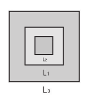
Figure 1: An open-boundary square lattice of linear size $L_{0}$ and its nested inner regions (linear sizes $L_{1}=L_{0}/2$ and $L_{2}=L_{0}/4$).

A) Single-Spin-Flip (SSF) algorithm

Because the NER method is based on the SSF dynamics, we study the NER of order parameters using a conventional SSF heat bath algorithm.

B) The CHB algorithm

We use the CHB algorithm in the equilibrium simulation because this algorithm reduces the number of MC sweeps in the relaxation. In the CHB algorithm, the spin configuration of a block of $L_{0}\times l_{y}$ spins is updated using the transfer matrix method, where the transfer direction is the $x$-direction ($L_{0}$) and $l_{y}$ is determined from the computational time costs. In this paper we apply the SM procedureSato with $l_{y}=6$.

We consider two quantities: the square of the chain magnetization (the magnetization along the $x$-axis) given by

$$M_{2}=\frac{1}{L}\sum_{y=1}^{L}(\frac{1}{L}\sum_{x=1}^{L}S_{x,y})^{2}.$$ (2)

$M_{2}$ is conventionally used to examine the phase transition of the model. We also consider the spin overlap function $q(\vec{k})$ of two spin configurations $\{S_{x,y}^{\alpha}\}$ and $\{S_{x,y}^{\beta}\}$ in independent MC runs:

$$q(\vec{k})=\frac{1}{L^{2}}\sum_{x=1}^{L}\sum_{y=1}^{L}S_{x,y}^{\alpha}S_{x,y}^{\beta}\exp(i\vec{k}\vec{r}_{x,y}).$$ (3)

From the $q(\vec{k})$, we investigate the nature of the phase transition.

III Equilibrium Simulation

We investigate the equilibrium properties of the ANNNI model by SM’s approach.Sato Especially, we are interested in whether the previous picture of the spin ordering emerges on larger lattices. Therefore, we extend the lattice size to the largest possible, up to $L_{0}\times L_{0}=512\times 512$ sites, with linear size eight times larger than that treated by SM.

The physical quantities were averaged from 16 independent simulation runs. The system is regarded as equilibrated when the difference in $\langle q(0)^{2}\rangle$ between two estimates obtained from two different MC sweeps (the one averaged over from $MCS_{equi}+1$ MC sweep to $MCS_{equi}+MCS_{mea}/2$ MC sweep and the other from $MCS_{equi}+MCS_{mea}/2+1$ MC sweep to $MCS_{equi}+MCS_{mea}$ MC sweep) becomes smaller than $1\%$, where $\langle...\rangle$ denotes the thermal average. About 80,000 MC sweeps were needed to equilibrate the system with $L_{0}=512$ at $T=1.15J$. The parameters used in the equilibrium simulation are listed in Table 1.

Table 1: Parameters used in the CHB algorithm of the MC simulation. $MCS_{equi}$ and $MCS_{mea}$ are the number of MC sweeps required for equilibration and measurement, respectively.

$L_{0}$	$MCS_{equi}$	$MCS_{mea}$
32	4,000	12,000
64	10,000	30,000
128	20,000	60,000
256	40,000	80,000
512	80,000	120,000

III.1 Chain magnetization

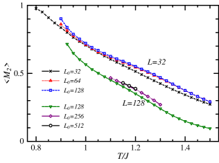
Figure 2: (color online) Lattice size $L_{0}$ dependences of $\langle M_{2}\rangle$ in the ANNNI model with $\kappa=0.6$ within regions $L=32$ and $L=128$. Error bars are smaller than the symbols.

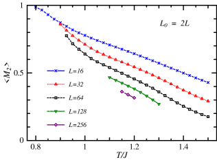
Figure 3: (color online) Temperature dependences of the square of the chain magnetization $\langle M_{2}\rangle$ in the ANNNI model with $\kappa=0.6$ within regions of different linear size $L$. Error bars are smaller than the symbols.

We first consider the square of the chain magnetization $\langle M_{2}\rangle$. To examine the surface effect, we plot $\langle M_{2}\rangle$ as a function of temperature within the inner regions $L=32$ and $L=128$ at different lattice sizes $L_{0}$. The results are shown in Fig. 2. We find that $\langle M_{2}\rangle$ increases with increasing $L_{0}$. Although $\langle M_{2}\rangle$ markedly differs between the whole lattice $L_{0}$ and the inner region $L_{1}$, it little varies between the inner regions $L_{1}$ and $L_{2}$. Therefore, we consider that the surface effect can be eliminated by conducting simulations over the inner region $L_{1}$. Figure 3 plots $\langle M_{2}\rangle$ in the inner region $L_{1}$ as a function of temperature. We investigate the phase transition in the model identically to SM.Sato If the IC phase occurs, the spin correlation function will decay according to a power law

$$\langle S_{\it{0,0}}S_{\it{x,y}}\rangle\sim r^{-\eta}\cos(qy)\hskip 14.22636pt{\rm for}\hskip 14.22636ptx,y\gg 1$$ (4)

where $r=\sqrt{x^{2}+y^{2}}$ and $\eta$ and $q$ are the decay exponent and the wave number, respectively. At the transition temperature $T_{c1}$ or below, the chain magnetization is described by

$$\langle M_{2}\rangle = \frac{1}{L}\sum_{y=1}^{L}\frac{1}{L}\sum_{x=1}^{L}\langle S_{1,y}S_{x,y}\rangle$$ (5)

$$\sim L^{-\eta}.$$ (6)

First, we examine this relationship. By tuning $\eta$, all of the $\langle M_{2}\rangle L^{\eta}-T/J$ curves can be made to cross at a single point. From this crossover point, $T_{c1}$ and $\eta$ are determined as approximately $1.16J$ and 0.25, respectively. The result is plotted in Fig. 4. Next we construct a finite-size scaling (FSS) plot, assuming the KT transitionKT

$$\langle M_{2}\rangle L^{\eta}=Y[L^{-1}\exp(b|\varepsilon|^{-0.5})],$$ (7)

where $\varepsilon=(T-T_{c1})/T_{c1}$ and $Y$ is some scaling function. Setting $T_{c1}$ and $\eta$ to approximately $1.16J$ and 0.25, respectively, and $b=2.2$, the curves neatly collapse at the higher temperature side $T>T_{c1}(=1.16J)$, as shown in Fig. 5. However, the FSS plots fail at the lower temperature side $T<T_{c1}$, implying that no long range order occurs at $T<T_{c1}$. We should note that the values estimated here are consistent with those estimated by SM on smaller lattices ($L_{0}\leq 64$), reported as $T_{c1}/J=1.16\pm 0.02,\eta=0.25\pm 0.02$ and $b\sim 2.2$.Sato

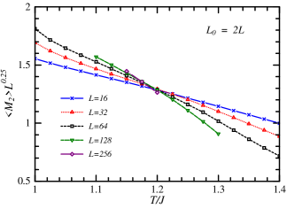
Figure 4: (color online) $\langle M_{2}\rangle L^{0.25}$ versus $T/J$.

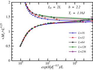
Figure 5: (color online) Finite-size scaling plots of the ANNNI model with $\kappa=0.6$, assuming the KT transition with the same parameters as SM.Sato

III.2 Spin overlap

We now consider the spin overlap function. The temperature dependence of $\langle q(0)^{2}\rangle$ over the whole lattice $L_{0}$ is plotted in Fig. 6. We find that $\langle q(0)^{2}\rangle$ is a decreasing function of temperature. Efficient methods have been developed for determining the transition temperature from the spin overlap function. Here, we apply these methods to investigate the phase transition. However, these methods examine the ratios of the moments of the spin overlap functions which yield scattered data. We then consider the spin overlap functions in the inner region with $L=L_{2}$.

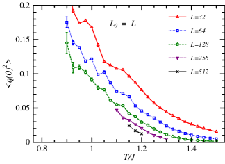
Figure 6: (color online) Temperature dependences of the spin overlap function $\langle q(0)^{2}\rangle$ in the ANNNI model with $\kappa=0.6$, computed over the whole lattice with $L=L_{0}$. Error bars that are not shown are smaller than the symbols.

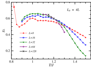
Figure 7: (color online) Temperature dependences of Binder ratio $g_{L}$ in the ANNNI model with $\kappa=0.6$ and different $L$. Error bars are smaller than the symbols.

First we consider the Binder ratio $g_{L}$Binder defined as

$$g_{L}=\frac{1}{2}\left(3-\frac{\langle q(0)^{4}\rangle}{\langle q(0)^{2}\rangle^{2}}\right).$$ (8)

The temperature dependences of $g_{L}$ for different $L$ are plotted in Fig. 7. At high temperatures, $g_{L}$ decreases with increasing $L$, indicating that no long range order establishes at these temperatures. As the temperature is decreased, $g_{L}$ for larger $L$ converge at $T\approx 1.18J$. Therefore, the Binder ratio $g_{L}$ supports that a phase transition occurs at $T=T_{c1}$. Below this temperature, the $L$ dependence of $g_{L}$ differs from that of usual systems exhibiting long-range order at low temperatures. That is, $g_{L}$ slightly increases with increasing $L$ and appears to converge to a single line. An analogous phenomenon occurs in the 2D XY model,2DXYBind indicating that the IC phase at $T\lesssim T_{c1}$ is indeed a KT type phase. Another remarkable feature is the behavior of $g_{L}$ as the temperature falls below $T_{c1}$; $g_{L}$ slightly increases, is maximized at $T\approx 1.05J$, and decreases below $T\approx 1.00J$. This behavior may imply that a different spin correlation develops below $T\approx 1.05J$. As is well-known, slightly above the lower transition temperature $T_{c2}$ the spin structure of the IC state is characterized by domain walls of three up-spin or down-spin chains that penetrate the $\langle 2\rangle$ phase.Selke2

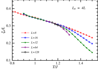
Figure 8: (color online) Correlation length ratio $\xi_{x}/L$ in the ANNNI model with $\kappa=0.6$ in the x direction. Error bars are smaller than the symbols.

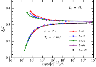
Figure 9: (color online) Finite-size-scaling plot of $\xi_{x}/L$ in the region $L=L_{2}$ assuming $T_{c1}=1.16J$.

III.3 Correlation length

Next we consider the spin correlation length $\xi_{\mu}$ ($\mu=x,y$) along the $\mu$-direction. This quantity is obtained from the spin overlap function as follows:

$$\xi_{\mu}=\frac{1}{2\sin(|\vec{k}_{\rm min}|/2)}\sqrt{\frac{\langle q(0)^{2}\rangle}{\langle|q({\vec{k}}_{\rm min})|^{2}\rangle}-1}$$ (9)

where ${\vec{k}}_{\rm min}=(\pi/L,0)$ and ${\vec{k}}_{\rm min}=(0,\pi/L)$ in the $x$- and $y$-direction, respectively. The ratio of the correlation length $\xi_{\mu}$ to the linear lattice size $L$, $\xi_{\mu}/L$, determines the transition temperature $T_{c}$.Cooper When $T>T_{c}$, $\xi_{\mu}$ is finite and $\xi_{\mu}/L\rightarrow 0$ as $L\rightarrow\infty$. On the other hand, at $T=T_{c}$, $\xi_{\mu}$ diverges in the thermodynamic limit and $\xi_{\mu}/L=C(\neq 0)$. Therefore, the $\xi_{\mu}/L$ for different $L$ cross at the phase transition temperature $T_{c}$. The correlation-length ratios $\xi_{x}/L$ for different $L$ are plotted as functions of $T$ in Fig. 8. At high temperatures, $\xi_{x}/L$ reduces at larger $L$, indicating that no long-range order establishes at these temperatures. As the temperature is decreased, the $\xi_{x}/L$ values increase for all $L$, and converge at approximately $T\approx 1.17J$. Below this temperature, they slowly increase at the same rate. This behavior is also observed in the 2D XY model.2DXYCorr To estimate the transition temperature $T_{c1}$, we construct an FSS plot of the $\xi_{x}/L$ values. The FSS plot collapses above $T_{c1}$, when $T_{c1}$ is assumed as $1.16J$(see Fig. 9).

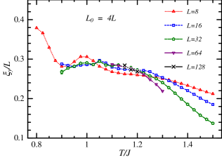
Figure 10: (color online) Correlation length ratio $\xi_{y}/L$ in the ANNNI model with $\kappa=0.6$ in the y direction. Error bars are smaller than the symbols.

Figure 10 plots the correlation-length ratio $\xi_{y}/L$ along the $y$-axis. Identically to their $\xi_{x}/L$ counterparts, the $\xi_{y}/L$ values for different $L$ converges at $T\approx 1.17J$. As the temperature decreases below $T_{c1}$, $\xi_{y}$ first slightly increases down to $T\approx 1.05J$, and slightly decreases thereafter, except for the data of $L=8$. This temperature dependence of $\xi_{y}$ at $T<1.05J$ differs from that of $\xi_{x}$. Specially, at $T<1.05J$, the spin correlations in the $x$-direction are enhanced as the temperature decreases, while those in the $y$-direction are suppressed.

III.4 Summary

We have investigated the phase transition in the 2D ANNNI model by conducting equilibrium MC simulations. We calculated the square of the chain magnetization in larger lattices of $L_{0}\times L_{0}$ sites ($L_{0}\leq 512$) and obtained $T_{c1}\approx 1.16J$, absolutely consistent with the results of the previous simulations on small lattices ($L_{0}\leq 64$). Thus, we conclude that the IC phase actually occurs in the ANNNI model.

We also calculated the Binder ratio $g_{L}$ of the spin overlap functions and the correlation-length ratios $\xi_{x}/L$ and $\xi_{y}/L$. At $T\lesssim T_{c1}$, these quantities behave similar to those in the 2D XY model. This suggests an analogy between the IC phase in the ANNNI model at $T\lesssim T_{c1}$ and the Kosteritz Thouless (KT) phase in the 2D XY model. Therefore, we can naturally refer to the phase transition at $T=T_{c1}$ as the KT phase transition.

IV NER Simulation

We now examine previous results of NER simulations. The NER method is based on the following hypothesis.ItoA ; ItoB In a system with a relevant order parameter $Q$ and a perfectly ordered initial state $Q(0)=1$ (or the PM phase $Q(0)=0$), MC simulations on a large lattice at temperature $T$ lead to three behaviors in the limit $t\rightarrow\infty$; (i) if $T>T_{c}$, $Q(t)$ decays exponentially, (ii) if $T<T_{c}$, $Q(t)$ converges toward some non-zero value, and (iii) if $T=T_{c}$, $Q(t)$ exhibits an algebraic decay (or an algebraic growth). In a critical state such as the KT phase, $Q(t)$ exhibits a behavior similar to that at $T=T_{c}$.

Shirahata and Nakamura(SN)Shirahata used the square of the chain magnetization $m_{l}(t)\ (\ \equiv\ M_{2}$ at $t$ MC sweep) as an order parameter of the IC phase. They performed MC simulations of the model with $\kappa=0.6$ starting with both the $\langle 2\rangle$ phase of $m_{l}(0)=1$ and the PM phase of $m_{l}(0)=0$. In the former case, they found that $m_{l}(t)$ decays exponentially at $T>0.98J$; in the latter, it tends to saturate at $T>0.92J$. From these results they predicted that $T_{c1}<0.92J$. Applying a finite time scaling analysis they refined this result to $T_{c1}\sim 0.89J$, close to the $\langle 2\rangle$ phase transition temperature $T_{c2}\sim 0.89J$ estimated from finite time scaling analysis of the $\langle 2\rangle$ phase magnetization. Similarly, Chandra and Dasgupta(CD)Chandra found that the order parameter $m_{l}(t)$ algebraically decays at $T\approx 1.00J$. Their transition temperature $T_{c1}\approx 1.00J$ and $T_{c2}\approx 1.00J$ (the latter estimated from relaxation of the energy) are also extremely close. Therefore, the NER method predicts the absence of the IC phase.

Besides the considerably different values of $T_{c1}$ (approximately $T_{c2}$) between estimated by SN and CD, the NER method raises some pertinent issues: (i) The exponential decay of $m_{l}(t)$ suggests that only the $\langle 2\rangle$ phase is unstable; it does not reveal the instability of the IC phase. In fact, $m_{l}(t)$ rebounds as the simulation proceeds.Chandra Rather, the stability of the IC phase should be examined by relaxation from an equilibrium state in the IC phase at $T_{c2}<T<T_{c1}$ (if present); (ii) The initial growth results of $m_{l}(t)$ reported by SNShirahata are not convincing. As seen in Fig. 3, the equilibrium value of $m_{l}(t)$, $\langle M_{2}\rangle$, is higher for the small $L$ than for the large $L$. However, $m_{l}(t)$ depicted in Fig. 6 of SNShirahata is independent of the linear lattice size $L_{x}$ at $t<10^{4}$ and increases with $L_{x}$ at $t>10^{4}$. We consider that the growth of $m_{l}(t)$ from the PM phase should be reexamined.

Here, we consider two phenomena: (i) The ordering process of the system initialized to non-equilibrium states and (ii) The dynamics of the system in the equilibrium state. Equivalently, we investigate the autocorrelation function in the equilibrium state. Since a huge number of MC sweeps are required to reach equilibrium, we implement the system on small lattices ($L_{0}\leq 512$).

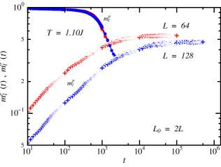
Figure 11: (color online) Relaxations of $m_{l}^{a}(t)$ and $m_{l}^{p}(t)$ in the ANNNI model with $\kappa=0.6$ at $T=1.10J$, slightly lower than $T_{c1}=1.16J$ estimated in the equilibrium simulation.

IV.1 Relaxations from the $\langle 2\rangle$ phase and the PM phase

Starting with the $\langle 2\rangle$ phase and the PM phase, we investigate the relaxation of the system. The system is implemented on the lattice described in Sec. II with $N(=64\sim 256)$ sets of spin configurations. At each MC sweep $t$, the square of the chain magnetization $m_{l}^{\mu}(t)$ is computed:

$$m_{l}^{\mu}(t)=\overline{M_{2}(t)},$$ (10)

where $M_{2}(t)$ is defined by eq.(2) at MC sweep $t$ and $\overline{\cdots}$ is the configuration average. The PM phase and the $\langle 2\rangle$ phase initial states are distinguished by setting the superscript $\mu=p$ and $a$, respectively.

Figure 11 plots the time courses of $m_{l}^{p}(t)$ and $m_{l}^{a}(t)$ calculated by the model on lattices with $L_{0}=128$ and $L_{0}=256$ at $T=1.10J$. Initially, $m_{l}^{p}(t)$ grows while $m_{l}^{a}(t)$ decays. At later times, the two quantities exhibit quite different temporal behaviors. While $m_{l}^{p}(t)$ monotonically increases and eventually saturates, $m_{l}^{a}(t)$ rapidly decreases, intercepts $m_{l}^{p}(t)$, and then increases along it. This rebound of $m_{l}^{a}(t)$ has been previously reported by CD.Chandra Importantly, $m_{l}^{a}(t)$ saturates at a much higher value than its minimum, and the minimum and saturation levels widen with increasing $L$. That is, the $\langle 2\rangle$ phase breaks once and a spin correlation of the IC state develops. The existence of the IC phase is examined by the equilibrium simulation performed in Sec. III. Another notable behavior is the large $L$-dependence of $m_{l}^{p}(t)$, which strongly contrasts with the SN results.Shirahata This behavior is reasonable because the square of the chain magnetization $m_{l}^{\mu}$ is related to the chain susceptibility $\chi_{l}^{\mu}(t)$ by

$$m_{l}^{\mu}(t) = \frac{1}{L}\chi_{l}^{\mu}(t).$$ (11)

If the spin correlations are not extensively developed, the chain susceptibility should become independent of $L$ at large $L$ and thereby reveal the NER properties of the system. The time courses of the susceptibility $\chi_{l}^{p}(t)(\equiv m_{l}^{p}(t)L)$ for different $L$ are plotted at $T=1.10J$ and $T=1.25J$ in Figs.12 (a) and (b), respectively. Note that as $L$ increases, $\chi_{l}^{p}(t)$ converges at small $t$. Following SN, we take $\chi_{l}^{p}(t)$ in the thermodynamic limit when the $\chi_{l}^{p}(t)$’s of two lattice sizes $L$ collapse onto the same line. The NER properties can be inferred from these $\chi_{l}^{p}(t)$, or we can examine the critical growth of $\chi_{l}^{p}(t)$ in the linear region of a $log(\chi_{l}^{p}(t))$ versus $log(t)$ plot. This range is called the algebraic range and its upper bound is denoted by $\tau$. At $T=1.10J$, $\tau$ appears to increase with $L$ implying that $\tau\rightarrow\infty$ as $L\rightarrow\infty$. On the other hand, $\chi_{l}^{p}(t)$ at $T=1.25J$ starts saturating for smaller $t$. The different behaviors of $\tau$ between these two temperatures become more conspicuous in the spin overlap function $q(t)$ (see Appendix). However, this speculation requires confirmation in complementary investigations.

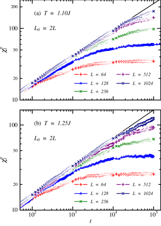
Figure 12: (color online) Growth of $\chi_{l}^{p}(t)(\equiv m_{l}^{p}(t)L)$ for different $L$ at (upper panel) $T=1.10J$ (slightly lower than $T_{c1}$) and (lower panel) $T=1.25J$ (slightly higher than $T_{c1}$). The straight line in each plot is least-squares fitted to the data of $L=1024$ from $50\leq t\leq 5,000$.

IV.2 Autocorrelation function in the IC phase

As shown above, the rapid decay of $m_{l}^{a}(t)$ nor $q^{a}(t)$ does not reveal the instability of the IC phase. Here we examine the system dynamics in the IC phase by the following procedure. First we construct $N(=64-128)$ equilibrium spin configurations $\{S_{xy}^{(n)}(0)\}$ $(n=1-N)$ at a specified temperature $T$, varying the initial spin configurations. Starting from these equilibrium spin configurations, we conduct MC simulations using the SSF algorithm and obtain the spin configurations $\{S_{xy}^{(n)}(t)\}$ at the $t$-th MC sweep. The dynamics of the evolving spin configurations are obtained from the autocorrelation function $C(T,t)$ defined as

$$C(T,t)=\frac{1}{N}\sum_{n}\frac{1}{L^{2}}\sum_{x}\sum_{y}S_{x,y}^{(n)}(0)S_{x,y}^{(n)}(t).$$ (12)

At $t=0$, $C(T,0)=1$. As $t\rightarrow\infty$, $C(T,t)\rightarrow\langle S\rangle^{2}$, where $\langle S\rangle$ is the average of $S_{x,y}$ in the equilibrium state. Then, $C(T,t)$ converges to some positive value at $T<T_{c}$, but exponentially decays at $T>T_{c}$. At $T=T_{c}$ or in a critical state, $C(T,t)$ undergoes algebraic decay. In other words, $C(T,t)$ plays the same role as the order parameter $Q(t)$ in the NER simulation. We now calculate $C(T,t)$ at two $T$ for different $L$.

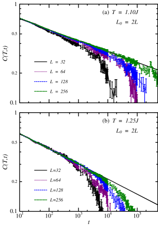
Figure 13: (color online) Autocorrelation function $C(T,t)$ in the ANNNI model with $\kappa=0.6$ for different $L$ in the equilibrium state at (upper panel) $T=1.10J$ and (lower panel) $T=1.25J$. The straight line is least-squares fitted to the data of $L=256$ from $50\leq t\leq 5,000$.

The time courses of $C(T,t)$ at $T=1.10J$ and $T=1.25J$ are plotted in Figs. 13 (a) and (b), respectively. The $L$ dependence of $C(T,t)$ differs between these two temperatures. At $T=1.10J$, the algebraic range extends as $L$ increases, while for $T=1.25J$ it apparently terminates at $t\approx 5000$. We make a least-squares fitting to the function $C(T,t)=At^{-\lambda}$ for the data of $L=256$ from $50\leq t\leq 5,000$ and the upper bound of the algebraic range $\tau$ is estimated.tau Figure 14 plots $\tau$ as a function of $L$ at both temperatures. At $T=1.10J$, $\tau$ appears to extend as $\tau\propto L^{z}$ with $z\approx 2$, while at $T=1.25J$ it seems to saturate. This suggests that $1.10J<T_{c1}<1.25J$.

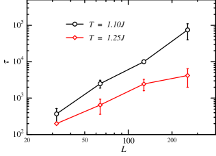
Figure 14: (color online) Algebraic time ranges $\tau$ of the correlation function $C(T,t)$ as functions of linear lattice size $L=L_{0}/2$ at $T=1.10J$(black) and $T=1.25J$(red).

IV.3 Summary

Examining the results of recent NER studies on the ANNNI model, we find that claims of the absence of the IC phase are not convincing.

We have reexamined the growth of the IC phase from the PM phase by observing the behaviors of the chain magnetization $m_{l}$ and the spin overlap $q$. Both quantities of $m_{l}^{p}(t)L$ and $q^{p}(t)L$ appear to algebraically increase with $t$ at $T=1.10J$. We also investigated the autocorrelation function $C(T,t)$ in the equilibrium state and found that it algebraically and exponentially decays over time at $T=1.10J$ and $T=1.25J$, respectively. In stark contrast to the previous reports, we conclude that the NER method predicts the occurrence of the IC phase below $T_{c1}$ with $1.10J<T_{c1}<1.25J$.

V Conclusion

The spin structure of the 2D ANNNI model is a renewed problem because the spin ordering picture in recent large scale Monte Carlo (MC) simulations depends on the simulation method. Specially, the equilibrium simulation predicts a floating incommensulate (IC) phase of Kosterlitz-Thouless (KT) type, whereas the non-equilibrium relaxation (NER) simulation predicts the absence of this phase. In this paper, we examined recently published results of equilibrium and NER simulations and investigated the spin ordering of the model with frustration ratio $\kappa=0.6$ in both simulation methods. Both methods yielded a KT type phase transition between the paramagnetic phase and the IC phase at $T_{c1}\approx 1.16J$.

The present paper focused on the upper phase transition at $T_{c1}$. The other phase transition at $T_{c2}$, between the IC phase and the $\langle 2\rangle$ phase, will be investigated in a separate paper.

Appendix A

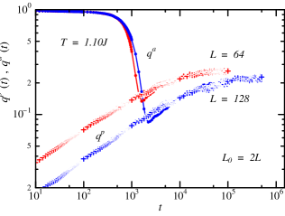
Figure 15: (color online) Relaxations of $q^{a}(t)$ and $q^{p}(t)$ in the ANNNI model with $\kappa=0.6$ at $T=1.1J$ (slightly lower than $T_{c1}$).

The spin overlap $q^{\mu}(t)$ is calculated as

$$q^{\mu}(t)=\frac{2}{N(N-1)}\sum_{m\neq n}|\frac{1}{L^{2}}\sum_{x=1}^{L}\sum_{y=1}^{L}S_{x,y}^{(m)}(t)S_{x,y}^{(n)}(t)|,\hskip 14.22636pt$$ (13)

where $N(=64-256)$ is the number of spin configuration sets {$S_{x,y}^{(n)}(t)\}$ ($n,m=1-N$) and $t$ is the MC sweep. Figure 15 plots the time courses of $q^{p}(t)$ and $q^{a}(t)$ with $L_{0}=128$ and $L_{0}=256$ at $T=1.10J$. The temporal behaviors are quite similar to those of $m_{l}^{p}(t)$ and $m_{l}^{a}(t)$ in Fig. 11.

Figure 16 plots the time courses of $q^{p}(t)L$ for different $L$ at $T=1.10J$(upper panel) and $T=1.25J$(lower panel). At $T=1.10J$ and $L=1024$, $q^{p}(t)L$ algebraically grows up to $t=5\times 10^{4}$, whereas at $T=1.25J$ it starts to saturating at $t>5\times 10^{3}$.

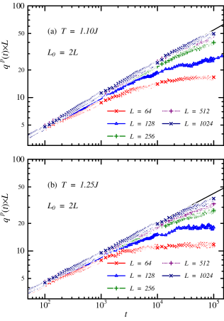
Figure 16: (color online) Growth of $q^{p}(t)$ in the ANNNI model with $\kappa=0.6$ at $T=1.10J$(upper) and $T=1.25J$(lower) for different $L$. The straight line in each plot is least-squared fitted to the data of $L=1024$ from $50<t<5,000$.

References

References

- (1) For example see, e.g., W. Selke, in PHASE TRANSITIONS AND CRITICAL PHENOMENA, ed. C. Domb and J. L. Lebowitz (Academic Press, 1992), Vol. 15, p. 1; and references therein.
- (2) W. Selke and M.E. Fisher, Z. Physik B 40, 71 (1980).
- (3) W. Selke, K. Binder, and W. Kinzel, Surf. Sci. 125, 74 (1983).
- (4) J. M. Kosterlitz and D. J. Thouless, J. Phys. C6, 1181 (1973).
- (5) J. Villain and P. Bak, J. Phys.(Paris) 42, 657 (1981).
- (6) M. D. Grynberg and H. Ceva, Phys. Rev. B 36, 7091 (1987).
- (7) M. A. S. Saqi and D. S. McKenzie, J. Phys. A: Math. Gen. 20 471 (1987).
- (8) Y. Murai, K. Tanaka and T. Morita, Physica A 217, 214 (1995).
- (9) A. Sato and F. Matsubara, Phys. Rev. B 60, 10316 (1999).
- (10) O. Koseki and F. Matsubara, J. Phys. Soc. Jpn. 66, 322 (1997).
- (11) F. Matsubara, A. Sato, O. Koseki, and T. Shirakura, Phys. Rev. Lett. 78, 3237 (1997).
- (12) T. Shirahata and T. Nakamura, Phys. Rev. B 65, 024402 (2001).
- (13) N. Ito, Physica A 192, 604 (1993).
- (14) N. Ito and Y. Ozeki, Int. J. Mod. Phys. C 10, 1495 (1999).
- (15) E. Rastelli, S. Regina and A. Tassi, Phys. Rev. B 81, 094425 (2010).
- (16) A. K. Chandra and S. Dasgupta, J. Phys. A: Math. Theor. 40 6251 (2007).
- (17) K. Binder, Z. Phys. B: Condens. Matter 43, 119 (1981).
- (18) F. Cooper, B. Freedman, and D. Preston, Nucl. Phys. B 210, 210 (1989).
- (19) E. Iñiguez, E. Marinari, G. Parisi, and J. J. Ruiz-Lorenzo, J. Phys. A 30, 7337 (1997).
- (20) H. G. Ballesteros, A. Cruz, L. A. Fernández, et al., Phys. Rev. B 62, 14237 (2000).
- (21) We roughly estimate as follows. We first obtain the fitting function of using the least-squares method for the data of from , and the relative difference is calculated. When is increased from a small , increases with fluctuation. The algebraic ranges and are defined such that at which firstly becomes and , respectively. We estimate .