Thermodynamics of inequalities:
from precariousness to economic stratification

Abstract

Growing economic inequalities are observed in several countries throughout the world. Following Pareto, the power-law structure of these inequalities has been the subject of much theoretical and empirical work. But their nonequilibrium dynamics, e.g. after a policy change, remains incompletely understood. Here we introduce a thermodynamical theory of inequalities based on the analogy between economic stratification and statistical entropy. Within this framework we identify the combination of upward mobility with precariousness as a fundamental driver of inequality. We formalize this statement by a “second-law” inequality displaying upward mobility and precariousness as thermodynamic conjugate variables. We estimate the time scale for the “relaxation” of the wealth distribution after a sudden change of the after-tax return on capital. Our method can be generalized to gain insight into the dynamics of inequalities in any Markovian model of socioeconomic interactions.

1 Introduction

All known human societies have displayed some level of economic inequality [2]. Yet this global imbalance is reaching alarming levels in the contemporary world: as of 2013, the 400 richest Americans have more wealth than the bottom half of all Americans combined. Indeed recent comprehensive research [3] has showed that, while they have not reached the highs of the pre-1929 period, wealth inequalities in developed countries have steadily increased in the past decades. Understanding the origins and implications of these inequalities is an outstanding problem for economics, but also for society as a whole.

On the theory side, a well-established approach to this problem—pursued independently by economists [4], mathematicians [5, 6], sociologists [7] and physicists [8, 9, 10]—consists in studying the equilibrium wealth distribution in stochastic models of individual (or household) income. Under general assumptions, one shows that additive income lead to exponential distributions, while multiplicative capital returns yield Pareto-like power law distributions [11, 12, 13, 14, 15]. These results are consistent with empirical data, both contemporary [16] and historical [17], which reveal a two-class structure with an exponential range at low wealth (where investment is negligible) and a power-law tail at high capital (where income is dominated by investment returns). Econophysicists [10] have pointed the striking similarity between this pattern and the Boltzmann-Gibbs distribution of statistical mechanics. Indeed both have the same “entropic” structure: there are many more ways to distribute a conserved quantity (be it wealth or energy) unequally than equally.

One much discussed consequence of such marked economic inequalities is the emergence of a super-elite class, the so-called “top $1\%$” [18], with disproportionate social, economical and political influence. But they also have more global effects, one of which is increased stratification [19]—the growth of the number of economically distinct “classes” in society. Indeed, as we will see below, “maximum entropy” wealth distributions are precisely those with the greatest stratification under global constraints on the mean wealth. This intriguing analogy between entropy and stratification points to a connection between the dynamics of inequalities and dissipation in thermal systems, extending beyond the limits of equilibrium statistical mechanics (to which it has been restricted so far).

In this paper we introduce a general framework, inspired from stochastic thermodynamics [20], to account for the dynamical origin of social inequalities. At its foundation is a general property of Markov processes known as the fluctuation theorem (Appendix A). As we shall see, the great strength of this theorem lies in its explanatory power: given an entropy-increasing stochastic process, the fluctuation theorem elucidates the mechanism driving entropy production. In the context of social inequalities, where entropy quantifies inequality, we find that, over and above the multiplicative effect of capital return, precarious social mobility acts as a universal inequality-generating mechanism.

2 Results

2.1 Stratification

We begin by formalizing our notion of stratification. Let $w\in[w_{min},w_{max}]$ denote the wealth of an individual (or household) in the economy. The wealth distribution $p_{t}(w)$ is the probability density function (PDF) at time $t$ for the wealth variable $w$, i.e. $p_{t}(w)dw$ gives the probability of finding an agent with wealth at time $t$ between $w$ and $w+dw$, or the fraction of population whose wealth is between $w$ and $w+dw$ at that time.

Given $\delta w$ a reference wealth unit, we call economic stratum a segment of the population with wealth in the range $[w_{i},w_{i+1}]$ where $w_{i}=w_{min}+b^{i}\delta w$ for some conventional number $b>1$. For instance, we could take $\delta w=\$1$ and $b=10^{3}$, in which case the words “millionaire” and “billionaire” would correspond to the adjacent strata $i=3$ and $i=4$.

Next we define the stratification $S_{t}$ of the population at time $t$ by

$$S_{t}\equiv-\int_{w_{min}}^{w_{min}}p_{t}(w)\log\,p_{t}(w)\,dw-\log\delta w,$$ (1)

where $\log$ is the base $b$ logarithm. (Mathematically, $S_{t}$ is the “differential entropy” of the wealth distribution $p_{t}(w)$.) Stratification is maximized by the uniform distribution on the interval $[w_{min},w_{max}]$, in which case it simply measures the number of strata in the population. This feature is to be contrasted with the Gini index commonly used in the social sciences to measure economic inequalities:

$$G_{t}\equiv 1-\frac{1}{\langle w\rangle_{t}}\int_{w_{min}}^{w_{min}}\left[1-\int_{w_{min}}^{w}p_{t}(w^{\prime})\,dw^{\prime}\right]^{2}\,dw$$ (2)

where $\langle w\rangle_{t}$ is the mean of the distribution $p_{t}(w)$. Indeed, $G_{t}$ is maximized not by uniform wealth distributions, but by the (highly unrealistic) “state of extreme inequality” in which one agent has all wealth, and all $N-1$ other agents have nothing: $p(w)=(1-N^{-1})\delta(w-w_{min})+N^{-1}\delta(w-w_{max})$. The fact that the Gini index is maximized by such a singular distribution makes it rather unnatural in the context of large populations with smooth, unimodal distributions. This being said, in many cases of interest the Gini index turns out to be an increasing function of stratification, as illustrated in Fig. 1.

Figure 1: Comparison of the Gini and stratification indices for three familiar distributions: Pareto distributions with threshold $w_{min}$ and tail index $\alpha$, normal distributions with mean $m$ and standard deviation $s$, and lognormal distributions with local parameter $\mu$ and scale parameter $\sigma$. Here we fix $w_{min}=m=\mu=1$ and $\delta w=1$ and vary $\alpha$, $s$ and $\sigma$ respectively.

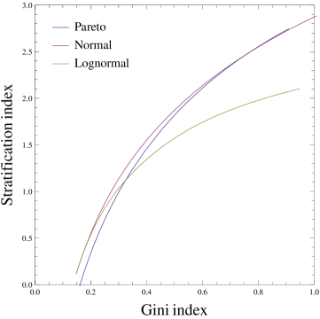
It is remarkable that both the Boltzmann (exponential) and Pareto (power-law) distributions, which have been argued to describe the empirical wealth distributions in the lower and higher quantiles respectively, arise as maximum stratification distributions. Indeed, the former corresponds to the maximum of $S$ under the constraint $\langle w\rangle=1/\beta$, while the latter corresponds to the maximum of $S$ under the constraint $\langle\log(w/w_{min})\rangle=1/\alpha$. (One can check that $S$ is a monotonically decreasing function of $\beta$ and $\alpha$ respectively.) In other words, the lower (resp. higher) quantiles of society appear to be maximally stratified given a fixed mean additive (resp. multiplicative) wealth: using the language of statistical mechanics, we could say that the “poor” and “rich” segments of society are close to statistical equilibrium given their constraints. This observation begs a question: how is this social equilibrium reached?

2.2 A toy model

Figure 2: Numerical verification of the fluctuation theorem in a toy society with $K=10$ classes, for two different initial distributions $p_{0}(k)$. In the top row, almost all individuals start in the lowest class ($p_{0}(k)=91\%$ if $k=1$ and $p_{0}(k)=1\%$ else). In the bottom row, the initial population is uniformly distribution over the $K$ classes ($p_{0}(k)=1/K$). Here $\pi_{+}=30\%$, $\pi_{-}=50\%$, $b=2$, and the statistics were computed over $10^{4}$ realizations of the process. The histograms show the distribution of class variations $\Delta k=k_{T}-k_{0}$ in the numerical experiment.

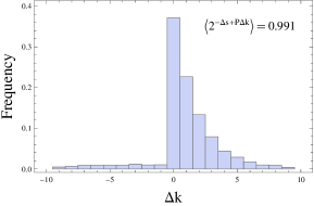
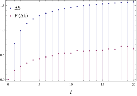
To begin investigating this question, consider the following toy model of society. Assume a finite set of “classes” $k=1,2,\dots,K$, and suppose that at each time step $t$ there is a probability $\pi_{+}$ (resp. $\pi_{-}$) for each individual to move up (resp. down) one class. (Here a “class” could be an economic stratum in the sense above, or indeed any other form of social ladder: political power, fame, etc.) We call the log-ratio $P=\log(\pi_{-}/\pi_{+})$, which measures of the tendency to go down the social ladder, the precariousness parameter.

The history of an individual in this toy society consists of a Markov chain of classes $k_{0}$, $k_{1}$, $k_{2}$… At each time $t$, the probability to find an individual in class $k$ is the class distribution $p_{t}(k)$. To this distribution we associate the surprisal $s_{t}(k)\equiv-\log p_{t}(k)$; its expectation value is the stratification $S_{t}\equiv-\sum_{k}p_{t}(k)\log p_{t}(k)$.

Now, the fluctuation theorem for Markov chains (Appendix A.2) states that, after any given number of time steps $T$, the difference $\Delta s-P\Delta k\equiv s_{T}(k_{T})-s_{0}(k_{0})-P(k_{T}-k_{0})$ is a random variable with the following properties:

1. The probability distribution of $\Delta s-P\Delta k$ is such that the expected value

   $$\langle b^{-\Delta s+P\Delta k}\rangle=1.$$ (3)

   This identity implies that $\Delta s-P\Delta k$ is exponentially unlikely to be negative, in the sense that for any positive number $r$,

   $$\textrm{Prob}[\Delta s-P\Delta k\leq-r]\leq b^{-r}.$$ (4)

2. As a consequence of this identity, the variation of the stratification $\Delta S=S_{T}-S_{0}=\langle\Delta s\rangle$ during the process is constrained by the second law inequality

   $$\Delta S\geq P\langle\Delta k\rangle.$$ (5)

   In other words, in this toy society,

   $$(\textrm{stratification increase})\geq(\textrm{precariousness})\times(\textrm{upward mobility}).$$ (6)

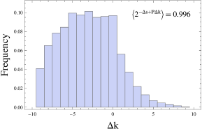
Suppose for instance that all individuals started off in the lowest class $k=1$, so that $S_{0}=0$, and that $\pi_{-}<\pi_{+}$, so that downward social evolution is more likely than upward social evolution. Then the second law indicates that, as the mean class level $\langle k\rangle$ grows, so does the stratification, at a rate greater than $P$ per class level. We illustrate the results (4) and (5) in Fig. 2 for two different initial class distributions $p_{0}(k)$.

2.3 Stochastic wealth model: “second law” inequality

Armed with this basic intuition, let us now depart from the simplistic notion of “classes” and get back to continuous wealth distributions. Denote $w_{t}$ be the detrended wealth of a household at time $t$. We assume a stochastic dynamics of the form

$$dw_{t}=ldt+w_{t}\cdot(\rho dt+\sigma dB_{t}).$$ (7)

The first term describe “additive” income (labor), while the second term represents “multiplicative” income (capital returns). In the notations of [23], the mean return rate $\rho$ is given by $\rho=\bar{r}-g-c$, where $\bar{r}$, $g$ and $c$ represent the after-tax return, growth and consumption rates respectively. We assume that the return shocks $dB_{t}$ form a standard Brownian motion (Wiener process) and we use the Ito convention for stochastic differentials [24]. A dictionary between the terms used in this section and more standard physics terminology is provided in Appendix D.

Stochastic wealth models such as (7) have been considered by many authors, see [25] and references therein. In particular, stochastic equations of the form (7) arise in the “random-agent” approximation of certain agent-based models [26]. In this setting one shows [9] that the stationary distribution—an inverse Gamma distribution—has a Pareto tail with exponent $\alpha=1-2\rho/\sigma^{2}$, which decreases when $\bar{r}-g$ increases [23]. (When $\rho\geq\sigma^{2}/2$, the model does not have an equilibrium distribution.)

Here we are interested in the non-equilibrium dynamics of stratification. As in the discrete case, this problem can be investigated using the fluctuation theorem for diffusion processes [27, 28, 29], see Appendix A.3. This gives the exact analogue of relations (3) and (4), with the entropy “source” term $P\Delta k$ replaced by the Stratonovich stochastic integral

$$\int_{0}^{T}P(w_{t})\circ dw_{t}=\int_{0}^{T}P(w_{t})\cdot dw_{t}-\frac{1}{2}\int_{0}^{T}P^{\prime}(w_{t})dt.$$ (8)

Here the notations $\cdot\,dw_{t}$ and $\circ\,dw_{t}$ refer to the Ito and Stratonovich conventions for stochastic integrals (see e.g. [24]), and we defined the precariousness function (plotted in Fig. 3)

$$P(w)=\frac{2}{\ln b}\left(\frac{\sigma^{2}-\rho}{\sigma^{2}w}-\frac{l}{\sigma^{2}w^{2}}\right).$$ (9)

In particular, the second law inequality now reads

$$\frac{dS_{t}}{dt}\geq\int P(w)\,j_{t}(w)\,dw$$ (10)

where $j_{t}(w)$ is the “social mobility flux”, i.e. the expected enrichment rate of a household with wealth $w$. The social mobility flux is given by

$$j_{t}(w)=(l+\rho w)p_{t}(w)-\frac{\sigma^{2}}{2}\partial_{w}(w^{2}p_{t}(w))$$ (11)

and satisfies the continuity (Fokker-Planck, forward Kolmogorov) equation

$$\partial_{t}p_{t}(w)+\partial_{w}j_{t}(w)=0.$$ (12)

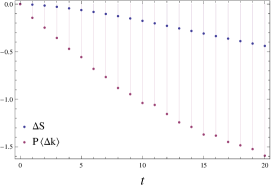
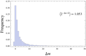
The inequality (10) becomes an identity in the limit of small flux $j_{t}(w)$, i.e. close to statistical equilibrium. Fig. 4 shows a numerical verification of the fluctuation theorem in this case.

Figure 3: The precariousness $P(w)$ (left) and potential $V(w)$ (right) functions for various values of $\rho=\bar{r}-g-c$ at fixed volatility $\sigma$. Here the wealth $w$ is expressed in units of labor income per investment period and we take $\sigma^{2}=10\%$ per period. The notion of precariousness remains meaningful even in the absence of an equilibrium distribution ($\rho\geq\sigma^{2}/2$, dashed lines).

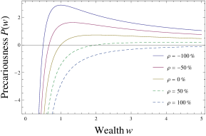
This result sheds an interesting new light on the relationship between economic conditions and social inequalities. First, when $\rho\leq\sigma^{2}$, the precariousness function $P(w)$ changes sign at the threshold wealth

$$w_{*}=\frac{l}{\sigma^{2}-\rho}.$$ (13)

This threshold has a simple interpretation: enrichment $j_{t}(w)>0$ at $w<w_{*}$ decreases the stratification, while enrichment $j_{t}(w)>0$ at $w>w_{*}$ increases it. This result formalizes the intuitive notion that enriching the poor reduces inequalities, while enriching the rich increase inequalities.

Second, all other things being equal, this critical wealth $w_{*}$ is an increasing function of $\bar{r}-g$. This means that a larger capital return rate allows growth to have an inequality-alleviating effect on more quantiles of the population. (This is of course assuming that these quantiles actually participate in multiplicative investments—which of course is not true of the poorer strata of society). Note also that $w_{*}$, like the Pareto exponent $\alpha$, is a decreasing function of the volatility $\sigma$. Thus, like in our toy model, the growth of inequalities can be interpreted as a consequence of risk [14].

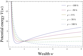
Third, the precariousness function $P(w)$, which we saw controls the dynamics of stratification out of wealth equilibrium, turns out to be directly related to the equilibrium wealth distribution $p_{\textrm{eq}}(w)$. Indeed, the latter, obtained by setting $j_{\textrm{eq}}=0$ in equation (11), is simply given by

$$p_{\textrm{eq}}(w)\propto b^{-V(w)}$$ (14)

where

$$V(w)\equiv\int^{w}P(w^{\prime})dw^{\prime}.$$ (15)

The potential function $V(w)$ is plotted in Fig. 3. Thus, from this perspective, the relevant “conserved quantity” in the economy is $V(w)$, and not wealth $w$ itself (as proposed in [10] but criticized in [30]). Identifying such a conserved quantity (in physics parlance, a “potential” function) provides useful intuition for the stochastic dynamics (7): roughly speaking, each household tries to reach the minimum of $V(w)$ (the zero-precariousness threshold value $w=w_{*}$), but is constantly driven away from that value by stratification-maximizing “fluctuations”. In this sense, the potential $V(w)$ can be thought of as the mathematical expression of a Smithian “invisible hand” driving macroeconomic evolution [31].

Figure 4: Left: five sample paths $w_{t}$ illustrating the main qualitative feature of the stochastic wealth model (7): most paths converge to $w\simeq w_{*}$ and remain there forever, but some paths make wild excursions at large wealth (the “top $1\%$” tail of the Pareto distribution). Right: histogram of net gains $\Delta w$ after $T=100$ and verification of the integral fluctuation relation over $10^{4}$ paths ($\Sigma$ denotes the stochastic integral (8)). In both plots the initial wealth is normally distributed about $w=1$ (with standard deviation $.1$) and $\rho=-10\%$, $l=1$, $\sigma^{2}=100\%$ per period.

2.4 Stochastic wealth model: relaxation time

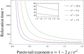
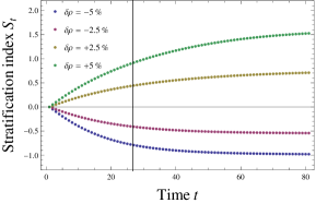
An important question which is readily addressed in this nonequilibrium framework is that of the relaxation time of the economy. Suppose that, starting from the equilibrium wealth distribution for the parameters $(l,\rho,\sigma$) and Pareto tail exponent $\alpha=1-2\rho/\sigma^{2}$, the detrended effective return rate $\rho$ suddenly changes to the value $\rho^{\prime}=\rho+\delta\rho$ (e.g. because $\bar{r}-g$ changes according to new fiscal policies): how long will it take for the economy to reach the new statistical equilibrium with Pareto tail exponent $\alpha^{\prime}=1-2\rho^{\prime}/\sigma^{2}$? A straightfoward computation using the formalism above allows us to estimate the relaxation time (to first order in $\delta\rho$) as (Appendix C)

$$\tau\simeq\frac{2\psi_{1}(\alpha)(1+\alpha)-2}{\sigma^{2}},$$ (16)

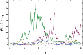
where $\psi_{1}$ is the trigamma function. Note that, at this order, the relaxation time $\tau$ is independent of $\delta\rho$: larger changes $\delta\rho$ lead to larger changes of the stratification $\delta S$, but these changes always occur on the same time scale $\tau$. The latter is also independent of $l$, implying that increasing labor income does not affect the dynamics of inequalities. Finally, $\tau$ increases with $\bar{r}-g$ and is very sensitive to the volatility $\sigma$, see Fig. 5.

Figure 5: Left: the relaxation time (16) as a function of $\alpha=1-2\rho/\sigma^{2}$. Notice the strong dependence on the volatility $\sigma$ (inset: zoom on the $1.5\leq\alpha\leq 2$ region). Right: Stratification as a function of time, starting from the equilibrium distribution for six different values of $\delta\rho$ (the vertical line represents $t=\tau$). Here $\rho=-2.5\%$, $\sigma^{2}=10\%$ and $l=1$ per period.

3 Conclusion

Using the fluctuation theorem for Markov processes as a guide, we have identified precarious mobility as a key driver of inequalities away from equilibrium. We have illustrated this idea in simple stochastic wealth models, where we obtained lower bounds on the growth of stratification over time as well as estimates of the corresponding time scales. But the scope of our approach is broader, and can be generalized to other stochastic models of socioeconomic dynamics: in Appendix B we apply the fluctuation theorem to a model of (biased) trade and find an upper bound on the so-called Theil inequality index.

Our results are complementary to earlier findings which showed that high interest rates (for given growth rate) generate fat-tailed, Pareto-like equilibrium distributions [4, 5, 6, 7, 9, 10, 11, 12, 13, 14]. In particular, they throw light on the question: how will the economic system “respond” to a perturbation? We saw for instance that there exists a threshold wealth $w_{*}$ beyond which enrichment generates more inequalities. Such knowledge provides a clear guideline regarding the quantiles which should be targeted by redistribution policies ($w<w_{*}$), and the ones which should not ($w>w_{*})$. In the current crisis times, we believe that developing further a “response theory” of the economic system is a pressing challenge for political economy.

Appendix A The fluctuation theorem

A.1 General idea

The (integral) fluctuation theorem is a general property of Markov stochastic processes. It states that there exists a function $\Sigma$ of stochastic paths such that [29]

$$\langle b^{-\Delta s-\Sigma}\rangle=1,$$ (17)

where $\Delta s=\log[p_{0}(X_{0})/p_{T}(X_{T})]$ is difference between the initial and final surprisal. Here $X_{t}$ is the state of the system at time $t$ and $p_{t}(X)$ is the corresponding probability distribution. The identity (17) implies that paths such that $\Delta s-\Sigma<0$ are exponentially unlikely, in the sense that if $r$ is a positive number,

$$\textrm{Prob}(\Delta s-\Sigma\leq-r)\leq b^{-r}.$$ (18)

Furthermore, (17) implies (by convexity of the exponential function) that

$$\langle\Delta s\rangle\geq\langle\Sigma\rangle.$$ (19)

The left-hand side is nothing but the entropy production $\Delta S=S_{T}-S_{0}$, where $S_{t}$ is the entropy of the distribution $p_{t}(X_{t})$. Thus, the path-dependent function $\Sigma$ can be interpreted as a stochastic entropy source, and (17) as a refinement of the second law inequality (19).

The proof of (17) is based on the idea of time-reversal. For any stochastic path $X=(X_{t})_{t}$ with initial distribution $p_{0}(X_{0})$, consider the time-reversed path $X^{\dagger}=(X_{T-t})_{t}$. Denote $\mathbb{P}[X]$ the probability of a path $X$ with initial distribution $p_{0}(X_{0})$, and $\mathbb{P}^{\dagger}[X]$ the probability of a path with initial distribution $p_{0}^{\dagger}(X_{0})=p_{T}(X_{0})$, where $p_{T}$ is the time-evolution of $p_{0}$. Next define the path-dependent function $R[X]$ by

$$R[X]=\frac{\mathbb{P}[X]}{\mathbb{P}^{\dagger}[X^{\dagger}]}.$$ (20)

Then formally

$$\sum_{X}\mathbb{P}[X]\,b^{-R[X]}=\sum_{X}\mathbb{P^{\dagger}}[X^{\dagger}]=1.$$ (21)

Defining $\Sigma$ by

$$R=\Delta s-\Sigma$$ (22)

immediately gives (17). To gain useful information about entropy production in a given Markov process, it therefore suffices to compute explicitly the log-ratio $R$.

Equation (18) an immediate consequence of (17) [32]:

$$\textrm{Prob}(\Delta s-\Sigma\leq-r) = \int_{-\infty}^{-r}\textrm{Prob}(\Delta s-\Sigma=q)\,dq$$ (23)

$$\leq \int_{-\infty}^{-r}\textrm{Prob}(\Delta s-\Sigma=q)\,b^{-q-r}\,dq$$ (24)

$$\leq 2^{-r}\int_{-\infty}^{+\infty}\textrm{Prob}(\Delta s-\Sigma=q)\,b^{-q}\,dq$$ (25)

$$\leq b^{-r}.$$ (26)

We outline below the computation of $R=\Delta s-\Sigma$ for discrete states (sec. A.2) and diffusions (A.3) in the stationary case; the nonstationary case can be treated along the exact same lines.

A.2 Markov chains

Let us begin by considering a discrete-space, discrete-time Markov chain. Let $\gamma_{ij}$ be the transition probability between states $i$ and $j$, $p_{0}(i)$ the initial probability distribution, and $p_{T}(i_{T})$ the final probability distribution after $T$ time steps. Then the probability of a path $(i_{0},i_{1},\cdots,i_{N})$ is given by

$$\mathbb{P}(i_{0},i_{1},\cdots,i_{N})=p_{0}(i_{0})\prod_{k=0}^{N-1}\gamma_{i_{k}i_{k+1}}$$ (27)

and the probability of the reverse path $(i_{N},i_{N-1},\cdots,i_{0})$ with initial distribution $p_{0}^{\dagger}(i_{N})=p_{T}(i_{N})$ is

$$\mathbb{P}^{\dagger}(i_{N},i_{N-1},\cdots,i_{0})=p_{T}(i_{T})\prod_{k=0}^{N-1}\gamma_{i_{k+1}i_{k}}.$$ (28)

Hence

$$R(i_{0},i_{1},\cdots,i_{N})=\log\frac{p_{0}(i_{0})}{p_{T}(i_{T})}+\sum_{k=0}^{N-1}\log\frac{\gamma_{i_{k}i_{k+1}}}{\gamma_{i_{k+1}i_{k}}}.$$ (29)

The first term is the surprisal difference $\Delta s$, and the second term defines the entropy source as

$$\Sigma=\sum_{k=0}^{N-1}\log\frac{\gamma_{i_{k+1}i_{k}}}{\gamma_{i_{k}i_{k+1}}}.$$ (30)

The structure of $\Sigma$ provides a clear-cut explanation for the origin of entropy production: on average, entropy grows when the system makes transitions $i_{k}\rightarrow i_{k+1}$ which are disfavored with respect to the reverse transitions $i_{k+1}\rightarrow i_{k}$.

This result immediately generalizes to continuous-time Markov chains. In that case, $\gamma_{ij}$ are transition rates rather than probabilities and the probability of a path $(i_{0},i_{1},\cdots,i_{N})$ with transition times $(t_{1},\cdots,t_{N})$ is given by

$$P(i_{0},i_{1},\cdots,i_{N};t_{1},\cdots,t_{N})=p_{0}(i_{0})\prod_{k=0}^{N-1}e^{-\lambda_{k}(t_{k+1}-t_{k})}\gamma_{i_{k}i_{k+1}}.$$ (31)

where $\lambda_{k}=\sum_{j}\gamma_{i_{k}j}$. The log-ratio $R$ is unchanged, and $\Sigma$ is still given by (30).

A.3 Diffusion processes

Consider now an Ito diffusion process

$$dX_{t}=c(X_{t})\,dt+d(X_{t})\cdot dB_{t}$$ (32)

with initial probability density $p_{0}(X_{0})$ and path measure $d\mathbb{dP}[X]$. Here $dB_{t}$ is a standard Wiener process. Introduce the “time-reversed” process $X_{t}^{\dagger}=X_{T-t}$, with equation

$$dX_{t}^{\dagger}=-c(X_{t}^{\dagger})\,dt+d(X_{t}^{\dagger})\cdot dB_{t}.$$ (33)

and initial probability $p_{0}^{\dagger}(X^{\dagger}_{0})=p_{T}(X^{\dagger}_{0})$, where $p_{T}$ is the time-evolution of $p_{0}$. Denote $d\mathbb{P}^{\dagger}[X^{\dagger}]$ its path measure. Then, by the Girsanov theorem, the Radon-Nikodym derivative of $d\mathbb{dP}$ with respect to $d\mathbb{dP^{\dagger}}$ satisfies [27]

$$\ln\frac{d\mathbb{P}[X]}{d\mathbb{P}^{\dagger}[X^{\dagger}]}=\Delta s+2\int_{0}^{T}\left(\frac{c(X_{t})-d(X_{t})d^{\prime}(X_{t})}{d^{2}(X_{t})}\right)\circ dX_{t}$$ (34)

where the Stratonovich integral is defined by

$$\int_{0}^{T}f(X_{t})\circ dX_{t}=\int_{0}^{T}f(X_{t})\cdot dX_{t}-\frac{1}{2}\int_{0}^{T}f^{\prime}(X_{t})dt.$$ (35)

The entropy source function is thus given in this case by

$$\Sigma=-\frac{2}{\ln 2}\int_{0}^{T}\left(\frac{c(X_{t})-d(X_{t})d^{\prime}(X_{t})}{d^{2}(X_{t})}\right)\circ dX_{t}.$$ (36)

Appendix B Inequalities from biased trade

B.1 Theil index

The entropic definition of stratification is reminiscent of the Theil inequality index. The two metrics, however, are conceptually different: unlike stratification, the Theil index involves $N$ different agents $n$ with wealth $w_{t}^{n}$ at time $t$; it is defined by

$$T_{t}=\sum_{n=1}^{N}\phi^{n}_{t}\log\phi^{n}_{t}+\log N$$ (37)

where $\phi_{t}^{n}=w_{t}^{n}/\sum_{n=1}^{N}w_{t}^{n}$ is the fraction of the total wealth held by agent $n$. Formally, the Theil index is the difference between the maximal and observed Shannon entropy of the distribution of wealth fractions. Remarkably, the fluctuation theorem provides insight also in the dynamics of the Theil index, albeit in a dual way with respect to stratification: as we now show, the fluctuation theorem provides an upper bound on the growth of $T_{t}$.

B.2 An exchange model

Suppose that $N$ agents trade their wealth among themselves, following the rule that $n$ transfers to $m$ an amount (proportional to his wealth $w_{t}^{n}$) at the rate $J_{nm}$. The exchange rates $J_{nm}$ need not be symmetric; we define the trade bias from $n$ to $m$ by $b_{nm}=\log(J_{nm}/J_{mn})$. The wealth fractions are governed by the rate equations [9]

$$\frac{d\phi^{n}_{t}}{dt}=\sum_{m\neq n}\left(J_{mn}\phi_{t}^{m}-J_{nm}\phi_{t}^{n}\right).$$ (38)

Importantly, these equations can be interpreted as the master equations of a continuous-time Markov chain $n_{t}$. In this interpretation, wealth can be thought of as a token that randomly changes hands among the agents; $\phi_{t}^{n}$ is then the probability to find the token with agent $n$ at time $t$. Applying the fluctuation theorem to this chain, we obtain the statistical constraint (3), now with $-B=-\sum_{t}b_{n_{t}n_{t+1}}$ as a source term (playing the role of $P\Delta k$ in sec. 2.2). The second law inequality takes the form

$$\Delta T\leq\langle B\rangle,$$ (39)

i.e. the increase of the Theil index is smaller than the expected cumulated bias along the chain. In particular, if all exchanges are unbiased, we obtain the intuitive result that inequalities must decrease over time.

To illustrate this result, consider a trading society with just three agents $f_{1}$, $f_{2}$ and $u$ ($f$ standing for “fair” and $u$ for “unfair”). Assume that $J_{f_{1}f_{2}}=J_{f_{2}f_{2}}=J_{0}$, $J_{f_{1}u}=J_{f_{2}u}=J_{+}$ and $J_{uf_{1}}=J_{uf_{2}}=J_{-}$ with $b=\log(J_{+}/J_{-})>0$. Then the second law (39) implies that, while the presence of $u$ clearly creates inequalities, the Theil index cannot grow more than $b$ times the mean number of unreciprocated exchanges from $f_{1,2}$ to $u$.

Appendix C Computation of the relaxation time (16)

Figure 6: Equilibrium wealth distribution $p_{\textrm{eq}}(w)\propto b^{-V(w)}$ of the stochastic model (7) for various values of $\rho=\bar{r}-g-c$, corresponding to different Pareto tail exponent $\alpha=1-2\rho/\sigma^{2}$. Here $l=1$ and $\sigma^{2}=10\%$ per period.

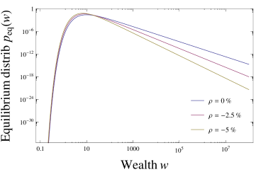
The equilibrium distribution $p_{\textrm{eq}}(w)$ for the stochastic model (7) is the inverse gamma distribution

$$p_{\textrm{eq}}(w)=\frac{\beta^{\alpha}e^{-\beta/w}}{\Gamma(\alpha)\,w^{\alpha+1}}$$ (40)

where $\alpha=1-2\rho/\sigma^{2}$ and $\beta=2l/\sigma^{2}$ (Fig. 6). Its differential entropy is given by

$$-\int_{0}^{\infty}p_{\textrm{eq}}(w)\log p_{\textrm{eq}}(w)\,dw=\frac{\alpha+\ln(2l/\sigma^{2})+\ln\Gamma(\alpha)-(1+\alpha)\psi(\alpha)}{\ln b},$$ (41)

where $\Gamma$ and $\psi$ and the gamma and digamma functions. Now, suppose that at time $t=0$, the effective return rate $\rho=\bar{r}-g-c$ changes to a different value $\rho^{\prime}=\rho+\delta\rho$. We can estimate the time before the the wealth distribution settles to a new equilibrium with tail exponent $\alpha^{\prime}=1-2\rho^{\prime}/\sigma^{2}$ as

$$\tau\simeq\left(\frac{\partial S_{\textrm{eq}}}{\partial\rho}\,\delta\rho\right)\Big{/}\left(\frac{dS_{t}}{dt}\right)\Big{|}_{t=0}.$$ (42)

From (41) we compute

$$\frac{\partial S_{\textrm{eq}}}{\partial\rho}=\left(\frac{-2}{\sigma^{2}}\right)\left(\frac{1-\psi_{1}(\alpha)(1+\alpha)}{\ln b}\right).$$ (43)

Next we estimate the denominator of (42) using

$$\frac{dS_{t}}{dt}\Big{|}_{t=0}\simeq\int_{0}^{\infty}P(w)\,j_{0}(w)dw.$$ (44)

where the initial flux $j_{0}(w)$ is given by

$$j_{0}(w) = (l+\rho^{\prime}w)p_{\textrm{eq}}(w)-\frac{\partial}{\partial w}\left(\frac{\sigma^{2}w^{2}p_{\textrm{eq}}}{2}\right)$$ (45)

$$= (l+\rho^{\prime}w)p_{\textrm{eq}}(w)-(l+\rho w)p_{\textrm{eq}}(w)$$ (46)

$$= (\delta\rho\,w)p_{\textrm{eq}}(w).$$ (47)

This gives

$$\frac{dS_{t}}{dt}\Big{|}_{t=0}\simeq\delta\rho\int_{0}^{\infty}wP(w)\,p_{\textrm{eq}}(w)dw.$$ (48)

The integral on the right-hand side can be evaluated explicited using (9) and (40), yielding

$$\int_{0}^{\infty}wP(w)\,p_{\textrm{eq}}(w)dw=\frac{1}{\ln b}.$$ (49)

Plugging (43) and (49) into (42) gives (16).

Appendix D Dictionary

Here we provide for the reader’s convenience a dictionary relating the concepts used in this paper, notably in sec. 2.3, to their physics counterparts.

Economics	Physics
Stratification	Gibbs entropy
Precariousness	(Driving force)/(temperature)
Mobility flux	Probability current
Potential	Potential energy
Surprisal	Stochastic or local entropy

References

- [1] H. Pringle, “The ancient roots of the 1%,” Science 344 no. 6186, (May, 2014) 822–825.
- [2] T. Piketty and E. Saez, “Inequality in the long run,” Science 344 no. 6186, (May, 2014) 838–843.
- [3] T. Piketty, Capital in the Twenty-First Century. Harvard University Press, Mar., 2014.
- [4] D. G. Champernowne, “A Model of Income Distribution,” Econ. J. 63 no. 250, (June, 1953) 318.
- [5] B. Mandelbrot, “The Pareto-Levy Law and the Distribution of Income,” International Economic Review 1 no. 2, (May, 1960) 79.
- [6] H. Kesten, “Random difference equations and Renewal theory for products of random matrices,” Acta Math. 131 no. 1, (Dec., 1973) 207–248.
- [7] J. Angle, “The Surplus Theory of Social Stratification and the Size Distribution of Personal Wealth,” Soc. Forces 65 no. 2, (Dec., 1986) 293–326.
- [8] S. Ispolatov, P. L. Krapivsky, and S. Redner, “Wealth distributions in asset exchange models,” The European Physical Journal B- … (1998) .
- [9] J.-P. Bouchaud and M. Mézard, “Wealth condensation in a simple model of economy,” Physica A 282 no. 3-4, (July, 2000) 536–545.
- [10] A. Dragulescu and V. M. Yakovenko, “Statistical mechanics of money,” Eur. Phys. J. B 17 no. 4, (Oct., 2000) 723–729.
- [11] M. Nirei, “Pareto Distributions in Economic Growth Models,” Tech. Rep. 09-05, 2009.
- [12] A. Chatterjee, S. Yarlagadda, and B. K. Chakrabarti, eds., Econophysics of Wealth Distributions. New Economic Windows. Springer Milan, Milano, 2005.
- [13] V. M. Yakovenko and J. B. Rosser Jr, “Colloquium: Statistical mechanics of money, wealth, and income,” Rev. Mod. Phys. (2009) .
- [14] J. Benhabib, A. Bisin, and S. Zhu, “The Distribution of Wealth and Fiscal Policy in Economies With Finitely Lived Agents,” Econometrica 79 no. 1, (Jan., 2011) 123–157.
- [15] P. Richmond, J. Mimkes, and S. Hutzler, Econophysics and Physical Economics. Oxford University Press, Sept., 2013.
- [16] A. Drăgulescu and V. M. Yakovenko, “Exponential and power-law probability distributions of wealth and income in the United Kingdom and the United States,” Physica A 299 no. 1-2, (Oct., 2001) 213–221.
- [17] A. Y. Abul-Magd, “Wealth distribution in an ancient Egyptian society,” Phys. Rev. E 66 no. 5, (Nov., 2002) 057104.
- [18] A. Atkinson, T. Piketty, and E. Saez, “Top Incomes in the Long Run of History,” tech. rep., National Bureau of Economic Research, Cambridge, MA, Cambridge, MA, Oct., 2009.
- [19] D. B. Grusky, Social Stratification. Class, Race, and Gender in Sociological Perspective. Westview Press, 2001.
- [20] U. Seifert, “Stochastic thermodynamics, fluctuation theorems, and molecular machines,” Rep. Prog. Phys. 75 (2012) 126001.
- [21] V. Mustonen and M. Lassig, “Fitness flux and ubiquity of adaptive evolution,” Proc. Natl. Acad. Sci. USA 107 no. 9, (Mar., 2010) 4248–4253.
- [22] J. L. England, “Statistical physics of self-replication,” J. Chem. Phys. 139 no. 12, (2013) 121923.
- [23] T. Piketty and G. Zucman, “Wealth and Inheritance in the Long Run,” in Handbook of Income Distribution. North Holland.
- [24] C. W. Gardiner, Handbook of Stochastic Methods for Physics, Chemistry, and the Natural Sciences. Springer Verlag, Jan., 2004.
- [25] X. Gabaix, “Power Laws in Economics and Finance,” Ann. Rev. Econ. 1 no. 1, (2009) 255–294.
- [26] B. M. Boghosian, “Kinetics of wealth and the Pareto law,” Phys. Rev. E 89 no. 4, (Apr., 2014) 042804.
- [27] J. L. Lebowitz and H. Spohn, “A Gallavotti-Cohen-Type Symmetry in the Large Deviation Functional for Stochastic Dynamics,” J. Stat. Phys. 95 no. 1/2, (1999) 333.
- [28] C. Maes, “On the origin and the use of fluctuation relations for the entropy,” Séminaire Poincaré 2 (2003) 29–62.
- [29] U. Seifert, “Entropy Production along a Stochastic Trajectory and an Integral Fluctuation Theorem,” Phys. Rev. Lett. 95 no. 4, (2005) 4.
- [30] B. Hayes, “Computing Science: Follow the Money,” American Scientist (2002) 400–405.
- [31] M. H. Cohen and I. I. Eliazar, “Econophysical visualization of Adam Smith’s invisible hand,” Physica A 392 no. 4, (Feb., 2013) 813–823.
- [32] C. Jarzynski, “Nonequilibrium work relations: foundations and applications,” Eur. Phys. J. B 64 no. 3-4, (July, 2008) 331–340.