Magnetomechanical response of bilayered magnetic elastomers

Abstract

Magnetic elastomers are appealing materials from an application point of view: they combine the mechanical softness and deformability of polymeric substances with the addressability by external magnetic fields. In this way, mechanical deformations can be reversibly induced and elastic moduli can be reversibly adjusted from outside. So far, mainly the behavior of single-component magnetic elastomers and ferrogels has been studied. Here, we go one step further and analyze the magnetoelastic response of a bilayered material composed of two different magnetic elastomers. It turns out that, under appropriate conditions, the bilayered magnetic elastomer can show a strongly amplified deformational response in comparison to a single-component material. Furthermore, a qualitatively opposite response can be obtained, i.e. a contraction along the magnetic field direction (as opposed to an elongation in the single-component case). We hope that our results will further stimulate experimental and theoretical investigations directly on bilayered magnetic elastomers, or, in a further hierarchical step, on bilayered units embedded in yet another polymeric matrix.

1 Introduction

The terms “magnetic hybrid materials” or “magnetic composite materials” are typically associated with classical magnetic elastomers or ferrogels [1]. These substances consist of a more or less chemically crosslinked and possibly swollen polymeric matrix into which paramagnetic, superparamagnetic, or ferromagnetic colloidal particles are embedded. In this way, the advantageous features of two different classes of materials are combined into one: on the one hand, one obtains free-standing soft elastic solids of typical polymeric properties [2, 3]; on the other hand, the materials can be addressed by external magnetic fields and in this way their properties can be tuned reversibly from outside as for conventional ferrofluids and magnetorheological fluids [4, 5, 6, 7, 8, 9, 10, 11, 12, 13, 14].

A lot of work has been spent on investigating how such ferrogels mechanically respond to external magnetic fields. In particular, these analyses focused on the nature of the induced shape changes [15, 16, 1, 17, 18, 19, 20, 21, 22, 23, 24, 25, 26, 27, 28, 29]. It turned out that the spatial distribution of the magnetic particles within a sample can qualitatively influence its response to the external field. This is because the magnetic interaction between the magnetic particles depends on their spatial arrangement. For example, when the particles were arranged on regular lattice structures, the system showed either an elongation along the external field or a contraction, depending on the particular lattice [19, 24, 29]. Likewise, anisotropic particle distributions and the presence of chain-like aggregates that can for example result from crosslinking the polymer matrix in the presence of a strong external magnetic field [30, 31, 32, 33, 34] can change the mechanical properties in and the deformational response to an external magnetic field [35, 1, 18, 20, 36, 27, 28]. Even the presence of randomly distributed dimer-like arrangements instead of single isolated magnetic particles was shown to be able to switch the distortion of a ferrogel from contractile along the field direction to extensile [22, 26].

The coupling of mechanical and deformational behavior to external magnetic fields, often referred to as “magnetomechanical coupling”, opens the way to various different types of application. Soft actuators [37] or magnetic sensors [38, 39] can be constructed that react mechanically to external magnetic fields or field gradients. Vibration absorbers [40] and damping devices [41] can be manufactured, the properties of which can be reversibly tuned from outside by applying an external magnetic field. In the search for an increased magnitude of magnetomechanical coupling, a new class of ferrogels was synthesized [42, 43]. Via surface functionalization of the magnetic particles, the polymer chains could be directly chemically attached to the particle surfaces. In this way, the magnetic particles became part of the embedding crosslinked polymer network. For such materials, a restoring mechanical torque acts on the particles when they rotate out of their initial orientations acquired during crosslinking [25], which constitutes a form of orientational memory [44].

Here we analyze a further type of magnetomechanical coupling that arises when layered materials of magnetic elastomers are considered. In our case, we investigate the deformational response of a bilayered magnetic elastomer to an external magnetic field combining phenomenological magnetostatics with elasticity theory. This type of deformation is related to the magnetic pressure on the material boundaries, similar to the Maxwell pressure in dielectrics. The boundary-related magnetic pressure acts not only on the outer surfaces of the sample, but also on the inner interfaces in the considered composite materials containing two (or many) layers of magnetic elastomers of different magnetic susceptibilities [45]. In conventional ferromagnetic materials this setup was for example suggested for sensor applications when two ferromagnetic prisms are separated by a piezolayer [46].

In this paper we theoretically analyze basic principles of the deformation in composite magnetic elastomers generated by the magnetic pressure of external fields. We connect the ultimate deformation of the composite material to the effective magnetic pole distribution on the material boundaries and at the bilayer interface. The material properties of the composite elastomer, such as its susceptibility and demagnetization coefficients, define a crucial parameter, called a geometrical function $A$, which plays a major role in the material reaction to the applied field. It turns out that, under appropriate conditions, the bilayered magnetic elastomer can show a strongly amplified deformational response in comparison to a single-component material. Furthermore, a qualitatively opposite response can be obtained, i.e. a contraction along the magnetic field direction (as opposed to an elongation in the single-component case).

The rest of the paper is organized as follows. In the next section the magnetic pressure on the particle boundaries and the geometry function $A$ are explained. The dependence of the function $A$ on the demagnetization coefficient $\alpha$ is discussed in section 3. In section 4 we investigate the magnetization of the different layers in the bilayer. The magnetic pole distribution and the expression for the elastic strain are discussed in section 5. Finally we conclude in section 6.

2 Magnetic energy density and magnetic driving pressure

When a homogeneous material with a magnetic permittivity $\mu$ is placed into a uniform external magnetic field $\vec{H}_{0}$, the driving pressure on the material boundary is associated with the difference between the relative energy densities

$$\Delta u=\frac{\mu H^{2}}{2}-\frac{\mu_{0}H_{0}^{2}}{2}.$$ (1)

Here $\mu_{0}$ is the susceptibility of vacuum, $\mu_{0}=1.26\times 10^{-6}$ $\frac{mkg}{s^{2}A^{2}}$, and $H$ denotes the internal magnetic field. Using the relation between the magnetization $M$ and the internal field $H$ in an isotropic material,

$$M=\chi H,$$ (2)

where $\chi$ is the susceptibility of the material, and

$$H=\frac{H_{0}}{1+\alpha\chi}$$ (3)

is the internal field in the material. Here, $\alpha$ is the demagnetization coefficient of the sample along the field direction $\vec{z}$. Assuming a rectangular prism geometry for the material, the full energy difference can be rewritten as

$$\Delta U=V\Delta u=\frac{\mu_{0}MH_{0}}{2}A(\alpha,\chi)\,V.$$ (4)

Here $V=L^{2}L_{z}$ is the volume of the material, with $L_{z}$ the edge length of the sample along the field direction $\vec{z}$, and $L$ the edge lengths in the remaining lateral directions set equal for simplicity. The demagnetization coefficient $\alpha$ depends on the dimensional lengths of the sample. In general, the factor $\alpha^{(l)}$ has $l=x,y,z$ components, which obey $\sum_{l}\alpha^{(l)}=1$. Whereas for simple geometrical shapes the coefficients $\alpha^{(l)}$ are well known, for example, for a sphere and a cube $\alpha^{(x)}=\alpha^{(y)}=\alpha^{(z)}=1/3$, and for a slab with infinite lateral $(xy)$ dimensions $\alpha^{(x)}=\alpha^{(y)}=0$, and $\alpha^{(z)}=1$, for the rectangular prisms considered in this work the coefficients $\alpha^{(l)}$ are not known apriori. Their values, however, can be calculated using analytical expressions given in Ref. [47, 48], or taken from the tabulated results available in Ref. [49]. In the following we will adopt the notion $\alpha=\alpha^{(z)}$.

The geometry factor $A(\alpha,\chi)$ in Eq.(4) turns out to be

$$A(\alpha,\chi)=\frac{1-2\alpha-\alpha^{2}\chi}{1+\alpha\chi}$$ (5)

and obeys $|A(\alpha,\chi)|\leq 1$. This function defines the type of the deformation: a positive $A(\alpha,\chi)$ means a stretching, and a negative $A(\alpha,\chi)$ means a compression of the material along the applied field. A full description of this function is presented in section 3.

Under the driving pressure the material is deformed because of the propagation of the material boundary from the area with high susceptibility into the surrounding area with low susceptibility. The deformational changes of the material, namely the changes in its thickness $L_{z}$ and area $S=L^{2}$, lead to the magnetic energy difference in Eq.(4)

$$\Delta U=\frac{\partial U}{\partial L_{z}}\Delta L_{z}+\frac{\partial U}{\partial S}\Delta S.$$ (6)

Assuming that the density of the material does not change during this type of deformation, which is referred to as a constant volume condition, written as

$$SL_{z}=(S+\Delta S)(L_{z}-\Delta L_{z}),$$ (7)

we get the following relation between $\Delta S$ and $\Delta L_{z}$ when $\Delta L_{z}/L_{z}\ll$1

$$\Delta S=S\frac{\Delta L_{z}}{L_{z}}$$ (8)

From Eq.(4), assuming that neither $M$ nor $H$ strongly depend on the changes in the material geometry, which is valid only for small shape deformations, for the partial derivatives of the stored energy we find

$$\frac{\partial U}{\partial L_{z}}=\frac{1}{2}\mu_{0}H_{0}MSA(\alpha,\chi)\,\,,$$

$$\frac{\partial U}{\partial S}=\frac{1}{2}\mu_{0}H_{0}ML_{z}A(\alpha,\chi).$$ (9)

Inserting Eq.(9) into Eq.(6) and using Eq.(8) we obtain

$$\Delta U=\mu_{0}H_{0}MS\Delta L_{z}\,A(\alpha,\chi).$$ (10)

Taking into account the force-energy relation $F=\Delta U/\Delta L_{z}$, we obtain the final expression for the magnetic pressure,

$$p=|\vec{F}|/S=\mu_{0}|\vec{H}_{0}|A(\alpha,\chi)(\vec{M}\cdot\vec{n}).$$ (11)

Here $\vec{n}$ is a unit vector normal to the material surface pointing outward the sample surface. It should be noted that for specific cases when the constant volume condition Eq.(7) does not apply, for example, in magnetic liquids which can leave the field area when squeezed by magnetic forces, the second term containing $\Delta S$ in Eq.(6) can be zero. For such cases the magnetic pressure will be half the pressure defined by Eq.(11).

The term $\vec{M}\cdot\vec{n}$ in Eq.(11) defines the effective magnetic pole density [50]

$$\sigma_{M}=\vec{M}\cdot\vec{n}$$ (12)

at the boundaries of the sample. The sign of these magnetic poles is positive on the upper boundary, and negative on the bottom boundary of the sample if the field direction is from the bottom to the top.

3 Geometry-dependent deformation under an applied field

It is evident from Eq.(11) that the magnetic driving force $\vec{F}$ acts on the upper and bottom surfaces in opposite directions trying to stretch the prism if $A(\alpha,\chi)$ is positive. In the opposite case, when $A(\alpha,\chi)$ is negative, the driving force $\vec{F}$ pushes the upper and bottom boundaries towards each other.

The limiting boundaries of $A(\alpha,\chi)$ are dictated by the dependence of the coefficient $\alpha$ on the geometry of the material. For an infinite slab with $L_{z}/L\to 0$ and $\alpha\approx 1$ the function $A$ reaches its bottom limit $A(\alpha,\chi)\approx-1$ from Eq.(5), which recovers the classical relation $u=-\mu_{0}MH_{0}/2$ for the magnetic energy density [51]. Putting $\alpha=0$ (the case of an elongated cylinder along the $z$-axis) into Eq.(5) we get the upper limit for $A(\alpha,\chi)=1$. The function $A(\alpha,\chi)$ changes its sign at $\alpha=\sqrt{1+\chi}-1$, as shown in Figure 1. The zeros of $A$ correspond to the particular dimensions of the prism at which no deformation of the material is observed.

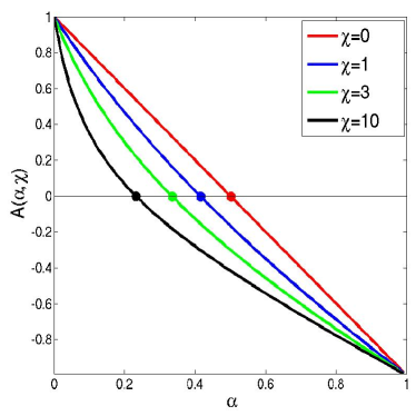
Figure 1: (Color in online) Geometrical factor $A(\alpha,\chi)$ for four different values of the magnetic susceptibility $\chi$. Note that the zeros of $A$ correspond to the particular dimensions of the prism at which no deformation of the material is observed.

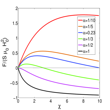
Figure 2: (Color in online) Normalized pressure $F/(S\mu_{0}H_{0}^{2})$ as a function of the magnetic susceptibility $\chi$ for six different values of $\alpha$. Note that the force becomes completely positive at $\alpha<0.23$, and completely negative at $\alpha>0.5$. $F>0$ corresponds to an elongation along the magnetic field direction, whereas $F<0$ implies a contraction.

For the case $0<\chi<10$ considered in this paper, the function $A(\alpha,\chi)$ is always positive for $\alpha<0.23$, which corresponds roughly to the size ratio $L_{z}/L>3.3$. An opposite scenario, a shrinking of the prism for all $0<\chi<10$ is predicted for $\alpha>0.5$ which roughly corresponds to the size ratio $L_{z}/L<1.4$. This is demonstrated in Figure 2 where the magnetic pressure $F/S$ is plotted against the susceptibility $\chi$.

4 Magnetization of a magnetic bilayer under external field

We now consider a composite bilayered magnetic elastomer of a rectangular shape with a 2-2 connectivity [52] as shown in Figure 3. The rectangular prism has dimensions $L_{x},L_{y},L_{z}$, and for simplicity we assume that its lateral dimensions are the same, $L_{x}=L_{y}=L$. The bottom and upper parts of the prism, denoted as layers i=1 and i=2, are made from different materials with magnetic susceptibilities $\mu_{1}$ and $\mu_{2}$, and elastic moduli $Y_{1}$ and $Y_{2}$, and have thicknesses $d_{1}$ and $d_{2}=L_{z}-d_{1}$ correspondingly. There is no gap between the layers of the prism, $d=0$, hence the stacking density of the composite is $\rho=L_{z}/(d+L_{z})=1$.

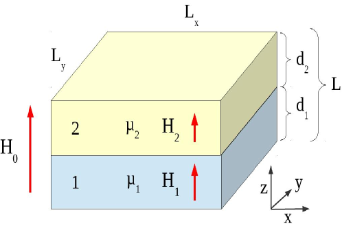
Figure 3: (Color in online) Schematic illustration of the composite bilayered magnetic elastomer in the form of a prism with 2-2 connectivity under an external magnetic field $H_{0}$.

When an external magnetic field $\vec{B}_{0}=\mu_{0}\vec{H}_{0}$ is applied along the $z$-axis, $\vec{H}_{0}\parallel\vec{z}$, the field $\vec{B}_{i}$ in the layer $i$ is determined as

$$\vec{B}_{i}=\mu_{0}(\vec{H}_{i}+\chi_{i}\vec{H}_{i})$$ (13)

where the magnetic field $\vec{H}_{i}$ is defined as

$$\vec{H}_{i}=\vec{H}_{0}+\vec{H}_{d}^{(i)}+\vec{R}_{i}(\vec{H}_{j}).$$ (14)

Here $\vec{H}_{d}^{(i)}$ is a demagnetization field in the prism $i$ [53]. This field originates from the existence of magnetic poles at the boundaries of the prism $i$ perpendicular to the field, in analogy to the polarization charges at the dielectric boundaries under an external electric field. In the linear response theory the field $\vec{H}_{d}^{(i)}$ reads

$$\vec{H}_{d}^{(i)}=-\alpha_{i}\vec{M}_{i},$$ (15)

where $\alpha_{i}$ is the demagnetization factor of the prism $i$ along the $z$-axis.

The last term on the right hand side of Eq.(14), $\vec{R}_{i}(\vec{H}_{j})$, represents the average value of the magnetic field $\vec{H}_{j}$ generated by the magnetized layer $j$ in the volume of layer $i$, where $j\neq i$. The full distribution of this cross field can be calculated using numerical methods, see Ref. [54]. The field $\vec{R}_{1}(\vec{H}_{2})$, schematically drawn in Figure 4, is inhomogeneous along the $z$-axis: it has a maximum value at the top of the layer 1 and becomes weaker towards the bottom edge of the layer 1. There are different approaches about accepting the best approximation for $R_{i}$, see Ref. [55]. The so-called ’ballistic’ approach defines $\vec{R}_{i}$ as the averaged $\vec{R}_{i}(\vec{H}_{2})$ in the $xy$ mid-plane of layer 1. Or, the ’local’ approach defines $\vec{R}_{i}(\vec{H}_{2},z)$ along the central line $z$ with $x=y=0$. Within the ’side’ approach $\vec{R}_{i}$ is measured as an averaged field over the surfaces of the layer $i$ perpendicular to $z$. In our generalized approach we assume that the average field $\vec{R}_{i}$ is homogeneous across the layer $i$ and is a fraction of the magnetization of layer j,

$$\vec{R}_{i}=\gamma_{i}\vec{M}_{j}.$$ (16)

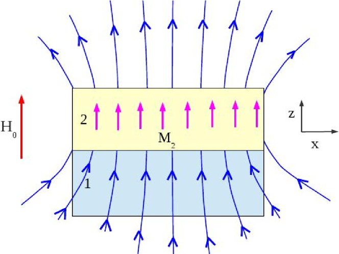
Figure 4: (Color in online) Schematic presentation of the cross term $\vec{R}_{1}(\vec{H}_{2})$, which corresponds to the field lines generated by $\vec{M}_{2}$ of layer 2 in the volume of layer 1.

The connectivity coefficient $\gamma_{i}$ can be easily defined from the boundary condition for the magnetic field $\vec{B}$ assuming that there is no external field, $H_{0}=0$, and a permanently magnetized layer $j$ is the only source that generates a magnetic field in the layer $i$. For $i=1$ and $j=2$, the case shown in Figure 4, the field inside layer 2 is

$$\vec{B}_{2}=\mu_{0}(\vec{H}_{2}+\vec{M}_{2}).$$ (17)

Outside layer 2, at its bottom boundary,

$$\vec{B}_{out}=\mu_{0}\vec{H}_{out},$$ (18)

Putting

$$\vec{H}_{2}=\vec{H}_{0}-\alpha_{2}\vec{M}_{2}=-\alpha_{2}\vec{M}_{2}$$ (19)

into Eq.(17), we get

$$\vec{B}_{2}=\mu_{0}(1-\alpha_{2})\vec{M}_{2}.$$ (20)

Applying the boundary condition for the continuity of the perpendicular component of $\vec{B}$ at the bottom boundary of layer 2, $\vec{B}_{out}=\vec{B}_{2}$, we get from Eq.(18) and Eq.(20)

$$\vec{H}_{out}=(1-\alpha_{2})\vec{M}_{2}.$$ (21)

Within the ”upper side” approach $R_{1}=H_{out}$, and using Eq.(16) and Eq.(21) we arrive at the preliminary connectivity coefficient

$$\widetilde{\gamma_{1}}=1-\alpha_{2}.$$ (22)

However, within our generalized approach $R_{1}<H_{out}$, and thus using $R_{1}=\beta_{1}H_{out}$, where $\beta_{1}<1$ is a coefficient that, generally speaking, depends on the coefficients $\alpha_{1}$ and $\alpha_{2}$, we get for the connectivity coefficient

$$\gamma_{1}=\beta_{1}(1-\alpha_{2}).$$ (23)

The exact value of $\beta_{1}$ can be calculated only using numerical procedures. In our analytical approach we can define the upper limit for $\beta_{1}$, above which non-physical effects of negative magnetization might take place, see Appendix A for more details.

In a similar manner we define the connectivity coefficient for the second layer as $\gamma_{2}=\beta_{2}(1-\alpha_{1})$. It is worth to mention that, for an infinitely wide ($L\gg L_{z}$) prism $\alpha_{i}=1$ ($i$=1,2), and the connectivity coefficients $\gamma_{i}=0$ regardless of the values of $\beta_{i}$, meaning that $R_{i}(H_{j})=0$. In other words, the cross term $R_{i}(H_{j})$ is negligible for flat geometries.

Finally we arrive at the following relation for the field $\vec{H}_{i}$ inside the layer $i$ of the prism placed under the external field $\vec{H}_{0}$,

$$\vec{H}_{1}=\vec{H}_{0}-\alpha_{1}\vec{M}_{1}+\beta_{1}(1-\alpha_{2})\vec{M}_{2},$$

$$\vec{H}_{2}=\vec{H}_{0}-\alpha_{2}\vec{M}_{2}+\beta_{2}(1-\alpha_{1})\vec{M}_{1}.$$ (24)

Below, for simplicity, we will assume that $\beta_{1}=\beta_{2}=\beta$ in order to proceed to analytical results. Thus putting $\vec{H}_{i}=\vec{M}_{i}/\chi_{i}$, where $\chi_{i}$ is the susceptibility of the layer $i$ we find

$$M_{1}=H_{0}\frac{\chi_{1}(1+\alpha_{2}\chi_{2})+\beta\chi_{1}\chi_{2}(1-\alpha_{2})}{(1+\chi_{1}\alpha_{1})(1+\chi_{2}\alpha_{2})-\beta^{2}(1-\alpha_{1})(1-\alpha_{2})\chi_{1}\chi_{2}},$$

$$M_{2}=H_{0}\frac{\chi_{2}(1+\alpha_{1}\chi_{1})+\beta\chi_{1}\chi_{2}(1-\alpha_{1})}{(1+\chi_{1}\alpha_{1})(1+\chi_{2}\alpha_{2})-\beta^{2}(1-\alpha_{1})(1-\alpha_{2})\chi_{1}\chi_{2}}.$$ (25)

For a single layer, i.e. when $\chi_{2}=0$, from Eq.(25) we recover the magnetization $M_{1}$ of the single layer

$$\vec{M}_{1}=\vec{H}_{0}\frac{\chi_{1}}{1+\alpha_{1}\chi_{1}}.$$ (26)

Eq.(25) is the main result for the magnetization of the bilayer and will be used to calculate the magnetic pressure on the composite prism in the next section.

5 Magnetic pole distribution at the bilayer interface

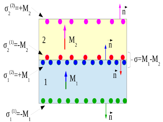
Figure 5: (Color in online) Distribution of the magnetic poles at the prism boundaries. The sign of the poles is defined from $\sigma_{i}^{(j)}=\left(\vec{M}_{i}\cdot\vec{n}\right)_{j}$, where $j$ indicates the bottom ($j=1$) and upper ($j=2$) boundaries of each layer $i=1,2$. $\vec{n}$ is a unit vector pointing outward from the layer surface.

For the set-up presented in Figure 3 the distribution of the poles is schematically shown in Figure 5. For the pole density on layer 1 we have $\sigma_{1}^{(1)}=-M_{1}$ for the bottom and $\sigma_{1}^{(2)}=+M_{1}$ for the top boundaries, and for layer 2 the density of boundary poles are $\sigma_{2}^{(1)}=-M_{2}$ and $\sigma_{2}^{(1)}=+M_{2}$ correspondingly. As a result, the net magnetic pole density at the interface between layers 1 and 2 is

$$\Delta\sigma=\sigma_{1}^{(2)}+\sigma_{2}^{(1)}=M_{1}-M_{2},$$ (27)

or, taking into account Eq.(25),

$$\Delta\sigma=H_{0}\frac{\chi_{1}-\chi_{2}+(\alpha_{1}-\alpha_{2})(1-\beta)\chi_{1}\chi_{2}}{(1+\chi_{1}\alpha_{1})(1+\chi_{2}\alpha_{2})-\beta^{2}(1-\alpha_{1})(1-\alpha_{2})\chi_{1}\chi_{2}}.$$ (28)

From Eq.(11) for the driving pressure $p=\frac{F}{S}=\frac{F_{1}-F_{2}}{S}$ acting on the interface 1-2 we have

$$p=\mu_{0}|\vec{H}_{0}|\left[A(\alpha_{1},\chi_{1})\vec{M}_{1}-A(\alpha_{2},\chi_{2})\vec{M}_{2}\right]\cdot\vec{n}.$$ (29)

This expression reduces to a simple form

$$p=\mu_{0}|\vec{H}_{0}|A(\alpha)\Delta\sigma$$ (30)

for $\alpha_{1}=\alpha_{2}=\alpha$, $\chi_{1}\ll 1$, and $\chi_{2}\ll 1$, hence $A(\alpha)=(1-2\alpha)$. A positive (negative) $p$ in Eq.(29) and Eq.(30) means that the layer 1 will be stretched (squeezed) into the layer 2, whereas the layer 2 will be squeezed (stretched).

As has been mentioned in section 2, both the thickness $L_{z}$ and the area $S$ of the prism deform under the constant volume condition. The total change $\Delta L_{z}$ of the bilayer thickness is a sum of the thickness changes in each layer,

$$\Delta L_{z}=\sum_{i=1}^{2}\Delta d_{i},$$ (31)

where $\Delta d_{i}$ is defined through Hooke’s relation for the boundary forces $F_{1}$ and $F_{2}$,

$$\,\,\,\,\,F+F_{1}=SY_{1}\frac{\Delta d_{1}}{d_{1}},$$

$$-F+F_{2}=SY_{2}\frac{\Delta d_{2}}{d_{2}},$$ (32)

where $F_{i}$, $i=1,2$ is given by Eq.(11).

Putting everything together we have for the strain $\Sigma_{B}=\Delta L_{z}/L_{z}$,

$$\Sigma_{B}=\frac{d_{1}}{L_{z}}\left(\frac{F+F_{1}}{SY_{1}}+\frac{F-F_{2}}{SY_{2}}\right)+\frac{F_{2}-F}{SY_{2}}.$$ (33)

This expression, together with the definitions for the forces $F_{i}$

$$\frac{F_{i}}{S}=\mu_{0}|\vec{H}_{0}|A(\alpha_{i},\chi_{i})(\vec{M}_{i}\cdot\vec{n})$$ (34)

and the magnetization $M_{i}$ defined by Eq.(25) constitute our main result for the reaction of the bilayered magnetic elastomer to the applied field $H_{0}$. Note that whereas the pole distribution term $(\vec{M}_{i}\cdot\vec{n})$ and the geometry factor $A(\alpha_{i},\chi_{i})$ in the magnetic pressure equation Eq.(34) together determine the magnetic force on the layer i due to the external field, the total deformation of the layer i is regulated by the forces given in Eq.(32)

6 Results

The strain $\Sigma_{B}$ in Eq.(33) depends on the forces $F_{i}$, the conformation parameter $x=d_{1}/L_{z}$, and the elasticity moduli $Y_{i}$. The forces $F_{i}$, according to Eq.(25) and Eq.(34), are also functions of the four parameters $\alpha_{1}$, $\alpha_{2}$ and $\chi_{1}$, $\chi_{2}$:

$$F_{i}=F_{i}(\alpha_{1},\chi_{1},\alpha_{2},\chi_{2}).$$

In total, the strain $\Sigma_{B}$ depends on the six parameters making the analyses of the strain $\Sigma_{B}$ a very complicated task. However, a consideration of the relative strain, defined as

$$\Sigma=\Sigma_{B}/\Sigma_{S},$$ (36)

where the single layer strain is

$$\Sigma_{S}=\frac{F_{3}}{SY_{2}}$$ (37)

(assuming that the single layer is made of material 2, has the same thickness $L_{z}$ as the composite prism, and $F_{3}/S$ is the magnetic pressure acting on this single-layered reference sample under an identical external magnetic field), brings the number of independent system parameters from six down to four.

6.1 Relative strain of the bilayered composite

The relative strain $\Sigma$ in Eq.(36) measures how effective the reaction of the bilayered structure to the applied field is, and can be rewritten in parametric form as

$$\Sigma=(1-x)\left(2\theta-\frac{f}{2}\right)+(2f-\theta)\frac{x}{y}.$$ (38)

Here we have adopted $f=\frac{F_{1}}{F_{3}}$, $y=\frac{Y_{1}}{Y_{2}}$, $x=\frac{d_{1}}{L_{z}}$, and $\theta=F_{2}/F_{3}$. The strain $\Sigma$ now depends on four variables instead of six variables for $\Sigma_{B}$, which makes its analyses relatively simple. We can fix $\theta$ and $x$, and explore the dependence of $\Sigma$ on the parameters $y$ and $f$.

The most interesting cases are
(i) $\Sigma>1$, the case of strong bilayer stretching (squeezing) relative to the single layer stretching (squeezing), and
(ii) $\Sigma<0$, the case of bilayer shrinking (stretching) while the single layer stretches (shrinks).

The case $0<\Sigma<1$ corresponds to a weak bilayer reaction and thus is not interesting to us. The parameters $f$ and $\theta$ can run between $-\infty$ and $+\infty$, but for simplicity we will restrict ourselves to considering $f>1$ and $\theta>1$, which corresponds either to the case when $F_{1}>F_{3}$, $F_{2}>F_{3}$, as well as $F_{3}>0$, or to the case $F_{1}<F_{3}$, $F_{2}<F_{3}$, as well as $F_{3}<0$.

From Eq.(38) for $\Sigma>1$ we have the following relation for $y(f)$:

$$y<\frac{x(2f-\theta)}{1-(1-x)(2\theta-f/2)}.$$ (39)

Similarly, the condition $\Sigma<0$ leads to the following relation

$$y>\frac{x(2f-\theta)}{(1-x)(f/2-2\theta)}.$$ (40)

Representative pictures for both of these curves, Eq.(39) and Eq.(40), and for $\theta=1$ are shown in Figure 6. It is evident that as the composition factor $x$ increases, a transition from strong stretching ($\Sigma>1$) to squeezing ($\Sigma<0$) appears at high $y$ values. Also, the area of the weak reaction, $0<\Sigma<1$, widens as the composition factor $x$ increases.

The 3D pictures for the relative strain, plotted in Figure 7, show that a mild stretching and a strong squeezing at low $x$ is replaced by the strong stretching and the weak squeezing at large $x$.

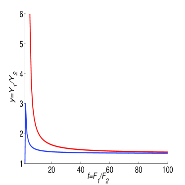
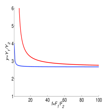
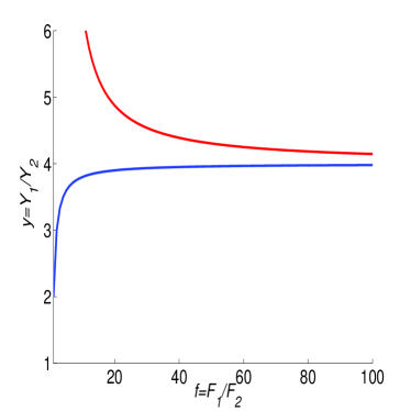
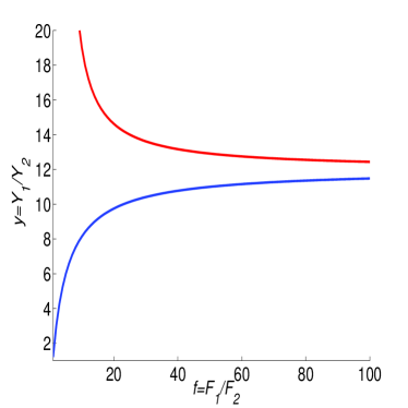
Figure 6: (Color in online) Logarithmic plot for relative strain curves corresponding to Eq.(39) and Eq.(40) for the composition parameter $x=0.25$ (a), $x=0.4$ (b), $x=0.5$ (c), $x=0.75$ (d). Dashed line (red in color) corresponds to $\Sigma=0$, solid line (blue in color) is for $\Sigma=1$. Above the dashed line $\Sigma<0$, and below the solid line $\Sigma>1$. In the area between these two lines $0<\Sigma<1$.

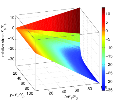
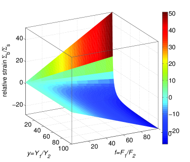
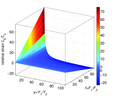
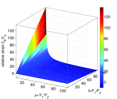
Figure 7: (Color in online) 3D pictures for the relative strain $\Sigma$ as a function of the parameters $y$ and $f$ from Eq.(38) and for the composition parameter $x=0.25$ (a), $x=0.4$ (b), $x=0.5$ (c), $x=0.75$ (d). The color code from dark red to dark blue corresponds to a decreasing strain strength.

6.2 Full strain of the bilayer composite

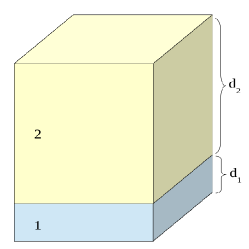
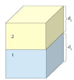
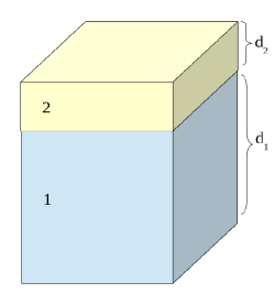
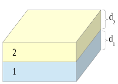
Figure 8: (Color in online) Geometrical illustration for the 4 different setups from Table 1. Upper row: Setups 1, 2, and 3; bottom row: Setup 4.

In this section we analyze the full strain of the bilayer $\Sigma_{B}$ given by Eq.(33). We consider three representative cases for $x$, namely $x=0.25,\,0.5,\,0.75$. Four different setup configurations with the corresponding parameters $\alpha_{i}$ and $A(\alpha_{i},\chi_{i})$ are shown in Table 1. These setups cover the cases when the coefficients $A(\alpha_{i},\chi_{i})$ are simultaneously either positive or negative, or have opposite signs. Corresponding setup configurations are graphically presented in Figure 8.

Table 1: Geometry-defined demagnetization coefficients $\alpha_{i}$ and the geometry functions $A(\alpha_{i},\chi_{i})$ for the three composition parameters $x$ describing the four different setups in Figure 8. $\chi_{1}=1$ and $\chi_{2}=10^{-3}$ were used to calculate $A(\alpha_{i},\chi_{i})$.

Setup	$x$	$\alpha_{1}$	$\alpha_{2}$	$A(\alpha_{1},\chi_{1})$	$A(\alpha_{2},\chi_{2})$
1	0.25	$\frac{2}{3}$	$\frac{1}{10}$	-0.47	0.8
2	0.5	$\frac{1}{3}$	$\frac{1}{3}$	0.25	0.33
3	0.75	$\frac{1}{10}$	$\frac{2}{3}$	0.72	-0.33
4	0.5	$\frac{2}{3}$	$\frac{2}{3}$	-0.47	-0.33

The bilayer strain for Setup 1 as a function of parameters $\chi=\chi_{1}/\chi_{2}$ and $y=Y_{1}/Y_{2}$ is plotted in Figure 9a. For this case the bilayer has a completely positive deformation, meaning that it always experiences a stretching. A relatively high deformation at fixed $y$ happens at larger values of $\chi$. If an imaginary line at fixed $y=10^{4}$ is followed from $\chi=1$ to $\chi=10^{6}$, the composite strain will increase gradually from zero to several percents achieving a value of about 10 % at $\chi>10^{5}$.

A completely different scenario is observed for Setup 2 with $x=0.5$, see Figure 9b. In this equivalent case when the layers have the same thicknesses $d_{1}=d_{2}$, the strain shows both negative and positive domains. The black line corresponds to $\Sigma_{B}=0$, a zero deformation of the composite for $\Delta L_{z}$=0. This zero strain happens when the changes in the layer $1$ and layer $2$ thicknesses compensate each-other, $\Delta L_{1}=-\Delta L_{2}$. A negative strain, or a shrinking of the bilayer along the $z$-axis, takes place at high $\chi$ and low $y$ values. Another negative strain region is visible for $\chi<10^{3}$ and at about $y>2$. Also, in addition to the strong stretching similar to the Setup 1, there is the second, though very mild, stretching in the very tiny strip at low $\chi$ and the $y$ stripes around the bottom left corner of the left plot in Figure 9b. If an imaginary line at fixed $y=10^{4}$ is followed from $\chi=1$ to $\chi=10^{6}$, the composite deformation will be first positive, then negative, and then positive again. Thus the positive deformation of the composite is reentrant as a function of $\chi$.

In Setup 3 we again observe two positive and two negative deformation domains, see Figure 9c. However, the overall picture is totally different from the results for Setups 1 and 2. First, the areas of strong stretching for previous setups now show a small stretching less than a few percents. Second, the shrinking of the composite increases, reaching $-15$ %, wheres in Setup 2 it was around $-6$ %. Third, a visible negative well develops for $10^{2}<\chi<10^{5}$. And fourth, a strong stretching is visible at very small $y$ around $\chi\approx 10^{4}$. If we again follow an imaginary line at fixed $y=10^{4}$ and from $\chi=1$ to $\chi=10^{6}$, the composite deformation will first be negative, then becomes more negative, and then positive.

Setup 4 has the same composition factor $x=0.5$ as the Setup 2. The only difference between these Setups is the fact that in the former case both geometry functions are negative, while in the latter case they are positive. As seen from Figure 9d, here we only have a single positive and a single negative strain domain. Basically the strain maximum and minimum values stay the same as for Setup 2, but now the low $\chi$ stripe at the left bottom corner of Figure  9d is negative. Again, if an imaginary line at fixed $y=10^{4}$ is followed from $\chi=1$ to $\chi=10^{6}$, the composite deformation will first be negative and then positive.

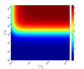
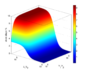
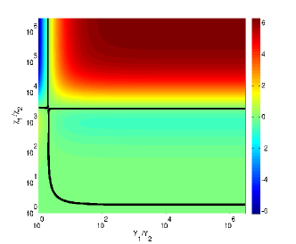
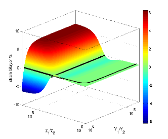
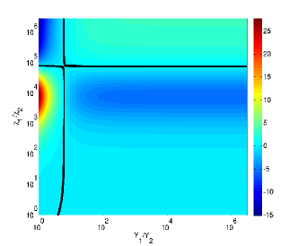
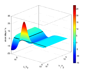
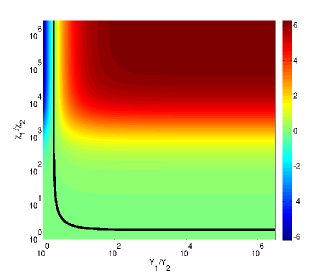
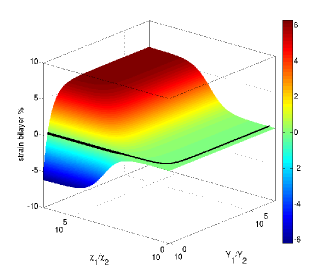
Figure 9: (Color in online) Logarithmic plot for the bilayer strain from the four Setups given in Table 1. From top to bottom, Setup 1 (a), Setup 2 (b), Setup 3 (c), and Setup 4 (d). The other system parameters are: $L=100\mu m$, $L_{z}=200\mu m$, $\chi_{2}=10^{-3}$, $Y_{2}=10^{5}\frac{N}{m^{2}}$, $B_{0}=\mu_{0}H_{0}=0.13$ Tesla. The left picture corresponds to the top view of the 3D surface that is shown on the right. Black lines indicate a zero strain of the composite, $\Sigma_{B}=0$. The color code from dark red to dark blue corresponds to a decreasing strain strength.

7 Conclusions

As explained in the introduction, there are different sources of magnetomechanical coupling in ferrogels and magnetic elastomers. The most obvious one is associated with the magnetic interactions between embedded magnetic particles, which can induce mechanical deformations [19, 20, 21, 22, 24, 25, 26, 23, 27, 28, 29]. Furthermore, the aligning magnetic torque onto embedded ferromagnetic particles can directly induce distortions when the particles are chemically crosslinked into the polymer mesh [42, 43, 25].

In this paper, we have analyzed a completely different source of magnetomechanical coupling. It results from the structural arrangement of two magnetic elastomers into a bilayered composite material. More technically speaking, it follows from the interplay of the magnetic pressures acting on the outer boundaries of the sample and on the internal interfacial boundaries between the layers.

Using linear response theory for the magnetization and demagnetization fields of a composite material of a rectangular prism geometry, we have defined the strain of the bilayer structure to the applied field. We have connected the ultimate deformation of the sample to the magnetic pole distribution on the outer boundaries and at the bilayer interface. The material properties of the composite particle, such as its susceptibilities and demagnetization coefficients, define a crucial parameter, called the geometrical function $A$, which plays a major role in the reaction to the applied field. According to our results, the composite magnetic elastomer is able to respond more efficiently to the external field in comparison to a single-component material. This response also strongly depends on the composition factor of the sample. By changing the composition factor $x=d_{1}/L_{z}$ of the bilayer, it is possible to shift from a mostly stretching composite to a mostly squeezing one when all other material parameters are kept fixed.

Our results are important for the design of optimized bilayered composites of magnetic elastomers and gels. We hope that our analysis will stimulate further research in this direction, both experimentally and theoretically. Nevertheless, we are already thinking one step further in a structural hierarchy of magnetic elastomers. Just like magnetic particles embedded in a surrounding polymer matrix in magnetic elastomers or ferrogels, we intend to consider on an upper hierarchical level units of bilayered magnetic elastomers embedded in yet another non-magnetic polymeric matrix.

Obviously, when the bilayered units stretch along an external magnetic field, the overall hierarchical material will elongate along the applied field and get squeezed perpendicular to it due to volume conservation. In the opposite case, when the bilayered units squeeze along the field direction, the overall sample will extend perpendicularly to the field, and its shrinking will be along the field. The right management of differently shaped or differently composed bilayered units and the right regulation of their embedding places in the overall sample can adjust its overall deformation to the needed demand. For example, it is possible to heterogeneously tune the response of the system during synthesis, making it elongate in one part and at the same time shrink in another part. All these effects are potentially interesting for their application in a new generation of sensors and in creating new smart (intelligent) materials.

Appendix A Field correction coefficient $\beta$

The meaning of the coefficient $\beta$ is obvious from the relation between the magnetization $M$ and the external field $H_{0}$ in magnetic gels: the magnetization should have the same direction as the applied field. As shown in Figure 10, where the magnetization $M_{1}$ of layer 1 is plotted as a function of its susceptibility $\chi_{1}$ for the different values of $\beta$, at some $\beta$ a pole develops in Eq.(25). The pole causes a nonphysical flipping over of the magnetization vector $\vec{M}_{1}$. Decreasing the value of $\beta$ guarantees the “correct” behavior of $\vec{M}_{1}$. All the setup configurations used in the main text are free from such pole effect for the values of $\beta\leq 1$. Physically, the factor $\beta$ contains the widening of the field lines away from the interfacial boundary of layer 2, see Figure 4.

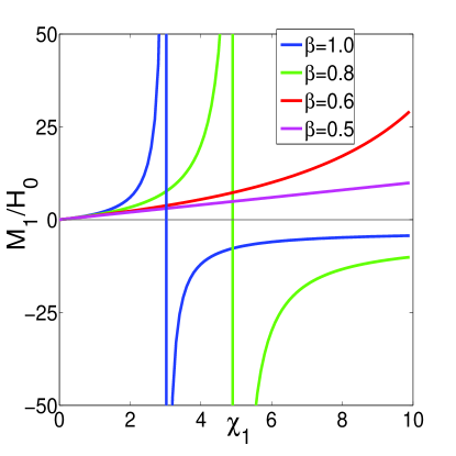
Figure 10: (Color in online) The magnetization $\vec{M}_{1}$ of layer 1 depends on the parameter $\beta$. Other parameters: $\chi_{1}=\chi_{2}$, $\alpha_{1}=\alpha_{2}=1/3$.

References

- [1] G. Filipcsei, I. Csetneki, A. Szilágyi, and M. Zrínyi. Magnetic field-responsive smart polymer composites. Adv. Polym. Sci., 206:137–189, 2007.
- [2] M. Doi and S. F. Edwards. The Theory of Polymer Dynamics. Clarendon Press, Oxford, 1988.
- [3] G. Strobl. The Physics of Polymers. Springer, Berlin/Heidelberg, 2007.
- [4] R. E. Rosensweig. Ferrohydrodynamics. Cambridge University Press, Cambridge, 1985.
- [5] S. Odenbach. Ferrofluids–magnetically controlled suspensions. Colloid Surface A, 217(1–3):171–178, 2003.
- [6] S. Odenbach. Magnetoviscous effects in ferrofluids. Springer, Berlin/Heidelberg, 2003.
- [7] B. Huke and M. Lücke. Magnetic properties of colloidal suspensions of interacting magnetic particles. Rep. Prog. Phys., 67(10):1731–1768, 2004.
- [8] S. Odenbach. Recent progress in magnetic fluid research. J. Phys.: Condens. Matter, 16:R1135–R1150, 2004.
- [9] B. Fischer, B. Huke, M. Lücke, and R. Hempelmann. Brownian relaxation of magnetic colloids. J. Magn. Magn. Mater., 289:74–77, 2005.
- [10] P. Ilg, M. Kröger, and S. Hess. Structure and rheology of model-ferrofluids under shear flow. J. Magn. Magn. Mater., 289:325–327, 2005.
- [11] J. P. Embs, S. May, C. Wagner, A. V. Kityk, A. Leschhorn, and M. Lücke. Measuring the transverse magnetization of rotating ferrofluids. Phys. Rev. E, 73(3):036302, 2006.
- [12] P. Ilg, E. Coquelle, and S. Hess. Structure and rheology of ferrofluids: simulation results and kinetic models. J. Phys.: Condens. Matter, 18(38):S2757–S2770, 2006.
- [13] C. Gollwitzer, G. Matthies, R. Richter, I. Rehberg, and L. Tobiska. The surface topography of a magnetic fluid: a quantitative comparison between experiment and numerical simulation. J. Fluid Mech., 571:455–474, 2007.
- [14] J. de Vicente, D. J. Klingenberg, and R. Hidalgo-Alvarez. Magnetorheological fluids: a review. Soft Matter, 7(8):3701–3710, 2011.
- [15] M. Zrínyi, L. Barsi, and A. Büki. Deformation of ferrogels induced by nonuniform magnetic fields. J. Chem. Phys., 104(21):8750–8756, 1996.
- [16] M. Zrínyi, L. Barsi, D. Szabó, and H.-G. Kilian. Direct observation of abrupt shape transition in ferrogels induced by nonuniform magnetic field. J. Chem. Phys., 106(13):5685, 1997.
- [17] X. Guan, X. Dong, and J. Ou. Magnetostrictive effect of magnetorheological elastomer. J. Magn. Magn. Mater., 320(3–4):158–163, 2008.
- [18] G. Filipcsei and M. Zrínyi. Magnetodeformation effects and the swelling of ferrogels in a uniform magnetic field. J. Phys.: Condens. Matter, 22(27):276001, 2010.
- [19] D. Ivaneyko, V. P. Toshchevikov, M. Saphiannikova, and G. Heinrich. Magneto-sensitive elastomers in a homogeneous magnetic field: a regular rectangular lattice model. Macromol. Theor. Simul., 20(6):411–424, 2011.
- [20] D. S. Wood and P. J. Camp. Modeling the properties of ferrogels in uniform magnetic fields. Phys. Rev. E, 83(1):011402, 2011.
- [21] P. J. Camp. The effects of magnetic fields on the properties of ferrofluids and ferrogels. Magnetohydrodyn., 47(2):123–128, 2011.
- [22] O. V. Stolbov, Y. L. Raikher, and M. Balasoiu. Modelling of magnetodipolar striction in soft magnetic elastomers. Soft Matter, 7(18):8484–8487, 2011.
- [23] A. Y. Zubarev. On the theory of the magnetic deformation of ferrogels. Soft Matter, 8(11):3174–3179, 2012.
- [24] D. Ivaneyko, V. Toshchevikov, M. Saphiannikova, and G. Heinrich. Effects of particle distribution on mechanical properties of magneto-sensitive elastomers in a homogeneous magnetic field. Condens. Matter Phys., 15(3):33601, 2012.
- [25] R. Weeber, S. Kantorovich, and C. Holm. Deformation mechanisms in 2d magnetic gels studied by computer simulations. Soft Matter, 8(38):9923–9932, 2012.
- [26] X. Gong, G. Liao, and S. Xuan. Full-field deformation of magnetorheological elastomer under uniform magnetic field. Appl. Phys. Lett., 100(21):211909, 2012.
- [27] A. Y. Zubarev. Effect of chain-like aggregates on ferrogel magnetodeformation. Soft Matter, 9(20):4985–4992, 2013.
- [28] A. Zubarev. Magnetodeformation of ferrogels and ferroelastomers. Effect of microstructure of the particles’ spatial disposition. Physica A, 392(20):4824–4836, 2013.
- [29] D. Ivaneyko, V. Toshchevikov, M. Saphiannikova, and G. Heinrich. Mechanical properties of magneto-sensitive elastomers: unification of the continuum-mechanics and microscopic theoretical approaches. Soft Matter, 10:2213–2225, 2014.
- [30] D. Collin, G. K. Auernhammer, O. Gavat, P. Martinoty, and H. R. Brand. Frozen-in magnetic order in uniaxial magnetic gels: preparation and physical properties. Macromol. Rapid Commun., 24(12):737–741, 2003.
- [31] Z. Varga, J. Fehér, G. Filipcsei, and M. Zrínyi. Smart nanocomposite polymer gels. Macromol. Symp., 200(1):93–100, 2003.
- [32] D. Günther, D. Y. Borin, S. Günther, and S. Odenbach. X-ray micro-tomographic characterization of field-structured magnetorheological elastomers. Smart Mater. Struct., 21(1):015005, 2012.
- [33] T. Borbáth, S. Günther, D. Y. Borin, Th. Gundermann, and S. Odenbach. XCT analysis of magnetic field-induced phase transitions in magnetorheological elastomers. Smart Mater. Struct., 21(10):105018, 2012.
- [34] T. Gundermann, S. Günther, D. Borin, and S. Odenbach. A comparison between micro and macro-structure of magnetoactive composites. J. Phys.: Conf. Ser., 412(1):012027, 2013.
- [35] S. Bohlius, H. R. Brand, and H. Pleiner. Macroscopic dynamics of uniaxial magnetic gels. Phys. Rev. E, 70(6):061411, 2004.
- [36] Y. Han, W. Hong, and L. E. Faidley. Field-stiffening effect of magneto-rheological elastomers. Int. J. Solids Struct., 50(14–15):2281–2288, 2013.
- [37] K. Zimmermann, V. A. Naletova, I. Zeidis, V. Böhm, and E. Kolev. Modelling of locomotion systems using deformable magnetizable media. J. Phys.: Condens. Matter, 18(38):S2973–S2983, 2006.
- [38] D. Szabó, G. Szeghy, and M. Zrínyi. Shape transition of magnetic field sensitive polymer gels. Macromolecules, 31(19):6541–6548, 1998.
- [39] R. V. Ramanujan and L. L. Lao. The mechanical behavior of smart magnet-hydrogel composites. Smart Mater. Struct., 15(4):952–956, 2006.
- [40] H.-X. Deng, X.-L. Gong, and L.-H. Wang. Development of an adaptive tuned vibration absorber with magnetorheological elastomer. Smart Mater. Struct., 15(5):N111–N116, 2006.
- [41] T. L. Sun, X. L. Gong, W. Q. Jiang, J. F. Li, Z. B. Xu, and W.H. Li. Study on the damping properties of magnetorheological elastomers based on cis-polybutadiene rubber. Polym. Test., 27(4):520–526, 2008.
- [42] N. Frickel, R. Messing, and A. M. Schmidt. Magneto-mechanical coupling in CoFe2O4-linked PAAm ferrohydrogels. J. Mater. Chem., 21(23):8466–8474, 2011.
- [43] R. Messing, N. Frickel, L. Belkoura, R. Strey, H. Rahn, S. Odenbach, and A. M. Schmidt. Cobalt ferrite nanoparticles as multifunctional cross-linkers in PAAm ferrohydrogels. Macromolecules, 44(8):2990–2999, 2011.
- [44] M. A. Annunziata, A. M. Menzel, and H. Löwen. Hardening transition in a one-dimensional model for ferrogels. J. Chem. Phys., 138(20):204906, 2013.
- [45] W. W. Mullins. Magnetically induced grain-boundary motion in bismuth. Acta Metall., 4(4):421–432, 1956.
- [46] E. Liverts, A. Grosz, B. Zadov, M. I. Bichurin, Y. J. Pukinskiy, S. Priya, D. Viehland, and E. Paperno. Demagnetizing factors for two parallel ferromagnetic plates and their applications to magnetoelectric laminated sensors. J. Appl. Phys., 109(7):07D703, 2011.
- [47] A. Aharoni. Demagnetizing factors for rectangular ferromagnetic prisms. J. Appl. Phys., 83(6):3432–3434, 1998.
- [48] A. Aharoni, L. Pust, and M. Kief. Comparing theoretical demagnetizing factors with the observed saturation process in rectangular shields. J. Appl. Phys., 87(9):6564–6566, 2000.
- [49] D.-X. Chen, E. Pardo, and A. Sanchez. Demagnetizing factors for rectangular prisms. IEEE T. Magn., 41(6):2077–2088, 2005.
- [50] J. D. Jackson. Classical Electrodynamics. John Wiley and Sons, New York, 1998.
- [51] A. D. Sheikh-Ali, D. A. Molodov, and H. Garmestani. Boundary migration in Zn bicrystal induced by a high magnetic field. Appl. Phys. Lett., 82(18):3005–3007, 2003.
- [52] C. R. Bowen and V. Y. Topolov. Piezoelectric sensitivity of PbTiO3-based ceramic/polymer composites with and connectivity. Acta Mater., 51(17):4965–4976, 2003.
- [53] A. Smith, K. K. Nielsen, D. V. Christensen, C. R. H. Bahl, R. Bjørk, and J. Hattel. The demagnetizing field of a nonuniform rectangular prism. J. Appl. Phys., 107(10):103910, 2010.
- [54] D. V. Christensen, K. K. Nielsen, C. R. H. Bahl, and A. Smith. Demagnetizing effects in stacked rectangular prisms. J. Phys. D: Appl. Phys., 44(21):215004, 2011.
- [55] A. Aharoni. ”Local“ demagnetization in a rectangular ferromagnetic prism. Phys. Status Solidi B, 229(3):1413–1416, 2002.