Constraining the Sub-AU-Scale Distribution of Hydrogen and Carbon Monoxide Gas around Young Stars with the Keck Interferometer

Abstract

We present Keck Interferometer observations of T Tauri and Herbig Ae/Be stars with a spatial resolution of a few milliarcseconds and a spectral resolution of $\sim 2000$. Our observations span the $K$-band, and include the Br$\gamma$ transition of Hydrogen and the $v=2\rightarrow 0$ and $v=3\rightarrow 1$ transitions of carbon monoxide. For several targets we also present data from Keck/NIRSPEC that provide higher spectral resolution, but a seeing-limited spatial resolution, of the same spectral features. We analyze the Br$\gamma$ emission in the context of both disk and infall/outflow models, and conclude that the Br$\gamma$ emission traces gas at very small stellocentric radii, consistent with the magnetospheric scale. However some Br$\gamma$-emitting gas also seems to be located at radii of $\gtrsim 0.1$ AU, perhaps tracing the inner regions of magnetically launched outflows. CO emission is detected from several objects, and we generate disk models that reproduce both the KI and NIRSPEC data well. We infer the CO spatial distribution to be coincident with the distribution of continuum emission in most cases. Furthermore the Br$\gamma$ emission in these objects is roughly coincident with both the CO and continuum emission. We present potential explanations for the spatial coincidence of continuum, Br$\gamma$, and CO overtone emission, and explore the implications for the low occurrence rate of CO overtone emission in young stars. Finally, we provide additional discussion of V1685 Cyg, which is unusual among our sample in showing large differences in emitting region size and spatial position as a function of wavelength.

1 Introduction

Protoplanetary disks are an integral part of the star and planet formation process. Angular momentum conservation demands disk creation during the protostellar collapse process, and these disks then provide a reservoir from which stars and planets accrete material. Gas within 1 AU of young stars may reside in protoplanetary disks, infalling streams from inner disks onto the central stars, or in outflows. Observations of gas on sub-AU scales can thus constrain the composition and dynamics of inner disks, accretion flows, and outflows.

To probe inner disk gas requires observations with high spatial and spectral resolution. At a distance of 140 pc, 1 AU subtends 7 mas. Gas in Keplerian rotation around a solar-mass star at this radius would produce emission lines with velocity widths of 30 km s^-1; in the near-IR this corresponds to a spectral dispersion $\lambda/\Delta\lambda\approx 10,000$. At smaller radii, or for gas that is infalling or outflowing, linewidths may be higher and the required spectral dispersion somewhat lower.

Spatially resolved spectroscopy at these resolutions is challenging, but has been recently enabled by near-IR interferometers. Most studies have focused on the Br$\gamma$ transition of hydrogen (Eisner 2007; Malbet et al. 2007; Tatulli et al. 2007; Kraus et al. 2008a; Eisner et al. 2010; Weigelt et al. 2011). The Br$\gamma$ transition, from the $n=7\rightarrow 4$ electronic states, produces a spectral line at 2.1662 $\mu$m. This line has been shown to be strongly correlated with accretion onto young stars (Muzerolle et al. 1998). While Balmer series hydrogen lines often show profiles associated with winds (or a combination of winds and infall; e.g., Kurosawa et al. 2006), Br$\gamma$ line profiles are often more consistent with infall kinematics (e.g., Najita et al. 1996b).

Br$\gamma$ is a prime target for spatially resolved spectroscopy because the line generally has a high flux and large linewidth, and is very common around young stars (e.g., Folha & Emerson 2001). For most objects, spatially resolved data indicates Br$\gamma$ emission more compact than the continuum emission; in these cases the gas probably arises in accretion inflows (e.g., Kraus et al. 2008a; Eisner et al. 2010). However there are exceptions, where extended Br$\gamma$ emission suggests a wind origin (e.g., Malbet et al. 2007; Tatulli et al. 2007; Weigelt et al. 2011).

Other studies have also targeted or included the CO overtone bandheads (Tatulli et al. 2008; Eisner et al. 2009; Eisner & Hillenbrand 2011). The CO overtone bandheads are made up of numerous lines tracing rovibrational transitions with $\Delta v=2$. Overtone transitions are rare compared to the occurrence rate of Br$\gamma$ emission, but are found toward a number of young stars (Carr 1989; Najita et al. 1996a, 2000, 2007, 2009; Biscaya et al. 1997; Thi et al. 2005; Brittain et al. 2007; Berthoud et al. 2007; Berthoud 2008; Eisner et al. 2013).

Analyses of spectrally resolved line profiles indicate that CO overtone emission generally arises in the inner $\sim 0.15$ AU of Keplerian disks (e.g., Najita et al. 1996a, 2009; Thi et al. 2005), consistent with expectations based on the high excitation temperatures of these transitions. Furthermore, the size of the CO emitting region has been directly measured (interferometrically) for the young star 51 Oph to be $\sim 0.15$ AU (Tatulli et al. 2008). Spatially resolved observations of this object and others can remove ambiguities inherent in previous modeling of spatially unresolved observations.

Finally, a number of studies have constrained the gas content of inner disk regions indirectly from low-dispersion spectroscopy or continuum data (Eisner et al. 2007a; Tannirkulam et al. 2008; Isella et al. 2008; Eisner et al. 2009). The results of these studies suggest the presence of gas at stellocentric radii smaller than the dust sublimation radius. This compact matter emits as a (pseudo-)continuum, perhaps tracing free-free emission (e.g., Eisner et al. 2009) or emission from highly refractory dust grains (e.g., Benisty et al. 2010).

The Br$\gamma$, CO, and continuum emission probably trace different physical components of star+disk systems. Br$\gamma$ data constrains accretion and outflow processes on sub-AU scales, and can distinguish between various accretion and wind-launching models (e.g., Lynden-Bell & Pringle 1974; Königl 1991; Shu et al. 1994; Konigl & Pudritz 2000). The CO emission probably traces Keplerian inner disks (e.g., Najita et al. 1996a) on sub-AU scales. Continuum emission is dominated by dust near the sublimation radius (e.g., Dullemond & Monnier 2010, and references therein). Observing dust and gas can provide a complete picture of disk inner regions from the stellar surface to the dust sublimation radius.

Here we use the Keck Interferometer (KI) to spatially and spectrally resolve gas within 1 AU of a sample of 21 young stars spanning a mass range from $\sim 0.5$–10 M_⊙. 15 of these objects were included in Eisner et al. (2010), but we include an expanded wavelength coverage here, as well as additional data for many sources. The observations presented here target the Br$\gamma$ line as well as the spectral region containing the $v=2\rightarrow 0$ and $v=3\rightarrow 1$ CO overtone bandheads.

2 Observations and Data Reduction

2.1 Sample

We selected a sample of young stars (Table Constraining the Sub-AU-Scale Distribution of Hydrogen and Carbon Monoxide Gas around Young Stars with the Keck Interferometer) known to be surrounded by protoplanetary disks, most of which have been observed previously at near-IR wavelengths with long-baseline interferometers. Our sample includes: 11 T Tauri stars, pre-main-sequence analogs of solar-type stars like our own sun; 8 Herbig Ae/Be stars, 2–10 M_⊙ pre-main-sequence stars; and 2 stars (AS 353 A and V1331 Cyg) with heavily veiled stellar photospheres whose spectral types are uncertain. Three FU Ori objects, FU Ori, V1057 Cyg, and V1515 Cyg, are included in a separate publication (Eisner & Hillenbrand 2011).

Among the T Tauri stars in our sample, RY Tau, T Tau A, DG Tau, DK Tau A, GK Tau, DO Tau, DR Tau, SU Aur, and RW Aur A are all in the Taurus/Auriga complex, at an assumed distance of 140 pc (e.g., Kenyon et al. 1994). AS 205 A and V2508 Oph reside in the $\rho$ Oph cloud, at an asumed distance of 160 pc (Chini 1981). These T Tauri stars span spectral types between M0 and G2, corresponding to stellar masses between $\sim 0.5$ and 1.5 M_⊙ (e.g., Hartigan et al. 1995; White & Ghez 2001; Eisner et al. 2005). The sample also includes objects with a broad range of veilings, including sources like DK Tau A where the circumstellar flux is a small fraction of the stellar flux, and objects like AS 205 A where the circumstellar flux dominates (e.g., Eisner et al. 2005, 2009; Herczeg & Hillenbrand 2014). These stars span a range of $>10$ in accretion luminosity (e.g., Folha & Emerson 2001; Eisner et al. 2010), and in outflow properties (e.g., Hamann 1994; Hartigan et al. 1995). Among our sample, DG Tau, DO Tau, DR Tau, and AS 205 A have particularly high accretion luminosities (Najita et al. 1996b; Folha & Emerson 2001; Eisner et al. 2010). DG Tau, DO Tau, and DR Tau also have large forbidden line equivalent widths indicative of powerful outflows (Hamann 1994; Hartigan et al. 1995). DG Tau in particular, stands out because it is a known CO overtone emission source (e.g., Carr 1989).

The Herbig Ae/Be stars in our sample are distributed across several star forming regions (see Table Constraining the Sub-AU-Scale Distribution of Hydrogen and Carbon Monoxide Gas around Young Stars with the Keck Interferometer for distances). These stars span a range of spectral type from A3 to B0, corresponding to stellar masses between $\sim 2$ and 10 M_⊙ (e.g., Palla & Stahler 1993). The circumstellar emission typically dominates the total flux for these systems, although there is a small range of circumstellar-to-stellar flux ratios across the sample. The selected Herbig Ae/Be stars span a broad range of accretion luminosities (e.g., Eisner et al. 2010), and show a range of outflow strengths (as traced by forbidden line emission; e.g., Corcoran & Ray 1997).

While the spectral types, and hence masses, of AS 353 A and V1331 Cyg are uncertain, they are known to show strong CO overtone emission (e.g., Carr 1989) and the highest equivalent width Br$\gamma$ emission—suggesting the highest accretion luminosities—of any objects in our sample (e.g., Najita et al. 1996b; Eisner et al. 2010). These objects all also known to drive powerful outflows (e.g., Herbig & Jones 1983; Hartigan et al. 1986; Kuhi 1964; Mundt & Eislöffel 1998).

2.2 Keck Interferometer Data

We briefly summarize the experimental setup and data calibration procedures employed in this work. For additional details we refer to Eisner et al. (2010), which used the same setup as the work described here.

2.2.1 Experimental Setup

KI was a fringe-tracking long baseline near-IR Michelson interferometer that combined light from the two 10-m Keck apertures (Colavita & Wizinowich 2003; Colavita et al. 2003, 2013). Each of the 10-m apertures was equipped with a natural guide star adaptive optics (NGS-AO) system that corrected phase errors caused by atmospheric turbulence across each telescope pupil, and thereby maintained spatial coherence of the light from the source across each aperture. We used the “self phase referencing” (SPR) mode of KI (Woillez et al. 2012), which was implemented as a precursor to the dual-field phase referencing mode (Woillez et al. 2014). In SPR a servo loop used the phase information measured on the primary (continuum) channel to stabilize the atmospheric phase motions, and enabled longer integration times on the secondary (spectrally-dispersed) channel. For the spectrally-dispersed channel we used integration times between 0.5 and 2 s, approximately 1,000 times longer than possible with the uncorrected primary side.

The spectrally-dispersed channel included a grism that, used in first-order, passed the entire $K$-band with a dispersion of $\lambda/\Delta\lambda\approx 2000$. This spectral resolution was confirmed with measurements of a neon lamp spectrum. Note, however, that the lines were not fully Nyquist sampled with our detector; spectra were Nyquist sampled at a resolution of $\sim 1000$. Neon lamp spectra and/or Fourier Transform Spectroscopy were also used to determine the wavelength scale for each night of observed data.

While the entire $K$-band fell on the detector, vignetting in the camera led to lower throughput toward the band edges. The effective bandpass of our observations is approximately 2.05 to 2.35 $\mu$m. In this paper we focus on two sub-regions of the $K$-band: one centered on the Br$\gamma$ feature at 2.1662 $\mu$m, and one including the first two CO overtone bandheads, at 2.2936 $\mu$m and 2.3227 $\mu$m. The third CO overtone bandhead at 2.3527 $\mu$m is included in the KI bandpass, but in the lower-throughput edge region. We therefore exclude it from the analysis below.

2.2.2 Observations and Data Calibration

We obtained Keck Interferometer (KI) observations of our sample during 9 nights between April 2008 and November 2011 (see Table 2). When observing our sample, targets were interleaved with calibrators every 10–15 minutes.

We used the count rates in each spectral channel observed during “foreground integrations”, corrected for biases (Colavita 1999), to recover crude spectra for our targets. These spectra were measured when no fringes were present, and include all flux measured within the $\sim 50$ mas diameter of the instrumental field of view. We divided the measured flux versus wavelength for our targets by the observed fluxes from the calibrator stars, using calibrator scans nearest in time to given target scans, and then multiplied the results by Nextgen template spectra (Hauschildt et al. 1999) suitable for the spectral types of the calibrators. All calibrators have spectral types earlier than K2 (Table Constraining the Sub-AU-Scale Distribution of Hydrogen and Carbon Monoxide Gas around Young Stars with the Keck Interferometer), where Nextgen models are well-matched to empirical stellar spectra. For our calibration procedure we prefer Nextgen templates to observed stellar spectra, because it is easier to compile a grid of photospheric spectra that is densely sampled in spectral type.

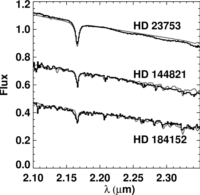
Figure 1: Spectra for three calibrators used to check the flux calibration procedure for KI (Section 2.2.2). The calibrated spectra are shown as black histograms. Nextgen spectra computed at the KI spectral resolution, using the source spectral types (see Table Constraining the Sub-AU-Scale Distribution of Hydrogen and Carbon Monoxide Gas around Young Stars with the Keck Interferometer), are shown as gray curves.

Instrumental scattered or thermal background light could add continuum emission to the KI data, leading to observed line-to-continuum ratios lower than intrinsic spectral features. To test for such effects, we compared observed and theoretical spectra for several of our main-sequence calibrator stars. Figure 1 demonstrates that the observed photospheric Br$\gamma$ absorption in these “check stars” is consistent with theoretical expectations, across a range of source colors and brightnesses (see Table Constraining the Sub-AU-Scale Distribution of Hydrogen and Carbon Monoxide Gas around Young Stars with the Keck Interferometer for spectral types and magnitudes). Thus the Br$\gamma$ spectra derived from the KI data do not seem to be affected substantially by instrumental scattering or background emission.

Since CO overtone emission occurs in the red end of the $K$-band, where thermal emission is stronger, uncorrected background emission may be more significant for CO than for the Br$\gamma$ region. Two of the check stars, HD 144841 and HD 184152, are expected to show some CO overtone absorption. The observed absorption features appear weaker than expected from the synthetic spectra (Figure 1). The largest discrepancy is seen for HD 184152, one of the faintest objects observed with KI. Uncorrected background emission would be relatively stronger for fainter objects, consistent with this observation. Thus, some caution is required when interpreting the CO overtone emission or absorption features in the KI spectra, particularly for fainter targets.

We measured squared visibilities ($V^{2}$) for our targets and calibrator stars in each of the 330 spectral channels across the $K$-band provided by the grism. The calibrator stars are main sequence stars, with known parallaxes, whose $K$ magnitudes are within 0.5 mags of the target $K$ magnitudes (Table Constraining the Sub-AU-Scale Distribution of Hydrogen and Carbon Monoxide Gas around Young Stars with the Keck Interferometer). We calculated the system visibility appropriate to each target scan by weighting the calibrator data by the internal scatter and the temporal and angular proximity to the target data (Boden et al. 1998). For comparison, we also computed the straight average of the $V^{2}$ for all calibrators used for a given source, and the system visibility for the calibrator observations closest in time. These methods all produce results consistent within the measurement uncertainties. We adopt the first method in our analysis.

Phases are measured in each spectral channel using the same “ABCD” procedure (Colavita 1999) used to determine $V^{2}$. These phases are then de-rotated so that the average phase of all channels is zero. Next, the phases versus wavelength are unwrapped to eliminate any jumps between -180^∘ and 180^∘. After computing weighted average differential phases for each target and calibrator scan, we determine a “system differential phase” using similar weighting employed above to calculate the system visibility.

The system differential phase is subtracted from the target differential phase. Since targets and calibrators are observed at similar airmasses, this calibration procedure removes most atmospheric and instrumental refraction effects. Finally, we remove any residual slope in the differential phase spectrum, since we can not distinguish instrumental slopes from those intrinsic to the target signal (e.g., Woillez et al. 2012). Since we are focused on small spectral regions around individual spectral features, we are largely insensitive to errors in these calibrations.

The measured fluxes, $V^{2}$, and differential phases contain contributions from the circumstellar material and from the central stars. To remove the central star, we first estimate its flux in each observed spectral channel using stellar parameters from the literature (see Table Constraining the Sub-AU-Scale Distribution of Hydrogen and Carbon Monoxide Gas around Young Stars with the Keck Interferometer) and a suitable Nextgen synthetic spectrum. The synthetic spectra are subtracted from the observed KI spectra to produce circumstellar fluxes for each spectral channel.

Circumstellar fluxes ($F_{\rm circ}$), visibilities ($V_{\rm circ}$), and differential phases ($\Delta\phi_{\rm circ}$) are given by the following equations (e.g., Eisner et al. 2010):

$$F_{\rm circ}=F_{\rm meas}-F_{\ast},$$ (1)

$$\Delta\phi_{\rm circ}=\tan^{-1}\left[\frac{V_{\rm meas}\sin(\Delta\phi_{\rm meas})(F_{\ast}+F_{\rm circ})}{V_{\rm meas}\cos(\Delta\phi_{\rm meas})(F_{\ast}+F_{\rm circ})-F_{\ast}}\right],$$ (2)

$$V_{\rm circ}=V_{\rm meas}\frac{\sin(\Delta\phi_{\rm meas})}{\sin(\Delta\phi_{\rm circ})}\left(\frac{F_{\ast}+F_{\rm circ}}{F_{\rm circ}}\right).$$ (3)

These equations imply that even if a spectral feature is not apparent in the observed spectrum, its presence may be implied in the circumstellar emission. For example, late-type stars have photospheric CO overtone absorption. If no absorption is seen in the observed spectra of such objects, this implies that the photospheric absorption is filled in by circumstellar emission.

One potential pitfall with this procedure is that the Nextgen templates only cover stars up to 10,000 K, while the Herbig Be stars in our sample (V1685 Cyg, AS 442, and MWC 1080) have higher effective temperatures. Such hot stars typically have shallower Br$\gamma$ absorption than cooler A stars, since the H ionization fraction in the stellar photosphere is higher. Thus the circumstellar Br$\gamma$ spectra for these objects may underestimate the true line-to-continuum ratios.

2.3 NIRSPEC Data

For four of our sample objects, VV Ser, AS 353 A, V1685 Cyg, and AS 442, we obtained NIRSPEC data on 2011 September 15. We used the high-dispersion mode with the 3 pixel slit, which provides a resolving power of $R\approx 24,000$. The NIRSPEC-7 filter was used with an echelle position of 62.25 and a cross-disperser position of 35.45. This provided seven spectral orders covering portions of the wavelength range between 1.99 and 2.39 $\mu$m. Included in these orders are the Br$\gamma$ line and the $v=2\rightarrow 0$ and $v=4\rightarrow 2$ CO bandheads.

Spectra were calibrated and extracted using the REDSPEC package (e.g., McLean et al. 2003). Reduction included mapping of spatial distortions, spectral extraction, wavelength calibration, heliocentric radial velocity corrections, bias correction, flat fielding, and sky subtraction. We divided our target spectra by the observed spectrum of HD 201320, an A0V star. We interpolated the A0V spectrum over the broad Br$\gamma$ absorption feature. Finally we multiplied the divided spectra by an appropriate blackbody template to calibrate the bandpass of the instrument. We did not attempt to flux calibrate the spectra, but instead applied scaling factors so that the NIRSPEC data had the same mean flux level (in a given spectral region) as the KI spectra.

3 Basic Results and Analysis

In this section we present the calibrated KI and NIRSPEC data, and discuss physical implications for the distribution of gaseous emission around our sample objects. We begin by comparing the KI spectra with our NIRSPEC observations (where available) and previous data from the literature. We then use the observed $V^{2}$ and $\Delta\phi$ for our sample to derive estimates of the spatial distributions and centroid positions of the emission as a function of wavelength. As we discuss below, Br$\gamma$ emission is prevalent from the sample, while CO overtone emission is relatively rare. We therefore present the results for the Br$\gamma$ and CO spectral regions separately in Sections 3.1 and 3.2.

3.1 Spectra and Spatial Distributions of Br $\gamma$ Emission

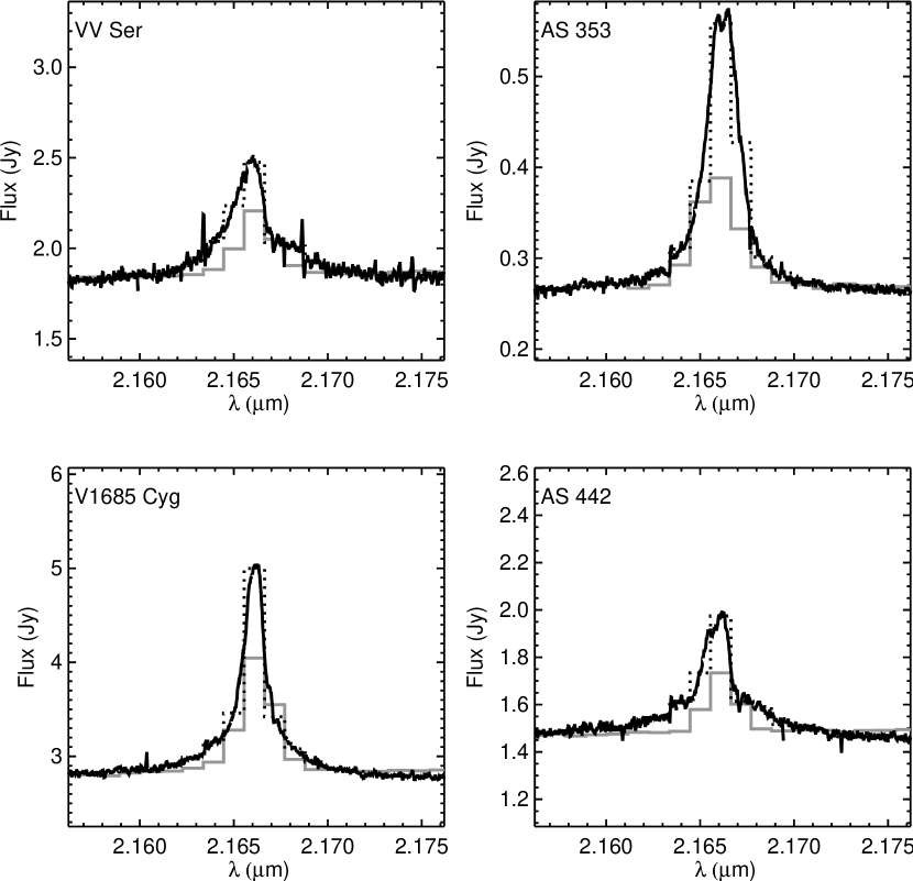
Figure 3: Spectra of Br$\gamma$ emission for four of our sample objects obtained with NIRSPEC (black curves). We also plot the KI spectra as gray histograms, and the NIRSPEC data smoothed to the KI spectral resolution as dotted black hitograms.

Calibrated spectra from KI, observed and with the stellar components subtracted (Equation 1), are shown for the Br$\gamma$ spectral region in Figure 2. Calibrated and scaled NIRSPEC spectra are plotted in Figure 3. While the NIRSPEC data have approximately 10 times higher spectral resolution than the KI data, the spatial resolution of the seeing-limited NIRSPEC observations is $\sim 1000$ times coarser.

The NIRSPEC data show higher line-to-continuum ratios for the Br$\gamma$ emission than do the KI data (Figure 3). Previous near-IR spectroscopy (Folha & Emerson 2001), with a spectral dispersion similar to the NIRSPEC data presented here, also found line-to-continuum ratios of the Br$\gamma$ emission higher than seen in our KI data. The lower line-to-continuum ratios in the KI data are due, in part, to the lower spectral dispersion. With $>10$ times higher dispersion, the NIRSPEC data suffer less dilution of strong spectral features. However the Br$\gamma$ lines are well-resolved, and dilution is only a minor effect (Figure 3).

The different fields of view of the two instruments may also play a role, with the larger field of view of NIRSPEC potentially sensitive to spatially extended Br$\gamma$ emission outside of the 50 mas field of view of KI. Br$\gamma$ emission is seen on $\gtrsim 1^{\prime\prime}$ scales in some young stars, comprising up to 10% of the total Br$\gamma$ flux (e.g., Beck et al. 2010). Extrapolating this finding to scales between 50 mas and $1^{\prime\prime}$ may explain the difference between the KI and NIRSPEC spectra. We explore this issue quantitatively in Section 4.

From the KI spectra, we compute the equivalent width of the Br$\gamma$ line for each source. Following Eisner et al. (2007c), we use these equivalent widths in conjunction with literature photometry and extinction estimates to determine the Br$\gamma$ line luminosities. These line luminosities are then converted into accretion luminosities using empirically-determined relationships for stars with masses $<1$ M_⊙ (Muzerolle et al. 1998) and $>1$ M_⊙ (Mendigutía et al. 2011). These relationships have not been calibrated beyond 6 M_⊙, and may not hold for the most massive Herbig Be stars in our sample, V1685 Cyg and MWC 1080. Equivalent widths, Br$\gamma$ line luminosities, and accretion luminosities for our sample are listed in Table 3.

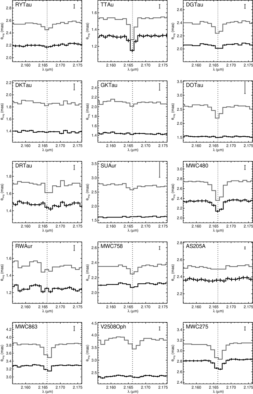
Figure 4: Uniform ring angular diameters of our sample, plotted in the spectral region around Br$\gamma$. Angular sizes computed directly from the observed $V^{2}$ are plotted with black histograms. Angular sizes of only the circumstellar emission, determined using Equation 3, are shown with gray histograms.

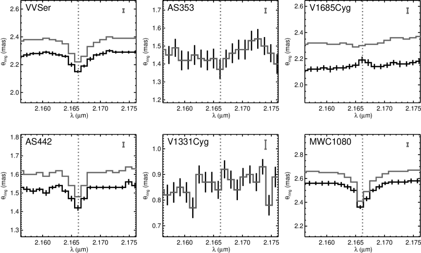
Figure 4: continued.

In addition to spectra, we measured squared visibilities for our targets, which constrain the relative spatial distributions of continuum and line emission components. We fit the $V^{2}$ data for each source, in each channel, with a simple uniform ring model (e.g., Eisner et al. 2004) to produce a “spectral size distribution” of the emission. The spectral size distributions based on the observed data, and for the circumstellar emission components (Equation 3), are shown in Figure 4.

For the majority of the observed targets, we infer a distinct spatial distribution for Br$\gamma$ emission and continuum emission (Figure 4). To quantify the relative distributions, we separate the complex visibility components due to the Br$\gamma$ line and the continuum, and fit each with uniform ring models (as in Eisner et al. 2010). The estimated sizes for the two components are listed for our sample in Table 4.

The Br$\gamma$ emission is generally found in a significantly more compact distribution. However for AS 353 A, V1685 Cyg, and V1331 Cyg, the inferred sizes for the line and continuum emission components are comparable. A few other objects (including DG Tau and DO Tau) show Br$\gamma$ emission sizes that are a significant fraction of the continuum emission sizes.

Differential phase signatures in the KI data indicate centroid offsets of various line emission components. We convert the measured $\Delta\phi$ values into centroid offsets as follows:

$$\Delta\theta=\Delta\phi\frac{\lambda}{2\pi B},$$ (4)

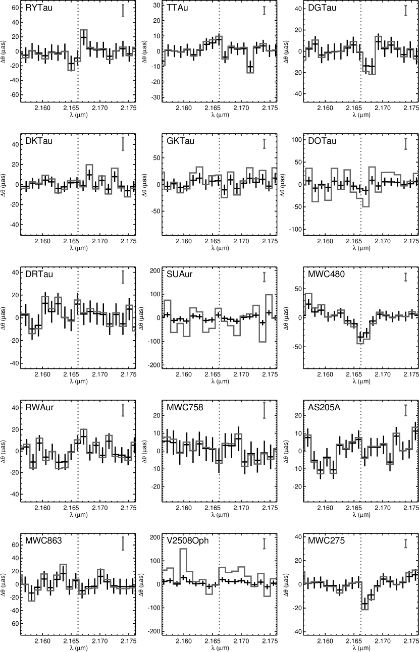
Figure 5: Centroid offsets of our sample, plotted in the spectral region around Br$\gamma$. Black histograms show the offsets derived for the observed data, and gray histograms show the centroid offsets for the circumstellar component of the emission, determined using Equation 2.

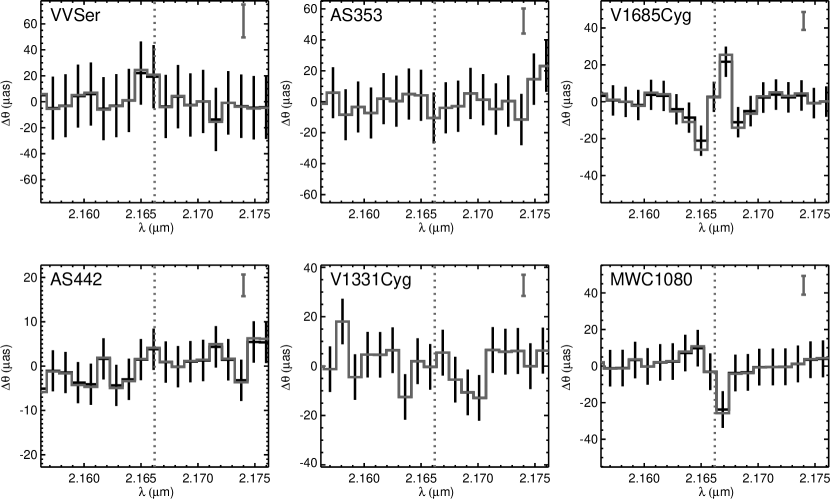
Figure 5: continued.

where $\lambda$ is the observed wavelength and $B$ is the projected baseline length. We also compute the centroid offsets for the circumstellar emission components (Equation 2). Centroid offsets are plotted in Figure 5 for the Br$\gamma$ order.

A number of targets show evidence for position offsets of different velocity components across the spectrally-resolved Br$\gamma$ line (Figure 5). For example, in RY Tau the red- and blue-shifted components of the emission have opposite (and approximately equal) position offsets. Such a signature resembles expectations for a spatially resolved Keplerian disk of emission. In contrast, MWC 275 shows a significant positional offset of only the red-shifted emission component, perhaps arguing for a bipolar infall where one lobe is (partially) obscured from view. We model these signatures quantitatively below in Section 4.

3.2 Spectra and Spatial Distributions of CO Overtone Emission

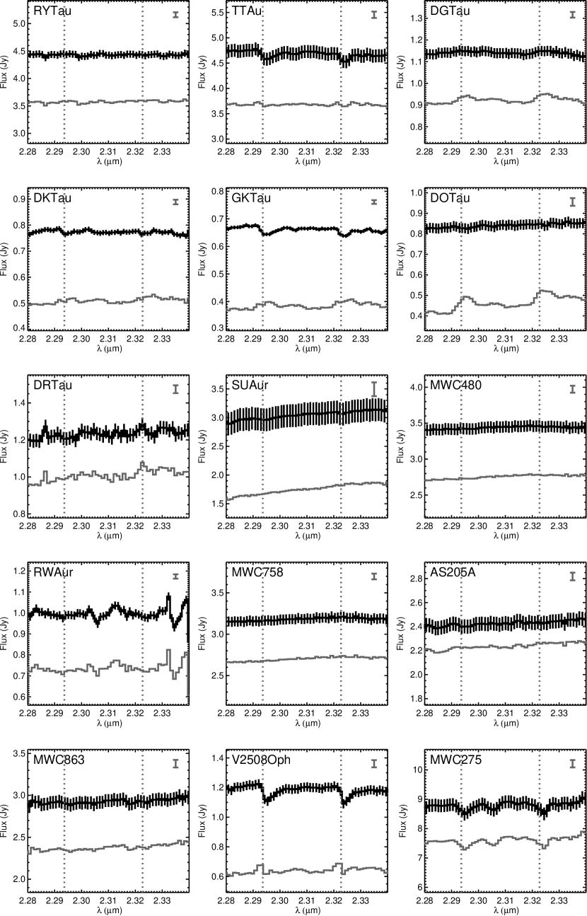
Figure 6: Flux versus wavelength for our sample objects measured with KI. This figure focuses on the spectral region around the CO rovibrational overtone transitions. The solid histogram shows the observed spectrum for the target, and the gray histogram shows the flux of the circumstellar component only. For clarity of presentation, we have not plotted the error bars associated with the circumstellar fluxes; the magnitudes of the uncertainties are indicated in the upper right corners. Dotted gray lines indicate the central (rest) wavelengths of the $v=2\rightarrow 0$ bandhead at 2.2936 $\mu$m and the $v=3\rightarrow 1$ bandhead at 2.3227 $\mu$m.

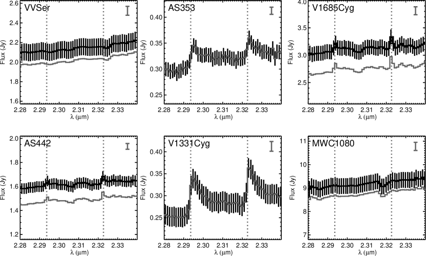
Figure 6: continued.

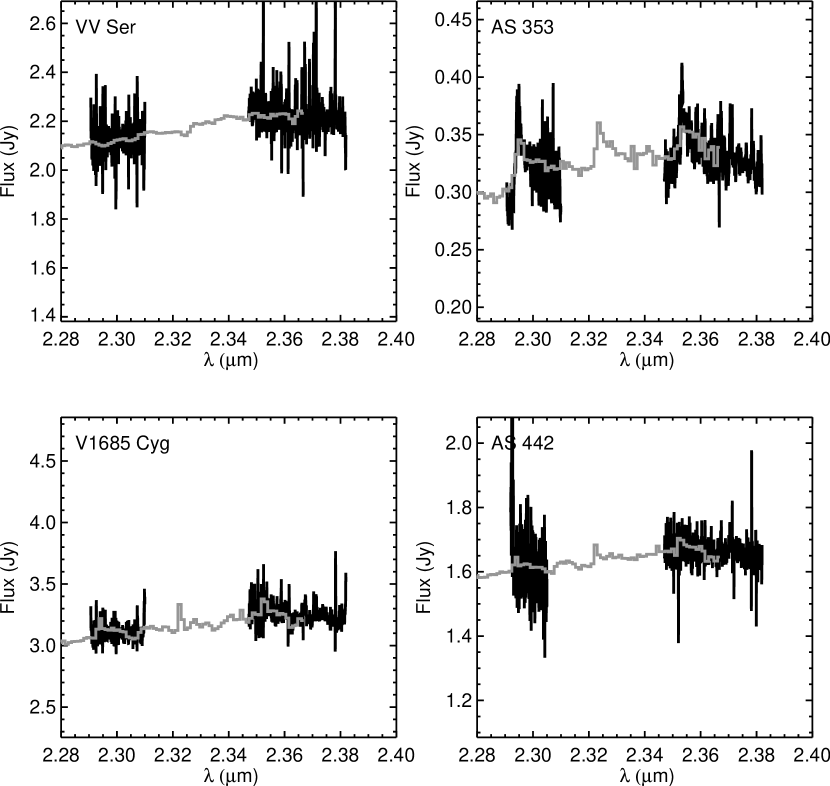
Figure 7: Spectra of CO overtone emission from four of our sample objects obtained with NIRSPEC (black curves). These spectra, obtained in two separate orders, cover the $v=2\rightarrow 0$ and $v=4\rightarrow 2$ bandheads. We also plot the KI spectra as gray histograms.

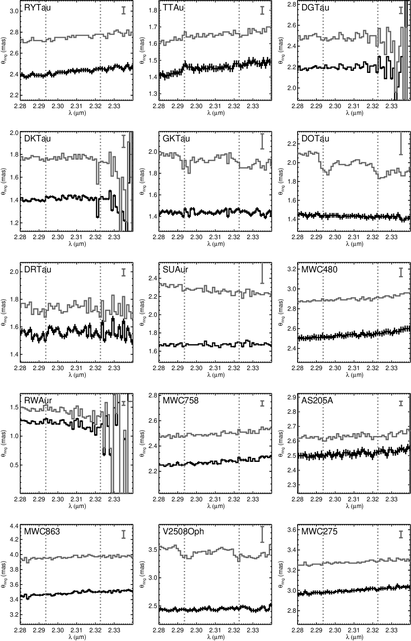
Figure 8: Uniform ring angular diameters of our sample, plotted in the spectral region around the CO overtone bandheads. Angular sizes computed directly from the observed $V^{2}$ are plotted with black histograms. Angular sizes of only the circumstellar emission, determined using Equation 3, are shown with gray histograms.

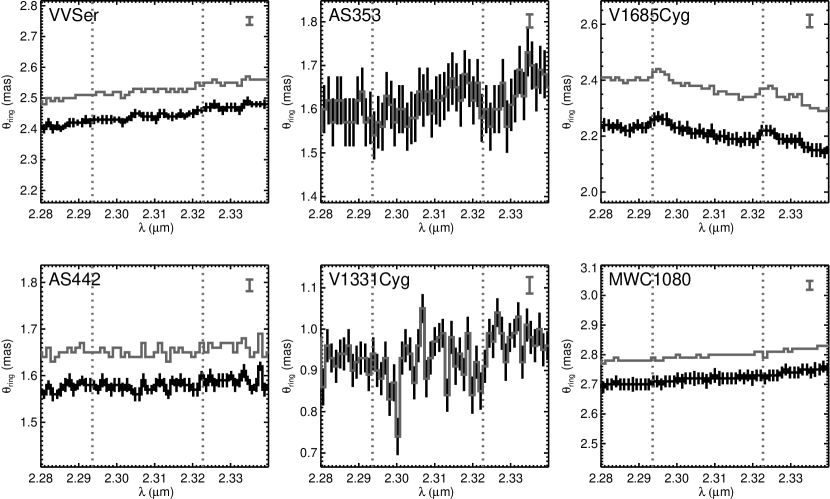
Figure 8: continued.

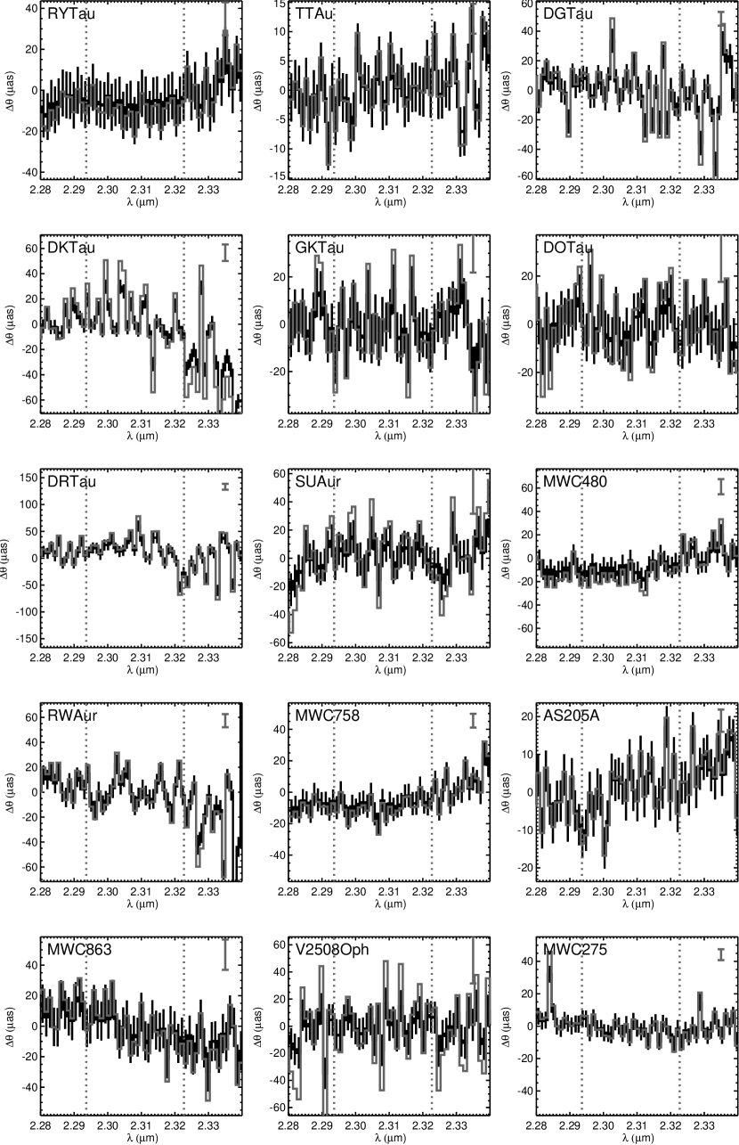
Figure 9: Centroid offsets of our sample, plotted in the spectral region around the CO overtone bandheads. Black histograms show the offsets derived for the observed data, and gray histograms show the centroid offsets for the circumstellar component of the emission, determined using Equation 2.

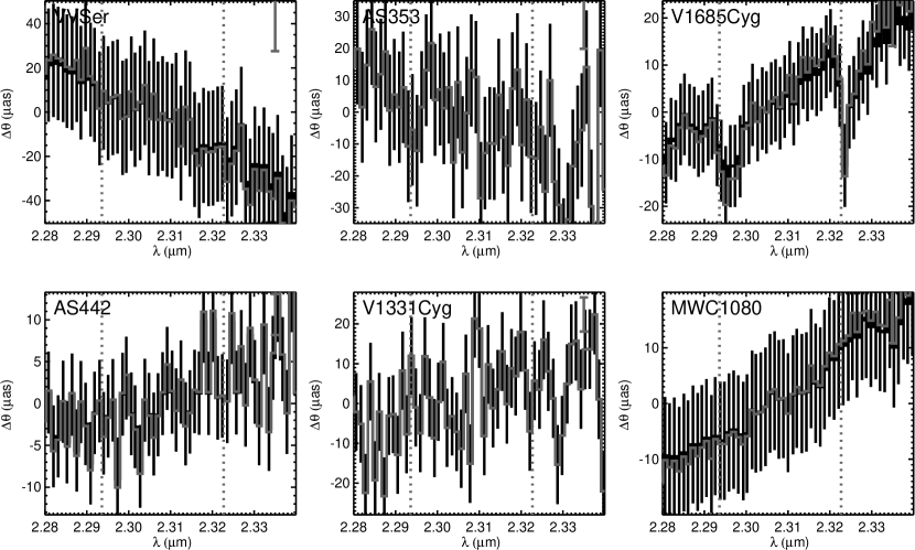
Figure 9: continued.

KI and NIRSPEC spectra of our sample, covering the spectral region including the CO overtone bandheads, are shown in Figures 6 and 7. Spectral size distributions, and centroid offsets across the CO bandheads, are shown in Figures 8 and 9, respectively.

Of the 21 objects in our sample, only two—AS 353 A and V1331 Cyg—show strong CO overtone emission. CO emission has been observed previously for both of these (e.g., Carr 1989; Biscaya et al. 1997; Prato et al. 2003). The line-to-continuum ratio observed here for V1331 Cyg is comparable to that seen in previous observations, including ones with similar resolution to the KI data (Biscaya et al. 1997; Eisner et al. 2013). The line-to-continuum ratio of AS 353 A in our KI and NIRSPEC data is somewhat higher than seen in previous observations (Carr 1989; Prato et al. 2003), although there does seem to be some variability in the CO emission strength (Biscaya et al. 1997).

In addition to AS 353 A and V1331 Cyg, a number of targets show tentative evidence of CO overtone emission (Figure 6). DG Tau and DO Tau both exhibit circumstellar CO emission features, although such features are absent in the calibrated (star+circumstellar) spectra. There are also hints of circumstellar CO emission in DK Tau A and GK Tau, although the calibrated spectra show CO absorption. Thus, any inferred CO emission in these objects depends on the accuracy of the removal of stellar CO absorption.

In Section 2.2.2 we suggested that CO overtone absorption features in faint objects might appear weaker in observed spectra than their intrinsic values, perhaps because of uncorrected thermal background emission. DG Tau, DK Tau A, GK Tau, and DO Tau are all among the faintest objects in the sample, where uncorrected background emission would have a larger effect. The small apparent CO emission in DK Tau A and GK Tau is likely an artifact of the calibration process. However, DG Tau is known to show CO overtone emission (e.g., Carr 1989), and the signal in DO Tau is fairly large.

Given that AS 353 A and V1331 Cyg exhibit CO emission at levels similar to (or higher than) previous observations, it seems improbable that the CO features in DO Tau (which is similarly faint to those targets) could be completely spurious. However, any line enhancement arising from instrumental errors will affect the data strongly for DO Tau, because the ratio of stellar to circumstellar flux is high (see Equations 1–3). As seen in Figure 6, the stellar component is approximately the same brightness as the circumstellar component in the CO spectral region. In contrast, errors for DG Tau will be less severe, since its stellar flux is only a small fraction of its circumstellar flux (Figure 6).

V1685 Cyg and AS 442 also show weak CO emission features, while MWC 275 shows apparent CO overtone absorption in its circumstellar spectrum (Figure 6). These are hot stars, and these tentative detections do not rely on accurate subtraction of the stellar photospheric spectra. However calibration artifacts (e.g., due to mismatches between observed and template spectra for late-type calibrators) may be responsible for the apparent features. Recent CO overtone spectra of these sources show no features in AS 442 or MWC 275, but possible evidence for weak CO emission in V1685 Cyg (Eisner et al. 2013). Strong features seen in the $V^{2}$ and differential phase data for V1685 Cyg (Figures 8 and 9) strengthen the case for real CO emission in this source. We therefore discount the apparent CO features in MWC 275 and AS 442, but include V1685 Cyg in our further analysis of the CO spectral region.

For our analysis we select those objects with the most significant detections of CO emission features. This sub-sample includes DG Tau, DO Tau, AS 353 A, V1685 Cyg, and V1331 Cyg. Since the CO detections for DG Tau and DO Tau depend on the removal of the stellar photospheric spectrum, these should be treated with some caution. The detection rate in our sample, 5/21, is similar to the detection rate in previous surveys for CO overtone emission (e.g., 9/40 in Carr 1989).

For this sub-sample of CO overtone emitters, we estimate the spectral size distribution in the CO region. The continuum sizes in the CO region (Table 5) may differ from those in the Br$\gamma$ region (Table 4). Small, monotonic, changes with wavelength are expected (for all targets) if continuum emission arises in extended distributions of circumstellar matter exhibiting temperature gradients. These broadband slopes were modeled for many of our targets in previous work (e.g., Eisner et al. 2007a, 2009). However the observed $V^{2}$ for V1685 Cyg show unusually large changes with wavelength, including a non-monotonic dependence. We illustrate this behavior in Figure 10, comparing V1685 Cyg to AS 442, the latter representative of the spectral $V^{2}$ behavior across the sample. We do not have a clear explanation for the $V^{2}$ observed from V1685 Cyg, but suggest below that binarity may help to explain the peculiar continuum shape.

Separating the continuum and line emission components, we determine approximate spatial locations of the first two CO overtone bandheads (Table 5). For AS 353 A and V1331 Cyg, the inferred sizes of the emission arising in the first two overtone bandheads are comparable to the continuum sizes. For V1685 Cyg the CO emission appears more widely distributed than the continuum emission, although the estimated sizes of CO-emitting regions have large uncertainties. In contrast, the CO emission in DG Tau and DO Tau appears more compactly distributed than the continuum emission.

The centroid offsets determined for the CO spectral region are noisy (Figure 9), and it is difficult to discern clear signatures at the wavelengths of the CO overtone bandheads. However one target, V1685 Cyg, does appear to have emission from the CO bandheads that is spatially offset from the continuum emission.

4 Kinematic Modeling

Following Eisner et al. (2010) we model our KI data with both disk and infall/outflow models. The properties of these models are similar to Eisner et al. (2010), although we explore a substantially larger range of parameter values here. We describe the models below, and refer to Eisner et al. (2010) for details of how each model parameter affects synthetic data. We will use the same models developed for the KI data to interpret the NIRSPEC spectra.

The disk and outflow models are both fitted to the KI Br$\gamma$ data. The KI data in the CO spectral region are typically noisier than in the Br$\gamma$ region, making it difficult to constrain models well. We will therefore pursue a less rigorous modeling effort in this spectral region, restricting our attention to disk models, and comparing to data rather than performing rigorous fits.

As in Eisner et al. (2010) we make the simple assumption that continuum emission is confined to a ring whose annular width is 20% of its inner radius. This assumption is consistent with models where continuum emission traces dust near the sublimation radius (e.g., Dullemond et al. 2001; Eisner et al. 2004; Isella & Natta 2005). The size of the continuum ring is determined from a fit of a uniform ring model to $V^{2}$ data in spectral regions adjacent to those where Br$\gamma$ or CO emission is observed (Tables 4 and 5). We determine the ring radius, $R_{\rm ring}$, for all position angles and inclinations considered for our gaseous disk models. The temperature of the ring is set so that the continuum flux level matches the observed continuum fluxes. Neither $R_{\rm ring}$ nor $T_{\rm ring}$ are free parameters in the models discussed below.

4.1 Keplerian Disk Models

We assume that while the continuum emission is confined to a ring, the gaseous emission resides in a disk extending from $R_{\rm in}$ to $R_{\rm out}$. Both the disk and the ring of continuum emission have a common inclination, $i$, and position angle, $PA$, that are free parameters.

The brightness profile of the gaseous disk is parameterized with a power-law,

$$B_{\rm disk}(R)=B_{\rm in}\left(\frac{R}{R_{\rm in}}\right)^{-\alpha}.$$ (5)

The value of $\alpha$ depends on the temperature profile and surface density profile of the disk. For optically thin gas following a surface density profile similar to the minimum mass solar nebula (Weidenschilling 1977), and heated by thermal radiation from the central star, $\alpha\approx 2$. However the temperature and surface density profiles are not well-constrained, and so we leave $\alpha$ as a free parameter in our modeling. Instead of using $B_{\rm in}$, we normalize the brightness profile so that the resulting spectrum has a specified line-to-continuum ratio, $L/C$. $L/C$ is defined as the ratio of the total flux of the gaseous emission, integrated over space and velocity, to the continuum flux level.

We assume the gas to be in Keplerian rotation, with a radial velocity profile,

$$v_{\rm obs}(R)=\sqrt{\frac{GM_{\ast}}{R}}\cos(\theta)\sin(i).$$ (6)

Here, $M_{\ast}$ is the stellar mass, $\theta$ is the azimuthal angle in the disk for a given $(x,y)$ in cartesian coordinates, and $i$ is the disk inclination. For simplicity, we do not enter exact values of $M_{\ast}$ for each source into the model (these are not determined to high accuracy for most objects). Rather, we assume a stellar mass of 1 M_⊙ for the T Tauri stars in our sample, 3 M_⊙ for the Herbig Ae stars, and 10 M_⊙ for the Herbig Be stars V1685 Cyg and MWC 1080.

To minimize the number of free parameters in our model grid we set $R_{\rm out}=R_{\rm ring}$. Thus we assume that any gaseous emission that may exist at stellocentric radii larger than $R_{\rm ring}$ is hidden by the optically thick dust disk. This may not be an accurate assumption, especially for CO emission where models suggest excitation in disk surface layers is possible (e.g., Glassgold et al. 2004; Gorti & Hollenbach 2008). We therefore relax this assumption when modeling the CO emission (Section 4.4).

We explore the following values of free parameters in our grid of Keplerian disk models: $R_{\rm in}=0.01,0.02,0.03,0.04,$ and 0.05 AU; position angle = $0,25,50,75,$ and 90^∘; inclination = $5,25,50,$ and $75^{\circ}$; $L/C=0.1,0.25,0.5,0.75,$ and 1.0; and $\alpha=2,3,$ and 4. Our grid contains 1500 models, compared to the 243 disk models computed in Eisner et al. (2010).

4.2 Infall/Outflow Models

We construct models consisting of a face-on ring of continuum emission (described above) and a bipolar conical gas infall/outflow. We assume an infall/outflow cone with an opening angle of $5^{\circ}$, a position angle, $PA$, and an inclination with respect to the plane of the sky, $\phi$. We allow the infall/outflow to extend from an outer radius, $R_{\rm out}$ to an inner radius, $R_{\rm in}$. In contrast to the disk model considered above, $R_{\rm out}\neq R_{\rm ring}$ here.

The velocity of material in this cone is described as a radial power-law:

$$v_{\rm obs}(R)=v_{\rm in}\left(\frac{R}{R_{\rm in}}\right)^{-\beta}\sin\phi.$$ (7)

Here the velocity of material at the inner edge of the infall/outflow structure, $v_{\rm in}$, is chosen to produce a specified linewidth of the emission,

$$\Delta v=v_{\rm in}\sin\phi.$$ (8)

Examination of Equations 7 and 8 shows that the velocity profile depends on $\Delta v$, $R_{\rm in}$, and $\beta$, but not directly on $\phi$. The geometry of the outflow of the sky depends on $PA$, as well as on $R_{\rm in}$ and $R_{\rm out}$, but again not explicitly on $\phi$. We thus fix $\phi=45^{\circ}$ in our models.

We include another cone, reflected through the origin, with the same velocity profile multiplied by $-1$. The brightness distribution of the infall/outflow cones is

$$B_{\rm infall/outflow}(R)=B_{\rm in}\left(\frac{R}{R_{\rm in}}\right)^{-\alpha},$$ (9)

where $B_{\rm in}$ is chosen to reproduce a specified line-to-continuum ratio. As above, $L/C$ is defined as the total, integrated flux of the gaseous emission over the continuum flux. $\alpha$ combines the temperature and surface density profile of the infall/outflow structure into a single parameter. Finally, we include as a free parameter a factor by which the flux in one of the two cones or “poles” or the infall/outflow may be scaled. We denote this factor as $f_{\rm a}$, since it represents an asymmetry in the model.

We explore the following values of free parameters in our grid of infall/outflow models: $R_{\rm in}=0.01,0.02,0.03,$ and 0.04, AU; $R_{\rm out}=0.05,0.1,0.5,$ and 1 AU; position angle = $0,20,40,60,$ and 80^∘; $\beta=1,2,$ and 3; $\Delta v=250,375,$ and 500 km s^-1; $L/C=0.1,0.5,$ and 1.0; $\alpha=2,3,$ and 4; and $f_{\rm a}=0.1,0.5,$ and 1.0. The computed grid includes 19440 infall/outflow models, compared to the 2916 models included in Eisner et al. (2010).

4.3 Results for the Br$\gamma$ Spectral Region

After computing synthetic fluxes, $V^{2}$, and $\Delta\phi$ values for grids of both disk and infall/outflow models, we compute the $\chi^{2}$ residuals between these and the observed quantities from KI. The total $\chi^{2}$ is given by

$$\chi^{2}_{\rm tot}=\sqrt{(\chi^{2}_{\rm flux})^{2}+(\chi^{2}_{\rm V^{2}})^{2}+(\chi^{2}_{\rm\Delta\phi})^{2}}.$$ (10)

Finally, we minimize $\chi^{2}_{\rm tot}$ to determine the “best-fit” model. Even though this grid of models samples significantly more parameter values than previous work, it remains sparsely sampled, and hence we can not give rigorous error intervals on the fitted parameters.

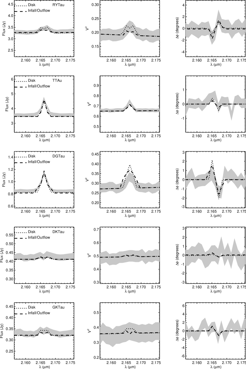
Figure 11: Synthetic data for best-fit disk and infall/outflow models (dotted and dashed curves) plotted atop the 1$\sigma$ region allowed by the observed data (gray shaded regions).

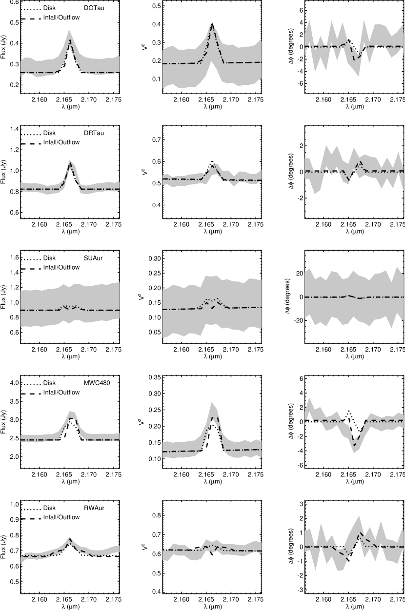
Figure 11: continued.

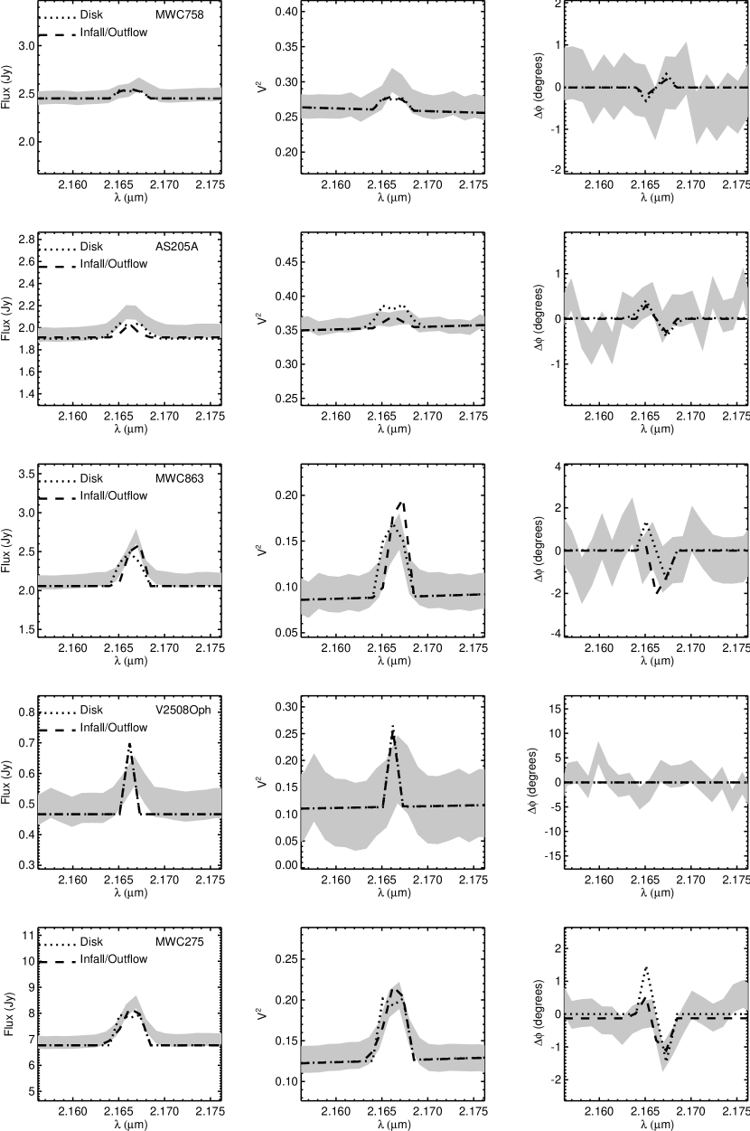
Figure 11: continued.

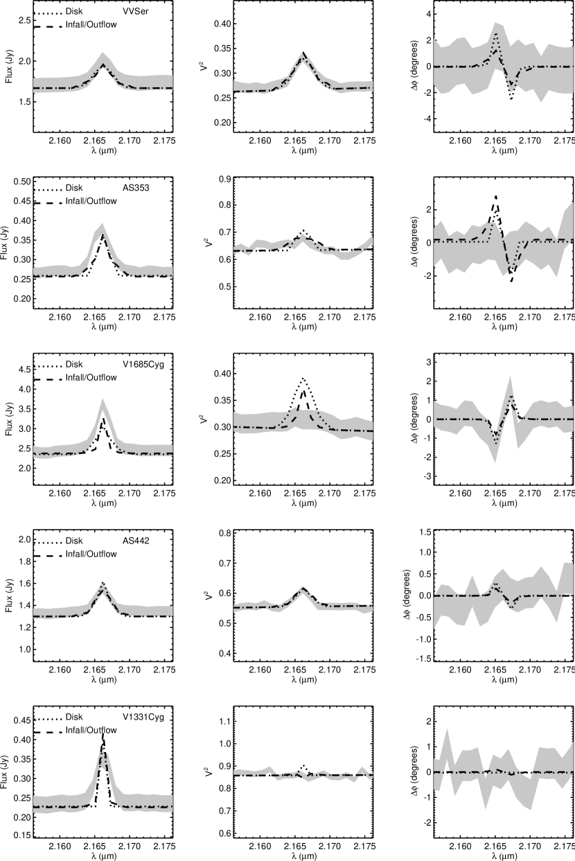
Figure 11: continued.

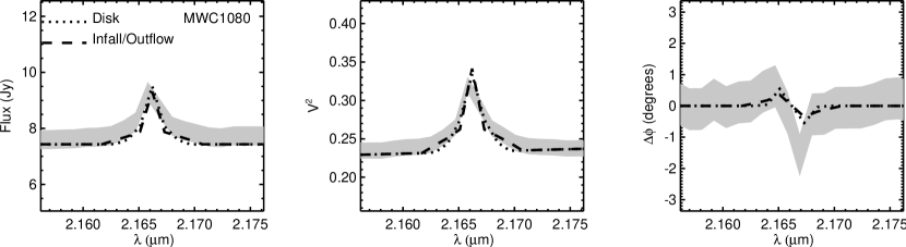
Figure 11: continued.

The best-fit models are illustrated in Figure 11. Reduced $\chi^{2}$ values, and parameters of the best-fitting models, are listed in Table 6. Disk models and infall/outflow models generally produce fits of comparable quality. This differs from the modeling in Eisner et al. (2010), and reflects the better fits of disk models that are achieved with the larger grid of models used here. However, we do confirm that for objects with the highest signal-to-noise data, infall/outflow models are generally preferred. This preference is based largely on the differential phase data, which can constrain asymmetric structures compatible with infall/outflow models but inconsistent with disk models. For the brighter sources in our sample the differential phase data have high enough signal-to-noise to discern such asymmetries.

For a handful of targets neither model provides a particularly good fit to the combined KI dataset. Formally the worst fits are obtained for RW Aur, V2508 Oph, AS 353 A, and V1685 Cyg (Table 6), although the $\chi_{\rm r}^{2}$ values are all smaller than unity, suggesting that none of the fits are terrible. Examination of Figure 11 suggests that the fits for RW Aur, V2508 Oph, and AS 353 A may have higher $\chi_{\rm r}^{2}$ values simply because of somewhat higher scatter in the data. However V1685 Cyg is a bright source with high signal-to-noise, and the fits are clearly inconsistent with the observed $V^{2}$ data. The model places Br$\gamma$ emission on compact scales, while the lack of a clear $V^{2}$ signature suggests a similar spatial distribution of line and continuum emission. The best-fit model selected the largest values of $R_{\rm in}$ and $R_{\rm out}$ available, 0.04 AU and 1 AU, respectively. For comparison, the continuum size is 1.17 AU (Table 4). A better fit to the data would likely be achieved with a Br$\gamma$ distribution centered closer to the continuum emission region.

We noted above that the Br$\gamma$ spectra measured with NIRSPEC have higher line-to-continuum ratios than the KI spectra. For this reason we did not attempt to model the NIRSPEC data at the same time as the KI dataset. We will now attempt to reconcile the best-fit models, determined for the KI data, with the NIRSPEC spectra.

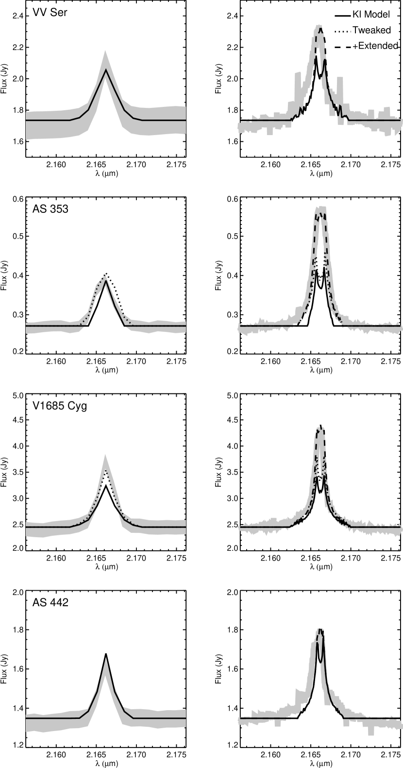
Figure 12: Observed and synthetic Br$\gamma$ spectra for targets observed by NIRSPEC. Left panels show KI spectra and right panels show NIRSPEC spectra (gray regions). Solid curves are the predicted spectra for the best-fit model determined from the KI dataset. In some cases, we made minor tweaks to this model to better fit the NIRSPEC data, without materially affecting the quality of the fits to the KI data (dotted curves). In all cases, the best-fit models do not fit the NIRSPEC data well. To improve the fits, for each source we add a Gaussian with FWHM between 25 and 75 km s^-1. This range of FWHM corresponds to Keplerian velocities at stellocentric radii of a few AU for our targets. The Gaussian component thus represents extended emission that might be outside of the KI FOV, but well within the NIRSPEC FOV.

First, we compute the expected Br$\gamma$ spectra for our best-fit models at the spectral resolution of the NIRSPEC data. Given the similar quality of the disk and outflow model fits for these objects (Table 6), we adopt the disk models for computational expediency. We adjusted $L/C$ to maintain a constant line flux between the KI and NIRSPEC data, but left all other model parameters unchanged. Synthetic NIRSPEC spectra for the best-fit disk models are shown as solid curves in Figure 12.

For AS 353 A and V1685 Cyg, the best-fit model did not fit the KI spectra perfectly (owing to limited model grid sampling), and so we tweaked the model to yield superior fits to the NIRSPEC data without altering the fit quality to the KI data. For AS 353 A we changed $R_{\rm in}$ from 0.01 to 0.003 AU, and for V1685 Cyg we increased $L/C$ by $\sim 30\%$. These “tweaked” models are shown with dotted lines in Figure 12.

As expected, synthetic spectra from our best-fit models, after minor tweaking where appropriate, under-predict the Br$\gamma$ lines seen in NIRSPEC data. We speculated above that NIRSPEC may be sensitive to spatially extended Br$\gamma$ emission on scales beyond the sensitivity of KI. The relevant spatial scales would be beyond a few AU, which would correspond to Keplerian velocities of $\sim 50$ km s^-1 for these objects. We added Gaussians with FWHM between 25 and 75 km s^-1 to the synthetic spectra, to simulate the addition of an extended emission component. The dashed curves in Figure 12 show that adding these low-velocity, possibly spatially extended emission components, can indeed produce resultant spectra similar to the observed NIRSPEC spectra.

It is interesting to note that the NIRSPEC data are sensitive not only to larger spatial scales, but also potentially to smaller spatial scales than the KI data. The higher dispersion of NIRSPEC means that more extreme velocities–which likely trace matter at the smallest stellocentric radii–can be constrained. The tweaked model for AS 353 A is a case-in-point, where the NIRSPEC data compel us to consider a model extending to higher velocities and smaller spatial scales.

Figure 12 shows that the best-fit disk models produce double-peaked line profiles at the spectral resolution of the NIRSPEC data. With the addition of spatially extended emission, the central dip in the line profiles is filled in, and the observed NIRSPEC data can be reproduced. If our explanation of the discrepancy between NIRSPEC and KI spectra as the result of extended emission is incorrect, then disk models would be ruled out. As discussed in Eisner et al. (2010), infall/outflow models can produce narrower line profiles while still reproducing the KI $V^{2}$ and differential phase data. However infall/outflow models would still struggle to simultaneously reproduce the NIRSPEC and KI data (which are not consistent with each other), precluding a simple alternative explanation.

4.4 Modeling Results for the CO Spectral Region

Given the relatively poor quality of the KI data in the CO spectral region, we do not attempt a rigorous $\chi^{2}$ minimization over our model grid. Instead we assume that the CO emission traces Keplerian disks in our targets (as suggested by previous line profile modeling; e.g., Najita et al. 1996a), and perform a by-eye minimization over varied model parameters. We do not consider infall/outflow models for the CO data. We perform this analysis for the sub-sample of objects with detected CO overtone emission, listed in Table 5.

For each source we use as a starting point the best-fit disk model determined for the Br$\gamma$ spectral region (Table 6). For the Br$\gamma$ modeling, we described the radial brightness distribution with a singe parameter, $\alpha$. This is appropriate, since the Br$\gamma$ emission arises from a single transition, and so there is no explicit dependence of the synthetic spectrum on temperature (although the transition requires population of the $n=7$ state of hydrogen, which implies a gas temperature $\gtrsim 10,000$ K).

In contrast, the CO bandheads are made up of multiple transitions, and the synthetic spectrum depends explicitly on temperature. We therefore replace $\alpha$ with exponents on power-law profiles of gas temperature and surface density. We assume that the temperature power law has an exponent of $-0.5$, similar to values used in previous modeling of CO overtone emission (e.g., $\sim-0.4--0.75$ used by Najita et al. 1996a; Carr et al. 2004). We take the surface density power law exponent to be $-1.5$, as calculated for the protosolar nebula (Weidenschilling 1977); this value is also consistent with previous modeling of spatially resolved observations of inner disk emission across a broad wavelength range (e.g., Kraus et al. 2008b). These profiles are used with CO line opacities from HITEMP (Rothman et al. 2005) to calculate the emergent spectrum as a function of disk radius.

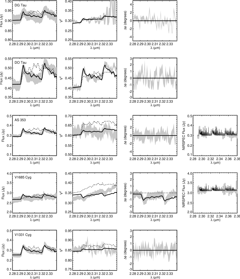
Figure 13: Synthetic spectra, $V^{2}$, and $\Delta\phi$, and computed for disk models, compared to KI data and NIRSPEC spectra (where available). Dotted curves show synthetic data for the best-fit models determined for the Br$\gamma$ emission, listed in Table 6. To better fit the data, we adjusted these models by varying $R_{\rm in}$ and $R_{\rm out}$ for all sources, and introducing a spatial offset between CO and continuum for V1685 Cyg (solid curves). As described in Section 4.4, these models confine CO emission to disk regions with fractional widths of 20% and temperatures $\gtrsim 3000$ K.

Synthetic spectra, $V^{2}$, and $\Delta\phi$ for these models are shown as dotted curves in Figure 13. These models do not match the data well. In all cases the models produce too much emission in between the first two overtone bandheads. The lines in this spectral region are relatively stronger in cooler CO gas, at temperatures $\lesssim 2,000$ K. Because our models assume a radial temperature gradient, they all include contributions from such cool gas at larger radii.

The synthetic data for the models generated from Table 6 are also discrepant from the $V^{2}$ data in most cases. For DO Tau, the model $V^{2}$ fall below the data, suggesting that the model CO emission is more extended than implied by the observations. For AS 353 A, V1685 Cyg, and V1331 Cyg, the opposite is true; models imply CO distributions more compact than the data. One target, V1685 Cyg, also shows centroid offsets that are not reproduced with this simple disk model.

To find models that reproduce the observations better, we allow $R_{\rm in}$ and $R_{\rm out}$ to vary. Given that cool CO emission is inconsistent with the data, we make the further assumption that $R_{\rm out}=1.2R_{\rm in}$; i.e., we restrict the CO emission to a narrow spatial and temperature distribution. Synthetic data from models with CO confined to such rings are shown as solid curves in Figure 13. These models provide superior fits to the data than the ones based entirely on the Br$\gamma$ emission geometry.

For all sources, our models produce CO emission at temperatures $\gtrsim 3000$ K; since the HITEMP opacities do not cover higher temperatures, we can not constrain $T$ more precisely. The inner radius of the CO emission in models for AS 353 A and V1331 Cyg are comparable to the continuum radii. For V1685 Cyg, the model places the CO emission at radii $\sim 30\%$ larger than the continuum emission. In contrast, the CO emission for DO Tau appears to be located at much smaller radii than the continuum: Figure 13 shows a model with CO located at $R_{\rm in}=0.01$ AU. Finally, for DG Tau, the CO emission is located interior to the continuum emission, although this is not well-constrained by the data. The ring model shown in Figure 13 represents CO at a radius of $\sim 0.1$ AU.

V1685 Cyg also shows a clear differential phase signature in the CO bandhead wavelengths. To model this, we introduce a spatial offset of $\sim 0.5$ mas ($\approx 0.5$ AU) between the centroid of the CO emission ring and the centroid of the continuum emission. Physically, such an offset seems difficult to explain with a model where gas and dust trace the same physical component. However if the CO traces a different source than the continuum, for example a binary companion at $\sim 0.5$ AU separation, then such a large offset could arise (see Section 5.4).

5 Discussion

5.1 Continuum Emission

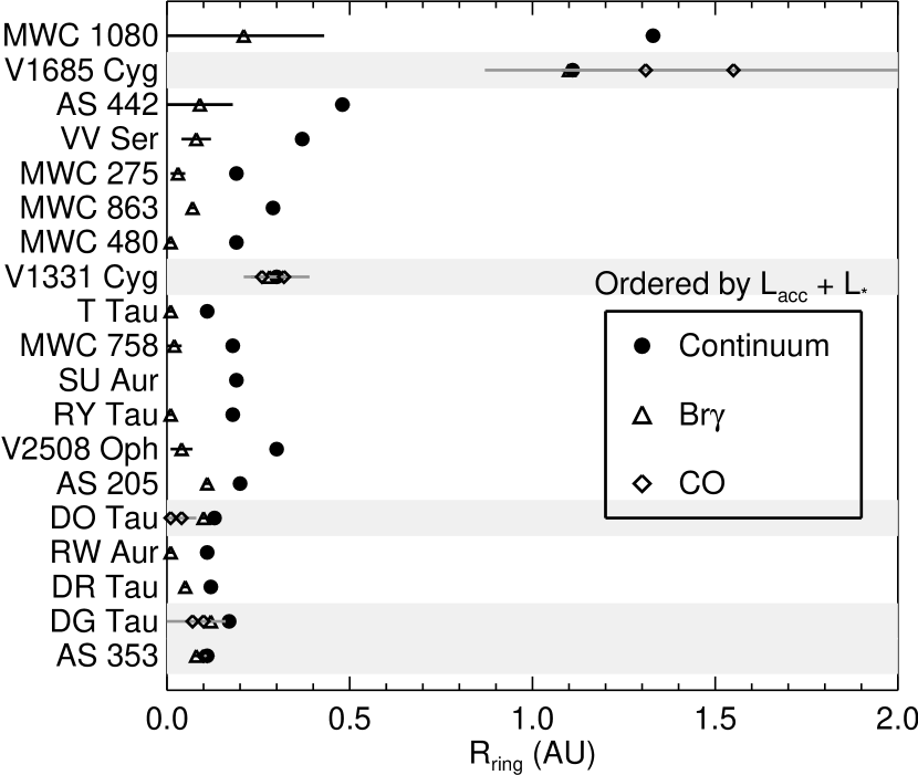
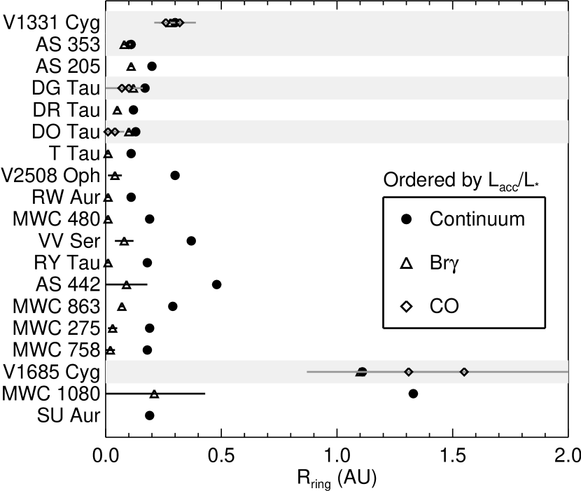
Figure 14: Spatial distributions of continuum, Br$\gamma$, and CO emission for our sample, based on fitted uniform ring radii (Tables 4 and 5). The error bars for the sizes of emission in the $v=2\rightarrow 0$ and $v=3\rightarrow 1$ CO bandheads are plotted as gray lines, while those of the continuum and Br$\gamma$ sizes are plotted as black lines. The error bars are often smaller than the symbol sizes. In the left panel, we plot objects in order of total luminosity (the sum of stellar and accretion luminosity). In the right panel, we order objects by $L_{\rm acc}/L_{\ast}$. We highlight the sub-sample of CO overtone emitters with light gray shading.

The inferred sizes of continuum emission regions for our sample are between $\sim 0.1$ and 1.3 AU (Table 4), compatible with previous measurements (e.g., Eisner et al. 2007b, 2009). In Figure 14, we plot the continuum sizes for each source, ordered by source luminosity. The luminosity is the sum of the stellar luminosity (from the literature) and the accretion luminosity listed in Table 3. The continuum size generally increases with source luminosity, and the relationship is consistent with an origin of the continuum emission in dust sublimation fronts (e.g., Monnier & Millan-Gabet 2002; Eisner et al. 2004; Monnier et al. 2005).

However the continuum may not trace dust only. Previous work suggested that the continuum emission from young stars—including many in our sample—contained contributions from matter hotter than dust sublimation temperatures, perhaps tracing free-free emission from H or H^- (e.g., Eisner et al. 2009). If some of the continuum emission is due to opacity from hot gas, measured continuum radii may lie between the compactly distributed hot gas and cooler dust at larger radii.

5.2 Br$\gamma$ Emission

Most objects in our sample show Br$\gamma$ emission with a compact distribution. Inferred sizes of the Br$\gamma$ emission are typically $\lesssim 0.05$ AU, considerably smaller than continuum sizes (Table 4). Kinematic modeling confirms that Br$\gamma$ emission extends in to such small stellocentric radii for nearly all targets (Table 6).

Magnetospheric accretion models predict that matter falling in along stellar magnetic field lines will glow brightly near to the stellar surface, where it converts most of its gravitational potential energy to radiation, and so we would expect to see Br$\gamma$ emission from very close to the stellar surface in this case (e.g., Muzerolle et al. 1998). For accretion via a Keplerian disk extending to the stellar surface, Br$\gamma$ emission would likely trace the shock at the disk/stellar surface boundary layer (e.g., Lynden-Bell & Pringle 1974). The compact Br$\gamma$ emission, and the asymmetric differential phases for some sources (Figure 5), suggest asymmetric Br$\gamma$ emission morphologies compatible with bipolar infall models. Asymmetric emission could arise from a tilted dipole accreting preferentially from one side of the disk, or from symmetric magnetospheric infall where one lobe is partially obscured by the disk.

Further support for magnetospheric accretion columns as the origin of the Br$\gamma$ emission comes from analysis of line profiles observed at higher spectral (but lower spatial) resolution. While most of our targets exhibit H$\alpha$ emission showing blueshifted absorption components or P Cygni-like line profiles indicative of winds (e.g., Acke et al. 2005; Najita et al. 1996b, and references therein), the Br$\gamma$ line profiles are more symmetric and/or blueshifted, and often show a “blue shoulder” (Najita et al. 1996b; Folha & Emerson 2001; Eisner et al. 2007c). These properties are all consistent with infalling material rather than winds (Najita et al. 1996b). The high velocity components of Br$\gamma$ emission seen in our NIRSPEC data, most prominently in AS 353 A, also suggest an origin deep in the potential well of the star, pointing towards an accretion column as the likely origin.

The outer radii of best-fit kinematic models (which may extend to 1 AU; Table 6), and the average emission size scales listed in Table 4, suggest that many objects have some Br$\gamma$ emission distributed beyond the magnetospheric scale. Indeed, we argued that Br$\gamma$ emission observed by NIRSPEC may include a component on $\gtrsim$ AU scales. For the sample of objects with more extended average Br$\gamma$ emission distributions (Table 4)—which are also those targets with best-fit models exhibiting shallower brightness profiles (Table 6)—Br$\gamma$ emission probably traces: infalling material over a range of radii; outflowing material that is magnetospherically launched from small radii; or a combination of both infalling and outflowing material. In the latter case, the infalling material could produce very compact emission while more extended winds could fill in the emission profiles at larger radii.

We see no obvious correlation between the inferred spatial distribution of Br$\gamma$ emission and stellar properties. Figure 14 shows that most objects in our sample, including low-luminosity T Tauri stars and the most luminous Herbig Be star in the sample, have Br$\gamma$ emission distributed on more compact scales than the continuum emission. Similarly, the spatial distribution of Br$\gamma$ emission shows no clear dependence on accretion luminosity alone, or on stellar mass. There is some dependence of the relative sizes of Br$\gamma$ and continuum emission on the ratio of accretion to stellar luminosity: accretion-dominated sources tend to have relatively more extended Br$\gamma$ emission (Figure 14). However the clearest correlation is that objects where the Br$\gamma$ emission is distributed on scales comparable to the continuum all exhibit CO overtone emission.

5.3 CO Overtone Emission

CO overtone emission, when detected in our sample, generally has a spatial distribution similar to the continuum emission (Table 5). For DG Tau and DO Tau, we inferred a more compact distribution of CO emission relative to the continuum, although the difference is not highly significant for DG Tau. Furthermore, uncertainties arising from subtraction of late-type stellar photospheric CO absorption in DO Tau may lead to an inflated line-to-continuum ratio, and perhaps an underestimate of the stellocentric radius of the circumstellar CO emission.

Figure 14 shows that the location of the CO overtone emission is generally similar to the continuum distribution. Moreover, the Br$\gamma$ emission is distributed on spatial scales comparable to both the CO and continuum emission for these objects. With the relatively large uncertainties in the CO emission sizes (recall that the data in this spectral region are noisier), the line and continuum emission distributions appear roughly comparable across the sub-sample of CO overtone emitters.

The coincidence of continuum and line emission is consistent with an origin of the line emission in disk surface layers. While the inferred CO distributions for DG Tau and DO Tau allow the possibility of gas in an optically thin disk midplane within the dust sublimation radius, the extended Br$\gamma$ emission in these sources argues that hot gas may also be co-located with the dust disk. Furthermore, the inferred narrow distribution of CO emission (Section 4.4) is compatible with the expected widths of dust inner rims (e.g., Isella & Natta 2005). Thus, one might interpret the data for these objects as a dust sublimation front that emits continuum emission, and a hot surface layer atop the dust where excited gas produces line emission.

Dust emission may not be confined to inner rims, but could arise in centrifugally-launched winds (Bans & Königl 2012). Indeed, dusty wind models can produce continuum emission distributed over a range of radii similar to that predicted for inner rims. Gaseous emission may also arise in jets or winds close to the star, and such outflows are traced by forbidden line emission for DG Tau, DO Tau, AS 353 A, and V1331 Cyg (e.g., Hamann 1994; Hartigan et al. 1995). For DG Tau, [Fe II] emission has been inferred to originate in a disk wind within $0\hbox to0.0pt{.\hss}^{\prime\prime}2$ of the central star (Pyo et al. 2003). A dusty wind beneath a hot, dust-free wind region may provide a viable alternative explanation for co-spatial line and continuum emission.

Spatially extended emission from Br$\gamma$ or CO requires an excitation source. Sources showing CO emission, requiring excitation to $\gtrsim 3000$ K, might also be able to excite nearby gas to $\gtrsim 10,000$ K, thereby producing Br$\gamma$ emission. Such high temperature gas could also produce free-free emission, perhaps emitting the continuum that is roughly spatially coincident with both the CO overtone and Br$\gamma$ emission in these objects. However the fact that inferred continuum sizes for these sources are compatible with expected dust sublimation radii (Section 5.1) suggests that the continuum may trace dust.

While thermal emission from the central star is insufficient to heat gas at these stellocentric radii to such high temperatures, non-thermal X-ray or UV radiation can excite CO and other gaseous emission (e.g., Glassgold et al. 2004; Gorti & Hollenbach 2008). Perhaps DG Tau, DO Tau, AS 353 A, V1685 Cyg, and V1331 Cyg have particularly high accretion rates or active accretion shocks, producing larger X-ray or UV fluxes than other sources in our sample.

5.4 The peculiar case of V1685 Cyg

The differential phase data for V1685 Cyg suggest a large spatial offset, $\sim 0.5$ AU, between the CO emission and the continuum emission (Figure 13). If the CO and continuum arise at different radii, a disk warp might help explain the observed centroid offset (see e.g., Eisner & Hillenbrand 2011). Alternatively, if the continuum and CO emission arise from the same stellocentric radius, but at different heights, geometric effects may explain the centroid offset. For example, if the continuum traces an optically thick dusty rim then some parts of the rim may be obscured (e.g., Dullemond et al. 2001; Isella & Natta 2005); in contrast, an optically thin surface layer of CO might be completely visible. Finally, if the CO traces outflowing matter while the continuum traces a disk that could obscure part of the outflow, the two components could be spatially offset.

The offset between the CO and continuum emission centroids may be linked to the peculiar $V^{2}$ versus wavelength exhibited by V1685 Cyg over the $K$ band (Figure 10). Explaining the $V^{2}$ is difficult because of the lack of a corresponding signature in the flux spectrum; the spectrum for V1685 Cyg increases monotonically across the $K$-band, similar to other sample objects. Whatever causes the large, non-monotonic changes in $V^{2}$ with wavelength does not produce a corresponding spectral signature in the flux data.

The shape of the spectral size distribution for V1685 Cyg is similar to the expected spectrum for hot H₂O vapor and CO (as noted previously by Eisner et al. 2007a, based on spatially resolved data in 5 bins across the $K$-band). These opacity sources are known to produce absorption in the extended molecular envelopes of AGB stars, which leads to $V^{2}$ signatures that are the inverse of that seen for V1685 Cyg (e.g., Eisner et al. 2007b). We speculate that a binary model, where the secondary resembles an AGB star, could explain the data for V1685 Cyg.

A faint secondary might not strongly affect the total flux of the system. However if placed far from the primary, such a companion could produce resolved visibilities. At a separation of $\sim 5$ mas, a secondary with 5% of the primary flux would lead to a $\sim 20\%$ reduction in $V^{2}$. Absorption features in the secondary spectrum would change the flux ratio as a function of wavelength, leading to higher (i.e., less resolved) $V^{2}$ where the molecular opacity is strongest. If CO overtone absorption were present in the companion, this scenario might also help to explain the extended spatial distribution and large centroid offset of the CO observed towards V1685 Cyg.

6 Summary

We presented $K$-band observations of a sample of 21 young stars at an angular resolution of a few milliarcseconds and a spectral resolution of 2000 from the Keck Interferometer. We also presented seeing-limited NIRSPEC spectra of four of these targets with a dispersion of 24,000. From these data we derived flux spectra, emission size scale versus wavelength, and emission centroids versus wavelength. We obtained these quantities across the entire $K$-band, but restricted our analysis to the spectral regions around the Br$\gamma$ line and the CO overtone bandheads.

We analyzed the Br$\gamma$ emission in the context of both disk and infall/outflow models. We generated a larger grid of models than in previous work, which allowed us to more fully explore the parameter space. We found that disk and infall/outflow models typically produced fits of comparable quality, but that sources with the highest signal-to-noise data preferred infall/outflow models. Based on this preference, and other lines of evidence in the literature, we argued that infall/outflow models are more likely for our sample in general.

All best-fit models to the Br$\gamma$ observations indicated gas extending to small stellocentric radii, $\lesssim 0.05$ AU, consistent with accreting matter on the magnetospheric scale. However some Br$\gamma$-emitting gas also seems to located at radii $\gtrsim 0.1$ AU, perhaps tracing the inner regions of magnetically launched outflows. The fitted radial brightness profiles of the Br$\gamma$ emission varied across our sample, reproducing the range of average inferred sizes of the Br$\gamma$ emitting regions.

The average size scales of the Br$\gamma$ emission for our sample are inferred to be smaller than the continuum emission distribution in most cases, consistent with previous work. However for a handful of objects the Br$\gamma$ and continuum emission distributions are nearly coincident. These objects join the small number of other targets with previously detected extended Br$\gamma$ emission (Malbet et al. 2007; Tatulli et al. 2007; Weigelt et al. 2011). The sources with relatively extended Br$\gamma$ emission are also the objects in our sample that show CO overtone emission.

CO overtone emission is detected from five objects. Strong emission is detected from AS 353 A and V1331 Cyg. Weaker emission is detected from V1685 Cyg, but strong signatures are seen in the spatially resolved KI data. Emission features are seen in DG Tau and DO Tau, although these detections depend on the subtraction of photospheric absorption features from the late-type central stars. The CO emission is distributed on scales comparable to continuum and Br$\gamma$ emission for AS 353 A, V1331 Cyg, and V1685 Cyg. For DG Tau and DO Tau, the CO appears to be located at smaller radii, although there is additional uncertainty on this result related to the subtraction of photospheric CO features.

For each of these sources, we computed synthetic spectra, $V^{2}$ and differential phases for a disk model, and compared with KI and NIRSPEC observations across the CO bandheads. To fit the data we required a narrow spatial distribution of CO with a temperature $\gtrsim 3000$ K. Models with the CO confined to disk regions with fractional widths of 20% matched the data well.

The near-coincidence of CO, Br$\gamma$, and continuum emission for the sub-sample of objects identified as CO emitters suggests these systems share peculiar properties. We speculated that these objects may have unusually active accretion processes that can generate non-thermal excitation of gas at large stellocentric radii. We also argued that while the continuum emission may trace dust sublimation fronts, the line emission may arise in hot, non-thermally-excited, atmospheres above these dusty rims. Alternatively, dusty winds with overlying, non-thermally-excited, dust-free regions may explain the line and continuum data.

Finally, we discussed the unusual behavior of V1685 Cyg. This target shows a large spatial offset between the CO and continuum emission, as well as a peculiar broadband behavior of the $V^{2}$. We suggested that a faint binary companion with strong molecular absorption features (perhaps resembling an AGB star) might explain these observations.

Acknowledgments: This work was supported by NASA Origins grant NNXX11AK57G. JAE is also grateful for support from an Alfred P. Sloan Research Fellowship. The ASTRA program, which enabled the observations presented here, was made possible by the ASTRA team and by funding from NSF MRI grant AST-0619965. The authors also wish to recognize and acknowledge the cultural role and reverence that the summit of Mauna Kea has always had within the indigenous Hawaiian community. We are most fortunate to have the opportunity to conduct observations from this mountain.

Table 1: Target and Calibrator Properties

Source	$\alpha$	$\delta$	$d$	Spectral Type	$m_{V}$	$m_{K}$	References
	(J2000)	(J2000)	(pc)
Target Stars
RY Tau	04 21 57.409	+28 26 35.56	140	G1	10.2	5.4	1
T Tau A	04 21 59.434	+19 32 06.42	140	K0	9.9	5.3	2
DG Tau	04 27 04.700	+26 06 16.20	140	K3	12.4	7.0	2
DK Tau A	04 30 44.28	+26 01 24.6	140	K9	12.6	7.1	3
GK Tau	04 33 34.560	+21 21 05.85	140	K7	12.0	7.5	2
DO Tau	04 38 28.582	+26 10 49.44	140	M0	13.5	7.3	4,5,6,7
DR Tau	04 47 06.21	+16 58 42.8	140	K4	13.6	6.9	2
SU Aur	04 55 59.385	+30 34 01.52	140	G2	9.4	6.0	4
MWC 480	04 58 46.266	+29 50 37.00	140	A2	7.7	5.5	8
RW Aur A	05 07 49.568	+30 24 05.161	140	K2	10.5	7.0	2
MWC 758	05 30 27.530	+25 19 57.08	140	A3	8.3	5.8	8
AS 205 A	16 11 31.402	-18 38 24.54	160	K5	12.1	6.0	10
MWC 863 A	16 40 17.922	-23 53 45.18	150	A2	8.9	5.5	9
V2508 Oph	16 48 45.62	-14 16 35.9	160	K6	13.5	7.0	10
MWC 275	17 56 21.288	-21 57 21.88	122	A1	6.9	4.8	9
VV Ser	18 28 47.865	+00 08 39.76	310	A0	11.9	6.3	8
AS 353 A	19 20 30.992	+11 01 54.550	150	F8	12.5	8.4	11
V1685 Cyg	20 20 28.245	+41 21 51.56	1000	B2	10.7	5.9	8
AS 442	20 47 37.469	+43 47 24.89	600	B8	11.0	6.5	8
V1331 Cyg	21 01 09.21	+50 21 44.8	700	G5	11.8	8.6	13
MWC 1080	23 17 25.574	+60 50 43.34	1000	B0	11.6	4.7	8
Calibrator Stars							Applied to:
HD 23258	03 44 28.204	+20 55 43.452	78	A0V	6.1	6.1	T Tau
HD23642	03 47 29.453	+24 17 18.04	110	A0V	6.8	6.8	DG Tau,DK Tau A,GK Tau,DO Tau,DR Tau,RW Aur A
HD23632	03 47 20.969	+23 48 12.05	120	A1V	7.0	7.0	DG Tau,DK Tau A,GK Tau,DO Tau,DR Tau,RW Aur A
HD 23753	03 48 20.816	+23 25 16.499	104	B8V	5.4	5.7	RY Tau,MWC 480,MWC 758
HD 27149	04 18 01.839	+18 15 24.498	46	G5V	7.5	5.9	T Tau A
HD 27777	04 24 29.155	+34 07 50.73	187	B8V	5.7	6.0	RY Tau,SU Aur,MWC 480,MWC 758
HD 283668	04 27 52.933	+24 26 41.238	42	K3V	9.4	7.0	GK Tau, DO Tau
HD31464	04 57 06.426	+24 45 07.90	45	G5V	8.6	7.0	DG Tau,DK Tau A,GK Tau,DO Tau,DR Tau,RW Aur A
HD139364	15 38 25.358	-19 54 47.45	53	F3V	6.7	5.7	AS 205 A
HD141465	15 49 52.297	-17 54 07.007	43	F3V	6.8	5.9	AS 205 A
HD144821	16 08 16.582	-13 46 08.582	76	G2V	7.5	6.0	AS 205 A,V2508 Oph
HD148968	16 32 08.085	-12 25 53.910	146	A0V	7.0	7.0	AS 205 A, V2508 Oph
HD 149013	16 32 38.133	-15 59 15.12	41	F8V	7.0	5.7	MWC 863A
HD 163955	17 59 47.553	-23 48 58.08	134	B9V	4.7	4.9	MWC 275
HD 170657	18 31 18.960	-18 54 31.72	13	K1V	6.8	4.7	MWC 275
HD 174240	18 49 37.193	+00 50 10.310	180	A1V	6.2	6.2	VV Ser
HD 174719	18 51 48.423	+03 01 51.680	28	G6V	7.5	5.9	VV Ser
HD183442	19 29 30.077	+03 05 23.607		B7V	8.1	8.4	AS 353 A
HD 184152	19 32 54.242	+07 24 16.018	78	G5V	9.4	7.8	AS 353 A
HD 185195	19 37 17.840	+15 15 02.407	248	B8V	8.1	8.3	AS 353 A
HD 189178	19 57 13.868	+40 22 04.166	340	B5V	5.5	5.9	V1685 Cyg
HD192985	20 16 00.615	+45 34 46.291	35	F5V	5.9	4.8	V1057 Cyg
HD195050	20 27 34.258	+38 26 25.194	83	A3V	5.6	5.5	V1057 Cyg
HD198182	20 46 53.060	+47 06 41.502	185	A1V	7.8	7.8	V1331 Cyg
HIP 102667	20 48 16.305	+44 04 35.857	394	K2III	8.8	5.6	V1685 Cyg, AS 442
HD 199099	20 53 26.390	+42 24 36.722	140	A1V	6.7	6.7	AS 442
HD219623	23 16 42.303	+53 12 48.512	20	F7V	5.6	4.3	MWC 1080

References. — (1) Calvet et al. (2004); (2) White & Ghez (2001); (3) Monin et al. (1998); (4) Muzerolle et al. (2003); (5) Bertout et al. (2007); (6) Bertout et al. (2007); (7) Herczeg & Hillenbrand (2014); (8) Eisner et al. (2004); (9) Monnier et al. (2006); (10) Eisner et al. (2005); (11) Prato et al. (2003); (12) Herbig et al. (2003); (13) Eisner et al. (2007c). Calibrator star distances are based on Hipparcos parallax measurements (Perryman et al. 1997).

Table 2: Log of KI Observations

Source	Date (UT)	$u$ (m)	$v$ (m)
RY Tau	2008 November 18	56,56,56,56,47,46,45	57,58,58,59,71,71,72
T Tau A	2011 September 13	52,54	52,54
DG Tau	2008 November 17	55,56,47,30	52,55,70,78
	2010 November 25	46,26	71,79
	2011 September 13	56,56	54,55
	2011 November 7	14	81
DK Tau A	2008 November 17	56,19	56,80
	2011 September 13	56	59
	2011 November 7	56	55
GK Tau	2011 September 13	55	63
	2011 November 7	57	58
DO Tau	2011 September 13	55	63
	2011 November 7	56	59
DR Tau	2008 November 17	56,56,41,40	60,61,72,72
SU Aur	2011 November 7	54	62
MWC 480	2008 November 18	56,46,46	56,70,71
RW Aur A	2008 November 17	56,56,33,22	55,58,77,80
	2008 November 18	35	77
	2010 November 25	21	81
	2011 September 13	55	61
MWC 758	2008 November 18	56,56	59,59
AS 205 A	2008 April 25	33,32,32	45,45,45
	2009 July 15	54,53,53,51,51	54,54,54,52,52
	2010 July 21	51,50,49	52,52,51
MWC 863 A	2009 July 15	44,44	44,43
V2508 Oph	2008 April 25	35,35,31	51,51,50
MWC 275	2008 April 25	53,53,51,51	51,51,50,49
	2009 July 15	54,54,50,50	53,53,49,49
VV Ser	2011 September 13	51,47	64,64
AS 353 A	2009 July 15	52	66
	2011 September 13	44,38	69,70
V1685 Cyg	2011 September 13	25,19	81,83
	2011 September 14	56,56,38	51,54,76
AS 442	2011 September 13	41,36,20	72,76,82
V1331 Cyg	2009 July 15	44,43,40,39	67,67,71,71
MWC 1080	2009 July 15	48,48,45,44	55,56,60,61

Table 3: Properties Derived from KI Br$\gamma$ Spectra

Source	EW (Å)	$L_{\rm Br\gamma}$/($10^{-4}$ L⊙)	$L_{\rm acc}$/L⊙	$L_{\rm acc}$/L∗
RY Tau	-2.4	4.5	1.6	0.2
T Tau A	-7.0	13.9	6.8	0.9
DG Tau	-6.9	3.2	1.1	1.2
DK Tau A	-1.3	0.4	0.1	0.1
GK Tau	-3.5	0.9	0.2	0.2
DO Tau	-11.9	4.1	1.5	1.1
DR Tau	-7.6	3.4	1.1	1.2
SU Aur	-0.0	0.0	0.0	0.0
MWC 480	-8.1	10.2	6.8	0.4
RW Aur A	-5.7	2.2	0.7	0.4
MWC 758	-1.8	2.5	1.9	0.2
AS 205 A	-3.7	5.3	2.0	1.5
MWC 863 A	-6.2	8.1	5.5	0.3
V2508 Oph	-6.5	4.7	1.7	0.5
MWC 275	-6.3	15.3	9.7	0.2
VV Ser	-5.1	18.2	11.4	0.2
AS 353 A	-13.1	1.6	1.2	…
V1685 Cyg	-12.1	674.1	304.9	0.1
AS 442	-4.5	53.0	30.1	0.2
V1331 Cyg	-14.0	31.8	19.0	…
MWC 1080	-5.2	1196.3	513.8	0.1

Note. — The stellar parameters are not known for AS 353 A and V1331 Cyg, and hence we cannot estimate $L_{\ast}$ for these objects. In our analysis, we assume the total luminosity is equal to the accretion luminosity for these two targets.

Table 4: Inferred sizes of Br$\gamma$ emission regions

Source	$\theta_{\rm Br\gamma}$ (mas)	$R_{\rm Br\gamma}$ (AU)	$\theta_{\rm continuum}$ (mas)	$R_{\rm cont}$ (AU)
RY Tau	$<$0.10	$<$0.01	2.57 $\pm$ 0.02	0.18 $\pm$ 0.01
T Tau A	$<$0.19	$<$0.01	1.54 $\pm$ 0.07	0.11 $\pm$ 0.01
DG Tau	1.67 $\pm$ 0.06	0.12 $\pm$ 0.01	2.40 $\pm$ 0.03	0.17 $\pm$ 0.01
DK Tau A∗	1.49	0.10	1.86 $\pm$ 0.05	0.13 $\pm$ 0.01
GK Tau∗	$<$0.10	$<$0.01	2.08 $\pm$ 0.03	0.15 $\pm$ 0.01
DO Tau	1.36 $\pm$ 0.07	0.10 $\pm$ 0.01	2.54 $\pm$ 0.01	0.18 $\pm$ 0.01
DR Tau	0.68 $\pm$ 0.16	0.05 $\pm$ 0.01	1.72 $\pm$ 0.04	0.12 $\pm$ 0.01
SU Aur∗	$<$5.00	$<$0.35	2.67 $\pm$ 0.02	0.19 $\pm$ 0.01
MWC 480	$<$0.10	$<$0.01	2.75 $\pm$ 0.01	0.19 $\pm$ 0.01
RW Aur A	$<$0.16	$<$0.01	1.51 $\pm$ 0.06	0.11 $\pm$ 0.01
MWC 758	$<$0.21	$<$0.02	2.36 $\pm$ 0.02	0.18 $\pm$ 0.01
AS 205 A	1.42 $\pm$ 0.10	0.11 $\pm$ 0.01	2.52 $\pm$ 0.04	0.20 $\pm$ 0.01
MWC 863 A	0.97 $\pm$ 0.19	0.07 $\pm$ 0.01	3.84 $\pm$ 0.01	0.29 $\pm$ 0.01
V2508 Oph	0.56 $\pm$ 0.42	0.04 $\pm$ 0.03	3.81 $\pm$ 0.02	0.30 $\pm$ 0.01
MWC 275	0.45 $\pm$ 0.40	0.03 $\pm$ 0.02	3.13 $\pm$ 0.02	0.19 $\pm$ 0.01
VV Ser	0.52 $\pm$ 0.23	0.08 $\pm$ 0.04	2.39 $\pm$ 0.03	0.37 $\pm$ 0.01
AS 353 A	1.06 $\pm$ 0.09	0.08 $\pm$ 0.01	1.47 $\pm$ 0.06	0.11 $\pm$ 0.01
V1685 Cyg	2.19 $\pm$ 0.03	1.10 $\pm$ 0.02	2.34 $\pm$ 0.03	1.17 $\pm$ 0.02
AS 442	$<$0.31	$<$0.09	1.60 $\pm$ 0.05	0.48 $\pm$ 0.02
V1331 Cyg	0.80 $\pm$ 0.13	0.28 $\pm$ 0.05	0.86 $\pm$ 0.12	0.30 $\pm$ 0.04
MWC 1080	0.42 $\pm$ 0.44	0.21 $\pm$ 0.22	2.66 $\pm$ 0.03	1.33 $\pm$ 0.02

Note. — Angular ring diameters ($\theta$) are converted into linear ring radii using the distances listed in Table Constraining the Sub-AU-Scale Distribution of Hydrogen and Carbon Monoxide Gas around Young Stars with the Keck Interferometer. ^∗ Note that DK Tau A, GK Tau, and SU Aur do not show strong Br$\gamma$ emission features (Figure 2), and so the Br$\gamma$ sizes listed for those objects are not particularly meaningful.

Table 5: Inferred sizes of CO emission regions

Source	$\theta_{\rm v=2\rightarrow 0}$ (mas)	$R_{\rm v=2\rightarrow 0}$ (AU)	$\theta_{\rm v=3\rightarrow 1}$ (mas)	$R_{\rm v=3\rightarrow 1}$ (AU)	$\theta_{\rm continuum}$ (mas)	$R_{\rm cont}$ (AU)
DG Tau	1.44 $\pm$ 0.18	0.10 $\pm$ 0.01	1.00 $\pm$ 1.25	0.07 $\pm$ 0.09	2.37 $\pm$ 0.03	0.17 $\pm$ 0.01
DO Tau	$<$0.52	$<$0.04	$<$0.12	$<$0.01	1.87 $\pm$ 0.04	0.13 $\pm$ 0.01
AS 353 A	1.38 $\pm$ 0.17	0.10 $\pm$ 0.01	1.46 $\pm$ 0.13	0.11 $\pm$ 0.01	1.51 $\pm$ 0.06	0.11 $\pm$ 0.01
V1685 Cyg	2.61 $\pm$ 0.44	1.31 $\pm$ 0.22	3.10 $\pm$ 1.36	1.55 $\pm$ 0.68	2.21 $\pm$ 0.03	1.11 $\pm$ 0.02
V1331 Cyg	0.74 $\pm$ 0.15	0.26 $\pm$ 0.05	0.90 $\pm$ 0.19	0.32 $\pm$ 0.07	0.87 $\pm$ 0.12	0.30 $\pm$ 0.04

Note. — Angular ring diameters ($\theta$) are converted into linear ring radii using the distances listed in Table Constraining the Sub-AU-Scale Distribution of Hydrogen and Carbon Monoxide Gas around Young Stars with the Keck Interferometer.

Table 6: Results of Kinematic Modeling of KI Br$\gamma$ Data

Source	$\chi_{r}^{2}$	$R_{\rm in}$	$PA$	$i$	$L/C$	$\alpha$	$\chi_{r}^{2}$	$R_{\rm in}$	$R_{\rm out}$	$PA$	$\beta$	$\Delta v$	$L/C$	$f_{\rm a}$	$\alpha$
		(AU)	(∘)	(∘)				(AU)	(AU)	(∘)		(km s-1)
	Disk Models						Infall/Outflow Models
RY Tau	0.11	0.01	25	75	0.2	2	0.16	0.04	0.10	40	3	250	0.1	1.0	3
T Tau A	0.48	0.01	90	25	0.8	4	0.55	0.01	0.50	0	3	250	0.5	1.0	3
DG Tau	0.56	0.01	75	50	0.8	2	0.66	0.02	0.50	0	1	375	1.0	1.0	2
DK Tau A	0.21	0.01	90	25	0.1	4	0.22	0.01	0.50	40	3	250	0.1	1.0	3
GK Tau	0.49	0.01	75	75	0.2	2	0.52	0.04	0.50	60	1	250	0.1	1.0	2
DO Tau	0.49	0.01	90	25	1.0	3	0.48	0.01	0.10	20	2	250	1.0	0.5	2
DR Tau	0.40	0.01	75	25	0.5	3	0.40	0.03	0.50	0	3	250	0.5	1.0	3
SU Aur	0.04	0.01	50	50	0.2	3	0.05	0.01	0.05	20	3	250	0.1	1.0	2
MWC 480	0.67	0.01	90	25	0.8	3	0.47	0.02	0.05	20	3	250	0.5	0.1	2
RW Aur A	0.89	0.02	90	75	0.2	2	0.93	0.01	0.50	60	2	500	0.5	1.0	3
MWC 758	0.20	0.01	0	25	0.1	2	0.20	0.02	0.50	0	2	250	0.1	0.5	3
AS 205 A	0.58	0.01	0	75	0.2	3	0.63	0.01	1.00	0	1	500	0.5	1.0	2
MWC 863 A	0.39	0.01	0	25	0.5	2	0.33	0.01	0.05	0	2	250	0.5	0.1	3
V2508 Oph	0.73	0.04	50	25	0.5	4	0.76	0.01	0.50	0	3	250	0.5	1.0	1
MWC 275	0.37	0.01	0	25	0.5	3	0.35	0.01	0.05	0	2	250	0.5	0.5	3
VV Ser	0.21	0.01	90	75	0.5	2	0.21	0.02	0.50	0	1	500	0.5	1.0	2
AS 353 A	0.92	0.01	90	25	0.8	2	0.87	0.02	0.10	60	2	375	1.0	1.0	2
V1685 Cyg	0.74	0.02	90	50	0.8	2	0.68	0.04	1.00	80	1	500	0.5	1.0	1
AS 442	0.34	0.01	90	50	0.5	2	0.35	0.01	0.05	0	3	250	0.5	1.0	3
V1331 Cyg	0.55	0.05	25	5	0.8	2	0.48	0.01	0.50	60	2	375	1.0	1.0	1
MWC 1080	0.27	0.01	50	25	0.5	2	0.26	0.04	0.50	40	2	500	0.5	1.0	2

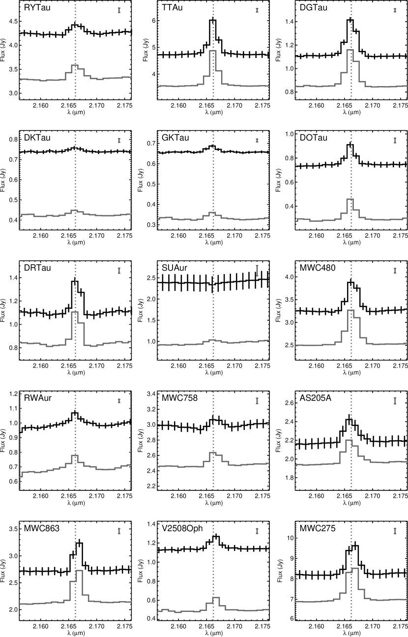
Figure 2: Flux versus wavelength for our sample objects measured with KI. This figure focuses on the spectral region around the Br$\gamma$ transition. The solid histogram shows the observed spectrum for the target, and the gray histogram shows the flux of the circumstellar component only. For clarity of presentation, we have not plotted the error bars associated with the circumstellar fluxes; the magnitudes of the uncertainties are indicated in the upper right corners. Dotted gray lines indicate the central (rest) wavelength of the Br$\gamma$ transition, 2.1662 $\mu$m.

Figure 2: continued.

Figure 10: $V^{2}$ observed with KI across the entire $K$-band for V1685 Cyg (solid curve) and AS 442 (dotted curve), illustrating the unusual spectral behavior of the V1685 Cyg visibilities. AS 442 is representative of other objects in our sample, and is chosen for this plot because it shared the same calibration as V1685 Cyg (Table Constraining the Sub-AU-Scale Distribution of Hydrogen and Carbon Monoxide Gas around Young Stars with the Keck Interferometer).

References

- Acke et al. (2005) Acke, B., van den Ancker, M. E., & Dullemond, C. P. 2005, A&A, 436, 209
- Bans & Königl (2012) Bans, A. & Königl, A. 2012, ApJ, 758, 100
- Beck et al. (2010) Beck, T. L., Bary, J. S., & McGregor, P. J. 2010, ApJ, 722, 1360
- Benisty et al. (2010) Benisty, M., Natta, A., Isella, A., Berger, J., Massi, F., Le Bouquin, J., Mérand, A., Duvert, G., Kraus, S., Malbet, F., Olofsson, J., Robbe-Dubois, S., Testi, L., Vannier, M., & Weigelt, G. 2010, A&A, 511, 74
- Berthoud (2008) Berthoud, M. G. 2008, PhD thesis, Cornell University
- Berthoud et al. (2007) Berthoud, M. G., Keller, L. D., Herter, T. L., Richter, M. J., & Whelan, D. G. 2007, ApJ, 660, 461
- Bertout et al. (2007) Bertout, C., Siess, L., & Cabrit, S. 2007, A&A, 473, L21
- Biscaya et al. (1997) Biscaya, A. M., Rieke, G. H., Narayanan, G., Luhman, K. L., & Young, E. T. 1997, ApJ, 491, 359
- Boden et al. (1998) Boden, A. F., Colavita, M. M., van Belle, G. T., & Shao, M. 1998, in Proc. SPIE Vol. 3350, p. 872-880, Astronomical Interferometry, Robert D. Reasenberg; Ed., 872–880
- Brittain et al. (2007) Brittain, S. D., Simon, T., Najita, J. R., & Rettig, T. W. 2007, ApJ, 659, 685
- Calvet et al. (2004) Calvet, N., Muzerolle, J., Briceño, C., Hernández, J., Hartmann, L., Saucedo, J. L., & Gordon, K. D. 2004, AJ, 128, 1294
- Carr (1989) Carr, J. S. 1989, ApJ, 345, 522
- Carr et al. (2004) Carr, J. S., Tokunaga, A. T., & Najita, J. 2004, ApJ, 603, 213
- Chini (1981) Chini, R. 1981, A&A, 99, 346
- Colavita et al. (2003) Colavita, M., Akeson, R., Wizinowich, P., Shao, M., Acton, S., Beletic, J., Bell, J., Berlin, J., Boden, A., Booth, A., Boutell, R., Chaffee, F., Chan, D., Chock, J., Cohen, R., Crawford, S., Creech-Eakman, M., Eychaner, G., Felizardo, C., Gathright, J., Hardy, G., Henderson, H., Herstein, J., Hess, M., Hovland, E., Hrynevych, M., Johnson, R., Kelley, J., Kendrick, R., Koresko, C., Kurpis, P., Le Mignant, D., Lewis, H., Ligon, E., Lupton, W., McBride, D., Mennesson, B., Millan-Gabet, R., Monnier, J., Moore, J., Nance, C., Neyman, C., Niessner, A., Palmer, D., Reder, L., Rudeen, A., Saloga, T., Sargent, A., Serabyn, E., Smythe, R., Stomski, P., Summers, K., Swain, M., Swanson, P., Thompson, R., Tsubota, K., Tumminello, A., van Belle, G., Vasisht, G., Vause, J., Walker, J., Wallace, K., & Wehmeier, U. 2003, ApJ, 592, L83
- Colavita (1999) Colavita, M. M. 1999, PASP, 111, 111
- Colavita & Wizinowich (2003) Colavita, M. M. & Wizinowich, P. L. 2003, in Interferometry for Optical Astronomy II. Edited by Wesley A. Traub. Proceedings of the SPIE, Volume 4838, pp. 79-88 (2003)., 79–88
- Colavita et al. (2013) Colavita, M. M., Wizinowich, P. L., Akeson, R. L., Ragland, S., Woillez, J. M., Millan-Gabet, R., Serabyn, E., Abajian, M., Acton, D. S., Appleby, E., Beletic, J. W., Beichman, C. A., Bell, J., Berkey, B. C., Berlin, J., Boden, A. F., Booth, A. J., Boutell, R., Chaffee, F. H., Chan, D., Chin, J., Chock, J., Cohen, R., Cooper, A., Crawford, S. L., Creech-Eakman, M. J., Dahl, W., Eychaner, G., Fanson, J. L., Felizardo, C., Garcia-Gathright, J. I., Gathright, J. T., Hardy, G., Henderson, H., Herstein, J. S., Hess, M., Hovland, E. E., Hrynevych, M. A., Johansson, E., Johnson, R. L., Kelley, J., Kendrick, R., Koresko, C. D., Kurpis, P., Le Mignant, D., Lewis, H. A., Ligon, E. R., Lupton, W., McBride, D., Medeiros, D. W., Mennesson, B. P., Moore, J. D., Morrison, D., Nance, C., Neyman, C., Niessner, A., Paine, C. G., Palmer, D. L., Panteleeva, T., Papin, M., Parvin, B., Reder, L., Rudeen, A., Saloga, T., Sargent, A., Shao, M., Smith, B., Smythe, R. F., Stomski, P., Summers, K. R., Swain, M. R., Swanson, P., Thompson, R., Tsubota, K., Tumminello, A., Tyau, C., van Belle, G. T., Vasisht, G., Vause, J., Vescelus, F., Walker, J., Wallace, J. K., Wehmeier, U., & Wetherell, E. 2013, PASP, 125, 1226
- Corcoran & Ray (1997) Corcoran, M. & Ray, T. P. 1997, A&A, 321, 189
- Dullemond et al. (2001) Dullemond, C. P., Dominik, C., & Natta, A. 2001, ApJ, 560, 957
- Dullemond & Monnier (2010) Dullemond, C. P. & Monnier, J. D. 2010, ARA&A, 48, 205
- Eisner (2007) Eisner, J. A. 2007, Nature, 447, 562
- Eisner et al. (2007a) Eisner, J. A., Chiang, E. I., Lane, B. F., & Akeson, R. L. 2007a, ApJ, 657, 347
- Eisner et al. (2007b) Eisner, J. A., Graham, J. R., Akeson, R. L., Ligon, E. R., Colavita, M. M., Basri, G., Summers, K., Ragland, S., & Booth, A. 2007b, ApJ, 654, L77
- Eisner et al. (2009) Eisner, J. A., Graham, J. R., Akeson, R. L., & Najita, J. 2009, ApJ, 692, 309
- Eisner & Hillenbrand (2011) Eisner, J. A. & Hillenbrand, L. A. 2011, ApJ, 738, 9
- Eisner et al. (2005) Eisner, J. A., Hillenbrand, L. A., White, R. J., Akeson, R. L., & Sargent, A. I. 2005, ApJ, 623, 952
- Eisner et al. (2007c) Eisner, J. A., Hillenbrand, L. A., White, R. J., Bloom, J. S., Akeson, R. L., & Blake, C. H. 2007c, ApJ, 669, 1072
- Eisner et al. (2004) Eisner, J. A., Lane, B. F., Hillenbrand, L., Akeson, R., & Sargent, A. 2004, ApJ, 613, 1049
- Eisner et al. (2010) Eisner, J. A., Monnier, J. D., Woillez, J., Akeson, R. L., Millan-Gabet, R., Graham, J. R., Hillenbrand, L. A., Pott, J., Ragland, S., & Wizinowich, P. 2010, ApJ, 718, 774
- Eisner et al. (2013) Eisner, J. A., Rieke, G. H., Rieke, M. J., Flaherty, K. M., Arnold, T. J., Stone, J. M., Cortes, S. R., Cox, E., Hawkins, C., Cole, A., Zajac, S., & Rudolph, A. L. 2013, MNRAS, 434, 407
- Folha & Emerson (2001) Folha, D. F. M. & Emerson, J. P. 2001, A&A, 365, 90
- Glassgold et al. (2004) Glassgold, A. E., Najita, J., & Igea, J. 2004, ApJ, 615, 972
- Gorti & Hollenbach (2008) Gorti, U. & Hollenbach, D. 2008, ApJ, 683, 287
- Hamann (1994) Hamann, F. 1994, ApJS, 93, 485
- Hartigan et al. (1995) Hartigan, P., Edwards, S., & Ghandour, L. 1995, ApJ, 452, 736
- Hartigan et al. (1986) Hartigan, P., Mundt, R., & Stocke, J. 1986, AJ, 91, 1357
- Hauschildt et al. (1999) Hauschildt, P. H., Allard, F., & Baron, E. 1999, ApJ, 512, 377
- Herbig & Jones (1983) Herbig, G. H. & Jones, B. F. 1983, AJ, 88, 1040
- Herbig et al. (2003) Herbig, G. H., Petrov, P. P., & Duemmler, R. 2003, ApJ, 595, 384
- Herczeg & Hillenbrand (2014) Herczeg, G. J. & Hillenbrand, L. A. 2014, ArXiv e-prints
- Isella & Natta (2005) Isella, A. & Natta, A. 2005, A&A, 438, 899
- Isella et al. (2008) Isella, A., Tatulli, E., Natta, A., & Testi, L. 2008, A&A, 483, L13
- Kenyon et al. (1994) Kenyon, S. J., Dobrzycka, D., & Hartmann, L. 1994, AJ, 108, 1872
- Königl (1991) Königl, A. 1991, ApJ, 370, L39
- Konigl & Pudritz (2000) Konigl, A. & Pudritz, R. E. 2000, Protostars and Planets IV, 759
- Kraus et al. (2008a) Kraus, S., Hofmann, K.-H., Benisty, M., Berger, J.-P., Chesneau, O., Isella, A., Malbet, F., Meilland, A., Nardetto, N., Natta, A., Preibisch, T., Schertl, D., Smith, M., Stee, P., Tatulli, E., Testi, L., & Weigelt, G. 2008a, A&A, 489, 1157
- Kraus et al. (2008b) Kraus, S., Preibisch, T., & Ohnaka, K. 2008b, ApJ, 676, 490
- Kuhi (1964) Kuhi, L. V. 1964, ApJ, 140, 1409
- Kurosawa et al. (2006) Kurosawa, R., Harries, T. J., & Symington, N. H. 2006, MNRAS, 370, 580
- Lynden-Bell & Pringle (1974) Lynden-Bell, D. & Pringle, J. E. 1974, MNRAS, 168, 603
- Malbet et al. (2007) Malbet, F., Benisty, M., de Wit, W.-J., Kraus, S., Meilland, A., Millour, F., Tatulli, E., Berger, J.-P., Chesneau, O., Hofmann, K.-H., Isella, A., Natta, A., Petrov, R. G., Preibisch, T., Stee, P., Testi, L., Weigelt, G., Antonelli, P., Beckmann, U., Bresson, Y., Chelli, A., Dugué, M., Duvert, G., Gennari, S., Glück, L., Kern, P., Lagarde, S., Le Coarer, E., Lisi, F., Perraut, K., Puget, P., Rantakyrö, F., Robbe-Dubois, S., Roussel, A., Zins, G., Accardo, M., Acke, B., Agabi, K., Altariba, E., Arezki, B., Aristidi, E., Baffa, C., Behrend, J., Blöcker, T., Bonhomme, S., Busoni, S., Cassaing, F., Clausse, J.-M., Colin, J., Connot, C., Delboulbé, A., Domiciano de Souza, A., Driebe, T., Feautrier, P., Ferruzzi, D., Forveille, T., Fossat, E., Foy, R., Fraix-Burnet, D., Gallardo, A., Giani, E., Gil, C., Glentzlin, A., Heiden, M., Heininger, M., Hernandez Utrera, O., Kamm, D., Kiekebusch, M., Le Contel, D., Le Contel, J.-M., Lesourd, T., Lopez, B., Lopez, M., Magnard, Y., Marconi, A., Mars, G., Martinot-Lagarde, G., Mathias, P., Mège, P., Monin, J.-L., Mouillet, D., Mourard, D., Nussbaum, E., Ohnaka, K., Pacheco, J., Perrier, C., Rabbia, Y., Rebattu, S., Reynaud, F., Richichi, A., Robini, A., Sacchettini, M., Schertl, D., Schöller, M., Solscheid, W., Spang, A., Stefanini, P., Tallon, M., Tallon-Bosc, I., Tasso, D., Vakili, F., von der Lühe, O., Valtier, J.-C., Vannier, M., & Ventura, N. 2007, A&A, 464, 43
- McLean et al. (2003) McLean, I. S., McGovern, M. R., Burgasser, A. J., Kirkpatrick, J. D., Prato, L., & Kim, S. S. 2003, ApJ, 596, 561
- Mendigutía et al. (2011) Mendigutía, I., Calvet, N., Montesinos, B., Mora, A., Muzerolle, J., Eiroa, C., Oudmaijer, R. D., & Merín, B. 2011, A&A, 535, A99
- Monin et al. (1998) Monin, J.-L., Menard, F., & Duchene, G. 1998, A&A, 339, 113
- Monnier et al. (2006) Monnier, J. D., Berger, J.-P., Millan-Gabet, R., Traub, W. A., Schloerb, F. P., Pedretti, E., Benisty, M., Carleton, N. P., Haguenauer, P., Kern, P., Labeye, P., Lacasse, M. G., Malbet, F., Perraut, K., Pearlman, M., & Zhao, M. 2006, ApJ, 647, 444
- Monnier & Millan-Gabet (2002) Monnier, J. D. & Millan-Gabet, R. 2002, ApJ, 579, 694
- Monnier et al. (2005) Monnier, J. D., Millan-Gabet, R., Billmeier, R., Akeson, R. L., Wallace, D., Berger, J.-P., Calvet, N., D’Alessio, P., Danchi, W. C., Hartmann, L., Hillenbrand, L. A., Kuchner, M., Rajagopal, J., Traub, W. A., Tuthill, P. G., Boden, A., Booth, A., Colavita, M., Gathright, J., Hrynevych, M., Le Mignant, D., Ligon, R., Neyman, C., Swain, M., Thompson, R., Vasisht, G., Wizinowich, P., Beichman, C., Beletic, J., Creech-Eakman, M., Koresko, C., Sargent, A., Shao, M., & van Belle, G. 2005, ApJ, 624, 832
- Mundt & Eislöffel (1998) Mundt, R. & Eislöffel, J. 1998, AJ, 116, 860
- Muzerolle et al. (2003) Muzerolle, J., Calvet, N., Hartmann, L., & D’Alessio , P. 2003, ApJ, 597, L865
- Muzerolle et al. (1998) Muzerolle, J., Hartmann, L., & Calvet, N. 1998, AJ, 116, 2965
- Najita et al. (1996a) Najita, J., Carr, J. S., Glassgold, A. E., Shu, F. H., & Tokunaga, A. T. 1996a, ApJ, 462, 919
- Najita et al. (1996b) Najita, J., Carr, J. S., & Tokunaga, A. T. 1996b, ApJ, 456, 292
- Najita et al. (2007) Najita, J. R., Carr, J. S., Glassgold, A. E., & Valenti, J. A. 2007, in Protostars and Planets V, B. Reipurth, D. Jewitt, and K. Keil (eds.), University of Arizona Press, Tucson, 951 pp., 2007., p.507-522, ed. B. Reipurth, D. Jewitt, & K. Keil, 507–522
- Najita et al. (2009) Najita, J. R., Doppmann, G. W., Carr, J. S., Graham, J. R., & Eisner, J. A. 2009, ApJ, 691, 738
- Najita et al. (2000) Najita, J. R., Edwards, S., Basri, G., & Carr, J. 2000, Protostars and Planets IV, 457
- Palla & Stahler (1993) Palla, F. & Stahler, S. W. 1993, ApJ, 418, 414
- Perryman et al. (1997) Perryman, M. A. C., Lindegren, L., Kovalevsky, J., Hoeg, E., Bastian, U., Bernacca, P. L., Crézé, M., Donati, F., Grenon, M., van Leeuwen, F., van der Marel, H., Mignard, F., Murray, C. A., Le Poole, R. S., Schrijver, H., Turon, C., Arenou, F., Froeschlé, M., & Petersen, C. S. 1997, A&A, 323, L49
- Prato et al. (2003) Prato, L., Greene, T. P., & Simon, M. 2003, ApJ, 584, 853
- Pyo et al. (2003) Pyo, T.-S., Kobayashi, N., Hayashi, M., Terada, H., Goto, M., Takami, H., Takato, N., Gaessler, W., Usuda, T., Yamashita, T., Tokunaga, A. T., Hayano, Y., Kamata, Y., Iye, M., & Minowa, Y. 2003, ApJ, 590, 340
- Rothman et al. (2005) Rothman, L. S., Jacquemart, D., Barbe, A., Benner, D. C., Birk, M., Brown, L. R., Carleer, M. R., Chackerian, C., Chance, K., Coudert, L. H., Dana, V., Devi, V. M., Flaud, J. M., Gamache, R. R., Goldman, A., Hartmann, J. M., Jucks, K. W., Maki, A. G., Mandin, J. Y., Massie, S. T., Orphal, J., Perrin, A., Rinsland, C. P., Smith, M. A. H., Tennyson, J., Tolchenov, R. N., Toth, R. A., Vander Auwera, J., Varanasi, P., & Wagner, G. 2005, Journal of Quantitative Spectroscopy and Radiative Transfer, 96, 139
- Shu et al. (1994) Shu, F., Najita, J., Ostriker, E., Wilkin, F., Ruden, S., & Lizano, S. 1994, ApJ, 429, 781
- Tannirkulam et al. (2008) Tannirkulam, A., Monnier, J. D., Millan-Gabet, R., Harries, T. J., Pedretti, E., ten Brummelaar, T. A., McAlister, H., Turner, N., Sturmann, J., & Sturmann, L. 2008, ApJ, 677, L51
- Tatulli et al. (2007) Tatulli, E., Isella, A., Natta, A., Testi, L., Marconi, A., Malbet, F., Stee, P., Petrov, R. G., Millour, F., Chelli, A., Duvert, G., Antonelli, P., Beckmann, U., Bresson, Y., Dugué, M., Gennari, S., Glück, L., Kern, P., Lagarde, S., Le Coarer, E., Lisi, F., Perraut, K., Puget, P., Rantakyrö, F., Robbe-Dubois, S., Roussel, A., Weigelt, G., Zins, G., Accardo, M., Acke, B., Agabi, K., Altariba, E., Arezki, B., Aristidi, E., Baffa, C., Behrend, J., Blöcker, T., Bonhomme, S., Busoni, S., Cassaing, F., Clausse, J.-M., Colin, J., Connot, C., Delboulbé, A., Domiciano de Souza, A., Driebe, T., Feautrier, P., Ferruzzi, D., Forveille, T., Fossat, E., Foy, R., Fraix-Burnet, D., Gallardo, A., Giani, E., Gil, C., Glentzlin, A., Heiden, M., Heininger, M., Hernandez Utrera, O., Hofmann, K.-H., Kamm, D., Kiekebusch, M., Kraus, S., Le Contel, D., Le Contel, J.-M., Lesourd, T., Lopez, B., Lopez, M., Magnard, Y., Mars, G., Martinot-Lagarde, G., Mathias, P., Mège, P., Monin, J.-L., Mouillet, D., Mourard, D., Nussbaum, E., Ohnaka, K., Pacheco, J., Perrier, C., Rabbia, Y., Rebattu, S., Reynaud, F., Richichi, A., Robini, A., Sacchettini, M., Schertl, D., Schöller, M., Solscheid, W., Spang, A., Stefanini, P., Tallon, M., Tallon-Bosc, I., Tasso, D., Vakili, F., von der Lühe, O., Valtier, J.-C., Vannier, M., & Ventura, N. 2007, A&A, 464, 55
- Tatulli et al. (2008) Tatulli, E., Malbet, F., Ménard, F., Gil, C., Testi, L., Natta, A., Kraus, S., Stee, P., & Robbe-Dubois, S. 2008, A&A, 489, 1151
- Thi et al. (2005) Thi, W.-F., van Dalen, B., Bik, A., & Waters, L. B. F. M. 2005, A&A, 430, L61
- Weidenschilling (1977) Weidenschilling, S. J. 1977, Ap&SS, 51, 153
- Weigelt et al. (2011) Weigelt, G., Grinin, V. P., Groh, J. H., Hofmann, K.-H., Kraus, S., Miroshnichenko, A. S., Schertl, D., Tambovtseva, L. V., Benisty, M., Driebe, T., Lagarde, S., Malbet, F., Meilland, A., Petrov, R., & Tatulli, E. 2011, A&A, 527, A103
- White & Ghez (2001) White, R. J. & Ghez, A. M. 2001, ApJ, 556, 265
- Woillez et al. (2012) Woillez, J., Akeson, R., Colavita, M., Eisner, J., Millan-Gabet, R., Monnier, J., Pott, J.-U., Ragland, S., Wizinowich, P., Abajian, M., Appleby, E., Berkey, B., Cooper, A., Felizardo, C., Herstein, J., Hrynevych, M., Medeiros, D., Morrison, D., Panteleeva, T., Smith, B., Summers, K., Tsubota, K., Tyau, C., & Wetherell, E. 2012, PASP, 124, 51
- Woillez et al. (2014) Woillez, J., Wizinowich, P., Akeson, R., Colavita, M., Eisner, J., Millan-Gabet, R., Monnier, J. D., Pott, J.-U., & Ragland, S. 2014, ApJ, 783, 104