Image patch analysis and clustering of sunspots: a dimensionality reduction approach

Abstract

Sunspots, as seen in white light or continuum images, are associated with regions of high magnetic activity on the Sun, visible on magnetogram images. Their complexity is correlated with explosive solar activity and so classifying these active regions is useful for predicting future solar activity. Current classification of sunspot groups is visually based and suffers from bias. Supervised learning methods can reduce human bias but fail to optimally capitalize on the information present in sunspot images. This paper uses two image modalities (continuum and magnetogram) to characterize the spatial and modal interactions of sunspot and magnetic active region images and presents a new approach to cluster the images. Specifically, in the framework of image patch analysis, we estimate the number of intrinsic parameters required to describe the spatial and modal dependencies, the correlation between the two modalities and the corresponding spatial patterns, and examine the phenomena at different scales within the images. To do this, we use linear and nonlinear intrinsic dimension estimators, canonical correlation analysis, and multiresolution analysis of intrinsic dimension.

Index Terms—  sunspot, active region, intrinsic dimension, CCA, clustering

1 Introduction

Sunspots are associated with active regions, which are areas of locally increased magnetic flux on the Sun. The morphology of sunspot groups and associated active regions is correlated with the incidence of solar flares [1]. The current practice for identifying and classifying sunspot groups is based on the Mount Wilson classification scheme, which categorizes them by eye based on morphological criteria present in continuum and magnetogram images. Such visual classification introduces bias stemming from the artificial and subjective nature of the discrete categorization. It also makes the study of the sunspot group’s dynamic behaviour impractical.

Recent works [2, 3] have attempted to reproduce the Mount Wilson classification through automated procedures while [4] has employed multiresolution analysis to differentiate the various types of active regions. While these approaches reduce the human bias, they do not use the information present in sunspot images in an optimal way. This paper presents for the first time a spatial correlation and intrinsic dimension analysis of sunspot images and a new approach to cluster the images. We use two image modalities (continuum and magnetogram) to characterize their spatial and modal interactions for improved sunspot classification. To do this, we first address three questions for umbral and penumbral regions of the sunspot. 1) How many intrinsic parameters or degrees of freedom are required to describe the spatial and modal dependencies? 2) What correlation exists between the two modalities and what spatial patterns produce that correlation? 3) What phenomena exist at different scales within the images? We use this information to cluster the images by clustering dictionaries learned from each image.

The paper is organized as follows. In Sec. 2, a description of the dataset is provided. In Sec. 3, the intrinsic dimension of the joint image is estimated using both nonlinear and linear methods. We also perform a multiresolution analysis (MRA) of intrinsic dimension. We then identify complex spatial and modal interactions at different scales that are not visible to the naked eye by using canonical correlation analysis (CCA) in Sec. 4. Section 5 then presents our clustering approaches and results.

MRA has been used for many image applications including denoising and reconstruction [5], segmentation [6], and representation [7]. Many of these methods use a basis transformation and then a linear decomposition of the transformed data. Our case differs in that the sunspot images are vector valued (two modalities), possibly non-linear, and nonstationary so standard linear MRA may not be sufficient to capture the interactions between the two modalities.

2 Data

The data used in this study are taken from the MDI instrument [8] on board the SOHO Spacecraft. The active regions of the Sun are observed using level 1.8 continuum (cont) and level 1.8 magnetogram (mag) images. Active regions are selected within $30$ degrees of the solar meridian to avoid strong projection effects. Expertly generated masks marking the location of the umbra and penumbra of the sunspots are available for each set of images [9]. Information about the sunspot groups such as Mount Wilson class labels, Zurich class labels, and sunspot group longitudinal extent comes from the Solar Region Summary reports compiled by the Space Weather Prediction Center of NOAA http://www.swpc.noaa.gov/ftpdir/forecasts/SRS/.

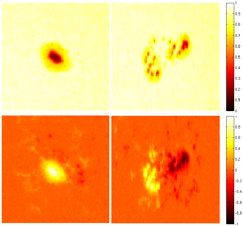
Fig. 1: Cont (top) and mag (bottom) images. Left to right: single spot, multiple spots.

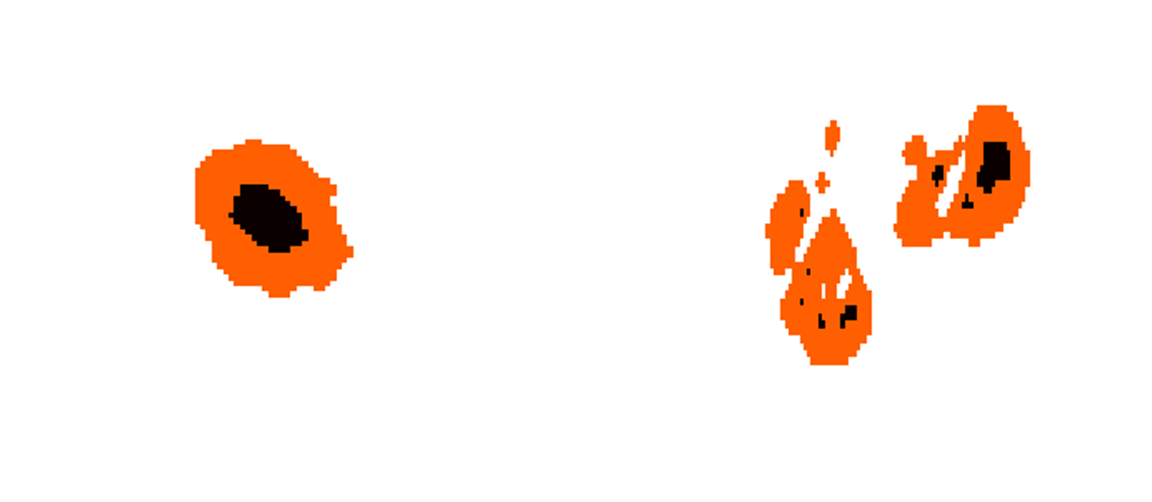
Fig. 2: Masks for the single spot and multiple spot images extracted by solar sunspot experts. Interior = umbra, exterior = penumbra.

Similarly to [10, 11, 12], we use image patch features to account for spatial dependencies using square patches of pixels. Thus if an image has $n$ pixels and we use a $3\times 3$ patch, the corresponding cont data matrix $X$ is $9\times n$ where the $i$th column contains the pixels in the patch centered at the $i$th pixel. The mag data matrix $Y$ is formed in the same way and the full data matrix is $Z=\left(\begin{array}[]{cc}X^{T}&Y^{T}\end{array}\right)^{T}$.

While we have applied our analysis to a large corpus of sunspot images, two specific images are used to illustrate our results: a region with a single sunspot and a region with intense magnetic activity and multiple sunspots. The images and masks are given in Figs. 1 and 2, respectively.

3 Intrinsic Dimension Estimation

To determine the number of intrinsic parameters or degrees of freedom required to describe the spatial and modal dependencies, we estimate the local intrinsic dimension of the joint $3\times 3$ patches, which lie in an extrinsic Euclidean space of 18 dimensions. We investigate two different methods for estimation of intrinsic dimension: the first is appropriate to linear subspaces while the second is appropriate to any (linear or non-linear) smooth subspace. The linear method we use is principal component analysis (PCA). PCA finds a set of linearly uncorrelated vectors (principal components) that can be used to represent the data. The principal components are the eigenvectors of the covariance matrix $\Sigma=\left(\begin{array}[]{cc}\Sigma_{\mathbf{xx}}&\Sigma_{\mathbf{xy}}\\ \Sigma_{\mathbf{yx}}&\Sigma_{\mathbf{yy}}\end{array}\right),$ where $\mathbf{x}$ and $\mathbf{y}$ are random vectors, $\mathbf{x}$ is a patch from the cont image, and $\mathbf{y}$ is the corresponding patch from the mag image. The eigenvalues indicate the amount of variance accounted for by the corresponding principal component. A linear estimate of intrinsic dimension is the number of principal components that are required to explain a certain percentage of the variance. To account for differences between the umbra, penumbra, and background, PCA is performed separately on those areas using the masks provided in Fig. 2.

The nonlinear method we use is a $k$-NN graph approach with neighborhood smoothing [13] which is as follows. For a set of independently identically distributed random vectors $\mathbf{Z}_{n}=\{z_{1},\dots,z_{n}\}$ with values in a compact subset of $\mathbb{R}^{d}$, the $k$-nearest neighbors of $z_{i}$ in $\mathbf{Z}_{n}$ are the $k$ points in $\mathbf{Z}_{n}\backslash\{z_{i}\}$ closest to $z_{i}$ as measured by the Euclidean distance $||\cdot||$. The $k$-NN graph is then formed by assigning edges between a point in $\mathbf{Z}_{n}$ and its $k$-nearest neighbors and has total edge length defined as

$$L_{\gamma,k}(\mathbf{Z}_{n})=\sum_{i=1}^{n}\sum_{z\in\mathcal{N}_{k,i}}||z-z_{i}||^{\gamma},$$

where $\gamma>0$ is a power weighting constant and $\mathcal{N}_{k,i}$ is the set of $k$ nearest neighbors of $z_{i}.$ The asymptotics of $L_{\gamma,k}(\mathbf{Z}_{n})$ are given in the following theorem [14]:

Theorem 1

Let $(\mathcal{M},g)$ be a compact smooth Riemann $m$-dimensional manifold. Suppose $z_{1},\dots,z_{n}$ are i.i.d. random elements of $\mathcal{M}$ with bounded density $f$ relative to $\mu_{g}$. Assume that $m\geq 2$, $1\leq\gamma<m$ and define $\alpha=(m-\gamma)/m$. Then

$$\lim_{n\rightarrow\infty}\frac{L_{\gamma,k}(\mathbf{Z}_{n})}{n^{\alpha}}=\beta_{m,L_{\gamma}}\int_{\mathcal{M}}f^{\alpha}(z)\mu_{g}(dz)\text{ }a.s.,$$

where $\beta_{m,L_{\gamma}}$ is a constant independent of $f$ and $\mathcal{M}$.

Theorem 1 says that the total edge length of the $k$-NN graph increases in $n$ at a sublinear rate $n^{\alpha}$ with $\alpha<1$, where $\alpha$ is related to the intrinsic dimension $m$ of the manifold $\mathcal{M}.$ The sublinear slope is closely related to the Rényi entropy $H_{\alpha}(f)=(1-\alpha)\ln\int_{\mathcal{M}}f^{\alpha}(z)\mu_{g}(dz)$ of the density $f$ on the manifold. Then for large $n$:

$$L_{\gamma,k}(\mathbf{Z}_{n})=n^{\alpha(m)}c+\epsilon_{n},$$

where $c$ is a constant with respect to $\alpha(m)$ that depends on the Renyi entropy of the distribution of the manifold and $\epsilon_{n}$ is an error term that decreases to zero a.s. as $n\rightarrow\infty$ [14]. Using this expression, a global intrinsic dimension estimate $\hat{m}$ is found using non-linear least squares over different values of $n$ [13].

To find a local estimate of dimension at a point $z_{i}$, the algorithm is run over a smaller neighborhood about $z_{i}.$ However, this can result in highly variable estimates of dimension for nearby points. This variance can be reduced by smoothing the intrinsic dimension estimate by majority voting in a neighborhood of $z_{i}.$ Specifically,

$$\hat{m}(z_{i})=\hat{m}(i)=\arg\max_{l}\sum_{z_{j}\in\mathcal{N}_{i}}1(\hat{m}(z_{j})=l),$$

where $1(\cdot)$ is the indicator function and $\mathcal{N}_{i}$ is the neighborhood of $z_{i}$ [13]. We use $|\mathcal{N}_{i}|=6$.

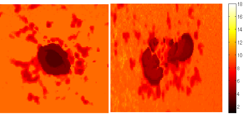
Fig. 3: $k$-NN estimate of local intrinsic dimension ($\hat{m}(i)$, where $i$ indexes over image pixels) of the single sunspot (left), and multiple sunspot (right) images. The standard deviation across iterations for each pixel is generally less than 1.

To account for variance due to random paths, we run the algorithm 20 times per image. Figure 3 gives the mean of the estimated local dimension for each image using a $3\times 3$ patch. Most of the background of the single sunspot image has estimated dimension varying between $\hat{m}=9$ or 10, which is consistent with estimates obtained throughout pure background images (not shown). However, there are regions with magnetic activity outside of the main sunspot (magnetic fragments) that have lower estimated dimension $\hat{m}\approx 5,$ or $6$. The sunspot also has lower dimension ($\hat{m}\approx 3-5$) than the background. This is expected since the background has less structure compared to the sunspots and magnetic fragments. Similar results are obtained for the multi-spot image.

Table 1 gives the estimated intrinsic dimension for 20 images (10 with a single spot, 10 with multiple spots) extracted from the corpus using both PCA and the $k$-NN method. For the $k$-NN method, the algorithm is run 20 times per image and the mean is reported for each region. For PCA, the intrinsic dimension based on a 97% threshold averaged across images is reported. With the exception of the umbra for single sunspots, the 97% PCA result is within one standard deviation of the $k$-NN mean. Thus depending on the precision required, linear methods may be sufficient to represent the spatial and modal dependencies within most of the images. PCA and $k$-NN estimates are in closer agreement for multiple sunspot images than for single sunspots. Since the multiple sunspot images often have more magnetic fragments in the background than single sunspots, this suggests that linear methods may perform better at representing these regions compared to pure background.

	Background	Penumbra	Umbra
Single Spot $k$-NN	8.9	4.5	3.4
Single Spot PCA	10.1	4.3	6.3
Multiple Spots $k$-NN	8.6	4.8	4.0
Multiple Spots PCA	8.9	4.8	3.4

Table 1: Estimated intrinsic dimension for multiple images with single sunspots and multiple sunspots using $k$-NN or PCA. PCA values correspond to a 97% threshold.

To explore the existence of different phenomena at different scales, we perform MRA on intrinsic dimension since the intrinsic dimension estimates indicate the areas where the two modalities are most correlated. Each scale (layer) is produced using a Haar wavelet decomposition and reconstruction. We estimate the intrinsic dimension at each layer for single sunspots using the two methods discussed in Sec. 3. Both methods are used with $3\times 3$ patches. At the 0th and 1st layers, we average the results from three similar images. At the 2nd layer, we analyze the combined data to ensure enough samples within each region. The results using both PCA and the $k$-NN method are given in Fig. 4.

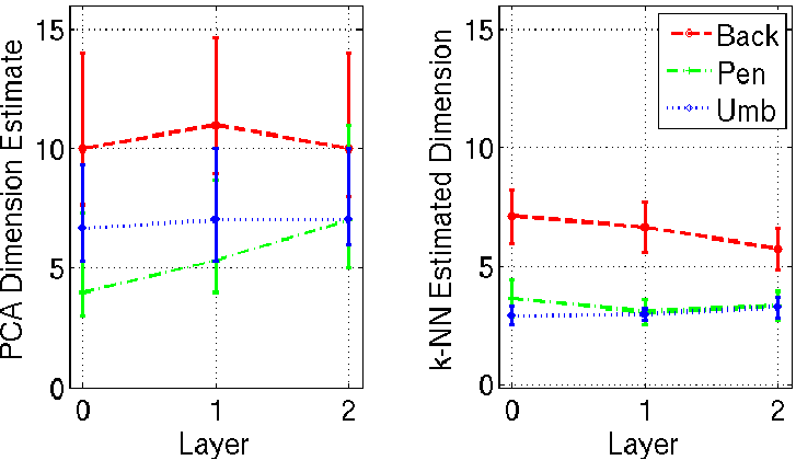
Fig. 4: Estimated intrinsic dimension using PCA (left) and the average $\hat{m}$ using the $k$-NN method (right) within each region as a function of scale for three single sunspot images. The error bars correspond to a single standard deviation for the $k$-NN method and to the 95% and 99% thresholds for PCA (plot corresponds to 97%).

The results for the initial resolution are consistent with Table 1. As scale increases, $\hat{m}$ decreases within the background while the PCA estimate increases initially. Using the Jonckheere-Terpstra trend (Jtrend) test [15] shows that both relationships are significant. Since noise generally has a higher dimension, this suggests that increasing the scale in the background effectively denoises the data for the $k$-NN estimate. Within the penumbra, $\hat{m}$ decreases initially and then increases while the PCA estimate increases consistently. Within the umbra, both $\hat{m}$ and the PCA estimate increase gradually. The Jtrend test shows that all of these relationships are significant except for the umbra PCA estimate. This is similar to [16] where the entropy of certain image textures is found to be generally increasing but nonmonotonically with scale.

Figure 5 shows $\hat{m}$ of the single sunspot image at the different scales. The background in the 1st layer appears to be a denoised version of the estimate at the original resolution. Some of the magnetic fragments are preserved and the remaining background is more uniform. Other trends in the images are consistent with Fig. 4. Similar results are obtained for images with multiple sunspots.

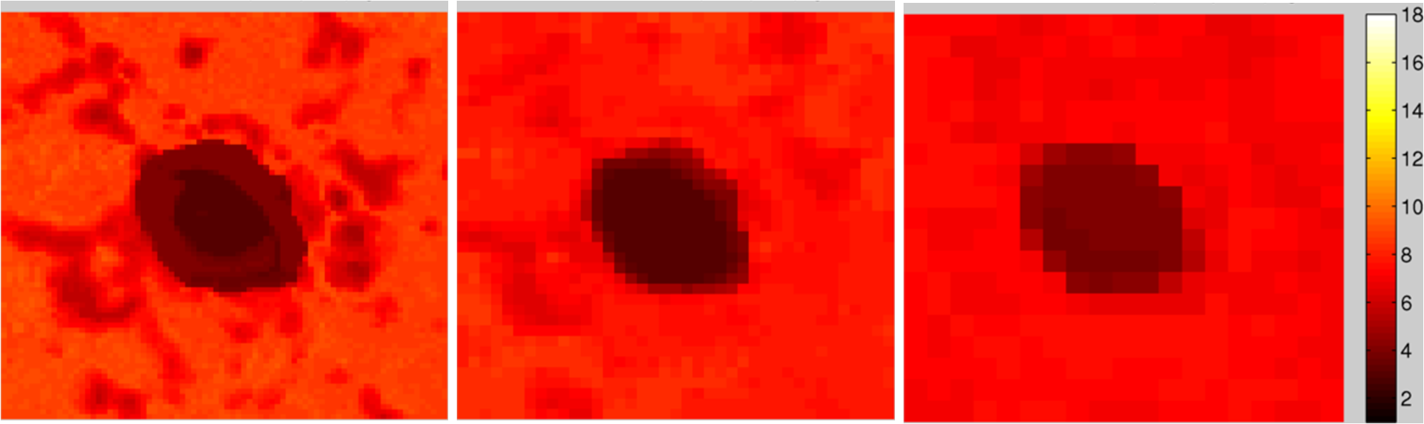
Fig. 5: Local estimated intrinsic dimension ($\hat{m}(i)$) of the single sunspot image at different scales. L to R: 0th, 1st, and 2nd layers.

4 Correlation of Cont and Mag Images

As the results in the previous section indicate that linear methods may be sufficient to represent the spatial and modal dependencies within a sunspot, we analyze the linear correlation over patches. We do this by using canonical correlation analysis (CCA). We perform this analysis within the background, the umbra, and the penumbra of each image while using different patch sizes.

CCA finds vectors $a_{i}$ and $b_{i}$ such that the correlation $\rho_{i}=\text{corr}(a_{i}^{T}\mathbf{x},b_{i}^{T}\mathbf{y})$ is maximized and the pair of random variables $u_{i}=a_{i}^{T}\mathbf{x}$ and $v_{i}=b_{i}^{T}\mathbf{y}$ are uncorrelated with all other pairs $u_{j}$ and $v_{j}$, $j\neq i$. The variables $u_{i}$ and $v_{i}$ are called the $i$th pair of canonical variables. The solution $a_{i}$ is the $i$th eigenvector of the matrix $\Sigma_{\mathbf{xx}}^{-1}\Sigma_{\mathbf{xy}}\Sigma_{\mathbf{yy}}^{-1}\Sigma_{\mathbf{yx}}$. The vector $b_{i}$ is found similarly [17].

The variables $u_{1}$ and $v_{1}$ for the single sunspot image using different patch sizes are given in Fig. 6. $u_{1}$ and $v_{1}$ are calculated separately for the background, umbra, and penumbra and the first canonical correlation is approximately $0.25$, $0.95$, and $0.9$ respectively using a $3\times 3$ patch. The areas with highest correlation (in magnitude) are primarily around the edges of the penumbra and umbra as well as the magnetic fragments. Some of the magnetic fragments are highly positively correlated while others are highly negatively correlated. This correlation suggests that classification algorithms should process both modalities together for optimal performance.

As patch size is increased, the contrast in the images generally increases at the expense of blurred edges. Thus multiple patch sizes may be used to identify the regions with greatest correlation.

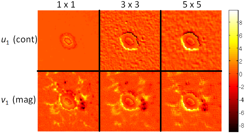
Fig. 6: Canonical variable images using different patch sizes of the single sunspot image. Left to right: $1\times 1$, $3\times 3$, and $5\times 5$ patch. $u_{1}$ (top) and $v_{1}$ (bottom).

5 Clustering of sunspot images

We applied the image patch analysis discussed in Secs. 2-4 to unsupervised classification of sunspot images over the corpus of sunspot images. First, we extract a 320 square pixel region centered on each sunspot group. This results in 509 sunspot group images taken from about 400 pairs of images. We then form a data matrix for each sunspot group image using either pixel patches as described previously or the canonical variables $u_{i}$ and $v_{i}.$ Next we use dictionary learning on each individual data matrix. Our intrinsic dimension analysis of the corpus in Sec. 3 implies that the umbra, penumbra and magnetic fragments of the images can be well approximated linearly (via PCA) by 7 dimensions or less. Hence we use linear dictionary learning models and restrict the size of the dictionaries to be less than or equal to 7. We then treat each learned dictionary as a single vector and use spectral clustering methods on these vectors to classify the images into distinct groups.

The clustering algorithm we use is the EAC-DC method in [18] which scales well for clustering in high dimensions. EAC-DC clusters the data by using a metric based on the hitting time of two Minimal Spanning Trees (MST) grown sequentially from a pair of points. Consensus spectral clustering is then applied to an ensemble of the resulting dual rooted MSTs. This method was found to be robust and competitive with other clustering algorithms [18].

To aid in interpreting our clustering results, we compare them to the Mount Wilson labels with five classes: beta (1), alpha (2), beta-gamma (3), beta-gamma-delta (4), and beta-delta (5). The normalized mutual information (NMI) and adjusted Rand index (ARI) of the Mount Wilson labels and our results using PCA to learn the dictionary from image patches are $0.11$ and $0.03$, respectively. This low correspondence is expected since our clustering approach is based on local image patch features while the Mount Wilson labeling scheme focuses on global features e.g. the polarities present in the group and whether they can be separated spatially with a line.

To visualize the images in low dimension, we projected the similarity matrix created by the dual rooted MSTs onto the eigenvectors of the normalized Laplacian of the similarity matrix, i.e. multidimensional scaling [19]. Figure 7 gives a scatter plot of $c_{1}$ vs. $c_{2}$ (top) and $c_{3}$ vs. $c_{2}$ (bottom) where $c_{i}$ is the projection onto the $i$th eigenvector. The points are labeled according to the clusters (left) and the Mount Wilson labels (right). The plots show that three clear groups of points are clearly visible and linearly separable. The plots on the left show that clusters 1, 4, and 5 are connected tightly while clusters 2 and 3 appear to be disconnected. In contrast, the Mount Wilson labels are mixed throughout the three point clouds. However, there are still some patterns present. For example, there are small groups of alpha images (labeled 2) located on the left and right ends of the top and bottom point clouds in the top right plot suggesting that our clustering method finds distinct features of the images.

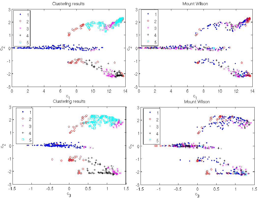
Fig. 7: Plots of $c_{1}$ vs. $c_{2}$ (top) and $c_{3}$ vs. $c_{2}$ (bottom) where $c_{i}$ is the projection of the similarity matrix onto the $i$th eigenvector of the normalized Laplacian. Points are labeled according to our clusters using the EAC-DC algorithm (left) and the Mount Wilson labels (right). This shows that the intrinsic spatial features are quite different from those used in the Mount Wilson classifications.

There is also some correlation with our results and the longitudinal extent of the sunspot group: cluster 2 includes only smaller groups with longitudinal extent less than 5 degrees while cluster 3 includes only medium to large groups (extent greater than 6 degrees). Comparing our results to the Zurich class labels, which depend more on longitudinal extent, gives NMI and ARI of $0.16$ and $0.05$ respectively which is slightly higher. This further demonstrates the value of our clustering approach as it has some physical interpretability.

We also clustered the images by learning the dictionary on the canonical variables using PCA and by learning the dictionary on the image patches using the method in [20]. The results from these approaches correspond even less with the Mount Wilson labels (NMI$<0.08$, ARI$<0.03$) although all three methods resulted in little correspondence (NMI, ARI$\approx 0$) with each other. This is expected since CCA only focuses on those regions where the two modalities are highly correlated while the method in [20] can result in dictionaries with different sizes. Viewing plots of the projections $c_{i}$ as in Fig. 7 also shows clearly separable clusters indicating that combining these methods may result in improved clustering.

6 Conclusion

We found the intrinsic dimension of the joint continuum and magnetogram patches to be lower within the sunspot and magnetic fragments than in the background suggesting stronger spatial and modal correlations. CCA indicates that the areas that are most coupled are the magnetic fragments and the transition regions between background, penumbra, and umbra. Further work is required to evaluate the magnetic fragments systematically.

The projections of the similarity matrix onto the eigenvectors of the normalized Laplacian show that the mapping of the image dictionaries using the dual rooted MSTs results in clearly separable regions which can be clustered. While the NMI and ARI of the clustering results and the Mount Wilson classes is low, some patterns are present. Also, the clustering of image patch dictionaries using PCA is related somewhat with the longitudinal extent of the sunspot groups suggesting some physical interpretability. Future work includes clustering using combined image patch and CCA data as well as global and long range spatial features such as those used for the Mount Wilson scheme.

References

- [1] P. L. Bornmann and D. Shaw, “Flare rates and the McIntosh active-region classifications,” Solar Physics, vol. 150, pp. 127–146, Mar. 1994.
- [2] T. Colak and R. Qahwaji, “Automated McIntosh-Based Classification of Sunspot Groups Using MDI Images,” Solar Physics, vol. 248, pp. 277–296, Apr. 2008.
- [3] D. C. Stenning, T. C. M. Lee, D. A. van Dyk, V. Kashyap, J. Sandell, and C. A. Young, “Morphological feature extraction for statistical learning with applications to solar image data,” Statistical Analysis and Data Mining, vol. 6, no. 4, pp. 329–345, 2013.
- [4] J. Ireland, C. A. Young, R. T. J. McAteer, C. Whelan, R. J. Hewett, and P. T. Gallagher, “Multiresolution Analysis of Active Region Magnetic Structure and its Correlation with the Mount Wilson Classification and Flaring Activity,” Solar Physics, vol. 252, pp. 121–137, Oct. 2008.
- [5] R. M. Willett and R. D. Nowak, “Platelets: a multiscale approach for recovering edges and surfaces in photon-limited medical imaging,” Medical Imaging, IEEE Transactions on, vol. 22, no. 3, pp. 332–350, 2003.
- [6] M. Unser and M. Eden, “Multiresolution feature extraction and selection for texture segmentation,” Pattern Analysis and Machine Intelligence, IEEE Transactions on, vol. 11, no. 7, pp. 717–728, 1989.
- [7] M. Jansen, R. Baraniuk, and S. Lavu, “Multiscale approximation of piecewise smooth two-dimensional functions using normal triangulated meshes,” Applied and Computational Harmonic Analysis, vol. 19, no. 1, pp. 92–130, 2005.
- [8] P. H. Scherrer, R. S. Bogart, R. I. Bush, J. T. Hoeksema, A. G. Kosovichev, J. Schou, W. Rosenberg, L. Springer, T. D. Tarbell, A. Title, C. J. Wolfson, I. Zayer, and MDI Engineering Team, “The Solar Oscillations Investigation - Michelson Doppler Imager,” Solar Physics, vol. 162, pp. 129–188, Dec. 1995.
- [9] F. T. Watson, L. Fletcher, and S. Marshall, “Evolution of sunspot properties during solar cycle 23,” Astronomy & Astrophysics, vol. 533, pp. A14, Sept. 2011.
- [10] J. Malik, S. Belongie, T. Leung, and J. Shi, “Contour and texture analysis for image segmentation,” International Journal of Computer Vision, vol. 43, no. 1, pp. 7–27, 2001.
- [11] J. Mairal, F. Bach, J. Ponce, G. Sapiro, and A. Zisserman, “Discriminative learned dictionaries for local image analysis,” in Computer Vision and Pattern Recognition, 2008. CVPR 2008. IEEE Conference on. IEEE, 2008, pp. 1–8.
- [12] R. Fergus, P. Perona, and A. Zisserman, “A visual category filter for google images,” in Computer Vision-ECCV 2004, pp. 242–256. Springer, 2004.
- [13] K. M. Carter, R. Raich, and A. O. Hero, “On local intrinsic dimension estimation and its applications,” Signal Processing, IEEE Transactions on, vol. 58, no. 2, pp. 650–663, 2010.
- [14] J. A. Costa and A. O. Hero, “Determining intrinsic dimension and entropy of high-dimensional shape spaces,” in Statistics and Analysis of Shapes, pp. 231–252. Springer, 2006.
- [15] D. A. Wolfe and M. Hollander, Nonparametric statistical methods, John Wiley New York, 1973.
- [16] G. Georgiadis, A. Chiuso, and S. Soatto, “Texture compression,” in Data Compression Conference. March 2013.
- [17] W. Härdle and L. Simar, Applied multivariate statistical analysis, Springer, 2007.
- [18] L. Galluccio, O. Michel, P. Comon, M. Kliger, and A. O. Hero, “Clustering with a new distance measure based on a dual-rooted tree,” Information Sciences, vol. 251, pp. 96–113, 2013.
- [19] I. Borg and P. J. F. Groenen, Modern Multidimensional Scaling: Theory and Applications, Springer, 2005.
- [20] I. Ramírez and G. Sapiro, “An mdl framework for sparse coding and dictionary learning,” Signal Processing, IEEE Transactions on, vol. 60, no. 6, pp. 2913–2927, 2012.