Interplay of charge, spin and lattice degrees of freedom
on the spectral properties of the one-dimensional Hubbard-Holstein model

Abstract

We calculate the spectral function of the one dimensional Hubbard-Holstein model using the time dependent Density Matrix Renormalization Group (tDMRG), focusing on the regime of large local Coulomb repulsion, and away from electronic half-filling. We argue that, from weak to intermediate electron-phonon coupling, phonons interact only with the electronic charge, and not with the spin degrees of freedom. For strong electron-phonon interaction, spinon and holon bands are not discernible anymore and the system is well described by a spinless polaronic liquid. In this regime, we observe multiple peaks in the spectrum with an energy separation corresponding to the energy of the lattice vibrations (i.e., phonons). We support the numerical results by introducing a well controlled analytical approach based on Ogata-Shiba’s factorized wave-function, showing that the spectrum can be understood as a convolution of three contributions, originating from charge, spin, and lattice sectors. We recognize and interpret these signatures in the spectral properties and discuss the experimental implications.

I Introduction

In the past two decades, we have witnessed a tremendous improvement in the energy and momentum resolution of angle-resolved photoemission spectroscopy (ARPES), which is one of the most powerful experimental tools for investigating strongly correlated materials. In particular, recent ARPES spectra of high-T_C cupratesLanzara et al. (2001); Gweon et al. (2004), alkali-doped fulleridesGunnarsson (1997), and manganitesLanzara et al. (1998), have shown that the interplay of electron-electron (e-e) and electron-phonon (e-ph) interactions have an important role in the qualitative and quantitative understanding of the experiments.

When considering systems of low dimensionality, the situation is even more complicated. In one dimension (1D), the low-energy states separate into spin (spinon) and charge (holon) excitations that move with different velocities and are at different energy scales Gogolin et al. (2004); Giamarchi (2004); Deshpande et al. (2010). Spin-charge separation (SCS) has been observed experimentally in semiconductor quantum wiresAuslaender et al. (2005), organic conductorsLorenz et al. (2002), carbon nanotubesBockrath et al. (1999), and atomic chains on semiconductor surfacesBlumenstein et al. (2011). It has also been predicted that SCS can be achieved in optical lattices of ultracold atomsKollath et al. (2005); Kollath and Schollwöck (2006); Feiguin and Huse (2009). The phenomenon has been observed in photoemission experiments on quasi-1D cuprate $SrCuO_{2}$Kim et al. (2006) and on organic conductor TTF-TCNQSing et al. (2003). The coupling to the lattice is considered to be responsible for the unusual spectral broadening of the spin and charge peaks observed by ARPES in these quasi-1D materials. Recently, the interplay between spin, charge, and lattice degrees of freedom has also been investigated in the family of quasi-1D cuprates Ca_2+5xY_2-5xCu₅O₁₀, using high resolution resonant inelastic x-ray scattering (RIXS)Lee et al. (2013, 2014).

In 1D systems and in the absence of e-ph interaction, the spin excitations are described by a band whose curvature is proportional to the exchange energy scale $J$, while the charge excitation dispersion width is comparable to the electronic hopping ($\simeq 4t$). Moreover, the collective excitation spectrum of 1D systems presents spectral weight (shadow bands) at momenta larger than the Fermi momentum $k_{F}$ due to their Luttinger liquid nature. It is therefore of paramount importance to study the behavior of the photoemission spectrum of materials in which it is believed that a strong interaction with the lattice degrees of freedom is present. In particular, this aspect is not entirely understood and one expects that the interplay between e-e and e-ph interactions has a profound effect on SCS and on the interpretation of the experiments.

The basic lattice model used to describe e-e and e-ph interactions in 1D is given by the Hubbard-Holstein (HH) Hamiltonian, which incorporates nearest-neighbor hopping, an on-site Coulomb repulsion and a linear coupling between the charge density and the lattice deformation of a dispersionless phonon mode. Within this model, the electronic spectral properties have been studied by Ref.Matsueda et al., 2006 and Ning et al., 2006, where the adiabatic limit (phonon frequency smaller than the electronic hopping) is mostly analyzed at half electronic filling in the regime of weak to intermediate e-ph coupling. In the first paper, the authors use dynamical density matrix renormalization group (D-DMRG) and assess the robustness of SCS against e-ph coupling, interpreting the spectral function as a superposition spectra of spinless fermions dressed by phonons. In particular, a peak-dip-hump structure is found, where the dip energy scale is given by the phonon frequency and originated from the charge-mediated coupling of phonons and spinons. In the second paper, the authors use cluster perturbation theory (CPT) and an optimized phonon approach observing that e-ph coupling mainly gives rise to a broadening of the holon band, due to the presence of many adiabatic phonons.

In contrast to these previous studies, in this paper we consider the case of a finite hole doping (or equivalently electronic density different from half-filling), a regime that could be currently accessible in the experimentsLee et al. (2014). Moreover, we systematically study the spectral properties as a function of the e-ph coupling and of the phonon frequency, focusing on the regime where phonon frequency is equal to the electronic half bandwidth $2t$ (larger than exchange energy $J$). In order to address this problem, we numerically calculate the spectral function (photoemission spectrum, PES) of the HH model in 1D using the time-dependent DMRGWhite and Feiguin (2004); Daley et al. (2004) (tDMRG). The tDMRG is a robust and unbiased numerical technique for studying the dynamics of 1D quantum lattice models, that we apply in the presence of phononic degrees of freedom. We consider the regime in which a very large Coulomb repulsion is present in order to avoid competition with other phases such as the CDW Peierls stateHardikar and Clay (2007) and to analyze the effects of a small exchange energy $J$. One of the main observations is that the e-ph interaction induces a reduction of the spinon and the holon band amplitudes, from weak up to intermediate e-ph coupling. In this case phonons are mainly coupled to the charge degrees of freedom while the spinon is pretty much unaffected within good approximation. Eventually, in the strong e-ph coupling regime, one observes that the separation of spin and charge spectral peaks is not appreciable anymore being spinon and holon bands merged in one main band. Moreover, there is a transfer of spectral weight in side-bands separated from the main band by an energy difference approximately equal to the phonon frequency. Therefore, for strong e-ph coupling, the system can be described as a polaronic liquid, with the spectral weight extended well beyond Fermi momentum $k_{F}$.

In order to interpret and understand these results, we develop a controlled analytical approach to obtain the spectral function. By construction, this approach is rigorously valid in the presence of an infinitely large Coulomb repulsion, and a phonon frequency larger than the electronic hopping. In this regime, we approximate the ground state as a product of the Ogata-Shiba’s wave-functionOgata and Shiba (1990) resulting from the exact Bethe ansatz solution of the $U\rightarrow\infty$ Hubbard model, and a noninteracting displaced phonon wave-function. This calculation provides a good qualitative and quantitative agreement with the tDMRG results in the weak and strong e-ph coupling regime. In this latter case, the spectral side-bands at intervals of energy proportional to the phonon frequency are almost coincident within tDMRG and analytical approaches. Finally, the PES is investigated with tDMRG decreasing the phonon frequency and exploring also the adiabatic limit. In this case, we reproduce the results of Ref.Matsueda et al., 2006 finding the characteristic spectral peak-dip-hump structure.

The paper is organized as follows: In Sec.II the HH model is briefly introduced; In Sec.III the method employed to calculate the spectral function is presented. In Sec.IV, the numerical results obtained from the tDMRG are discussed and analyzed. In Sec.V, an analytical method for calculating the spectral function, its validity, and comparison with the tDMRG results are discussed. We finally conclude discussing the implications of our results for the experiments.

II The 1D Hubbard-Holstein model

The Hubbard-Holstein model describes Einstein phonons locally coupled to electrons described by the Hubbard Hamiltonian. It can be written in the general form

$$H = -t\sum\limits_{<i,j>,\sigma}(c^{\dagger}_{i,\sigma}c_{j,\sigma}+h.c.)+U\sum\limits_{i}n_{i,\sigma}n_{i,\bar{\sigma}}$$ (1)

$$+ \omega_{0}\sum\limits_{i}a^{\dagger}_{i}a_{i}+g\omega_{0}\sum\limits_{i,\sigma}n_{i\sigma}(a_{i}+a^{\dagger}_{i}),$$

where $t$ is the hopping amplitude between nearest neighbor sites (indicated by $<i,j>$), $U$ is the on-site Coulomb repulsion, $\omega_{0}$ is the phonon frequency, $g$ is the e-ph coupling constant, $c^{\dagger}_{i,\sigma}$ ($c_{i,\sigma}$) is the standard electron creation (annihilation) operator on site $i$ with spin ${\sigma}$ ($\bar{\sigma}$ indicates the opposite of $\sigma$), $n_{i,\sigma}=c^{\dagger}_{i,\sigma}c_{i,\sigma}$ is the electronic occupation operator, and $a^{\dagger}_{i}$ ($a_{i}$) is the phonon creation (annihilation) operator. The Planck constant is set to $\hbar=1$, the lattice parameter $a=1$, and all of the energies are in the units of the hopping $t$.

It is well known that the HH model is extremely complicated and impossible to solve analytically. Its phase diagram and ground-state static propertiesHardikar and Clay (2007); Reja et al. (2011, 2012); Perroni et al. (2005); Hohenadler and Assaad (2013); Payeur and Sénéchal (2011); Nowadnick et al. (2012); Bauer (2010); Bauer and Hewson (2010); Kumar and van den Brink (2008); Barone et al. (2008); Fehske et al. (2008) have been thoroughly studied in the literature, using different numerical techniques, including the DMRGTezuka et al. (2007); Ejima and Fehske (2010, 2009). The main difficulty consists of handling the phononic degrees of freedom, that need to be described in principle by an infinite dimensional Hilbert space at every lattice site. Different truncation schemes for the phononic Hilbert space have been proposed, including the possibility of using optimal phonon basesJeckelmann and White (1998); Zhang et al. (1999); Cataudella et al. (2004). Still, solving the problem numerically remains remarkably time consuming, especially for the calculation of the dynamical properties such as the spectral function. In the next section, the PES of the 1D HH model is calculated using the tDMRG. The numerical results are then presented and compared with an analytical method we introduce in section V.

III SPECTRAL FUNCTION WITH tDMRG

In order to obtain dynamical properties of 1D quantum lattice models in the presence of phonons, several techniques such as dynamical DMRGMatsueda et al. (2006) and exact diagonalization combined with cluster perturbation theory have been used in the literatureNing et al. (2006). In contrast to these approaches, here the PES is calculated using the tDMRG with Krylov expansion of the time-evolution operatorManmana et al. (2005); Schmitteckert (2004); Cazalilla and Marston (2002, 2003); Luo et al. (2003). The time evolution is computed using $m=400$ DMRG states and the bare phonon bases are truncated keeping up to 9 phonons per site. Unless otherwise stated, a lattice with $L=32$ sites, $N=24$ electrons and open boundary conditions is considered. In order to calculate the PES, we measure the time dependent correlation function

$$B_{i,j}(t)=i\langle\Psi_{0}|e^{iHt}c^{{\dagger}}_{i}e^{-iHt}c_{j}|\Psi_{0}\rangle,$$ (2)

where $|\Psi_{0}\rangle$ is the ground-state of Hamiltonian (1). $|\Psi_{0}\rangle$ and the ground-state energy are calculated using static DMRG. Excited states $|\Psi_{j}\rangle=c_{j}|\Psi_{0}\rangle$ and their time evolution $|\Psi_{j}(t)\rangle=e^{-iHt}|\Psi_{j}\rangle$ are then calculated with the tDRMG. Now, since ground-state time evolute is trivial $\langle\Psi_{0}|e^{iHt}=e^{iE_{gs}t}\langle\Psi_{0}|$, we thus calculate Eq.(2) simply as

$$B_{i,j}(t)=ie^{iE_{gs}t}\langle\Psi_{0}|c^{{\dagger}}_{i}|\Psi_{j}(t)\rangle,$$ (3)

for $i,j=0,L-1$. Long time evolutions up to $T_{end}=40$ with time steps of $\Delta t=0.01$ are considered, and $B(k,\omega)$ is obtained by a space-time Fourier Transform performed using a Hann window function, giving a broadening of the spectral peaks approximately given by $\delta\simeq 0.25$ (the details of the procedure are reported in Ref.White and Feiguin, 2004). Here, $k$ and $\omega$ are the momentum and energy of the electron.

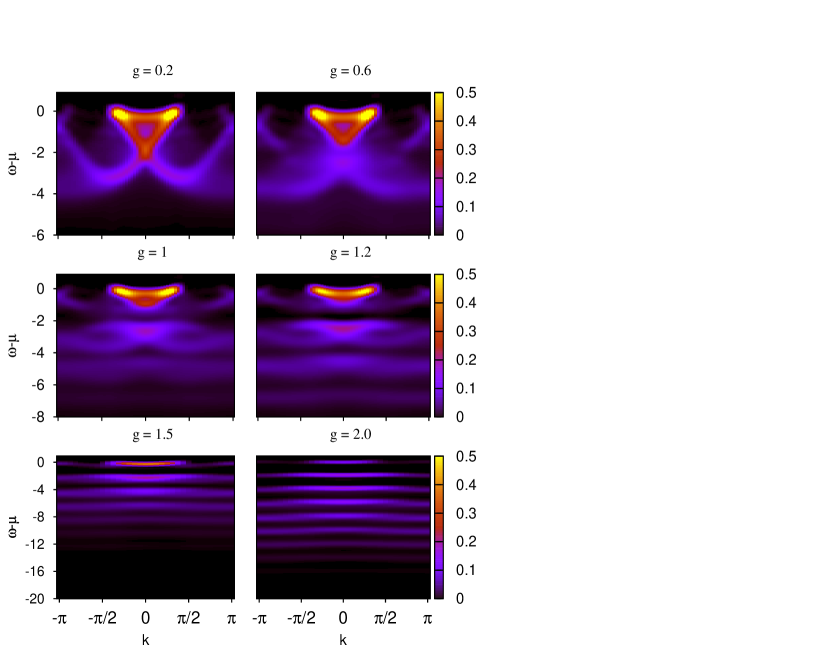
Figure 1: Photoemission spectrum of the HH model calculated with tDMRG in the antiadiabatic regime ($\omega_{0}=2.0$) for different e-ph couplings $g=0.2,0.6,1.0,1.2,1.5,2.0$. Here $L=32$ sites, U=20 and filling N/L=3/4.

Figure 2: Three cuts at $k=0,k_{F},2k_{F}$ of photoemission spectrum shown in Fig.1.

IV tDMRG RESULTS

The properties of the PES are analyzed starting from ($\omega_{0}>1$) and considering in particular $\omega_{0}=2.0$. In this regime, Fig.1 shows $B(k,\omega)$ from weak e-ph coupling $g=0.2$ up to strong interaction $g=2.0$.

In order to interpret the results in more detail, Fig.2 is showing three vertical cuts at $k=0$, $k=k_{F}$ ($k_{F}=\pi N/2L=0.375\pi$), and $k=2k_{F}$ of the same spectrum. We note that the spectrum for $g=0.2$ is very similar to the $g=0$ PES (not shown): it is very clear the presence of SCS, where the spectral weight concentrated on the spinon and holon bands forming a triangular spectral structure between $-k_{F}$ and $+k_{F}$ (Fig.1). As expected for a Luttinger liquid, the shadow bands extend beyond $k_{F}$. A closer look at PES in Fig.2 in this weak coupling regime, shows that for $k=k_{F}$ and $k=0$ phonon effects are negligible: one can observe clearly the higher spinon peak at the top of the spectrum (at $\omega-\mu\simeq-0.05$ for $k=k_{F}$), and a shifted holon peak. The e-ph effects are already present at this weak coupling for $k=2k_{F}$, where a shoulder on the left of the main peak correspondent to the shadow band is visible.

For $g=0.6$, phonon effects come already into play with very interesting features at all momenta. Looking at Fig.1, one can observe a reduction of the spinon and holon bandwidth, as the triangular spectral structure comprising the spinon and holon bands gets squeezed. An apparent suppression of the spectral weight or gap seems to appear at $\omega-\mu\simeq-2$ with the formation of a new band ranging from $\omega-\mu\simeq-2$ to $\omega-\mu\simeq-4$, whose dispersion resembles those of the holon and shadow bands. The same characteristics are visible in Fig.2 for $k=0$, where the distance between the spinon peak and the holon peak is reduced and a side-band at the left of the holon peak is formed. This new spectral feature seems to originate from the holon band, while the height of the spinon peak is practically unchanged going from $g=0.2$ to $g=0.6$.

At $g=1.0$, the progressive reduction of the electronic bandwidth (both of the spinon and holon bands) is even more evident, and the triangular spectral structure has almost collapsed. The new band formed at $g=0.6$ is now separated by a larger gap with respect to the main spectrum, while the spectral redistribution creates now a newer side-band whose width is smaller and ranging from $\omega-\mu\simeq-4$ to $\omega-\mu\simeq-6.2$. As one can see, in Fig.2 for $k=0$, several side-bands separated in energy by a quantity proportional to $\omega_{0}$ are visible. The side-bands present no internal structure and suggest that, up to $g=1.0$, they originate from the holon bands without contribution from the spinons.

For $g=1.2$, the original triangular feature in the PES is completely collapsed to a flat structure. Also, if one looks at Fig.2 for $k=0$ and $k=k_{F}$ for the same value of $g$, the height of the first spectral peak is dramatically increased with respect to the case of $g=1.0$. This indicates that one is entered in the strong e-ph coupling regime where the main band is followed by many side-bands coming from both holon and spinon bands. This description, as one can see in Fig.1, is even more evident for $g=1.5$, where the PES is broken in spectral lines whose weight decreases from the first structure to the followings and extends beyond the Fermi momentum $k_{F}$. Besides, the separation between the holon and the spinon peak is not discernible anymore, suggesting that the system is going towards a state that can be described in terms of a spinless polaronic liquid where the spins are completely uncorrelated. Indeed, for $g=2.0$, the physics of phonon side-bands is dominating the PES, observing that the several spectral structures have a smaller width (compared to $g=1.5$ results), bigger height, and that the first spectral structure has less weight than the second one. This is reproducing approximatively a transition to a Gaussian distribution of the spectral weights typical of the polaronic regime.

In order to investigate further this behavior, we have studied the ground state density distribution function in momentum space $n_{k}=(1/L)\sum_{i},je^{-ik(i-j)}\langle c^{\dagger}_{i}c_{j}\rangle$ and the spin-spin correlation function in real space, $\langle S_{z}(L/2)S_{z}(L/2+i)\rangle$. As expected for correlated 1D systems, the density distribution function in momentum space shown in Fig.3 presents a smooth decrease at the Fermi momentum $k_{F}$ for all e-ph coupling values. We point out that the e-ph coupling reduces the decrease at $k_{F}$ and, globally, it broadens the density distribution function. Eventually, for $g=2.0$, one gets a Gaussian profile with $n_{k=0}\simeq 0.45$ and $n_{k=\pi}\simeq 0.325$. In Panel(b) of Fig.3, the spin-spin correlation function from the center of the chain is shown. Up to $g=1.5$, spin-spin correlations fast decay as a function of the distance from the center of the chain with approximately the same behavior. For $g=2.0$, they decay even faster, showing evidence that, in the polaronic regime spin degrees of freedom are completely uncorrelated.

In order to get a better interpretation of the aforementioned results, in the next section an analytical approach for calculating the PES will be introduced, explaining the redistribution of the spectral weight in terms of phonon side-bands.

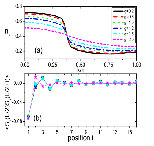
Figure 3: Panel(a) Density distribution function in momentum space for the same parameter values as in Fig.1. Solid (black), dashed (red) dotted (green), dashed-dotted (blue), dashed-dotted-dashed (cyan), short-dashed (magenta), represent respectively $g=0.2,0.6,1.0,1.2,1.5,2.0$. Panel (b) Spin-spin correlation function from the center of the chain for the same parameter values as Panel (a).

V ANALYTICAL APPROACH

In this section we present an analytical method that allows us to calculate the photoemission part of the spectral function

$$B(k,\omega)=-\frac{1}{\pi}ImG(k,\omega)\mspace{30.0mu}for\mspace{10.0mu}\omega<\mu,$$ (4)

where $G(k,\omega)$ is the electronic retarded single particle Green’s function and $\mu$ is the chemical potential. The method consists of a variational canonical transformation originally proposed in Ref.Zheng et al., 1989 (we refer to it as the ZFA approach, from the paper of Zheng, Feinberg and Avignon) and then employed in Ref.Perroni et al., 2003 for calculating the spectral and optical properties of the spinless Holstein model. The starting point of the approach is the assumption that, in the limit of strong e-ph coupling, $U\rightarrow\infty$ and infinite phonon frequency $\omega_{0}$, the model is described by spinless polarons. The ZFA approach, then, extends the polaron formation to the intermediate e-ph coupling regime, recovering the mean field solution at zero phonon frequency. The generator of the variational Lang-Firsov transformationLang and Firsov (1963) is given by

$$T[f,\Delta]=e^{g\sum\limits_{j}[n_{j}f+\Delta](a_{j}-a^{\dagger}_{j})},$$ (5)

where $f$ and $\Delta$ are variational parameters. The quantity $f$ governs the magnitude of the antiadiabatic polaronic effect, while $\Delta$ represents the lattice distortion proportional to the average electron density. The transformed Hamiltonian is

$$\tilde{H}[f,\Delta]=T^{-1}HT=-t\sum\limits_{<i,j>,\sigma}(c^{\dagger}_{i,\sigma}X^{\dagger}_{i}X_{j}c_{j,\sigma}+h.c.)$$

$$+(U-2g^{2}f^{2}\omega_{0})\sum\limits_{i}n_{i,\sigma}n_{i,\bar{\sigma}}+\omega_{0}\sum\limits_{i}a^{\dagger}_{i}a_{i}+Lg^{2}\omega_{0}\Delta^{2}$$

$$+g\omega_{0}(1-f)\sum\limits_{i}n_{i}(a_{i}+a^{\dagger}_{i})-g\omega_{0}\Delta\sum\limits_{i}(a_{i}+a^{\dagger}_{i})$$

$$+\tilde{\eta}\sum\limits_{i}n_{i},$$ (6)

where $L$ is the total number of lattice sites. Here we have defined a phonon operator $X_{i}=e^{gf(a_{i}-a^{\dagger}_{i})}$ and $\tilde{\eta}=g^{2}\omega_{0}f(f-2)+2g^{2}\omega_{0}(f-1)\Delta$. We leave the technical details of the determination of the variational parameters $f$ and $\Delta$ in the Appendix A. Also, it can be shown easily that the variational parameter $\Delta$ can be obtained as a function of $f$ ($\Delta=(1-f)N/L$), and one is thus left with only one variational parameter. Once the optimal $\tilde{f}$ is determined, one can write the transformed Hamiltonian as

$$\tilde{H}[\tilde{f}]=\tilde{H}_{0}+V,$$ (7)

where $\tilde{H}_{0}$ is the unperturbed part given by strongly correlated electrons and non-interacting phonons,

$$\tilde{H}_{0}[\tilde{f}]=-te^{-g^{2}\tilde{f}^{2}}\sum\limits_{<i,j>,\sigma}(c^{\dagger}_{i,\sigma}c_{j,\sigma}+h.c.)$$

$$+(U-2g^{2}\tilde{f}^{2}\omega_{0})\sum\limits_{i}n_{i,\sigma}n_{i,\bar{\sigma}}+\omega_{0}\sum\limits_{i}a^{\dagger}_{i}a_{i}+\eta N$$

$$-g\omega_{0}(1-\tilde{f})\frac{N}{L}\sum\limits_{i}(a_{i}+a^{\dagger}_{i})+g^{2}\omega_{0}(1-\tilde{f})^{2}\frac{N^{2}}{L},$$

with $\eta=g^{2}\omega_{0}\tilde{f}(\tilde{f}-2)-2g^{2}\omega_{0}(1-\tilde{f})^{2}N/L$, while $V$ is a many-body interaction

$$V = -t\sum\limits_{<i,j>,\sigma}[c^{\dagger}_{i,\sigma}(X^{\dagger}_{i}X_{j}-e^{-g^{2}\tilde{f}^{2}})c_{j,\sigma}+h.c.]$$

$$+g\omega_{0}(1-\tilde{f})\sum\limits_{i}n_{i}(a_{i}+a^{\dagger}_{i}).$$

The PES is now calculated approximately by neglecting the perturbation $V$. One can use perturbation theory and consider the effect of $V$ in higher orders of perturbation after the calculation of the PES, but in this paper we are only taking the zeroth order into account. In fact, the determination of the optimal parameter $\tilde{f}$ is meant to minimize the error produced by neglecting the interaction term $V$ from the Hamiltonian Eq.(7). The unperturbed Hamiltonian $\tilde{H}_{0}[\tilde{f}]$ still contains information about interacting terms in the original Hamiltonian Eq.(1), since all the parameters of $\tilde{H}_{0}[\tilde{f}]$ are renormalized by our variational technique. Indeed, $\tilde{H}_{0}[\tilde{f}]$ consists of free phonons and a Hubbard model with a hopping $\tilde{t}$ and an on-site repulsion $\tilde{U}$ renormalized by the e-ph interaction

$$\tilde{t}=te^{-g^{2}\tilde{f}^{2}},\tilde{U}=U-2g^{2}\tilde{f}^{2}\omega_{0}.$$ (10)

The PES is now evaluated in the Lehmann representation

$$B(k,\omega) = \sum_{\{n_{ph}\},z,\sigma}|\langle|\{n_{ph}\},z,N-1|c_{k,\sigma}|\{0_{ph}\},gs,N\rangle|^{2}$$ (11)

$$\times L\delta(\omega-E_{gs}^{N}+E_{z}^{N-1}),$$

where $c_{k,\sigma}$ destroys an electron with momentum $k$ and spin $\sigma$ ($c_{j,{\sigma}}=\frac{1}{\sqrt{L}}\sum_{k^{\prime}}e^{ik^{\prime}j}c_{k^{\prime},\sigma}$), $N$ is the total number of electrons, and $z$ the final state with $N-1$ electrons. $E_{z}^{N-1}$ represents the total energy of the final state, $|\{n_{ph}\},z,N-1\rangle$, where a generic phonon contribution is included, and $E_{gs}^{N}$ describes the energy of the ground state of the original Hamiltonian (1) with $N$ electrons. Since Einstein phonons carry no momentum, we can impose the momentum conservation with the term $\delta_{k,P_{gs}^{N}-P_{z}^{N-1}}$ to reduce Eq.(11) to a calculation involving only site $0$ in the real space and one phonon mode at that site

$$B(k,\omega) = \sum_{\{n_{ph}\},z,\sigma}|\langle|\{n_{ph}\},z,N-1|c_{0,\sigma}|\{0_{ph}\},gs,N\rangle|^{2}$$ (12)

$$\times L\delta(\omega-E_{gs}^{N}+E_{z}^{N-1})\delta_{k,P_{gs}^{N}-P_{z}^{N-1}}.$$

Up to here, no assumptions have been made on the spectral function and this general form is extremely complex. However, in the basis of $\tilde{H_{0}}$, the wave-function is trivially separated into phonon and electronic parts. In the limit of $\tilde{U}>>\tilde{t}$ one can use Ogata-Shiba’s factorizationOgata and Shiba (1990) to show that the electronic wave-function itself is split into spin and charge parts. The total wave-function can be written as

$$|\mathrm{\psi}\rangle=|\phi\rangle\otimes|\chi\rangle\otimes|\{n_{ph}\}\rangle.$$ (13)

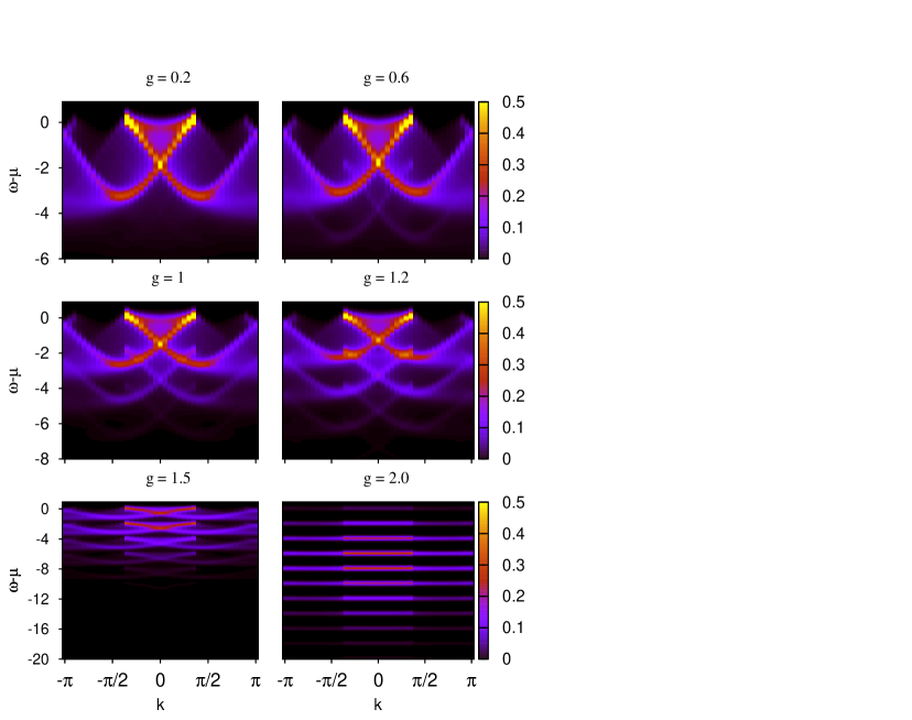
Figure 4: (Color online) Photoemission spectrum calculated with analytical method for the same frequency and e-ph coupling values considered in Fig.1. Here $L=40$ sites, $U=20$ and filling $N/L=3/4$.

The first part, $|\phi\rangle$, describes spinless charges, $|\chi\rangle$ is the spin wave-function that corresponds to a “squeezed” chain of $N$ spins, where all the unoccupied sites have been removed, and $|\{n_{ph}\}\rangle$ is given by the product of $L$ separate non-interacting phononic wave-functions, each one containing an integer number of phonons $(|\{n_{ph}\}\rangle=|\{n_{ph}^{0}\}\rangle\otimes|\{n_{ph}^{1}\}\rangle\otimes...|\{n_{ph}^{L-1}\}\rangle).$ In this limit, charge, spin, and lattice degrees of freedom are governed by independent Hamiltonians

$$\tilde{H}_{0}[\tilde{f}]=\tilde{H}_{charge}+\tilde{H}_{spin}+\tilde{H}_{phonon}.$$ (14)

Due to this simplification, we are now able to tackle the problem and calculate the PES. Indeed, operator $c_{0,\sigma}$ after the polaron transformation will look like $c_{0,\sigma}X_{0}$. Moreover, by using the factorized wave-function and separating spin and charge operators, $c_{0,\sigma}X_{0}=Z_{0,\sigma}b_{0}X_{0}$, the spectral function can be expressed as a convolution

$$B(k,\omega)=\sum\limits_{\omega^{\prime},Q,\sigma}D_{\sigma}(Q,\omega^{\prime})B_{Q}(k,\omega-\omega^{\prime})$$ (15)

where $D_{\sigma}(Q,\omega)$ is the spin spectral function with momentum $Q$, and

$$B_{Q}(k,\omega)=L\sum\limits_{\{I\}}\{|\langle\psi_{L,Q}^{N-1}\{I\}|b_{0}|\psi_{L,\pi}^{N,gs}\rangle|^{2}$$

$$\times \sum\limits_{\tilde{n}}|\langle\tilde{n}|X_{0}|0\rangle|^{2}\delta(\omega-E^{N}_{gs}+E^{N-1}_{z}+\tilde{n}\omega_{0})$$

$$\delta_{k,P^{N}-P^{N-1}}\},$$

describes the charge and phonon parts. By following the approach introduced in Ref.Penc et al., 1997, one can calculate numerically both $D_{\sigma}(Q,\omega)$ and $B_{Q}(k,\omega)$.

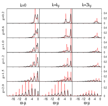
Figure 5: Three cuts at $k=0,k_{F},2k_{F}$ of photoemission spectrum calculated with the tDMRG (solid (black) line, shown also in Fig.2) and using the ZFA approach (dashed (red) line).

Fig.4 shows the PES calculated with the ZFA approach in the antiadiabatic regime, for the same regime of parameters of Fig.1. In analogy with the tDMRG results, we also show three vertical cuts of the spectrum at $k=0$, $k=k_{F}$, $k=2k_{F}$ in Fig.5 (dashed (red) line). It is important to point out that, even within the ZFA approach, a broadening of the spectral peaks of the order of $\delta\simeq 0.25$ has been used.

As stated at the beginning of this section, one expects that the ZFA approach is a good approximation of the results in the regime where $\tilde{U}>>\tilde{t}$ and $\omega_{0}>\tilde{t}$. Also, the optimized polaronic parameter $\tilde{f}$ (see Appendix A) is describing the degree of polaron formation, that is the amount of spectral weight redistribution in phonon side-bands. In general, for $\tilde{f}=1$ one has well defined polarons, while, for $\tilde{f}=0$, the unitary transformation, Eq.5, becomes trivially the identity. As one can observe in Fig.7 (Appendix A), for the set of parameters used in this paper, $U=20$ and $\omega_{0}=2.0$, $\tilde{f}$ assumes a value of $0.4$ for $g=0.2$ increasing slightly up to $0.5$ for $g=1.2$, pointing out that strong Coulomb repulsion and the large phonon frequency already give a sizeable effect from weak to intermediate e-ph couplings. In particular, as one can see in the top row of panels of Fig.2, for $g=0.2$ a very good agreement between ZFA and the tDMRG results is obtained. This characteristic is also evident at all momenta if one looks at the upper left panel of Fig.1 and Fig.4.

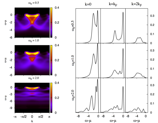
Figure 6: Panel(a) Photoemission spectrum at e-ph couplings $g=1.0$, for different phonon frequencies $\omega_{0}=0.5,1.0,2.0$. Panel(b) Cut at $k=0$, $k=k_{F}$, and $k=2k_{F}$ of photoemission spectrum reported in Panel (a).

Noticeable differences between the ZFA approach and the tDMRG results can be observed in the intermediate e-ph coupling regime ($g=0.6,1.0,1.2$). In this case, the ZFA approach is qualitatively reproducing the reduction of the spinon and holon bandwidths, which are parametrized by the renormalized hopping parameter $\tilde{t}=te^{-g^{2}{\tilde{f}}^{2}}$ in the Hamiltonian $H_{0}[\tilde{f}]$, Eq.(7). Moreover, while reproducing correctly the spectral position of the phonon side-bands, the ZFA approach provides access to their internal structure, showing that the separation between the holon and spinon peaks is still well defined.

At strong e-ph coupling, one has $\tilde{f}=0.675$ for $g=1.5$ and $\tilde{f}=0.975$ for $g=2.0$, observing a large polaronic effect. In these cases, the PES calculated within the ZFA approach provides the same number of phonon side bands with widths and heights of the same order of magnitude of the tDMRG results. As in the tDMRG, the internal structure of the phonon side-bands is lost, while a clear Gaussian-like distribution of the spectral weight is observable for $g=2.0$. Strikingly, the ZFA approach is giving qualitatively the same non-zero spectral weight distribution at momenta larger than $k_{F}$, confirming that, in this case, the system can be described as a polaron liquid. It is important to observe finally that our analytical approach provides a shift of the chemical potential given by the quantity ${\tilde{\eta}}=g^{2}\omega_{0}{\tilde{f}}({\tilde{f}}-2)+2g^{2}\omega_{0}({\tilde{f}}-1)\Delta$. The optimal shift is in total agreement with tDMRG results in the whole range of e-ph couplings.

We can now briefly discuss the results described above making a contact with the experiments described in Ref.Lee et al., 2013. In this paper, the authors measure the RIXS spectra of a family quasi 1D cuprates $Ca_{2+5x}Y_{2-5x}Cu_{5}O_{10}$, an insulating system that can be doped over a wide range of hole concentrations. The experiment reveals a $70$ meV phonon (energy larger than the typical transfer hopping $t$ along chains in quasi 1-D cuprates) strongly coupled to the electronic state at different hole dopings. It is found that the spectral weight of phonon excitations in the RIXS spectrum is directly dependent on the e-ph coupling strength and doping, producing multiple peaks in the spectrum with an energy separation corresponding to the energy of the quanta of the lattice vibrations, in a fashion similar to what we obtain in the present paper. We believe that, even in ARPES spectra of these materials, phonon side-bands structures in the PES could be observable.

VI tDMRG RESULTS FOR INTERMEDIATE e-ph COUPLING

In this section, we extend the analysis by discussing tDMRG results for intermediate e-ph coupling $g=1.0$, as a function of the phonon frequency $\omega_{0}$. The results are shown in Fig.6. For $\omega_{0}=0.5$, we observe a behavior different from that discussed in the previous section. For instance, at $k=0$, a dip structure at the left side of the spinon peak is shifted by a quantity equal to $\omega_{0}=0.5$, reproducing qualitatively the results discussed in Ref.Matsueda et al., 2006. In Ref.Matsueda et al., 2006, the interpretation of results starts from the consideration that, in absence of e-ph coupling, according to the Bethe ansatz solution the PES is constructed by a superposition of a set of holon dispersions forming a cosine band with width $4t$. Moreover, each holon dispersion is characterized by one spinon momentum. In the presence of e-ph interaction, due to spin-charge separation each holon couples with phonons independently and the PES is interpreted as a spectrum of spinless electron dressed by Einstein phonons. This generates a split of the holon dispersion that is away from the top of the spectrum by a energy interval equal to $\omega_{0}$, and a transfer of spectral weight to high energy giving a characteristic peak-dip-hump structure. Our results are consistent with this picture, confirming that spin-charge separation is robust in this regime. Actually, in contrast to what discussed in the previous section for $\omega_{0}=2.0$, where polaronic effects dominate, when the phonon frequency is smaller than the hopping $t$, the e-ph coupling effect gives rise to a dip in between the holon and spinon peak. Moreover, this spectral dip structure is furthermore shifted if $\omega_{0}$ is increased to $\omega_{0}=1.0$ (See panel(b) of Fig.6 for $\omega_{0}=1.0$ and $k=0$). In this case, our data shows also a shoulder on the left side of the holon peak, in contrast to what found in Ref.Matsueda et al., 2006. In our calculation, this feature can be interpreted as the onset of phonon side-bands. Increasing the phonon frequency to $\omega_{0}=2.0$, several sidebands in the PES are found as discussed in the previous section. Interestingly, at $k=k_{F}$, instead of a dip, we find a peak separated from the spinon band by a energy distance equal to $\omega_{0}$. Eventually, at the Fermi momentum and for larger frequencies, these features become part of the first and the higher side-bands.

VII CONCLUSION

We have studied the spectral function of the 1D HH model using the tDMRG, in the limit of large Coulomb repulsion, and away from electronic half-filling. The entire range of e-ph coupling, from weak to strong coupling $g$, has been analyzed. Our results indicate that, from weak to intermediate $g$, SCS is robust against e-ph coupling: the phonons couple mainly with charge degrees of freedom, leaving the spinon band almost unaffected. For sufficiently strong e-ph interaction, the PES weight is redistributed in phonon side-bands, and the spinon and holon spectral features are not discernable anymore. In this regime, we support the numerical tDMRG results with an analytical variational calculation, approximating the wave-function as a convolution of charge, spin and phonon parts. In this case, a very good qualitative and quantitative agreement is obtained, and the system can be described as a polaronic liquid, with non-zero spectral weight at momenta larger than the Fermi momentum.

VIII ACKNOWLEDGMENTS

A.E.F. acknowledges NSF support through grant DMR-1339564. A. N. thanks Lev Vidmar for useful comments.

Appendix A VARIATIONAL CALCULATION OF THE PARAMETER $f$

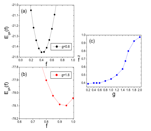
Figure 7: Panels (a) and (b) The ground-state energy as a function of $f$ in order to get $\tilde{f}$. Panel (c) $\tilde{f}$ as a function of $g$ for filling N/L=0.75

In this appendix we determine the variational parameters $f$ and $\Delta$ appearing in the transformed Hamiltonian Eq.(6) of the main text. An effective electronic Hamiltonian, $H_{eff}$, is used, which is obtained by averaging Eq.(6) on the phononic vacuum of the transformed Hilbert space, $H_{eff}[f,\Delta]=\langle O_{ph}|\tilde{H}|O_{ph}\rangle$

$$H_{eff}[f,\Delta]=-te^{-g^{2}f^{2}}\sum\limits_{<i,j>,\sigma}(c^{\dagger}_{i,\sigma}c_{j,\sigma}+h.c.)$$ (17)

$$+(U-2g^{2}f^{2}\omega_{0})\sum\limits_{i}n_{i,\sigma}n_{i,\bar{\sigma}}+\eta\sum\limits_{i}n_{i}+Lg^{2}\omega_{0}\Delta^{2}.$$

The parameter $\Delta$ is simply obtained by using the Hellmann-Feynman theorem

$$\frac{\partial}{\partial\Delta}\langle gs|H_{eff}|gs\rangle=0\Rightarrow\Delta=(1-f)\frac{N}{L},$$

where $N$ is the total number of electrons, $N/L$ is the electronic density, and $|gs\rangle$ is the ground state of $H_{eff}$. Now we are left only with the determination of the parameter $f$, which will be found by solving the Hamiltonian

$$H_{eff}[f]=-te^{-g^{2}f^{2}}\sum\limits_{<i,j>,\sigma}(c^{\dagger}_{i,\sigma}c_{j,\sigma}+h.c.)$$ (18)

$$+(U-2g^{2}f^{2}\omega_{0})\sum\limits_{i}n_{i,\sigma}n_{i,\bar{\sigma}}+g^{2}\omega_{0}(1-f)^{2}N^{2}/L+\eta N,$$

by using the static DMRG and minimizing the ground-state energy of this new Hamiltonian $H_{eff}$ as a function of $f$. For each set of values $U$, $t$, $g$, and $\omega_{0}$, considered in the original Hamiltonian, we get an optimal polaronic parameter $\tilde{f}$. In the panels (a) and (b) of Fig.7, the ground-state energy of $H_{eff}[f]$ as a function of $f$ for two different values of e-ph coupling $g=0.8$ and $g=1.8$, $N/L=0.75$, and $\omega_{0}=2.0$ is shown. For $g=1.8$ the value of $\tilde{f}$ obtained is close to $0.8$ meaning that for these sets of parameters the system is near the polaronic regime, that ideally is expected to be reached for stronger e-ph coupling and phonon frequency. In panel (c) of Fig.7, the optimal polaronic parameter $\tilde{f}$ as a function of e-ph is shown as discussed in the main text.

References

- Lanzara et al. (2001) A. Lanzara, P. Bogdanov, X. Zhou, S. Kellar, D. Feng, E. Lu, T. Yoshida, H. Eisaki, A. Fujimori, K. Kishio, et al., Nature 412, 510 (2001).
- Gweon et al. (2004) G.-H. Gweon, T. Sasagawa, S. Zhou, J. Graf, H. Takagi, D.-H. Lee, and A. Lanzara, Nature 430, 187 (2004).
- Gunnarsson (1997) O. Gunnarsson, Rev. Mod. Phys. 69, 575 (1997).
- Lanzara et al. (1998) A. Lanzara, N. Saini, M. Brunelli, F. Natali, A. Bianconi, P. Radaelli, and S.-W. Cheong, Phys. Rev. Lett. 81, 878 (1998).
- Gogolin et al. (2004) A. O. Gogolin, A. A. Nersesyan, and A. M. Tsvelik, Bosonization and strongly correlated systems (Cambridge University Press, 2004).
- Giamarchi (2004) T. Giamarchi, Quantum Physics in One Dimension (Clarendon Press, Oxford, 2004).
- Deshpande et al. (2010) V. V. Deshpande, M. Bockrath, L. I. Glazman, and A. Yacoby, Nature 464, 209 (2010).
- Auslaender et al. (2005) O. Auslaender, H. Steinberg, A. Yacoby, Y. Tserkovnyak, B. Halperin, K. Baldwin, L. Pfeiffer, and K. West, Science 308, 88 (2005).
- Lorenz et al. (2002) T. Lorenz, M. Hofmann, M. Grüninger, A. Freimuth, G. Uhrig, M. Dumm, and M. Dressel, Nature 418, 614 (2002).
- Bockrath et al. (1999) M. Bockrath, D. H. Cobden, J. Lu, A. G. Rinzler, R. E. Smalley, L. Balents, and P. L. McEuen, Nature 397, 598 (1999).
- Blumenstein et al. (2011) C. Blumenstein, J. Schäfer, S. Mietke, S. Meyer, A. Dollinger, M. Lochner, X. Cui, L. Patthey, R. Matzdorf, and R. Claessen, Nature Physics 7, 776 (2011).
- Kollath et al. (2005) C. Kollath, U. Schollwöck, and W. Zwerger, Physical review letters 95, 176401 (2005).
- Kollath and Schollwöck (2006) C. Kollath and U. Schollwöck, New Journal of Physics 8, 220 (2006).
- Feiguin and Huse (2009) A. E. Feiguin and D. A. Huse, Phys. Rev. B 79, 100507 (2009).
- Kim et al. (2006) B. Kim, H. Koh, E. Rotenberg, S.-J. Oh, H. Eisaki, N. Motoyama, S. Uchida, T. Tohyama, S. Maekawa, Z.-X. Shen, et al., Nature Physics 2, 397 (2006).
- Sing et al. (2003) M. Sing, U. Schwingenschlögl, R. Claessen, P. Blaha, J. Carmelo, L. Martelo, P. Sacramento, M. Dressel, and C. S. Jacobsen, Physical Review B 68, 125111 (2003).
- Lee et al. (2013) W. S. Lee, S. Johnston, B. Moritz, J. Lee, M. Yi, K. J. Zhou, T. Schmitt, L. Patthey, V. Strocov, K. Kudo, et al., Phys. Rev. Lett. 110, 265502 (2013).
- Lee et al. (2014) J. J. Lee, B. Moritz, W. S. Lee, M. Yi, C. J. Jia, A. P. Sorini, K. Kudo, Y. Koike, K. J. Zhou, C. Monney, et al., Phys. Rev. B 89, 041104 (2014).
- Matsueda et al. (2006) H. Matsueda, T. Tohyama, and S. Maekawa, Physical Review B 74, 241103 (2006).
- Ning et al. (2006) W.-Q. Ning, H. Zhao, C.-Q. Wu, and H.-Q. Lin, Physical review letters 96, 156402 (2006).
- White and Feiguin (2004) S. R. White and A. E. Feiguin, Phys. Rev. Lett. 93, 076401 (2004).
- Daley et al. (2004) A. J. Daley, C. Kollath, U. Schollwock, and G. Vidal, Journal of Statistical Mechanics: Theory and Experiment 2004, P04005 (2004).
- Hardikar and Clay (2007) R. P. Hardikar and R. T. Clay, Phys. Rev. B 75, 245103 (2007).
- Ogata and Shiba (1990) M. Ogata and H. Shiba, Physical Review B 41, 2326 (1990).
- Reja et al. (2011) S. Reja, S. Yarlagadda, and P. B. Littlewood, Phys. Rev. B 84, 085127 (2011).
- Reja et al. (2012) S. Reja, S. Yarlagadda, and P. B. Littlewood, Phys. Rev. B 86, 045110 (2012).
- Perroni et al. (2005) C. A. Perroni, V. Cataudella, G. De Filippis, and V. M. Ramaglia, Phys. Rev. B 71, 113107 (2005).
- Hohenadler and Assaad (2013) M. Hohenadler and F. F. Assaad, Phys. Rev. B 87, 075149 (2013).
- Payeur and Sénéchal (2011) A. Payeur and D. Sénéchal, Phys. Rev. B 83, 033104 (2011).
- Nowadnick et al. (2012) E. A. Nowadnick, S. Johnston, B. Moritz, R. T. Scalettar, and T. P. Devereaux, Phys. Rev. Lett. 109, 246404 (2012).
- Bauer (2010) J. Bauer, EPL (Europhysics Letters) 90, 27002 (2010).
- Bauer and Hewson (2010) J. Bauer and A. C. Hewson, Phys. Rev. B 81, 235113 (2010).
- Kumar and van den Brink (2008) S. Kumar and J. van den Brink, Phys. Rev. B 78, 155123 (2008).
- Barone et al. (2008) P. Barone, R. Raimondi, M. Capone, C. Castellani, and M. Fabrizio, Phys. Rev. B 77, 235115 (2008).
- Fehske et al. (2008) H. Fehske, G. Hager, and E. Jeckelmann, EPL (Europhysics Letters) 84, 57001 (2008).
- Tezuka et al. (2007) M. Tezuka, R. Arita, and H. Aoki, Phys. Rev. B 76, 155114 (2007).
- Ejima and Fehske (2010) S. Ejima and H. Fehske, Journal of Physics: Conference Series 200, 012031 (2010).
- Ejima and Fehske (2009) S. Ejima and H. Fehske, EPL (Europhysics Letters) 87, 27001 (2009).
- Jeckelmann and White (1998) E. Jeckelmann and S. R. White, Phys. Rev. B 57, 6376 (1998).
- Zhang et al. (1999) C. Zhang, E. Jeckelmann, and S. R. White, Phys. Rev. B 60, 14092 (1999).
- Cataudella et al. (2004) V. Cataudella, G. De Filippis, F. Martone, and C. A. Perroni, Phys. Rev. B 70, 193105 (2004).
- Manmana et al. (2005) S. R. Manmana, A. Muramatsu, and R. M. Noack, AIP Conference Proceedings 789 (2005).
- Schmitteckert (2004) P. Schmitteckert, Phys. Rev. B 70, 121302 (2004).
- Cazalilla and Marston (2002) M. Cazalilla and J. Marston, Physical review letters 88, 256403 (2002).
- Cazalilla and Marston (2003) M. Cazalilla and J. Marston, Physical Review Letters 91, 049702 (2003).
- Luo et al. (2003) H. Luo, T. Xiang, and X. Wang, Physical review letters 91, 49701 (2003).
- Zheng et al. (1989) H. Zheng, D. Feinberg, and M. Avignon, Phys. Rev. B 39, 9405 (1989).
- Perroni et al. (2003) C. A. Perroni, V. Cataudella, G. De Filippis, G. Iadonisi, V. Marigliano Ramaglia, and F. Ventriglia, Phys. Rev. B 67, 214301 (2003).
- Lang and Firsov (1963) I. J. Lang and Y. A. Firsov, Sov. Phys. JETP 16, 1301 (1963).
- Penc et al. (1997) K. Penc, K. Hallberg, F. Mila, and H. Shiba, Phys. Rev. B 55, 15475 (1997).