Energy transfer and dissipation in forced isotropic turbulence

Abstract

A model for the Reynolds number dependence of the dimensionless dissipation rate $C_{\varepsilon}$ was derived from the dimensionless Kármán-Howarth equation, resulting in $C_{\varepsilon}=C_{\varepsilon,\infty}+C/R_{L}+O(1/R_{L}^{2})$, where $R_{L}$ is the integral scale Reynolds number. The coefficients $C$ and $C_{\varepsilon,\infty}$ arise from asymptotic expansions of the dimensionless second- and third-order structure functions. This theoretical work was supplemented by direct numerical simulations (DNSs) of forced isotropic turbulence for integral scale Reynolds numbers up to $R_{L}=5875$ ($R_{\lambda}=435$), which were used to establish that the decay of dimensionless dissipation with increasing Reynolds number took the form of a power law $R_{L}^{n}$ with exponent value $n=-1.000\pm 0.009$, and that this decay of $C_{\varepsilon}$ was actually due to the increase in the Taylor surrogate $U^{3}/L$. The model equation was fitted to data from the DNS which resulted in the value $C=18.9\pm 1.3$ and in an asymptotic value for $C_{\varepsilon}$ in the infinite Reynolds number limit of $C_{\varepsilon,\infty}=0.468\pm 0.006$.

I Introduction

In recent years there has been much interest in the fundamentals of turbulent dissipation, as characterized by the mean dissipation rate

$$\varepsilon=\frac{\nu_{0}}{2}\sum_{\alpha,\beta=1}^{3}\left\langle\left(\frac{\partial u_{\alpha}}{\partial x_{\beta}}+\frac{\partial u_{\beta}}{\partial x_{\alpha}}\right)^{2}\right\rangle\ ,$$ (1)

where $\nu_{0}$ is the kinematic viscosity, $u_{\alpha}\equiv u_{\alpha}(\bm{x},t)$ is one component of the velocity field $\bm{u}$, while angle brackets denote an ensemble average. For isotropic turbulence, (1) reduces to

$$\varepsilon=\nu_{0}\sum_{\alpha,\beta=1}^{3}\left\langle\left(\frac{\partial u_{\alpha}}{\partial x_{\beta}}\right)^{2}\right\rangle\ .$$ (2)

This interest has centered on the approximate expression for the dissipation rate $\varepsilon$, which was given by Taylor in 1935 Taylor (1935) as

$$\varepsilon=C_{\varepsilon}U^{3}/L,$$ (3)

where $U$ is the root-mean-square velocity and $L$ is the integral scale. Many workers in the field refer to Eq. (3) as the Taylor dissipation surrogate. However, others re-arrange it to define the coefficient $C_{\varepsilon}$ as the nondimensional dissipation rate; thus,

$$C_{\varepsilon}=\frac{\varepsilon}{U^{3}/L}.$$ (4)

In 1953 Batchelor Batchelor (1971) (we refer to the first edition of this work) presented evidence to suggest that the coefficient $C_{\varepsilon}$ tended to a constant value with increasing Reynolds number. In 1984 Sreenivasan Sreenivasan (1984) showed that in grid turbulence $C_{\varepsilon}$ became constant for Taylor-Reynolds numbers greater than about $50$. He also found a $1/R_{\lambda}$-dependence at low $R_{\lambda}$ and, since at low $R_{\lambda}$ the Taylor-Reynolds number and the integral scale Reynolds number are proportional, Sreenivasan’s paper had already in effect presented empirical evidence for $1/R_{L}$ scaling at low $R_{L}$. We discuss this further, in relation to our present work, in Section IV. Later, in 1998, Sreenivasan presented a survey of investigations of both forced and decaying turbulence Sreenivasan (1998), using direct numerical simulation (DNS), which established the now characteristic curve of $C_{\varepsilon}$ plotted against the Taylor-Reynolds number $R_{\lambda}$ (e.g. see our Fig. 1). More recently, the comprehensive review of dissipation rate scaling by Vassilicos Vassilicos (2015) has summarized the evidence for $1/R_{L}$ scaling of $C_{\varepsilon}$.

In his 1968 lecture notes Saffman (1968), Saffman made two comments about the expression that we have given here as Eq. (3). These were as follows: “This result is fundamental to an understanding of turbulence and yet still lacks theoretical support” and “the possibility that $A$ (i.e. our $C_{\varepsilon}$) depends weakly on the Reynolds number can by no means be completely discounted.” More than 40 yr on, the question implicit in his second comment has been comprehensively answered by the survey papers of Sreenivasan Sreenivasan (1984, 1998), along with a great deal of subsequent work by others, some of which we have cited here. However, while some theoretical work has indicated an inverse proportionality between $C_{\varepsilon}$ and Reynolds number, this has been limited to low Reynolds numbers Sreenivasan (1984) or based on a mean-field approximation Lohse (1994) or restricted to providing an upper bound Doering and Foias (2002). Hence, his first comment is still valid today; and this lack of theoretical support remains an impediment to the development of turbulence phenomenology and hence turbulence theory.

In this article we present two pieces of work. These are as follows.

First we develop a theoretical model of the relationship between the dimensionless dissipation rate and the integral scale Reynolds number. We start from the driven Navier-Stokes equation in wavenumber space and specify the nature of the input term to the energy balance equation in wavenumber space. Then we Fourier transform this in order to derive the energy balance in scale space, that is, the Kármán-Howarth equation with forcing. This provides a basis for the application of our general theory for forced isotropic turbulence to the specific case of our DNS driven by negative damping. It also gives a basis for a later consideration of the universality of our conclusions.

Second, we present the data obtained from DNS for a range of integral scale Reynolds numbers up to $R_{L}=5875$. These results are used to elucidate some aspects of the phenomenon and then to test our theoretical model.

We begin with a short review of the relevant literature.

II Some results from both numerical and experimental investigations

Unless otherwise stated, the cited DNSs used the standard pseudospectral method simulating isotropic turbulence in cubic boxes of length $L_{box}=2\pi$. We report on results for forced isotropic turbulence only. Some of the numerical results mentioned below are shown in Fig. 1 alongside our data.

Jiménez et al. Jiménez et al. (1993) attained Taylor-scale Reynolds numbers up to $R_{\lambda}=170$, with their highest $R_{\lambda}$ simulation extending to $0.3\tau$, where $\tau$ denotes the large eddy turnover time. In view of the short execution time this simulation might still be in a transient state. They achieved dealiasing by a combination of random grid shifts and spherical truncation. The system was forced by using negative viscosity for wavenumbers $k\leqslant 2.5$ maintaining $k_{max}\eta$ and hence $\varepsilon$ constant, where $\eta$ denotes the Kolmogorov dissipation scale. The authors reported an asymptotic value for the dimensionless dissipation rate $C_{\varepsilon,\infty}\simeq 0.7$. The statistics were calculated from five to ten realizations for a short execution time. That is, given the sample rate and the run time, the realizations would have been strongly correlated. Regarding resolution requirements, the authors point out that $k_{max}\eta=1$ is the absolute minimum while $k_{max}\eta=2$ is desirable.

In the work of Wang et al. Wang et al. (1996) the forcing was implemented by maintaining the kinetic energy in the two lowest wavenumber shells constant with an energy spectrum following $k^{-5/3}$. The measured asymptote $C_{\varepsilon,\infty}$ lay in the region $0.42\leqslant C_{\varepsilon,\infty}\leqslant 0.49$. Using the same method without dealiasing, Cao et al. Cao et al. (1999) focused mainly on the statistics of the pressure field, but data is provided in their Table 1 from which $C_{\varepsilon}$ can be calculated. The initial condition was similar to our DNS as $E(k,0)\sim k^{4}\exp(k/k_{0})^{2}$, with $k_{0}\simeq 5$ and the system evolved for ten large eddy turnover times before measurements were taken.

Yeung and Zhou Yeung and Zhou (1997) presented time-averaged results from simulations using a partially dealiased code with stochastic forcing, covering a $R_{\lambda}$ range of $38\leq R_{\lambda}\leq 240$ for about four large-eddy turnover times. The resolution was relatively high as all runs satisfied $k_{max}\eta\geq 1.5$.

A partially dealiased code with stochastic forcing was also used by Donzis et al. Donzis et al. (2005), who simulated flows with Taylor-scale Reynolds number up to $R_{\lambda}=390$. The data points for $C_{\varepsilon}$ at different $R_{\lambda}$ were fitted to the expression $C_{\varepsilon}=A(1+\sqrt{1+(B/R_{\lambda})^{2}})$, with $A\simeq 0.2$ and $B\simeq 92$, leading to an asymptote $C_{\varepsilon,\infty}\simeq 0.4$. We discuss this expression for $C_{\varepsilon}$ in more detail in Sec. III.4.

The investigation by Bos et al. Bos et al. (2007) reported results from DNS, Large Eddy Simulation (LES) and Eddy-Damped, Quasi-Normal Markovian closure (EDQNM) calculations for Reynolds numbers up to $R_{\lambda}=100$ for DNS and $R_{\lambda}=2000$ for EDQNM. The authors tested different initial conditions such as Gaussian-shaped initial energy spectra and the von Kármán spectrum and found no dependence on the choice of initial spectrum once the system had reached a stationary state. However, the transient to a steady state was found to be shorter for a von Kármán spectrum than for Gaussian-shaped initial spectra. They measured $C_{\varepsilon,\infty}\simeq 0.5$ for the asymptote of the dimensionless dissipation rate.

Variations of the initial conditions were also studied by Goto and Vassilicos Goto and Vassilicos (2009), mainly by altering the low wave number behavior and the peak wave number of the initial spectra. The results for $C_{\varepsilon}$ show a dependence on the different low wave number forms of the initial spectra. In contrast, the location of the peak of the initial spectrum had no significant influence on $C_{\varepsilon}$. What is interpreted as a dependence on the form of the initial spectra could actually be due to differences in the forcing method. The system is kept statistically stationary by fixing the magnitude of the velocity field modes for wave numbers smaller than the peak wave number of the initial spectra, which in some cases leads to a very large forcing range. The low wave number form of the initial spectrum is thus maintained during the evolution of the velocity field, such that it is no longer purely a feature of the initial condition but rather a permanent feature imposed by the forcing scheme. The observed dependence of $C_{\varepsilon}$ on the choice of initial energy spectrum could therefore be due to differences in the forcing spectrum instead.

Kaneda et al. Kaneda et al. (2003) conducted the largest DNS of forced isotropic turbulence so far on grids of up to $4096^{3}$ collocation points reaching $R_{\lambda}=1201$ in single precision and $R_{\lambda}=732$ in double precision, both at minimum resolution of $k_{max}\eta=1$. The system was maintained statistically stationary by using negative viscosity for wave numbers $k\leqslant 2.5$ in order to keep the total energy constant. Data were collected from single realizations only, resulting in an asymptotic value for $C_{\varepsilon}$ in the range $0.4\leqslant C_{\varepsilon,\infty}\leqslant 0.5$. The largest $R_{\lambda}$ simulation was only carried out for a short time; thus, this run might still be transient.

The most recent high resolution DNS results for the dimensionless dissipation rate were presented by Yeung et al. Yeung et al. (2012). Four simulations spanning a Taylor-scale Reynolds number range of $140\leqslant R_{\lambda}\leqslant 1000$ on $2048^{3}$ and $4096^{3}$ collocation points were carried out, at resolutions between $1.3\leqslant k_{max}\eta\leqslant 11.2$, resulting in $0.449\leqslant C_{\varepsilon}\leqslant 0.470$. Due to the computational cost incurred by simulations of this size, the execution time in steady state was relatively short and the simulation corresponding to $R_{\lambda}=1000$ was stopped after $3.59\tau$. During the steady state, 20 snapshots were taken to populate the ensemble, so samples were taken every $0.18\tau$. Thus the ensemble consisted of realizations that are statistically correlated. The authors noted that a longer run time would be preferable, but argued that since intense fluctuations in $\varepsilon$ are relatively short lived, ensemble averaging over snapshots close in time will still improve statistics.

In contrast to the various pseudospectral DNSs of incompressible turbulent flows cited here, Pearson et al. Pearson et al. (2004) used a sixth-order finite difference scheme with large-scale $\delta(t)$-correlated forcing for DNS of slightly compressible flows, leading to $C_{\varepsilon}\simeq 0.5$.

Having summarized numerical results on the topic we now briefly turn to experimental results. Pearson et al. Pearson et al. (2002) measured $C_{\varepsilon}\simeq 0.5$ for a number of shear flows. Different flow types were investigated by Burattini et al. Burattini et al. (2005), and Mazellier et al. Mazellier and Vassilicos (2008) studied turbulence in a wind tunnel generated from a variety of different grid geometries including fractal grids. In the fractal case they found a significantly lower asymptote for $C_{\varepsilon}$, namely, $C_{\varepsilon,\infty}\simeq 0.065$. However, we should note that turbulence generated in this way differs in other quite profound ways from conventional grid turbulence.

In all, we find that the asymptotic value $C_{\varepsilon,\infty}\simeq 0.5$ is a well-established numerical result which is broadly in agreement with experimental work.

III A model for the dependence of dimensionless dissipation on Reynolds number

The use of external random forcing with the Navier-Stokes equations (NSEs) was pioneered in the development of statistical theories in the late 1950s. This work was very much influenced by problems in statistical physics, such as Brownian motion, and the emphasis was on choosing forces which could lead to turbulence that was characteristic of the NSE, rather than the forcing. For this reason we begin with a spectral formulation. However, it is also convenient in that it allows us to make a connection with our DNS, which employs the usual pseudospectral method. We obtain the energy balance in wavenumber space (the Lin equation), and then Fourier transform this to obtain the energy balance in scale space. The result is, of course, fully equivalent to the Kármán-Howarth equation with forcing, as derived entirely by more conventional means; see Chap. 4 in the book McComb (2014). In obtaining our theoretical model for the dimensionless dissipation rate, we introduce the dimensionless Kármán-Howarth equation and make asymptotic expansions of the structure functions in inverse powers of the integral scale Reynolds number. We first consider the idealized problem of isotropic turbulence with $\delta-$function forcing in wave number and then apply the analysis to the finite forcing used in the DNS.

III.1 Energy balance and the nature of the forcing

In Fourier space, the incompressible NSEs may be written as:

$$(\partial_{t}+\nu_{0}k^{2})\bm{u}(\bm{k},t) =i\bm{k}P(\bm{k},t)+\int_{\mathbb{R}^{3}}d\bm{j}\ (i\bm{k}\cdot\bm{u}(\bm{j},t))\bm{u}(\bm{k}-\bm{j},t)+\bm{f}(\bm{k},t)\ ,$$

$$i\bm{k}\cdot\bm{u}(\bm{k},t)=0\ ,$$ (5)

where $\bm{u}(\bm{k},t)$ denotes the three-dimensional Fourier transform of the velocity field $\bm{u}(\bm{x},t)$, $P(\bm{k},t)$ the Fourier transform of the pressure field, $\nu_{0}$ the kinematic viscosity, and $\bm{f}(\bm{k},t)$ the Fourier transform of the stirring force $\bm{f}(\bm{x},t)$. In order to avoid introducing unwanted correlations into the problem, the stirring forces must be highly uncorrelated in time. For this reason, they are normally taken to have delta-function autocorrelations in time; see Kraichnan (1959); Edwards (1964); McComb (1990, 2014). In other statistical problems, this input is often referred to as white noise.

The energy balance in wavenumber space (the Lin equation) can readily be derived from the above NSE (see McComb (2014)) to obtain the well known form

$$\frac{\partial E(k,t)}{\partial t}=T(k,t)-2\nu_{0}k^{2}E(k,t)+W(k,t)\ ,$$ (6)

where $E(k,t)$ and $T(k,t)$ are the energy and transfer spectra, respectively, and

$$W(k,t)=4\pi k^{2}\langle\bm{u}(-\bm{k},t)\cdot\bm{f}(\bm{k},t)\rangle$$ (7)

is the work spectrum of the stirring force. For conciseness we do not explicitly show the time dependence from now on.

In order to avoid introducing a dependence on the forcing in wave number space, it was argued by Edwards in 1965 that the forcing spectrum could take the form of a $\delta$-function at the origin. In a modern notation McComb (2014), this may be written as

$$W(k)=\varepsilon_{W}\delta(k),$$ (8)

thus introducing the injection rate $\varepsilon_{W}$ which, in more general terms, is defined by

$$\varepsilon_{W}=\int^{\infty}_{0}W(k)\ dk\ .$$ (9)

At this point we note that $W(k)$ is integrable, which follows from the well posed nature of the problem, as both $\bm{f}$ and $\bm{u}$ should be square-integrable in order to ensure that the total energy remains finite (and to ensure the existence of the respective Fourier transforms).

An alternative to the use of stirring forces exists in the form of negative damping at low wave numbers. This was introduced to theoretical work in 1966 by Herring Herring (1966) and to numerical simulation by Machiels in 1997 Machiels (1997). It is now quite widely used and, as in several of the investigations cited herein, it was used in our present DNS. In this method, the Fourier transform of the force is given by

$$\bm{f}(\bm{k},t) =(\varepsilon_{W}/2E_{f})\bm{u}(\bm{k},t)\quad\text{for}\quad 0<\lvert\bm{k}\rvert<k_{f},$$

$$=0\quad\textrm{otherwise},$$ (10)

$E_{f}$ being the total energy contained in the forcing band. This ensures that the energy injection rate is $\varepsilon_{W}=\textrm{constant}$. The highest forced wavenumber, $k_{f}$, is usually taken to be small. This form of energy input was used in our numerical simulations, as discussed in Section IV.

III.2 The Kármán-Howarth equation for forced turbulence

Now we obtain the equivalent form of the Kármán-Howarth equation (KHE), by Fourier transformation of the Lin equation McComb et al. (2014) as

$$-\frac{3}{2}\frac{\partial U^{2}}{\partial t}+\frac{3}{4}\frac{\partial S_{2}(r)}{\partial t}=-\frac{1}{4r^{4}}\frac{\partial}{\partial r}\Big{(}r^{4}S_{3}(r)\Big{)}+\frac{3\nu_{0}}{2r^{4}}\frac{\partial}{\partial r}\left(r^{4}\frac{\partial S_{2}(r)}{\partial r}\right)-I(r)\ ,$$ (11)

where the longitudinal structure functions are defined as

$$S_{n}(r)=\left\langle\big{(}[\bm{u}(\bm{x}+\bm{r})-\bm{u}(\bm{x})]\cdot\bm{\hat{r}}\big{)}^{n}\right\rangle\ ,$$ (12)

and the input $I(r)$ is given in terms of $W(k)$ by

$$I(r) =3\int_{0}^{\infty}dk\ W(k)\ \left[\frac{\sin{kr}-kr\cos{kr}}{(kr)^{3}}\right]\ ,$$ (13)

where the convergence of this integral is a consequence of the integrability of $W(k)$ ensured by the well posed nature of this problem as stated below (9) in the previous section. Here $I(r)$ is interpreted as the total energy injected into all scales $>r$. Note that we may make the connection between $W(k)$ and the injection rate for the numerical simulations by

$$I(0)=\int^{\infty}_{0}dk\,W(k)=\varepsilon_{W}\ ,$$ (14)

where the energy injection rate $\varepsilon_{W}$ is as specified for the DNS by (10).

It is also helpful to introduce the energy decay rate $\varepsilon_{D}=-(3/2)\partial U^{2}/\partial t$, and with some rearrangement (11) may be written as

$$\varepsilon_{D}=-\frac{3}{4}\frac{\partial S_{2}(r)}{\partial t}-\frac{1}{4r^{4}}\frac{\partial}{\partial r}\Big{(}r^{4}S_{3}(r)\Big{)}+\frac{3\nu_{0}}{2r^{4}}\frac{\partial}{\partial r}\left(r^{4}\frac{\partial S_{2}(r)}{\partial r}\right)-I(r)\ .$$ (15)

At this stage we have a general form of the KHE, but it does not contain the dissipation rate as such (irrespective of how the KHE is derived). As it is the dissipation rate which interests us, we may introduce it to the KHE by a simple identity. This can be derived by integration of the Lin equation (6) with respect to wavenumber. Hence, one obtains for the energy balance of isotropic turbulence

$$-\varepsilon_{D}=0-\varepsilon+\varepsilon_{W}\ ,$$ (16)

as $\int dk\ T(k)=0$, by conservation of energy; see McComb (2014).

For freely decaying turbulence, where $\varepsilon_{W}=0$, this relation becomes $\varepsilon_{D}=\varepsilon$. Hence, the rate of change of the total energy is due to dissipation only, as expected.

For forced turbulence which has reached a stationary state there is no change in the total energy. That is, $\varepsilon_{D}=0$, and the dissipation rate must equal the rate of energy input; hence, $\varepsilon=\varepsilon_{W}$.

If we substitute (16) into (15) we obtain the most general form of the KHE

$$\varepsilon-\varepsilon_{W}=-\frac{3}{4}\frac{\partial S_{2}(r)}{\partial t}-\frac{1}{4r^{4}}\frac{\partial}{\partial r}\Big{(}r^{4}S_{3}(r)\Big{)}+\frac{3\nu_{0}}{2r^{4}}\frac{\partial}{\partial r}\left(r^{4}\frac{\partial S_{2}(r)}{\partial r}\right)-I(r)\ ,$$ (17)

which can be applied either to forced and/or to decaying turbulence by setting the appropriate terms to zero.

That is, if we were to apply (17) to freely-decaying turbulence, we would set the input term $I(r)$ equal to zero, to give

$$\varepsilon_{D}\equiv\varepsilon=-\frac{3}{4}\frac{\partial S_{2}}{\partial t}-\frac{1}{4r^{4}}\frac{\partial}{\partial r}\Big{(}r^{4}S_{3}\Big{)}+\frac{3\nu_{0}}{2r^{4}}\frac{\partial}{\partial r}\left(r^{4}\frac{\partial S_{2}}{\partial r}\right)\ ,$$ (18)

which is the form of the KHE familiar in the literature (e.g. see McComb (2014) or Monin and Yaglom (1975)).

Here we are considering forced turbulence which has reached a stationary state. So we must set the left-hand side of (17) and any time-derivatives that appear in this equation, such as $\partial S_{2}/\partial t$, to zero. Whereupon (17) reduces (with some rearrangement) to the appropriate KHE for forced turbulence,

$$I(r)=-\frac{1}{4r^{4}}\frac{\partial}{\partial r}\Big{(}r^{4}S_{3}(r)\Big{)}+\frac{3\nu_{0}}{2r^{4}}\frac{\partial}{\partial r}\left(r^{4}\frac{\partial S_{2}(r)}{\partial r}\right)\ .$$ (19)

After an integration with respect to $r$, this equation is further rearranged to take the form

$$S_{3}(r)=-\frac{4}{r^{4}}\int_{0}^{r}dy\ y^{4}I(y)+6\nu_{0}\frac{\partial S_{2}}{\partial r}\ ,$$ (20)

where $I(r)$ contains all the information of the forcing and is calculated directly from the work spectrum. If we take the limit $r\to 0$ in Eq. (13), and invoke stationarity, then for small scales we obtain $\lim_{r\to 0}I(r)=\varepsilon_{W}=\varepsilon$, and so recover the Kolmogorov form of the KHE Kolmogorov (1941) from (19)

$$\varepsilon=\varepsilon_{W}=-\frac{1}{4r^{4}}\frac{\partial}{\partial r}\Big{(}r^{4}S_{3}(r)\Big{)}+\frac{3\nu_{0}}{2r^{4}}\frac{\partial}{\partial r}\left(r^{4}\frac{\partial S_{2}(r)}{\partial r}\right)\ ,$$ (21)

for small scales. Alternatively, at the other extreme, with the Edwards $\delta$-function forcing (8), this relationship holds for all scales. However, a middle ground can be found if, instead of taking a limit, we restrict our attention to scales below the forcing scale, where the energy input to scale $r$ is independent of the details of the forcing.

III.3 Dimensionless Kármán-Howarth equation for stationary turbulence

Returning to our form of the forced KHE, Eq. (19), we now introduce the dimensionless structure functions $h_{n}(\rho)$ which are given by

$$S_{n}(r)=U^{n}h_{n}(\rho)\ ,$$ (22)

where $\rho=r/L$. Substitution of these into (19) leads to

$$I(\rho)=-\frac{1}{4\rho^{4}}\frac{\partial}{\partial\rho}\Big{(}\rho^{4}h_{3}(\rho)\Big{)}\frac{U^{3}}{L}+\frac{\nu_{0}U^{2}}{L^{2}}\frac{3}{2\rho^{4}}\frac{\partial}{\partial\rho}\left(\rho^{4}\frac{\partial h_{2}(\rho)}{\partial\rho}\right)\ .$$ (23)

Then, with some re-arrangement, (19) takes the dimensionless form

$$I(\rho)\frac{L}{U^{3}}=-\frac{1}{4\rho^{4}}\frac{\partial}{\partial\rho}\Big{(}\rho^{4}h_{3}(\rho)\Big{)}+\frac{1}{R_{L}}\frac{3}{2\rho^{4}}\frac{\partial}{\partial\rho}\left(\rho^{4}\frac{\partial h_{2}(\rho)}{\partial\rho}\right)\ ,$$ (24)

with $R_{L}=UL/\nu_{0}$ the Reynolds number based on the integral scale. For conciseness we introduce coefficients $A_{3}$ and $A_{2}$:

$$A_{3}(\rho)=-\frac{1}{4\rho^{4}}\frac{\partial}{\partial\rho}\Big{(}\rho^{4}h_{3}(\rho)\Big{)}\ ,$$ (25)

and

$$A_{2}(\rho)=\frac{3}{2\rho^{4}}\frac{\partial}{\partial\rho}\left(\rho^{4}\frac{\partial h_{2}(\rho)}{\partial\rho}\right)\ ,$$ (26)

Equation (24) expressed in terms of $A_{2}$ and $A_{3}$ then becomes

$$I(\rho)\frac{L}{U^{3}}=A_{3}(\rho)+\frac{A_{2}(\rho)}{R_{L}}\ .$$ (27)

The input $I(\rho)$ may be expressed in terms of an amplitude $\varepsilon_{W}$ and a dimensionless shape function $\phi(\rho)$ thus:

$$I(\rho)=\varepsilon_{W}\phi(\rho)\ ,$$ (28)

where $\phi(\rho)$ contains all of the scale-dependent information and, as required by Eq. (14), satisfies $\phi(0)=1$. Using the shape function $\phi$, Eq. (27) reads

$$\phi(\rho)\frac{\varepsilon_{W}L}{U^{3}}=A_{3}(\rho)+\frac{A_{2}(\rho)}{R_{L}}\ ,$$ (29)

where the left-hand side already looks similar in structure to the dimensionless dissipation rate $C_{\varepsilon}=\varepsilon L/U^{3}$.

Now let us consider the dimensionless KHE for the case of constant forcing at the small scales, where $\phi(\rho)=1$; hence, $I(\rho)=\varepsilon_{W}$. Equation (27) becomes

$$\frac{\varepsilon_{W}L}{U^{3}}=A_{3}(\rho)+\frac{A_{2}(\rho)}{R_{L}}\ ,$$ (30)

from which, since $\varepsilon=\varepsilon_{W}$ from stationarity, and using Eq. (4), we have

$$C_{\varepsilon}=\frac{\varepsilon_{W}L}{U^{3}}=A_{3}(\rho)+\frac{A_{2}(\rho)}{R_{L}}\ .$$ (31)

This simple scaling analysis has extracted the integral scale as the relevant lengthscale, and $R_{L}$ as the appropriate Reynolds number, for studying the behavior of $C_{\varepsilon}$, but it is not unique. If we had used different scales, the coefficients $A_{2}$ and $A_{3}$ would also be different. This particular scaling was advocated by Batchelor Batchelor (1971), despite which it has become common practice to study $C_{\varepsilon}=C_{\varepsilon}(R_{\lambda})$, as shown in Fig. 1.

From the well-known phenomenology associated with Kolmogorov’s inertial-range theories Kolmogorov (1941), as the Reynolds number tends to infinity, we know that we must have $A_{2}/R_{L}\to 0$ and $A_{3}\to C_{\varepsilon,\infty}=\mbox{constant}$.

Equation (31) can also be rewritten as

$$\varepsilon=A_{3}(\rho)\frac{U^{3}}{L}+A_{2}(\rho)\frac{\nu_{0}U^{2}}{L^{2}}\ .$$ (32)

The first term on the right-hand side is essentially the Taylor surrogate, while the second term is a viscous correction. It has been demonstrated McComb et al. (2010) that, for the case of decaying turbulence, the surrogate $U^{3}/L$ represents the maximum inertial transfer flux, $\varepsilon_{T}$, more accurately than the dissipation rate. Here $\varepsilon_{T}$ is given by the maximum of the transport power $\Pi_{max}$,

$$\varepsilon_{T}=\Pi_{max}=\int_{k^{*}}^{\infty}dk\ T(k)\ ,$$ (33)

where $k^{*}$ denotes the single zero crossing of the transfer spectrum; for further details, see p. 88 in McComb (2014). The same is shown later for forced turbulence in Fig. 2, since the input rate (and hence $\varepsilon$) is kept constant. Thus, the forced KHE expresses the equivalence of the rates at which energy is transferred and dissipated (or injected) as $\nu_{0}\to 0$. For finite viscosity, there is a contribution to the dissipation rate which has not passed through the cascade. In terms of our re-arranged model equation, we may write (32)

$$\varepsilon=C_{\varepsilon,\infty}\frac{U^{3}}{L}+\nu_{0}\frac{A_{2}(\rho)U^{2}}{L^{2}}\to\varepsilon_{T}\qquad\text{as}\qquad\nu_{0}\to 0\ ,$$ (34)

where, from Eq. (25), the asymptotic value denoted by $C_{\varepsilon,\infty}$ is given by the expression

$$C_{\varepsilon,\infty}=\lim_{\nu_{0}\to 0}A_{3}(\rho)=-\lim_{\nu_{0}\to 0}\frac{1}{4\rho^{4}}\frac{\partial}{\partial\rho}\left(\rho^{4}h_{3}(\rho)\right)\ .$$ (35)

At this point we note that taking the limit $\nu_{0}\to 0$ in (35) corresponds to the onset of Kolmogorov’s four-fifths law and that therefore the existence of the constant $C_{\varepsilon,\infty}$ corresponds to the same physical situation as the four-fifths law Batchelor (1953); Tennekes and Lumley (1972); Pope (2000).

III.4 Asymptotic expansion of the structure functions in inverse powers of $R_{L}$

In order to examine the dependence of the dimensionless dissipation rate on $R_{L}$ in detail, it is convenient to go back to the form of energy balance [i.e. (24)] that we had before we introduced the coefficients $A_{2}$ and $A_{3}$. Restricting our attention to scales smaller than the energy injection scale, we have $I(\rho)=\varepsilon_{W}=\varepsilon$, hence the dimensionless KHE (24) reads

$$C_{\varepsilon}=-\frac{1}{4\rho^{4}}\frac{\partial}{\partial\rho}\Big{(}\rho^{4}h_{3}(\rho)\Big{)}+\frac{1}{R_{L}}\frac{3}{2\rho^{4}}\frac{\partial}{\partial\rho}\left(\rho^{4}\frac{\partial h_{2}(\rho)}{\partial\rho}\right)\ .$$ (36)

This expression already suggests a dependence of $C_{\varepsilon}$ on $R_{L}$. However, the structure functions, and hence their dimensionless counterparts $h_{2}(\rho)$ and $h_{3}(\rho)$, also depend on Reynolds number. In order to treat their Reynolds-number dependence, we consider asymptotic expansions in inverse powers of $R_{L}$.

We note that for large $R_{L}$ the term with the highest derivative in (36) is multiplied by the small parameter $R_{L}^{-1}$, hence we are faced with a singular perturbation problem Lundgren (2002). Therefore, we consider outer asymptotic expansions of the structure functions in negative powers of $R_{L}$, a technique applied to singular perturbation problems (see e.g. Wasow (1965), Chap. X). We study here only the outer expansions as we have rescaled the KHE with respect to the integral scale $L$.

The outer expansions of the dimensionless structure functions in powers of $R_{L}^{-1}$ are

$$h_{2}(\rho)=h_{2}^{(0)}(\rho)+\frac{1}{R_{L}}h_{2}^{(1)}(\rho)+O\left(\frac{1}{R_{L}^{2}}\right)\ ,$$ (37)

and

$$h_{3}(\rho)=h_{3}^{(0)}(\rho)+\frac{1}{R_{L}}h_{3}^{(1)}(\rho)+O\left(\frac{1}{R_{L}^{2}}\right)\ .$$ (38)

Substituting the expansions (37) and (38) into (36) we obtain up to first order in $R_{L}^{-1}$

$$C_{\varepsilon}=-\frac{1}{4\rho^{4}}\frac{\partial}{\partial\rho}\Big{(}\rho^{4}h^{(0)}_{3}(\rho)\Big{)}+\frac{1}{R_{L}}\left[\frac{3}{2\rho^{4}}\frac{\partial}{\partial\rho}\left(\rho^{4}\frac{\partial h^{(0)}_{2}(\rho)}{\partial\rho}\right)-\frac{1}{4\rho^{4}}\frac{\partial}{\partial\rho}\Big{(}\rho^{4}h^{(1)}_{3}(\rho)\Big{)}\right]+O\left(\frac{1}{R_{L}^{2}}\right)\ ,$$ (39)

where the terms $h_{2}^{(0)}$, $h_{3}^{(0)}$, and $h_{3}^{(1)}$ do not depend on $R_{L}$. We can write this in terms of the coefficient $C_{\varepsilon,\infty}$ and a new coefficient $C$, both of which are constant with respect to $R_{L}$. Thus,

$$C_{\varepsilon,\infty}=-\frac{1}{4\rho^{4}}\frac{\partial}{\partial\rho}\Big{(}\rho^{4}h^{(0)}_{3}(\rho)\Big{)}$$ (40)

and

$$C=\frac{3}{2\rho^{4}}\frac{\partial}{\partial\rho}\left(\rho^{4}\frac{\partial h^{(0)}_{2}(\rho)}{\partial\rho}\right)-\frac{1}{4\rho^{4}}\frac{\partial}{\partial\rho}\Big{(}\rho^{4}h^{(1)}_{3}(\rho)\Big{)}\ ,$$ (41)

where both coefficients are a priori scale dependent (i.e. dependent on a length scale), while $C_{\varepsilon}$ is not. Hence, the scale dependencies of the different terms in the model equation must cancel each other. In fact, since $C_{\varepsilon,\infty}$ is a constant with respect to $\rho$ by the four-fifths law, the scale dependence between the two terms on the right-hand side of (41) must cancel out. This leads us to the model equation

$$C_{\varepsilon}=C_{\varepsilon,\infty}+\frac{C}{R_{L}}\ ,$$ (42)

where $C_{\varepsilon,\infty}$ and $C$ are constants with respect to $R_{L}$ and $\rho$.

In order to compare with results plotted against Taylor-Reynolds number $R_{\lambda}$, we substitute the relation

$$R_{L}=C_{\varepsilon}R_{\lambda}^{2}/15\ ,$$ (43)

into (42) and solve for $C_{\varepsilon}$. This leads to an expression for the dependence of $C_{\varepsilon}$ on $R_{\lambda}$,

$$C_{\varepsilon}(R_{\lambda})=A\big{(}1+\sqrt{1+(B/R_{\lambda})^{2}}\big{)}\ ,$$ (44)

where $A$ and $B$ are constants with respect to $R_{\lambda}$. We note that this particular step was first taken by Doering and Foias Doering and Foias (2002), who derived an expression similar to (42) as an upper bound on the dependence of $C_{\varepsilon}$ on $R_{L}$.

IV Numerical Simulations

We used the standard pseudospectral method with full dealiasing for our DNS; further details can be found in Ref. McComb et al. (2014). The initial conditions were Gaussian-distributed random velocity fields with a prescribed energy spectrum of the form

$$E(k,0)\sim k^{4}\exp(k/k_{0})^{2}\ ,$$ (45)

with $k_{0}\simeq 5$. The system was forced at the large scales by negative damping as in (10) with $k_{f}\leqslant 2.5$. This method has also been used in other investigations Jiménez et al. (1993); Yamazaki et al. (2002); Kaneda et al. (2003); Kaneda and Ishihara (2006), albeit not necessarily such that $\varepsilon_{W}$ is maintained constant.

For each Reynolds number studied, we used the same initial spectrum and input rate $\varepsilon_{W}$. The only initial condition changed was the value assigned to the (kinematic) viscosity $\nu_{0}$. Note that increasing the Reynolds number by decreasing $\nu_{0}$, at constant $\varepsilon_{W}$ is the same as taking the infinite Reynolds number limit.

Measurements were taken after the simulations had reached a stationary state, determined by the mean total energy becoming constant: for a discussion of this criterion, see McComb et al. (2001), and in particular Fig. 3 of that reference. The velocity field was sampled every half a large-eddy turnover time, $\tau=L/U$, where $L$ denotes the average integral scale and $U$ the rms velocity. The ensemble populated with these sampled realizations was used, in conjunction with the usual shell averaging, to calculate statistics. Simulations were run using lattices of size $128^{3}$ up to $2048^{3}$, with corresponding Taylor-Reynolds numbers ranging from $R_{\lambda}=41.8$ up to $435.2$. All simulations were sufficiently resolved at the small scales, that is the maximum wavenumber satisfied $k_{\text{max}}\eta\geqslant 1.30$ for all runs except one which satisfied $k_{\text{max}}\eta\geqslant 1.01$, where $\eta$ is the Kolmogorov dissipation lengthscale. Large-scale resolution has only relatively recently received attention in the literature. The integral scale, $L$, was found to lie between $0.23L_{\text{box}}$ and $0.17L_{\text{box}}$; that is, the largest scales of the flow are smaller than a quarter of the simulation box size. Details of the simulations are summarized in Table 1.

$R_{L}$	$R_{\lambda}$	$\nu_{0}$	$N$	$\varepsilon$	$\sigma$	$U$	$L/L_{\text{box}}$	$k_{\text{max}}\eta$	$t_{ss}/\tau$
81.5	41.8	0.01	512	0.097	0.010	0.581	0.22	9.57	12.61
83.7	42.5	0.01	128	0.094	0.015	0.581	0.23	2.34	12.06
88.2	44.0	0.009	128	0.096	0.009	0.587	0.22	2.15	12.74
101.4	48.0	0.008	128	0.096	0.013	0.586	0.22	1.96	12.72
105.7	49.6	0.007	128	0.098	0.011	0.579	0.20	1.77	13.82
146.5	60.8	0.005	512	0.098	0.009	0.589	0.20	5.68	14.09
158.6	64.2	0.005	128	0.099	0.011	0.607	0.21	1.37	13.80
287.8	89.4	0.0025	512	0.101	0.006	0.605	0.19	3.35	15.20
360.1	101.3	0.002	256	0.099	0.009	0.607	0.19	1.41	15.25
432.6	113.3	0.0018	256	0.100	0.008	0.626	0.20	1.31	14.95
785.2	153.4	0.001	512	0.098	0.011	0.626	0.20	1.70	14.95
1026.3	176.9	0.00072	512	0.102	0.009	0.626	0.19	1.31	15.73
1529.0	217.0	0.0005	1024	0.100	0.008	0.63	0.19	2.02	18.80
2414.6	276.2	0.0003	1024	0.100	0.009	0.626	0.18	1.38	16.61
3535.0	335.2	0.0002	1024	0.102	0.008	0.626	0.18	1.01	16.61
5875.5	435.2	0.00011	2048	0.102	0.010	0.614	0.17	1.30	11.56

Table 1: A summary of the main parameters for our numerical simulations. The values cited for the dissipation rate $\varepsilon$ and its standard deviation $\sigma$, the rms velocity $U$, and the integral scale $L$, are ensemble- and shell-averaged mean values. The quantity $t_{ss}/\tau$ denotes the time the simulations have been run in steady state in units of large-eddy turnover time $\tau$.

Our simulations have been well validated by means of extensive and detailed comparison with the results of other investigations Yoffe (2012); McComb et al. (2014). Furthermore, it can be seen from Fig. 1 that our results reproduce the characteristic behavior for the plot of $C_{\varepsilon}$ against $R_{\lambda}$, and agree well with other representative results in the literature Wang et al. (1996); Cao et al. (1999); Gotoh et al. (2002); Kaneda et al. (2003); Donzis et al. (2005). We note that the data presented for comparison were obtained using negative damping (with variable $\varepsilon_{W}$) Kaneda et al. (2003), stochastic noise Gotoh et al. (2002); Donzis et al. (2005), or maintaining a $k^{-5/3}$ energy spectrum within the forced shells Wang et al. (1996); Cao et al. (1999). These methods for energy injection have been discussed in Ref. Bos et al. (2007).

IV.1 Results for dimensionless dissipation

Figure 1: Variation of the dimensionless dissipation coefficient $C_{\varepsilon}$ with Taylor-Reynolds number $R_{\lambda}$ from our DNSs. Other investigations of forced turbulence are presented for comparison. The black line is a fit of the expression (44) to our data only.

Like other workers in the field, we follow the example of Sreenivasan in plotting values of $C_{\varepsilon}$ against $R_{\lambda}$ for various investigations. Figure 1 shows the values of $C_{\varepsilon}$ obtained from our DNS alongside results from other investigations of forced isotropic turbulence Wang et al. (1996); Cao et al. (1999); Gotoh et al. (2002); Kaneda et al. (2003); Donzis et al. (2005); Yeung et al. (2012), plotted against Taylor-Reynolds number. The black line is a fit of the expression (44), which is equivalent to the model equation (42), to our data only, where the fit was carried out using the Marquardt-Levenberg least-squares method. The equivalence of the two expressions has been explained in Sec. III.4. Recalling that (44) takes the form

$$C_{\varepsilon}(R_{\lambda})=A\big{(}1+\sqrt{1+(B/R_{\lambda})^{2}}\big{)}\ ,$$ (46)

we found the values $A=0.234\pm 0.003$ and $B=72\pm 3$.

Figure 2: Variation with Taylor-Reynolds number of the dissipation rate $\varepsilon$, maximum inertial transfer rate $\varepsilon_{T}$ and Taylor surrogate $U^{3}/L$, all scaled on the injection rate $\varepsilon_{W}$. The line corresponds to the fitted line in Fig. 1.

In Fig. 2 we show separately the behavior of the dissipation rate $\varepsilon$, the maximum inertial flux $\varepsilon_{T}$ and the Taylor surrogate $U^{3}/L$, where each of these quantities was scaled on the constant injection rate $\varepsilon_{W}$. We see that the decrease of $C_{\varepsilon}$, with increasing Reynolds number, is caused by the increasing value of the surrogate in the denominator, rather than by decay of the dissipation rate in the numerator, as this remains fixed at $\varepsilon=\varepsilon_{W}$. This is the exact opposite of the case for freely decaying turbulence, where the actual dissipation rate decreases with increasing Reynolds number, while the surrogate remains fairly constant McComb et al. (2010). The figure also shows how both $\varepsilon_{T}/\varepsilon_{W}$ and $U^{3}/(L\varepsilon_{W})$ increase at low $R_{\lambda}$, while $\varepsilon/\varepsilon_{W}$ is constant (as required by the energy balance in forced isotropic turbulence). Therefore $U^{3}/L$ represents $\varepsilon_{T}$ better than $\varepsilon$. Furthermore, we observe that $\varepsilon/\varepsilon_{T}=\varepsilon_{W}/\varepsilon_{T}\to 1$ from above as the Reynolds number is increased, corresponding to the onset of an inertial range McComb (1990).

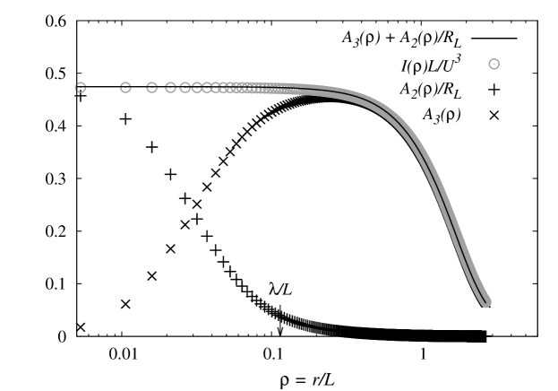
Figure 3: Dimensionless energy balance in the KHE, as expressed by Eq. (27). $R_{\lambda}=276$. The Taylor microscale is labeled for comparison. Note that the energy input is constant for scales $r<\lambda$.

Figure 3 shows the balance of energy represented by the dimensionless equation given as (27). For small scales ($\rho<\lambda/L$ for the case $R_{\lambda}=276$ shown) the input term satisfies $I(r)\simeq\varepsilon_{W}=\varepsilon$, as expected since such scales are not directly influenced by the forcing. We note that the second- and third-order structure functions may be obtained from the energy and transfer spectra, respectively, using

$$S_{2}(r)=4\int_{0}^{\infty}dk\ E(k)\left(\frac{1}{3}-\frac{\sin{kr}-kr\cos{kr}}{(kr)^{3}}\right)$$ (47)

and

$$S_{3}(r)=12r\int_{0}^{\infty}dk\ T(k)\left(\frac{3\sin{kr}-3kr\cos{kr}-(kr)^{2}\sin{kr}}{(kr)^{5}}\right)\ .$$ (48)

This procedure was introduced by Qian Qian (1997, 1999) and more recently used by Tchoufag et al Tchoufag et al. (2012) and by McComb et al McComb et al. (2014): The underlying transforms may be found in the book by Monin and Yaglom Monin and Yaglom (1975); see their Eqs. (12.75) and (12.141^′′′). From these expressions, the nonlinear and viscous terms $A_{3}$ and $A_{2}/R_{L}$ given by Eqs. (25) and (26), are calculated using

$$A_{3}(\rho)=-\frac{3L}{U^{3}}\int_{0}^{\infty}dk\ T(k)\left[\frac{\sin{kL\rho}-kL\rho\cos{kL\rho}}{(kL\rho)^{3}}\right]\ ,$$ (49)

an

$$\frac{A_{2}(\rho)}{R_{L}}=\frac{6\nu_{0}L}{U^{3}}\int_{0}^{\infty}dk\ k^{2}E(k)\left[\frac{\sin{kL\rho}-kL\rho\cos{kL\rho}}{(kL\rho)^{3}}\right].$$ (50)

Figure 4: Graph of the present DNS results for $C_{\varepsilon}$ against Reynolds number, once the estimate of the asymptote is subtracted. The effect of varying our estimate of the asymptote $C_{\varepsilon,\infty}$ is shown by the three different symbols, where $C_{\varepsilon,\infty}^{\prime}$ and $C_{\varepsilon,\infty}^{\prime\prime}$ denote variations in the asymptote within one standard error. The dashed lines represent fits of the expression $CR_{L}^{n}$ to the data after subtracting the respective values of the asymptote.

Figure 5: The same data as in Fig. 4 plotted on logarithmic scales. The solid line represents a slope of $n=-1.000\pm 0.009$, obtained from a one-parameter fit of the expression $CR_{L}^{n}$ to the data points, after subtracting the asymptote $C_{\varepsilon,\infty}=0.468$.

Figures 4 and 5 show the measured power-law dependence of $C_{\varepsilon}$ on $R_{L}$ on linear and logarithmic scales, respectively. Noting that the standard procedure of using a log-log plot to identify power-law behavior is unavailable in this case, due to the constant asymptote, we subtracted the estimated asymptotic value, which was obtained from a fit of (42) to DNS data (presented in the next section), and plotted $C_{\varepsilon}-C_{\varepsilon,\infty}$ against $R_{L}$ on linear and logarithmic scales. This allowed us to identify power-law behavior consistent with $R_{L}^{-1}$. We also tested the effect of varying our estimate of the value of the asymptote $C_{\varepsilon,\infty}$. It can be seen that the results were insensitive to this at the lower Reynolds numbers, where the $R_{L}^{-1}$-dependence is being tested. At higher $R_{L}$, the viscous contribution represented by $C/R_{L}$ becomes negligible and instead the result becomes dependent on the actual value of $C_{\varepsilon,\infty}$.

As can be seen in Fig. 4, the value of the exponent $n$ depends weakly on the variation of the asymptote. The different values of $n$ shown in the figure were obtained by performing two-parameter fits of the expression $CR_{L}^{n}$ to the data points after subtracting the respective values of the asymptote. The fits using the asymptotes $C_{\varepsilon,\infty}$, $C_{\varepsilon,\infty}^{\prime}$, and $C_{\varepsilon,\infty}^{\prime\prime}$, result in exponents consistent with a $1/R_{L}$ dependence of $C_{\varepsilon}$ on $R_{L}$, namely, $n=-1.0\pm 0.1$. The quality of the fit can be improved by fixing the coefficient $C$ to take the value $C=18.9$ obtained from the fit of (42) to data, which is presented in the following section.

IV.2 Assessment of the model

In order to test our model for the dimensionless dissipation rate, we fitted an expression of the form (42) to data obtained with the present DNS, and it was found to agree very well, as shown in Fig. 6. Measuring the exponent separately as explained in the previous section and shown in Fig 4, resulted in $n=-1.0\pm 0.1$ and so supports the model equation, with the constants given by $C_{\varepsilon,\infty}=0.468\pm 0.006$ and $C=18.9\pm 1.3$. Fixing the value of the coefficient $C$ to be $C=18.9$, as obtained by the fit of (42) to data, and by performing a one-parameter fit, varying only the exponent, results in $n=-1.000\pm 0.009$, as shown in Fig. 5.

As shown in Fig. 6 (and in Fig. 1), it may be seen that our model (42) is in good agreement with both our own data and that of others, where we note that the expression fitted to our data in Fig. 1 is equivalent to our model (42).

Figure 6: The expression given in Eq. (42) fitted to present DNS data resulting in $C_{\varepsilon,\infty}=0.468$ and $C=18.9$.

V Discussion

Our model, as given by either Eq. (42) (for dependence on $R_{L}$) or Eq. (44) (for dependence on $R_{\lambda}$), may be compared to other work in the literature. As mentioned in the Introduction, Sreenivasan Sreenivasan (1984) compared experimental results for free decay to the expression for very low Reynolds numbers,

$$C_{\varepsilon}=\frac{15}{R_{\lambda}}\sqrt{\frac{\pi}{2}}\ .$$ (51)

This used the isotropic relation $\varepsilon=15\nu_{0}U^{2}/\lambda^{2}$ (where $\lambda$ is the Taylor microscale) and the approximation $L/\lambda\simeq(\pi/2)^{1/2}\$ Batchelor (1971). Note that, while $15\sqrt{\pi/2}=18.8$, compared to $C=18.9\pm 1.3$ found in the present analysis, this expression involves $R_{\lambda}$ rather than $R_{L}$. At low $R_{L}$, however, $R_{L}\sim R_{\lambda}$; thus, by combination of the two asymptotic results in Sreenivasan’s paper Sreenivasan (1984), one obtains the result for the scaling of the dimensionless dissipation rate reported here. Furthermore, the values of the coefficient $C$ obtained by Sreenivasan and measured numerically by us agree within one standard error.

Later, Lohse Lohse (1994) used “variable range mean-field theory” to find an expression for the dimensionless dissipation coefficient by matching small $r$ and inertial range forms for the second-order structure function, and obtained

$$C_{\varepsilon} =C_{\varepsilon,\infty}\sqrt{1+\frac{5b^{3}}{4R_{\lambda}^{2}}}\ ,$$ (52)

where $b=S_{2}(r)/(\varepsilon r)^{2/3}$ such that $C_{\varepsilon,\infty}=(h_{2}(1)/b)^{3/2}$. At low Reynolds numbers, this author reported $C_{\varepsilon}=18/R_{L}$. The asymptotic value was calculated by Pearson, Krogstad and van der Water Pearson et al. (2002), who used $h_{2}(1)\simeq 1.25$ and $b\simeq 2.05$, to be $C_{\varepsilon,\infty}\simeq 0.48$, which agrees with our result, $C_{\varepsilon,\infty}=0.468\pm 0.006$, nearly within one standard error.

In an alternative approach, Doering and Foias Doering and Foias (2002) used the longest lengthscale affected by forcing, $l$, to derive upper and lower bounds on $C_{\varepsilon}$,

$$\frac{4\pi^{2}}{\alpha^{2}Re}\leq C_{\varepsilon}\leq\left(\frac{a}{Re}+b\right)$$ (53)

for constants $a,b$, where $Re=Ul/\nu_{0}$ and $\alpha=L_{\text{box}}/l$. While the upper bound resembles the present model, it is important to note that where these authors have obtained an inequality, we have an equality. Inspired by the results of Doering and Foias (2002), Eq. (44), which is equivalent to the model equation (42) and thus to the expression in the upper bound (53), was fitted to data by Donzis, Sreenivasan and Yeung Donzis et al. (2005), with $A\simeq 0.2$ and $B\simeq 92$ giving reasonable agreement, such that $C_{\varepsilon,\infty}\simeq 0.4$.

Later still, Bos, Shao and Bertoglio Bos et al. (2007) employed the idea of a finite cascade time to relate the expressions for $C_{\varepsilon}$ in forced and decaying turbulence. Using a model spectrum, they then derived a form for $C_{\varepsilon}$ and found the asymptotic value $C_{\varepsilon,\infty}=0.53$ with the Kolmogorov constant $C_{K}=1.5$. Note that when we used their formula, with the value $C_{K}=1.625$ instead (which is probably more representative McComb (2014)), this led to $C_{\varepsilon,\infty}=0.47$, as found in the present work. With a simplified model spectrum, the authors then showed how their expression reduced to $C_{\varepsilon}=19/R_{L}$ for low Reynolds numbers [when $E(k)\sim k^{4}$ at low $k$] in agreement with $C=18.9\pm 1.3$ found here (within one standard error).

We finish with a brief consideration of the universality of these results. In general this would mean that the $C_{\varepsilon}$ versus $R_{\lambda}$ curve would take the same form for all flow configurations, such as pipe flow, free jets, isotropic turbulence, and so on. Evidently, as our present work is restricted to stationary isotropic turbulence, this rather restricts what we can say about the matter. Indeed, we basically can only consider the effects of the initial conditions such as the form of the forcing and the shape of the initial spectrum, and insofar as these have been tested, our brief literature survey would indicate that they probably only affect the duration of transient behavior, but not the steady-state results. This is, of course, in line with what one expects from universality of isotropic turbulence in general. That is, forcing should be confined to low wavenumbers in order to set up an asymptotic state which is representative of the equations of motion, rather than the arbitrarily chosen forcing. Similarly, the arbitrary initial energy spectrum should quickly die away to be replaced by the true spectrum. So it is important to recognize that the universality of the $C_{\varepsilon}$ curve should be considered in conjunction with the universality of the turbulence that we are producing. Our present work suggests that the model based on $\delta$-function forcing is in good agreement with the DNSs based on finite (in wavenumber space) forcing, and that the values of the constants $C$ and $C_{\varepsilon,\infty}$ agree quite well with those obtained in other investigations. This might be seen as evidence for universality within the confines of this particular flow. Certainly one should observe that the scatter of points from various investigations in Fig. 1 is not evidence of nonuniversality, unless one has eliminated other possible explanations for this scatter, such as differences in run time or resolution.

We made a systematic investigation into the effect of run time on the measured value of $C_{\varepsilon}$ for our highest $R_{L}$ data point. In total, this run was carried out for about 12 large-eddy turnover times in steady state, resulting in the measured value of $C_{\varepsilon}=0.466\pm 0.021$. If we restrict the time interval that we average results over to, say, 3 large-eddy turnover times, we measure $C_{\varepsilon}=0.442\pm 0.030$, which is significantly lower than the measured value averaged over the full run. Note that the value obtained from the shorter time interval is closer to some of the values measured by other groups shown in Fig. 1.

Then, by extending the time interval systematically towards the actual run time in steady state, we found that the results converged to the value obtained by averaging over the full time interval. Work on this aspect continues as part of our program on DNS and will be reported in due course.

VI Conclusions

Our theoretical model predicts an inverse dependence of the dimensionless dissipation rate on the integral scale Reynolds number, with asymptotic validity in the limit of large Reynolds numbers. A question then arises: Do we have to include higher-order terms at lower Reynolds numbers? It is in order to answer this question that we resort to direct numerical simulation.

The answer to our question is reassuring. We find that analysis of the data from our DNS supports a dependence on $R_{L}^{-1}$ at all values of the Reynolds number. Also, the law given by Eq. (42) is found to give a good fit to the data from the DNS, with values for the constants which are in generally good agreement with those obtained in other investigations.

It may be of interest to note, that when we apply the same theoretical approach to magnetohydrodynamics (MHD), we find that it is necessary to take the term in $R_{L}^{-2}$ into account, in addition to the leading order term, although the effect was not large Linkmann et al. (2015). We also plan to extend the analysis to inhomogeneous flows, in order to examine further the question of universality, as discussed at the end of the preceding section.

Last, we note that our analysis shows that the behavior of the dimensionless dissipation rate, as found experimentally, is entirely in accord with the Kolmogorov (K41) picture of turbulence and, in particular, with Kolmogorov’s derivation of his four-fifths law Kolmogorov (1941), the one universally accepted result in turbulence.