Flow Allocation for Maximum Throughput and Bounded Delay on Multiple Disjoint Paths for Random Access Wireless Multihop Networks

Abstract

In this paper, we consider random access, wireless, multi-hop networks, with multi-packet reception capabilities, where multiple flows are forwarded to the gateways through node disjoint paths. We explore the issue of allocating flow on multiple paths, exhibiting both intra- and inter-path interference, in order to maximize average aggregate flow throughput (AAT) and also provide bounded packet delay. A distributed flow allocation scheme is proposed where allocation of flow on paths is formulated as an optimization problem. Through an illustrative topology it is shown that the corresponding problem is non-convex. Furthermore, a simple, but accurate model is employed for the average aggregate throughput achieved by all flows, that captures both intra- and inter-path interference through the SINR model. The proposed scheme is evaluated through Ns2 simulations of several random wireless scenarios. Simulation results reveal that, the model employed, accurately captures the AAT observed in the simulated scenarios, even when the assumption of saturated queues is removed. Simulation results also show that the proposed scheme achieves significantly higher AAT, for the vast majority of the wireless scenarios explored, than the following flow allocation schemes: one that assigns flows on paths on a round-robin fashion, one that optimally utilizes the best path only, and another one that assigns the maximum possible flow on each path. Finally, a variant of the proposed scheme is explored, where interference for each link is approximated by considering its dominant interfering nodes only.

I Introduction

In order to better utilize the scarce resources of wireless multi-hop networks and meet the increased user demand for QoS, numerous studies have suggested the use of multiple paths in parallel. Utilization of multiple paths can provide a wide range of benefits in terms of, throughput [2, 3, 4], delay [5, 3, 4], reliability [6, 3, 4], load balancing [7, 2], security [8] and energy efficiency [7, 9]. However, multipath utilization in wireless networks, is more complicated compared to their wired counterparts, since transmissions across a link interfere with neighbouring links, reducing thus, network performance.

I-A Related work

A wide range of different schemes, have been proposed in literature, focusing on multipath utilization for improving network performance, including routing schemes, resource allocation, flow control, opportunistic-based forwarding ones, e.t.c. A significant amount of studies focuses on identifying the set of paths that will guarantee improved performance, in terms of some metric [2, 5, 10, 11]. However, such studies, mostly address the issue of, which paths should be utilized and rely on heuristic-based approaches concerning the issue of how, should these paths be utilized. In [10] for example, traffic is allocated on a round-robin fashion among the available paths.

Several studies suggest schemes that perform joint scheduling with routing, power control or channel assignment [12, 13, 14]. As far as, flow allocation on multiple paths and rate control are concerned, a well studied approach associates a utility function to each flow’s rate and aims at maximizing the sum of these utilities, subject to cross-layer constraints. Along this direction, several studies suggest, joint congestion control and scheduling approaches [15, 16, 17]. Authors in [18], instead of employing a utility function of a flow’s rate, they employ a utility function of flow’s effective rate, in order to take into account the effect of lossy links. Different from these approaches, this work considers random access networks and also no scheduling is assumed, or devised.

The utility maximization framework, has also been applied in the context of random access networks for designing joint congestion and contention control schemes [19, 20]. As far as the interference model in these studies is concerned, no capture is assumed and thus, concurrent transmissions on interfering links fail each other. A joint routing and MAC control scheme, for wireless random access networks, is explored in [21], where interference is modelled through conflict sets and the SINR model. Different from all these studies, this work considers wireless random access networks, where interference is captured through the SINR model, taking also into account the effect of Rayleigh fading on signal attenuation.

Authors in [22], study an MPLS-based forwarding paradigm and aim at identifying a feasible routing solution, for multiple flows deploying multiple paths. Links whose transmissions have a significant effect on each others success probability, are considered to belong to the same collision domain and cannot be active at the same time. In [23], a technique for combining multipath forwarding with packet aggregation, over IEEE802.11 wireless mesh networks, is suggested. Multipath utilization is accomplished by employing Layer-2.5, a multipath routing and forwarding strategy, that aims at utilizing links in proportion to their available bandwidth. Authors in [24], suggest a distributed rate allocation algorithm, aimed at minimizing the total distortion of video streams, transmitted over wireless adhoc networks. In [25], a max-min fair scheduling allocation algorithm is proposed, along with a modified backoff algorithm, for achieving long term fairness. In [26], a distributed flow control algorithm, aimed at maximizing the total traffic flowing from sources to destinations, also providing network lifetime guarantees, is proposed. Based on the theoretical ideas of back-pressure scheduling and utility maximization, Horizon [27], constitutes a practical implementation of a multipath forwarding scheme that interacts with TCP.

There is also a significant amount of studies that suggest opportunistic forwarding/routing schemes that exploit the broadcast nature of the wireless medium. [28], suggests a multipath routing protocol called Multipath Code Casting that employs opportunistic forwarding combined with network coding. It also performs congestion control and employs a rate control mechanism, that achieves fairness among different flows, by maximizing an aggregate utility of these flows. Authors in [29], suggest an optimization framework that performs optimal flow control, routing, scheduling and rate adaptation, employing multiple paths and opportunistic transmissions. Other works consider network-level cooperation combining queueing analysis but focusing on simple topologies [30, 31, 32].

I-B Contributions

Different from all the above, in this study, we consider wireless, random access, multihop networks, with multi-packet reception capabilities, where multiple unicast flows are forwarded to their destinations through multiple paths that share no common nodes (node disjoint paths). It should also be noted that, the assumption of random access implies that transmitters get access to the shared medium in a decentralized manner, without presupposing any coordination method. We address the problem of allocating flow data rates on paths in such a way that they maximize the average aggregate flow throughput, while also providing bounded packet delay, in the presence of both intra- and inter-path interference, for the aforementioned type of networks. For the rest of the paper, we will refer to this problem as the flow allocation problem. The main contribution of this study, is a scheme that formulates flow rate allocation as an optimization problem. The key feature of this scheme is its distributed nature; the information that is needed to be propagated for each node through the routing protocol is the position of each node, an indication of whether a node is a flow source, relay, or sink and the transmission probability in case of a relay node. With this information available, each node can infer its own instance of the topology and also its own instance of the aforementioned flow allocation problem. Each flow source can then solve this problem, independently of all other sources in order to derive flow rates that collectively, maximize AAT. Another key feature of the proposed scheme, is that it maximizes the average aggregate throughput (AAT) achieved by all flows, while also providing bounded packet delay guarantees. For the rest of this study we will refer to this scheme as, the Throughput Optimal Flow Rate Allocation scheme, or TOFRA, for reasons of brevity. The proposed scheme is based on a simple, but accurate model for the average aggregate throughput, capturing both inter- and intra-path interference through the SINR model. Additionally, the effect of Rayleigh fading is also taken into account for deriving a link’s success probability. Through a simple topology we show that the corresponding flow allocation optimization problem is non-convex. Another contribution of the study, is the evaluation of the proposed scheme, through Ns2 simulations of several random wireless scenarios.

In the evaluation process, the accuracy of the model, for capturing the AAT observed in the simulation scenarios, is explored. Simulation results show that, the model employed by the proposed scheme, accurately captures the AAT observed in the simulation results, even when the assumption of saturated queues is removed. In the second part of the evaluation process, we compare the AAT achieved by the proposed flow allocation scheme with the following flow allocation schemes: Best-path, that optimally utilizes the best path available, Full MultiPath, that assigns the maximum possible flow (one packet per slot) on each path, and a Round-Robin based one. For all simulated scenarios and all SINR threshold values considered, the proposed scheme achieves significantly higher throughput than full multipath and Best-path. Additionally, the proposed scheme outperforms round robin-based flow allocation for the vast majority of the scenarios explored. Finally, a key contribution of the study is that we also explore a variant of the proposed scheme, where interference for a link is approximated by considering the dominant interfering nodes for that link only. More precisely, we explore the trade-off between accurately capturing the AAT observed in the simulation scenarios and the complexity in formulating and solving, the corresponding optimization problem.

The rest of the paper is organized as follows: Section II, presents the system model considered. In Section III, we present the proposed flow allocation scheme and demonstrate it through a simple topology. In Section IV, we describe the simulation setup and present the evaluation process. We conclude this study in Section V.

II System Model

We consider static, wireless, multi-hop networks, with the following properties:

• Random access to the shared medium where each node transmits independently of all other nodes, based on its transmission probability. In this way, no coordination among nodes is required thus, random access is a fully distributed access protocol. For flow originators, transmission probability denotes the rate at which they inject packets into the network (flow rate). For the relay nodes, transmission probability is fixed to a specific value and no control is assumed.

• Time is slotted and each packet transmission requires one timeslot.

• Flows among different pairs of source and destination nodes, carry unicast traffic of same-sized packets.

• All nodes use the same channel and rate, and are equipped with multi-user detectors being thus, able to successfully decode packets from more than one transmitter at the same slot [33].

• We assume that all nodes are half-duplex and thus, cannot transmit and receive simultaneously.

• We also assume that, all nodes always have packets available for transmission. However, in the evaluation process, we also consider the case that the nodes can have empty queues. As illustrated in Section IV-B, there is no significant impact on the AAT.

• As far as routing is concerned, multiple, node disjoint paths are assumed to be available by the routing protocol, one for each flow. Moreover, source routing is assumed, ensuring that packets of the same flow are routed to the destination along the same path. Apart from that, for each node, its position, transmission probability, or flow rate, along with an indication of whether it is a flow originator, relay, or sink, are assumed known to all other nodes. This information can be periodically propagated throughout the network through a link-state routing protocol.

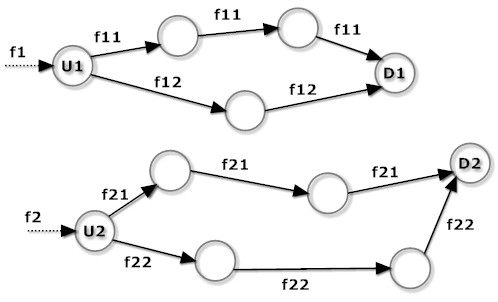
(a) Wireless multi-hop mesh network

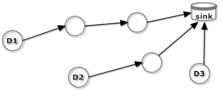
(b) Sensor network

Figure 1: Wireless scenarios where throughput optimal flow allocation is applicable.

Fig. 1(a) and Fig. 1(b), present two different wireless settings, where the suggested flow allocation scheme may be employed. In the first scenario, depicted in Fig. 1(a), different users (U1 and U2), generate flows (f1, f2), that are routed to destination nodes D1 and D2, respectively, through node disjoint multi-hop paths. These flows can be split into multiple subflows, in order to aggregate network resources and achieve higher aggregate throughput. The suggested flow allocation framework can be applied, in order to identify the data rates for subflows f11, f12, f21, and f22 that result in maximum average aggregate throughput for both users.

The second scenario, depicted in Fig. 1(b), represents a sensor network, where multiple sensor nodes generate data (D1, D2, and D3), that are forwarded to the sink, through multiple paths comprised by relay sensor nodes. The proposed flow allocation scheme can be employed for maximizing the rate at which the sink receives data from the sensor nodes.

II-A Physical Layer Model

Notation	Definition
$T$	Set of concurently active transmitters with
	link $(i,j)$
$\alpha$	Path loss exponent
$\eta_{j}$	Receiver noise power at $j$
$\gamma_{j}$	SINR threshold at $j$
$P_{tx}(i)$	Transmitting power of node $i$
$A(i,j)$	Random variable for channel fading over
	link $(i,j)$
$v(i,j)$	Prameter of the Rayleigh random variable for
	fading over link $(i,j)$
$r(i,j)$	Distance between nodes $i$, and $j$
$g(i,j)$	Received power factor for link $(i,j)$
$P_{rx}(i,j)$	Received power over link $(i,j)$
$p_{i/T}^{j}$	Success probability for link $(i,j)$, given that
	nodes in $T$ are concurrently active
$q_{i}$	Transmission probability for node $i$, given there
	is packet for transmission in its queue

TABLE I: System model related notations

The MPR channel model used in this paper is a generalized form of the packet erasure model. Note that, the notations used for presenting the channel model considered, are also summarized in Table I. In the wireless environment, a packet can be decoded correctly by the receiver, if the received $SINR$ exceeds a certain threshold. More precisely, suppose that a set of nodes, denoted by $T$, is concurrently active with transmitting node $i$, in the same time slot. Let $P_{rx}(i,j)$ be the signal power received from node $i$ at node $j$. Let $SINR(i,j)$ be expressed using (1).

$$SINR(i,j)=\frac{P_{rx}(i,j)}{\eta_{j}+\sum_{k\in T\backslash\left\{i\right\}}{P_{rx}(k,j)}}.$$ (1)

In the above equation, $\eta_{j}$ denotes the receiver noise power at $j$. We assume that a packet transmitted by $i$, is successfully received by $j$, if and only if, $SINR(i,j)\geq\gamma_{j}$, where $\gamma_{j}$ is a threshold characteristic of node $j$. The wireless channel is subject to fading; let $P_{tx}(i)$ be the transmitting power of node $i$ and $r(i,j)$ be the distance between $i$ and $j$. The power received by $j$, when $i$ transmits, is $P_{rx}(i,j)=A(i,j)g(i,j)$, where $A(i,j)$ is a random variable representing channel fading. Under Rayleigh fading, it is known [34] that $A(i,j)$ is exponentially distributed. The received power factor, $g(i,j)$, is given by $g(i,j)=P_{tx}(i)(r(i,j))^{-\alpha}$, where $\alpha$ is the path loss exponent, with typical values between $2$ and $4$. The success probability of link $(i,j)$, when the transmitting nodes are in $T$, is given by:

$$p_{i/T}^{j}=\exp\left(-\frac{\gamma_{j}\eta_{j}}{v(i,j)g(i,j)}\right)\prod_{k\in T\backslash\left\{i,j\right\}}{\left(1+\gamma_{j}\frac{v(k,j)g(k,j)}{v(i,j)g(i,j)}\right)}^{-1},$$ (2)

where $v(i,j)$ is the parameter of the Rayleigh random variable for fading. The analytical derivation for this success probability, which captures the effect of interference on link $(i,j)$, from transmissions of nodes in set $T$, can be found in [35].

III Throughput optimal flow rate allocation (TOFRA) scheme

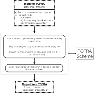
Figure 2: Diagram of the proposed distributed flow allocation (TOFRA) scheme.

In this section, the main concepts of the proposed flow allocation scheme are presented. First, the input required by the proposed flow allocation scheme, from the routing protocol, is presented. This input is used for calculating flow rates that maximize average aggregate flow throughput (AAT), on a distributed manner at each source. In Section III-A, the analysis employed for formulating flow rate allocation as an optimization problem is presented. The proposed scheme is demonstrated through a simple topology in Section III-B.

Introducing some of the notations, also required for the analysis presented in Section III-A, we assume $m$ flows, $f_{1},f_{2},...,f_{m},$ that need to forward traffic to their destinations. For flow $f_{i}$, let $Src(f_{i})$ denote its source. As also shown in Fig. 2, it is assumed that the routing protocol, provides each flow source, $Src(f_{i})$, with a path to its corresponding destination, namely, $r_{i}$. It is further assumed that, these paths are node-disjoint thus, they do not share common nodes. Implementing though, a routing protocol that identifies the path to be utilized, for each source and destination pair, is out of the scope this study. However, it should be noted that, the proposed flow allocation scheme is independent of the routing protocol implementation.

As already stated in the Introduction, the goal of the proposed scheme is to maximize AAT, while also providing bounded delay. Along this direction, the flow rate with which, each source injects traffic, on the path employed, needs to be calculated. An additional requirement for the proposed scheme is that, flow rate estimation should be distributed. For that reason, each flow source, should estimate independently of all other sources, the rate of the flow injected, that contributes to achieving the maximum AAT for all flows. For doing so, each flow needs to infer its own view of the network topology and derive its own instance of the flow allocation optimization problem, presented in the next section. As Fig. 2 shows, for deriving its own instance of the flow allocation problem, each flow source is required to know for each other network node the following information: a) node position, b) type of node (source, relay, or sink), and c) transmission probability for relays. Node positions for example, can be used to derive link distances, and thus success probability for each link, based on (2) of Section II. As also presented in Fig. 2, this information can be available for each node, throughout the network, through the routing protocol. After having inferred its own instance of the flow allocation optimization problem, it can solve it and derive the flow rates that flow sources should assign on each path, in order to collectively maximize AAT.

III-A Analysis

In this section, we present how aggregate throughput optimal flow rate allocation is formulated, at each flow source, as an optimization problem, for random topologies. The suggested scheme is also demonstrated through a simple topology in order to provide insights that are difficult to obtain through larger topologies.

Notation	Definition
$V$	Set of nodes. $|V|=N$
$f_{1},f_{2},...,f_{m}$	$m$ flows
$r_{i}$	Path $i$ employed by flow $f_{i}$
$R=\{r_{1},r_{2},...,r_{m}\}$	Set of node disjoint paths
$|r_{i}|$	Num of links in path $r_{i}$
$I_{i,j}$	Interfering nodes for link ($i$,$j$)
$I_{i,j}[n]$	Id of nth interfering node for
	link (i,j)
$L_{i,j}=|I_{i,j}|$	Number of nodes that interfere
	with transmissions on (i,j)
$Src(r_{k})$	Source node of the $k^{th}$ flow
$P_{r_{k}}=\prod_{(i,j)\in r_{k}}p_{i/i}^{j}$	End-to-end success probability
	for path $r_{k}$
$\bar{T}_{i,j}$	Average throughput for (i,j)
	(Pkts/slot)
$\bar{T}_{r_{k}}$	Average throughput for $k^{th}$
	flow (Pkts/slot)

TABLE II: Flow allocation problem related notations

The suggested method for formulating aggregate throughput optimal flow rate allocation as an optimization problem for random topologies is a procedure consisting of two steps (also depicted in Fig. 2). We demonstrate this procedure assuming multiple flows that are forwarded to the same destination. The same analysis however can be applied for the case where multiple flows have different destination nodes. First, the notations used in the analysis, are presented and are also summarized in Table II. V denotes the set of the nodes and $|V|=N$. As also stated in the previous section, we assume $m$ flows $f_{1},f_{2},...,f_{m},$ that need to forward traffic to the destination node $D$. $R=\{r_{1},r_{2},...,r_{m}\}$ represents the set of $m$ disjoint paths employed by these flows. $|r_{i}|$ is used to denote the number of links in path $r_{i}$. $I_{i,j}$ is the set of nodes that cause interference to packets sent from i to j. For example, if all network nodes are assumed to contribute with interference to link $(i,j)$ and $j\neq D$, then $I_{i,j}=V\setminus\{i,j,D\}$ and thus, the set of nodes that cause interference to that link has size $L_{i,j}=|I_{i,j}|=|V|-3$. Further on, $Src(r_{k})$ is used to denote the source node of the $k^{th}$ flow, employing path $r_{k}$. $\bar{T}_{i,j}$ and $\bar{T}_{r_{k}}$, denote the average throughput, measured in packets per slot, achieved by link $(i,j)$ and flow $f_{k}$ forwarded over path $r_{k}$, respectively. Finally, $I_{i,j}[n]$ denotes the id of the n^th interfering node for link $(i,j)$.

The first step of the suggested method, presented as Step $1$ in Fig. 2, consists of deriving the expression for the average throughput of a random link $(i,j)$.

$$\bar{T}_{i,j}=\sum_{l=0}^{2^{L_{i,j}}-1}P_{i,j,l}q_{i,j}\prod_{n=1}^{L_{i,j}}q_{I_{i,j}[n]}^{b(l,n)}(1-q_{I_{i,j}[n]})^{1-b(l,n)},$$ (3)

where

$$q_{i,j}=\left\{\begin{matrix}&q_{i}\quad&j=D\\ &q_{i}(1-q_{j})\quad&j\neq D\\ \end{matrix}\right.,$$

$$P_{i,j,l}=p_{i/i\cup\{I_{i,j}[n],\;\forall\;n:\;b(l,n)\neq 0)\}}^{j},$$

$$b(l,n)=l\;\&\;2^{n-1},\;\text{\& is the logical bitwise AND operator.}$$

Average throughput for that link, $\bar{T}_{i,j}$, can be expressed as the probability of having a successful packet reception over link $(i,j)$ and is given through (3).

The probability of a successfull packet transmission along link $(i,j)$ during a slot, depends among others, on the amount of received interference. However, the amount of received interference also depends on the set of neighboring nodes that are transmitting in each slot. Thus, the expression for a link’s $(i,j)$ average throughput, requires the enumeration of all possible subsets of interfering nodes. More precisely, assuming that $L(i,j)$ denotes the set of all nodes that cause interference to the transmissions over the link $(i,j)$, all possible different subsets of active interfering nodes are $2^{L(i,j)}$. In each timeslot thus, there are $2^{L(i,j)}$ different cases where a packet transmission may be successful for link $(i,j)$. The probability of a successful packet transmission for link $(i,j)$, for all $2^{L(i,j)}$ cases, is captured through the summation term in equation (3). In this equation, index $l$ runs from $0$ to $2^{L(i,j)}-1$, enumerating all possible different subsets of active interfering nodes. Let $I_{l}^{i,j}$ for example, denote the $l^{th}$ subset of interfering nodes for link $(i,j)$. The probability of a successful packet transmission over that link when all nodes in $I_{l}^{i,j}$ are actvive at the same timeslot, is derived by considering the transmission probability of the nodes participating in $I_{l}^{i,j}$ and the success probability of link $(i,j)$ given the interference by every transmitter in $I_{l}^{i,j}$. Note that, as also shown in Table I, a node i, is active during a slot with probability $q_{i}$. For flow originators, $q_{i}$ denotes flow rate. As also described in Section II, transmission probability and position for every node, can be periodically propagated to all other nodes, through routing protocol’s control messages. The success probability of link $(i,j)$, given the interference from nodes in $I_{l}^{i,j}$, is captured through term $P_{i,j,l}$ in equation (3). $P_{i,j,l}$ is in essence calculated through $p_{i/T}^{j}$ in equation 2 where $T$ in this case is the $I_{l}^{i,j}$. Finally, it should be noted that, $b(l,n)$ in equation (3) becomes one if the $n^{th}$ node in $I_{i,j}$ is assumed active in the $l^{th}$ subset examined.

For large networks though, enumerating all subsets of active transmitters may be computationally intractable. In Section IV though, we explore a variant of the suggested flow allocation scheme, where only the k dominant interfering nodes are taken into account for expressing the throughput of link $(i,j)$. As also discussed in that section, dominant interfering nodes for that link, are considered those that impose the most significant amount of interference to packets received by j.

The average aggregate throughput, achieved by all flows, is expressed through $\bar{T}_{aggr}=\sum_{k=1}^{m}\bar{T}_{r_{k}}$, where $\bar{T}_{r_{k}}=\underset{(i,j)\in r_{k}}{min}\bar{T}_{i,j}$. The second step of the suggested method, also depicted in Fig. 2, consists of maximizing the average aggregate throughput, while also guaranteeing bounded packet delay which results in non-smooth optimization problem P1:

$$\underset{S}{\text{Maximize}}\sum_{k=1}^{m}\underset{(i,j)\in r_{k}}{min}\bar{T}_{i,j}\quad\quad\quad\quad\quad\quad(P1)$$

s.t:

$$(S1):\;0\leq q_{Src(r_{k})}\leq 1,\;k=1,...,m$$

$$(S2):\;\bar{T}_{Src(r_{k}),i}\leq\bar{T}_{j,l},$$

$$\quad\quad\quad\{\forall i,j,k,l:(Src(r_{k}),i),\;(j,l)\in r_{k},|r_{k}|>1$$

$$\quad\quad\quad k=1,...,m\},$$

where $S=\{q_{Src(r_{k})},\;k=1,...,m\}$. Constraint set S1 ensures that, the maximum data rate for any flow, does not exceed one packet per slot, while also allowing paths to remain unutilized. Constraint S2 ensures that, the flow injected on each path, that is the throughput of that path’s first link, is limited by the flow that can be serviced by any subsequent link of that path. In this way, data packets are prevented from accumulating at the relay nodes, guaranteeing thus, bounded packet delay. For the rest of the paper, this constraint will be referred to as bounded delay constraint.

P1 can be transformed to the following smooth optimization problem:

$$\underset{S^{\prime}}{\text{Maximize}}\sum_{k=1}^{m}\left\{\begin{matrix}\bar{T}_{Src(r_{k}),D},&|r_{k}|=1\quad\quad\quad\quad\quad(P2)\\ q^{\prime}_{Src(r_{k})},&|r_{k}|>1\quad\quad\quad\quad\quad\quad\quad\quad\end{matrix}\right.$$

$$s.t.:$$

$$\quad\quad(S1):\;0\leq q_{Src(r_{k})}\leq 1,\;k=1,...,m$$

$$\quad\quad(S2):\;\bar{T}_{Src(r_{k}),i}\leq\bar{T}_{j,l},$$

$$\quad\quad\quad\quad\quad\{\forall i,j,k,l:(Src(r_{k}),i),\;(j,l)\in r_{k},|r_{k}|>1$$

$$\quad\quad\quad\quad\quad k=1,...,m\}$$

$$\quad\quad(S3):\;0\leq q^{\prime}_{Src(r_{k})}\leq 1,\;\{\forall k:|r_{k}|>1\}$$

$$\quad\quad(S4):\;q^{\prime}_{Src(r_{k})}\leq\bar{T}_{i,j},\;\{\forall i,j,k:|r_{k}|>1,\;(i,j)\in r_{k}\},$$

where $S^{\prime}=\{q_{Src(r_{k})},\;k=1,...,m\}\cup\{q^{\prime}_{src(r_{k})}:\;|r_{k}|>1\}$. For the rest of the paper, we will refer to optimization problem P2 above as, the flow allocation optimization problem.

III-B Throughput optimal flow rate allocation: An illustrative scenario

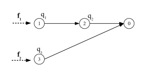
Figure 3: An illustrative topology.

We consider the simple topology presented in Fig. 3. This simple topology is used to illustrate key features of the proposed scheme and also to provide insights concerning the relation among the flow allocation on each path, interference, and SINR threshold employed. Such insights are hard to obtain from more complex scenarios. Two flows namely, $f_{1}$ and $f_{2}$, originating from nodes $1$, and $3$, are forwarded to destination node $0$ through paths $r_{1}$: $1\rightarrow 2\rightarrow 0$ and $r_{2}$: $3\rightarrow 0$, respectively. We further assume that, transmissions on a specific link, cause interference to all other links. Before presenting each link’s average throughput, consider link $(2,0)$ as an example. Transmitters that cause interference to packets sent from $2$ to $0$, constitute set $I_{2,0}=\{1,3\}$ and thus $L_{2,0}=2$. There are three possible subsets of nodes that may cause interference on link $(2,0)$ : $\{1\},\{3\},\{1,3\}$. When $l=3$, in (3), it indicates the third subset of interfering nodes, with $b(l,n)$ becoming one, for both $n=1$ and $n=2$.

The average throughput per link is presented in (4a)-(4c).

$${\bar{T}}_{1,2} =q_{1}(1-q_{2})(1-q_{3})p_{1/1}^{2}+q_{1}(1-q_{2})q_{3}p_{1/1,3}^{2}$$ (4a)

$${\bar{T}}_{2,0} =q_{2}(1-q_{1})(1-q_{3})p_{2/2}^{0}+q_{2}q_{1}(1-q_{3})p_{2/2,1}^{0}$$

$$+q_{2}(1-q_{1})q_{3}p_{2/2,3}^{0}+q_{2}q_{1}q_{3}p_{2/1,2,3}^{0}$$ (4b)

$${\bar{T}}_{3,0} =q_{3}(1-q_{1})(1-q_{2})p_{3/3}^{0}+q_{3}q_{1}(1-q_{2})p_{3/1,3}^{0}$$

$$+q_{3}(1-q_{1})q_{2}p_{3/2,3}^{0}+q_{3}q_{1}q_{2}p_{3/1,2,3}^{0}$$ (4c)

Recall that, $q_{1}$ and $q_{3}$, denote the data rates for flows, $f_{1}$ and $f_{2}$, respectively. Aggregate average throughput achieved by all flows can be expressed through (5).

$${\bar{T}}_{aggr}={\bar{T}}_{r_{1}}+{\bar{T}}_{r_{2}},\quad where,$$ (5)

$${\bar{T}}_{r_{1}}=min\{{\bar{T}}_{1,2},{\bar{T}}_{2,0}\},\quad{\bar{T}}_{r_{2}}={\bar{T}}_{3,0}$$

Average aggregate throughput-optimal flow rate allocation, consists of identifying rates, $q_{1}$ and $q_{3}$, that maximize average aggregate throughput, while also guaranteeing bounded packet delay. These rates can be found by solving the following optimization problem:

$$\underset{q_{1},q_{3}}{\text{Maximize}} {\bar{T}}_{30}+min\{{\bar{T}}_{12},{\bar{T}}_{20}\}$$

subject to $$0\leq q_{i}\leq 1,\;i\in\{1,3\}\quad(g1)-(g4)\quad\quad\quad$$

$${\bar{T}}_{12}\leq{\bar{T}}_{20}\quad\quad\quad\quad\quad\quad(g5)$$

Constraint (g5) constitutes the bounded delay constraint for path $r_{1}$. The above non-smooth optimization problem can be transformed to the following smooth optimization problem:

$$\underset{q_{1}^{{}^{\prime}},q_{1},q_{3}}{\text{Maximize}} {\bar{T}}_{30}+q_{1}^{{}^{\prime}}$$

subject to $$0\leq q_{i}\leq 1,\;i\in\{1,3\}\quad (g1) -(g4)$$

$${\bar{T}}_{12}\leq{\bar{T}}_{20}, (g5)$$

$$q_{1}^{{}^{\prime}}\leq{\bar{T}}_{12}, (g6) \quad\quad\quad\quad(P3)$$

$$q_{1}^{{}^{\prime}}\leq{\bar{T}}_{20}, (g7)$$

$$0\leq q_{1}^{{}^{\prime}}\leq 1 (g8) -(g9)$$

Transforming the above optimization problem in the standard form, the function over $q_{1}^{{}^{\prime}},q_{1},q_{3}$ related to constraint (g5), $g_{5}(q_{1}^{{}^{\prime}},q_{1},q_{3})={\bar{T}}_{12}-{\bar{T}}_{20}$ is non-convex and thus the problem is non-convex.

Before presenting simulation results for random wireless scenarios, we further motivate flow rate allocation on multiple paths, using numerical results derived from the simple topology depicted in Fig 3. Let $d(i,j)$ denote the distance between nodes $i$ and $j$. Let also, $P_{r_{k}}=\prod_{(i,j)\in r_{k}}p_{i/i}^{j}$, denote the end-to-end success probability, for path $r_{k}$. For the illustrative purpose of this section, we assume that $d(1,2)=d(2,0)=d(3,1)=d$, $d(3,0)=\sqrt{5}d$, $d(3,2)=\sqrt{2}d$, where $d=400m$. Further on, the path loss exponent assumed is $3$, while the transmission probability for relay node $2$, is $0.5$. Flow rates, $q_{1}$ and $q_{3}$, that achieve maximum average aggregate throughput (AAT), for SINR threshold values $\gamma=\{0.25,0.5,...,2\}$, are estimated by solving the optimization problem (P3) using the simulated annealing technique. It should be noted that, multi-hop path $r_{1}$: $1\rightarrow 2\rightarrow 0$ exhibits higher end-to-end success probability than path $r_{2}$: $3\rightarrow 0$, for all $\gamma$ values considered.

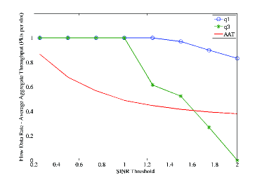
Figure 4: Optimal Flow rates and Average Aggregate Throughput achieved.

In Fig. 4, we present throughput optimal flow rates assigned on paths, $r_{1}$ and $r_{2}$, along with the average aggregate throughput achieved (AAT), for the aforementioned $\gamma$ values. As this figure shows, the maximum AAT is achieved by full rate utilization of both paths, for SINR threshold values up to $1.0$, suggesting that inter-flow interference is balanced by the gain in throughput. For SINR threshold values larger than $1.0$, utilization of path $r_{2}$, which exhibits lower performance in terms of end-to-end success probability, declines. This is due to the fact that, for large SINR threshold values, the effect of interference imposed on path $r_{1}$ becomes more significant. At the same time, the flow forwarded through path $r_{2}$, manages to deliver only a small portion of its traffic to destination node $0$.

IV Evaluation

IV-A Simulation setup

The proposed throughput optimal flow rate allocation (TOFRA) scheme, is evaluated using the network simulator Ns2, version 2.34 [36].

Parameter	Value
Max Retransmit Threshold	$3$
Transmit Power	$0.1$ Watt
Noise power	$7\times 10^{-11}$ Watt
Contention Window	5
Packet size	$1500$ Bytes
Path loss exponent	4

TABLE III: Network parameters used for deriving numerical and simulation results

Concerning medium access control, a slotted aloha-based MAC layer is implemented. Transmission of data, routing protocol control and ARP packets is performed at the beginning of each slot, without performing carrier sensing prior to transmitting. Acknowledgements for data packets are sent immediately after successful packet reception, while failed packets are retransmitted. Slot length, $T_{slot}$, is expressed through: $T_{slot}=T_{data}+T_{ack}+2D_{prop}$, where $T_{data}$ and $T_{ack}$, denote the transmission times for data packets and acknowledgements (ACKs), while $D_{prop}$ denotes the propagation delay. It should be noted that, all packets have the same size, shown in Table III. All network nodes, apart from sources of traffic, select a random number of slots before transmitting, drawn uniformly from $[0,CW]$. The contention window (CW) is fixed for the whole duration of the simulation and equal to $5$.

As far as physical layer is concerned, all data packets are successfully decoded if their received SINR exceeds the SINR threshold. The received SINR for each packet is calculated through (1). The path loss exponent is assumed to be $\alpha=4$. Transmitters during each slot, that are considered to cause interference, are those transmitting data packets, or routing protocol control packets. All nodes use the same SINR threshold, transmission rate, and channel. Transmission power and noise is $0.1$ Watt and $7\times 10^{-11}$ Watt, respectively.

As far as routing is concerned, a multipath, source-routed link-sate routing protocol based on UM-OLSR [37], is implemented. Hello and Topology Control (TC) messages are periodically propagated throughout the network. Each topology control message may carry the following information: a) transmission probability b) position, and c) an indication of whether it is a flow originator, relay or, sink. As also discussed in Section II, transmission probabilities are assumed to be fixed for relay nodes, since contention window (CW) remains fixed for the whole simulation period. For flow originators, transmission probabilities are estimated by solving the corresponding version the flow allocation optimization problem (presented in Section III-A), using the simulated annealing technique. Identification of the multiple, node-disjoint paths to be utilized by the various flows, can be performed at flow sources each time a new TC message is received. However, the main focus of the study, is not on identifying the set of paths that should be employed, but on how should these paths be utilized in order to maximize average aggregate throughput for all flows, with how referring to the amount of flow assigned on each path. We thus, employ a simple algorithm that provides traffic sources with multiple, link-disjoint, least-cost paths. The multipath set is populated on an iterative manner. On each iteration, a specific flow’s source and destination node are considered. The graph inferred from TC messages, is searched for a least cost path, using the Dijkstra algorithm. The nodes participating in the path identified, are removed and the search process continues with the next flow’s source and destination node. In this way, the multipath set consists of node disjoint paths.

As Fig. 2 also shows, upon each TC message reception, and having inferred the node disjoint paths utilized, each source may employ TOFRA to infer a topology-specific instance of the flow allocation optimization problem. In this way, each flow source can independently of all other sources, identify the flow rates that collectively achieve maximum AAT. That is, after all the required information has been propagated to flow sources, then, each of them, can separately formulate and solve the corresponding flow allocation optimization problem. According to this process, flow rates are estimated on a distributed manner, for all flow originators.

As far as queues at the relay nodes are concerned, two variants of the proposed TOFRA scheme are simulated. The first variant follows the assumption of saturated queues in the analysis, while in the second variant, queues are not assumed to be saturated. The goal of this process is to gradually evaluate, whether the suggested flow allocation scheme, accurately captures the average aggregate throughput (AAT) observed in the simulation results. With the first variant, we explore whether the model for the AAT employed by the suggested scheme, accurately captures the effect of random access and interference on AAT. The second variant, explores the effect of the assumption concerning saturated queues on accurately capturing the AAT observed in the simulated scenarios. In order to implement the first variant, the following patch is required in Ns2: whenever a relay node i, successfully receives a packet destined for a next hop j, it buffers the full header of the packet. Then, if the queue for the next hop gets empty during a subsequent slot, it creates a new dummy packet with a dummy payload and adds the header buffered. Dummy packets are not taken into account for average aggregate flow throughput calculation.

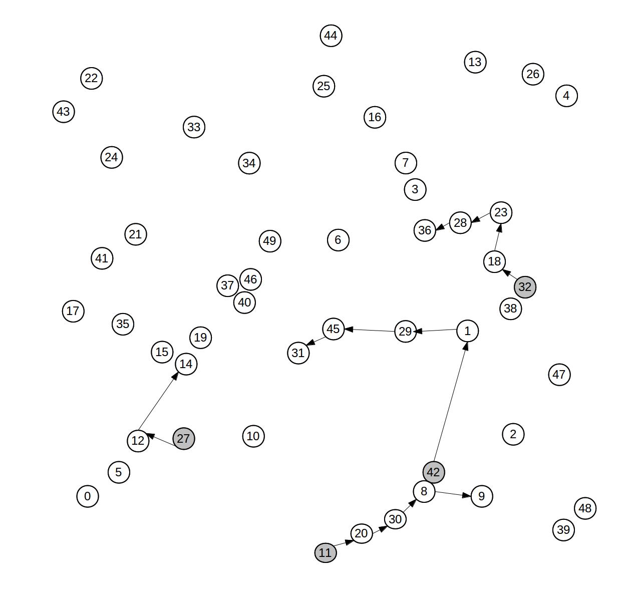
Figure 5: Illustrative random wireless scenario.

For the purposes of the evaluation process, ten different wireless scenarios are generated. For these scenarios, $50$ nodes are uniformly distributed, over an area of $500$m $\times$ $500$m. The number of flows generated, along with the source and destination node for each flow, are selected randomly. A maximum number of ten flows is allowed for each scenario and the simulation time is $20.000$ slots. Traffic sources generate UDP unicast flows and are kept backlogged for the whole simulation period.

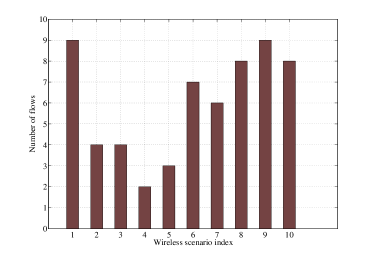
Figure 6: Number of flows per wireless scenario.

Fig. 6, presents the number of flows generated, for each one of the ten wireless scenarios employed. Fig. 5, depicts one such wireless scenario, including four flows. The source and destination nodes for flow $f_{1}$, are $42$ and $31$, respectively. The corresponding source and destination nodes for flows $f_{2}$, $f_{3}$, and $f_{4}$, are: $(11,9)$, $(32,36)$, and $(27,14)$. Before employing the suggested flow allocation scheme, for determining the flow that should be assigned on each path, multiple node-disjoint paths need to be identified, one for each flow. As also shown in this figure, the paths employed for these flows are: $r_{1}:42\rightarrow 1\rightarrow 29\rightarrow 45\rightarrow 31$, $r_{2}:11\rightarrow 20\rightarrow 30\rightarrow 8\rightarrow 9$, $r_{3}:32\rightarrow 18\rightarrow 23\rightarrow 28\rightarrow 36$, and $r_{4}:27\rightarrow 12\rightarrow 14$. Note that the output of the TOFRA scheme is flow rates $q_{42}$, $q_{11}$, $q_{32}$, and $q_{27}$, that will provide with the maximum average aggregate throughput, while also guaranteeing bounded packet delay. In order to capture the effect of interference on success probability and thus, on throughput, different $\gamma$ values are considered. The corresponding values are $0.5,1.0,1.5$, and $2.0$, respectively.

IV-B Simulation Results

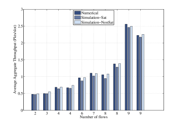
Figure 7: Average Aggregate Throughput: Numerical vs. Simulation results for $\gamma$ $=$ $0.5$.

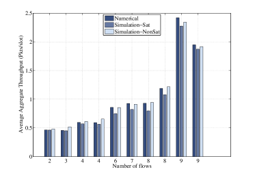
Figure 8: Average Aggregate Throughput: Numerical vs. Simulation results for $\gamma$ $=$ $1.0$.

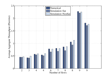
Figure 9: Average Aggregate Throughput: Numerical vs. Simulation results for $\gamma$ $=$ $1.5$.

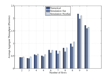
Figure 10: Average Aggregate Throughput: Numerical vs. Simulation results for $\gamma$ $=$ $2.0$.

The evaluation process consists of three parts. In the first one, we explore whether the model employed by the proposed flow allocation scheme (TOFRA), accurately captures the average aggregate throughput (AAT) observed in the simulated scenarios. To introduce the notation used in the figures below, simulation results for the TOFRA variant that is simulated assuming saturated queues, are labelled as Simulation-Sat. Simulation results for the TOFRA variant where the assumption of saturated queues is removed, are labelled as Simulation-NonSat.

Figs. 7 to 10, compare numerical with simulation results, concerning AAT, for SINR threshold values $0.5$, $1.0$, $1.5$, and $2.0$ and the ten different wireless scenarios explored. Simulated results for both TOFRA variants are presented. For the case of the TOFRA variant, where queues for relay nodes are kept backlogged for the whole simulation period, the average deviation over all simulated scenarios, between the numerical and simulation results, is $5.5\%$, $7.6\%$, $9.0\%$, and $10.9\%$, respectively, for the four SINR threshold values considered. In all the scenarios and for all the $\gamma$ values considered, the model employed by the TOFRA scheme overestimates the AAT observed in the simulation results. There are two reasons for this overestimation. The first one, is related to the maximum retransmit threshold. In the analysis employed, its effect is disregarded and thus, no packet is dropped after exceeding a certain number of failed retransmissions. In the simulated results however, it is set to $3.0$, which means that a packet that is unsuccessfully transmitted for three times, it will be dropped. If there is no other packet available in the transmitter’s queue, a dummy packet will be inserted (in case where TOFRA is simulated with the saturated queues assumption) instead. Dummy packets however, are not taken into account for AAT calculation. More on the effect of maximum retransmit threshold on TOFRA’s AAT, consider scenario, $8$ with $\gamma=1.0$, as an example. Simulated AAT for the proposed scheme, when queues are saturated and the maximum retransmit threshold is $3$, is $16.6\%$ lower than the corresponding numerical value. When the corresponding scenario is simulated with an infinite value for the maximum retransmit threshold, the corresponding deviation between numerical and simulated AAT drops to $1.9\%$. The second reason, for the overestimation of the AAT observed in the simulated scenarios is the following: in the analysis, it is assumed that whenever a packet is transmitted it is a packet carrying data. In the simulated scenarios however, all nodes either perform periodic emission of routing protocol’s control messages, or forward received control packets. This means that, specific slots are spent carrying routing protocol’s control messages, instead of data packets, resulting in our analysis overestimating the AAT observed in the simulated results. The second reason for AAT overestimation though, is less important due to the large intervals over which control packets are generated and the small number of nodes participating in the multipath set.

Figs. 7 to 10, also compare the AAT achieved by TOFRA model and the simulated one, when the assumption of saturated queues at the relays is removed. There are three reasons that shape the gap between the numerical and the simulated AAT for TOFRA, when queues are not saturated, with all three reasons stemming from analysis’ assumptions. The first two reasons were described in the previous paragraph and result in our analysis overestimating the AAT observed in the simulated results. The third reason has an opposite effect on AAT and is related to the saturated queues assumption present in the analysis. According to this assumption, whenever a relay node attempts to transmit a packet there is always one available for transmission in its queue. In the simulated scenarios however, this is not always the case. As a result, the actual interference experienced by transmissions along a link, is lower than the one assumed in the analysis and thus, the actual average throughput for a link may be higher than the one calculated by the analysis applied. The effect of this is that, the model employed may underestimate the average throughput of a specific links and thus, may underestimate the AAT. For each $\gamma$ value employed, the average deviation between numerical and simulated results, concerning AAT, is estimated over all ten traffic scenarios explored. The corresponding average deviation values are $3.1\%$, $3.7\%$, $4.0\%$, and $4.7\%$, for $\gamma=0.5,1.0,1.5,2.0$, respectively. Note that, for each wireless scenario, the absolute value of the deviation of simulated from numerical AAT is considered. It is interesting to note that, the deviation between numerical and simulated results, concerning AAT, is lower for the case where the assumption of saturated queues is removed. This is however, due to the contradictory effects on AAT, between the assumption of saturated queues and the assumptions concerning the maximum retransmit threshold, and the occupation of certain slots by routing protocol’s control traffic.

For the rest of the evaluation process, only queues of flow originators will be kept backlogged for the whole simulation period. Queues for relay nodes may be empty during a specific slot. Finally, the minimum and maximum AAT variance value, over all traffic scenarios explored and the four $\gamma$ values considered, are $10^{-4}$ and $10^{-3}$, respectively.

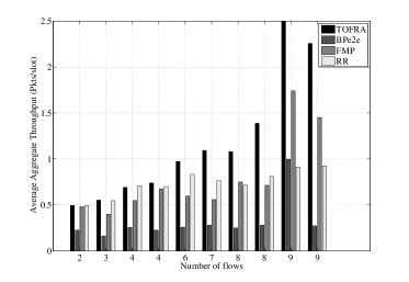
Figure 11: Simulation results: AAT for TOFRA, FMP, BP, and RR for $\gamma$ $=$ $0.5$.

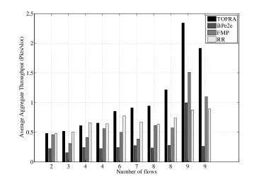
Figure 12: Simulation results: AAT for TOFRA, FMP, BP, and RR for $\gamma$ $=$ $1.0$.

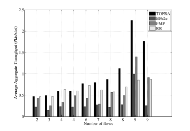
Figure 13: Simulation results: AAT for TOFRA, FMP, BP, and RR for $\gamma$ $=$ $1.5$.

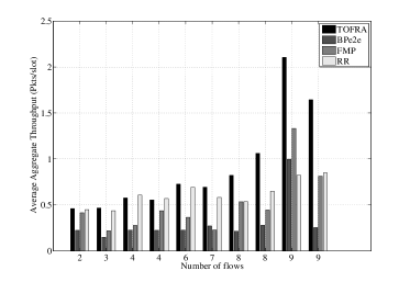
Figure 14: Simulation results: AAT for TOFRA, FMP, BP, and RR for $\gamma$ $=$ $2.0$.

In the second part of the evaluation process, the proposed flow allocation scheme (TOFRA) is compared, in terms of AAT, with three other flow allocation schemes, namely, Best-Path (BP), Full MultiPath (FMP), and Round-Robin (RR). BP employs a single path to the destination, which is the one that exhibits the highest end-to-end success probability (defined in Section III-B) and estimates the flow that should be assigned on this path, by solving a single path version of the flow allocation optimization problem. FMP assigns a flow rate of one packet per slot on each path, while RR employs a different path each time slot. For the evaluation process, we consider the simulated variant for each scheme, where the assumption of saturated queues is removed.

Figs. 11-14, collate the AAT achieved by all aforementioned schemes, for the ten random scenarios employed. Each figure corresponds to one of the different SINR threshold values considered ($0.5$, $1.0$, $1.5$, and $2.0$). As these figures show, the proposed flow allocation scheme (TOFRA) achieves significantly higher ATT than FMP. The main reason for this is that, it takes into account the effect of both intra- and inter-path interference on throughput. FMP on the other hand, assigns the maximum flow data rate on each path (one packet per slot), disregarding the effect of interference. TOFRA achieves $47.3\%$, $63.7\%$, $78.9\%$, and $91.5\%$ higher AAT, on average, over all ten scenarios, than FMP, for $\gamma=0.5,1.0,1.5,2.0$, respectively. The proposed scheme also outer-performs BP, for all traffic scenarios and $\gamma$ values. This is however expected, since TOFRA exploits the diversity among the available paths and is able to aggregate resources from different paths on and interference-aware manner. The average gain of TOFRA over BP is $293.7\%$, $256.4\%$, $2391.1\%$, and $222.1\%$, for the four $\gamma$ values considered.

As far as round robin (RR) scheme is concerned, the average gain of TOFRA over RR, in terms of AAT, is $50.5\%$, $43.7\%$, $41.7\%$, and $39.1\%$, for $\gamma=0.5,1.0,1.5,2.0$, respectively. Comparing TOFRA with RR reveals the following trend: in scenarios where a low number of flows is present ($\leq 4$), the gain of TOFRA over RR is insignificant. Moreover, in specific scenarios, and especially when a larger $\gamma$ value is employed, RR achieves slightly higher AAT than TOFRA. This is the case for scenario $2$ and all $\gamma$ values, and scenario $3$ and $\gamma$ values $1.5$, and $2.0$, respectively. In scenarios with a larger number of flows, TOFRA outer-performs RR. The advantage of RR over TOFRA is that, alternating among the available paths, on an iterative manner, it reduces both inter-path interference and packet failures along each path, due to half-duplex node operation. However, round-robin based flow allocation is expected to exhibit poor performance in two cases: firstly, in scenarios where a larger number of flows is present and thus, a larger number of paths is utilized. In a scenario with $K$ flows, employing $K$ paths for example, each path will remain idle before being assigned another packet to forward, for $K-1$ slots. Secondly, RR is expected to achieve significantly lower AAT than TOFRA in scenarios where there is a large degree of diversity among the available paths. The reason for this is that, RR assigns packets on paths on a periodic manner, without adjusting flow rate based on their quality.

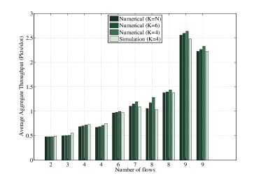
Figure 15: Effect of number of dominant interferers on average aggregate throughput accuracy for $\gamma$ $=$ $0.5$.

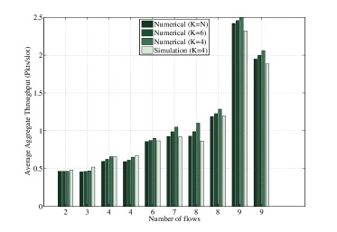
Figure 16: Effect of number of dominant interferers on average aggregate throughput accuracy for $\gamma$ $=$ $1.0$.

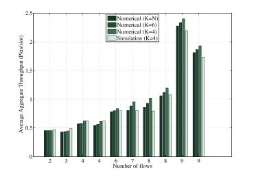
Figure 17: Effect of number of dominant interferers on average aggregate throughput accuracy for $\gamma$ $=$ $1.5$.

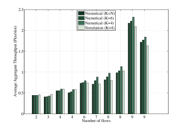
Figure 18: Effect of number of dominant interferers on average aggregate throughput accuracy for $\gamma$ $=$ $2.0$.

In the last part of the evaluation process, a variant of the proposed scheme is explored, where interference is approximated by considering only the dominant interfering nodes for each link. The goal is to reduce the complexity of expressing the average aggregate throughput (AAT) achieved by all flows and consequently, of solving the flow allocation optimization problem. As already described in Section III-A, the first step of the process for formulating flow allocation as an optimization problem, is deriving the expression for a link’s average throughput. Instead of considering all possible interfering nodes for expressing the average throughput achieved over that link, the interference imposed on it, is approximated by taking into account only the k dominant ones. The term dominant interfering nodes refers to transmitters that contribute with the most significant amount of interference, on average, to packet receptions over a specific link and thus, have the most significant effect on its success probability. Approximating the interference imposed on a link in this way, under-estimates the actual interference experienced by that link in the simulated scenarios, and thus, results in an over-estimation of the AAT.

The purpose of this part of the evaluation process is to explore the trade-off between, reduced complexity in formulating flow allocation as an optimization problem and accuracy in capturing the average aggregate throughput observed in the simulated scenarios. For each wireless scenario and $\gamma$ value ($0.5$, $1.0$, $1.5$, and $2.0$), the flow allocation problem employed by the TOFRA scheme, is formulated and solved through the simulated annealing technique, considering each time a different number of dominant interfering nodes ($K=2,...,6$). In this way, the proposed scheme estimates the rates that achieve maximum AAT, along with the corresponding AAT value, for each wireless scenario, $\gamma$ value, and different number of interfering nodes. Numerical results concerning AAT that are estimated on this way are presented in Figs. 15-18, with labels Numerical (K=N), Numerical (K=6), and Numerical (K=4), based on the number of dominant interfering nodes considered. Note that, label Numerical (K=N), indicates numerical results derived by the flow allocation optimization problem, by considering all interfering nodes for each link.

When the number of interfering nodes considered, for expressing each link’s average throughput is reduced, TOFRA overestimates the maximum AAT that can be achieved, by all flows present in the wireless scenario considered. Comparing numerical results concerning TOFRA’s AAT, for $K=N$, and $K=6$, the average overestimation over all wireless scenarios is $2.6\%$, $3.0\%$, $3.6\%$, and $3.9\%$, for $\gamma=0.5,1.0,1.5,$ and $2.0$, respectively. The corresponding values, for the case where numerical results for $K=N$, and $K=4$ are compared, are $5.7\%$, $7.7\%$, $9.4\%$, and $10.8\%$. As Figs. 15-18 also show, this overestimation becomes more significant for large $\gamma$ values, where the effect of interference on success probability becomes more acute. These results show that, considering only a small number of dominant interfering nodes for each link, results in TOFRA estimating an AAT value, that differs insignificantly from the one estimated when all interfering nodes are taken into account.

What is most interesting though, is to explore whether the AAT estimated through TOFRA’s model, when considering only the $K$ dominant interfering nodes for each link, differs significantly from the actual AAT observed in the simulated scenarios. It is also important to note that, while estimating the received SINR for a specific packet, all active transmitters are taken into account for interference inference, implying that, the actual interference experienced by a link in the simulated scenarios, is higher than the one considered by the TOFRA variant, where interference for each link is approximated by considering the dominant interfering nodes only.

Observing Figs. 15-18 shows that, for all $\gamma$ values and for most scenarios, TOFRA’s AAT, in the simulated scenarios, is lower than the one estimated by the analysis employed (flow allocation optimization problem). This is expected however, since in the analysis, only a subset of all the interfering nodes (the dominant ones) are considering for expressing a specific link’s average throughput. To be more precise, TOFRA’s AAT observed in the simulated scenarios, is lower than the corresponding numerical values for $60\%$ of the wireless scenarios, for $\gamma=0.5,1.0,1.5,$ and for $70\%$ of them for $\gamma=2.0$. It is also interesting to note that, in some scenarios, the simulated AAT is higher than the one estimated by the flow allocation optimization problem. The reason for this, was also discussed in the first part of the evaluation process, in the beginning of this section, and is related to the saturated queues assumption present in our analysis. Even if only the dominant interfering nodes are considered for a specific link, it is assumed that these nodes will always have a packet available for transmission in their queues. However, this is not always the case in the simulated scenarios and so, the actual interference experienced by a link, from these dominant interferers, may be lower than the one estimated by our analysis. In this way, the effect of interference underestimation, by considering only the dominant interfering nodes for each link, is counter-balanced. For each wireless scenario and $\gamma$ value, the absolute value of the deviation between numerical and simulated AAT is estimated, for the case, where both of them are derived by considering only the four dominant interfering nodes for each link. The average value of this deviation, over all wireless scenarios, is $6.8\%$, $8.5\%$, $9.6\%$, and $9.6\%$, for $\gamma=0.5,1.0,1.5,$ and $2.0$ respectively. These results show that, the gain of reduced complexity for expressing a link’s average throughput, comes at an insignificant cost in the accuracy with which simulated AAT for the proposed scheme is captured by the analysis employed.

V Conclusion

This study, explores the issue of aggregate throughput optimal flow rate allocation, for wireless, multi-hop, random access networks, with multi-packet reception capabilities. Flows are forwarded over multiple node disjoint paths, experiencing both intra- and inter-path interference. We propose a distributed scheme that formulates flow rate allocation as an optimization problem, aimed at maximizing the average aggregate throughput of all flows, while also providing bounded packet delay guarantees. The key feature of the suggested scheme is that, it employs a simple model for the average aggregate throughput, that captures both intra- and inter-path interference through the SINR model. A simple topology is employed to demonstrate the proposed scheme and also show that the corresponding optimization problem is non-convex. We evaluate the suggested flow allocation scheme using Ns2 simulations of ten random wireless scenarios. Collating numerical with simulations results reveals that, the suggested scheme accurately captures the average aggregate throughput observed in the simulated scenarios, despite the simplifying assumptions adopted by our analysis. Moreover, it achieves significantly higher average aggregate throughput than best-path, full multipath and a round-robin based flow allocation scheme. As part of the evaluation process, we also explore the trade-off between, reduced complexity in formulating flow allocation as an optimization problem and the accuracy in estimating the average aggregate throughput observed in the simulation results. A variant of the proposed scheme is explored, where interference for each link is approximated by considering the dominant interfering nodes only for expressing its average throughput. Simulation results show that, approximating the interference experienced by each link by considering only the dominant interfering nodes, results in an insignificant deviation between numerical and simulation results, regarding AAT.

Part of our future work, is to address fairness issues too, apart from maximizing the aggregate throughput achieved by all flows. We also plan to consider multiple transmission rates and relax the assumption of fixed transmission probability per relay, by allowing a variable contention window. In the present study we treat interference as noise. In future steps, we aim at adopting more sophisticated approaches for interference handling, such as, successive interference cancellation and joint decoding [34, 38]. Finally, we aim at exploring the performance of the suggested flow rate allocation scheme under the assumption of bursty packet losses.

References

- [1] M. Ploumidis, N. Pappas, and A. Traganitis, “Throughput optimal flow allocation on multiple paths for random access wireless multi-hop networks,” in IEEE Globecom Workshops (GC Wkshps), pp. 263–268, Dec. 2013.
- [2] L. Le, “Multipath routing design for wireless mesh networks,” in IEEE Global Telecommunications Conference (GLOBECOM), pp. 1–6, Dec. 2011.
- [3] N. Pappas, V. A. Siris, and A. Traganitis, “Path diversity gain with network coding and multipath transmission in wireless mesh networks,” in IEEE International Symposium on a World of Wireless Mobile and Multimedia Networks (WoWMoM), pp. 1–6, June 2010.
- [4] M. Ploumidis, N. Pappas, V. A. Siris, and A. Traganitis, “On the performance of network coding and forwarding schemes with different degrees of redundancy for wireless mesh networks,” Computer Communications, vol. 72, pp. 49 – 62, 2015.
- [5] J. Tsai and T. Moors, “Interference-aware multipath selection for reliable routing in wireless mesh networks,” in IEEE Internatonal Conference on Mobile Adhoc and Sensor Systems (MASS), pp. 1–6, Oct. 2007.
- [6] R. Leung, J. Liu, E. Poon, A.-L. Chan, and B. Li, “Mp-dsr: a qos-aware multi-path dynamic source routing protocol for wireless ad-hoc networks,” in 26th Annual IEEE Conference on Local Computer Networks, pp. 132–141, 2001.
- [7] Z. Wang, E. Bulut, and B. Szymanski, “Energy efficient collision aware multipath routing for wireless sensor networks,” in IEEE International Conference on Communications (ICC), pp. 1–5, June 2009.
- [8] M. S. Siddiqui, S. O. Amin, J. H. Kim, and C. S. Hong, “Mhrp: A secure multi-path hybrid routing protocol for wireless mesh network,” in IEEE Military Communications Conference (MILCOM), pp. 1–7, Oct. 2007.
- [9] J. Chen, S. He, Y. Sun, P. Thulasiraman, and X. Shen, “Optimal flow control for utility-lifetime tradeoff in wireless sensor networks,” in IEEE Global Telecommunications Conference (GLOBECOM), pp. 1–6, Dec. 2009.
- [10] A. Valera, W. Seah, and S. Rao, “Cooperative packet caching and shortest multipath routing in mobile ad hoc networks,” in The 22nd IEEE Conference of the Computer and Communications (INFOCOM), vol. 1, pp. 260–269, Mar. 2003.
- [11] V. Sharma, S. Kalyanaraman, K. Kar, K. Ramakrishnan, and V. Subramanian, “Mplot: A transport protocol exploiting multipath diversity using erasure codes,” in The 27th IEEE Conference on Computer Communications (INFOCOM), pp. 121–125, April 2008.
- [12] M. Alicherry, R. Bhatia, and L. E. Li, “Joint channel assignment and routing for throughput optimization in multiradio wireless mesh networks,” IEEE Journal on Selected Areas in Communications (JSAC), vol. 24, pp. 1960–1971, Nov. 2006.
- [13] G. Middleton, B. Aazhang, and J. Lilleberg, “Efficient resource allocation and interference management for streaming multiflow wireless networks,” in IEEE International Conference on Communications (ICC), pp. 1–5, May 2010.
- [14] G. Middleton, B. Aazhang, and J. Lilleberg, “A flexible framework for polynomial-time resource allocation in streaming multiflow wireless networks,” IEEE Transactions on Wireless Communications, vol. 11, pp. 952–963, Mar. 2012.
- [15] X. Lin and N. Shroff, “Joint rate control and scheduling in multihop wireless networks,” in IEEE Conference on Decision and Control (CDC), vol. 2, pp. 1484–1489, Dec. 2004.
- [16] U. Akyol, M. Andrews, P. Gupta, J. Hobby, I. Saniee, and A. Stolyar, “Joint scheduling and congestion control in mobile ad-hoc networks,” in The 27th IEEE Conference on Computer Communications (INFOCOM), pp. 619–627, Apr. 2008.
- [17] L. Chen, S. Low, M. Chiang, and J. Doyle, “Cross-layer congestion control, routing and scheduling design in ad hoc wireless networks,” in The 25th IEEE International Conference on Computer Communications (INFOCOM), pp. 1–13, Apr. 2006.
- [18] Q. Gao, J. Zhang, and S. Hanly, “Cross-layer rate control in wireless networks with lossy links: leaky-pipe flow, effective network utility maximization and hop-by-hop algorithms,” IEEE Transactions on Wireless Communications, vol. 8, pp. 3068–3076, Jun. 2009.
- [19] Y. Yu and G. Giannakis, “Cross-layer congestion and contention control for wireless ad hoc networks,” IEEE Transactions on Wireless Communications, vol. 7, pp. 37–42, Jan. 2008.
- [20] X. Wang and K. Kar, “Cross-layer rate optimization for proportional fairness in multihop wireless networks with random access,” IEEE Journal on Selected Areas in Communications (JSAC), vol. 24, pp. 1548–1559, Aug. 2006.
- [21] M. Uddin, C. Rosenberg, W. Zhuang, and A. Girard, “Joint configuration of routing and medium access parameters in wireless networks,” in IEEE Global Telecommunications Conference (GLOBECOM), pp. 1–8, Nov. 2009.
- [22] S. Avallone and G. Di Stasi, “A new mpls-based forwarding paradigm for multi-radio wireless mesh networks,” IEEE Transactions on Wireless Communications, vol. 12, pp. 3968–3979, Aug. 2013.
- [23] G. D. Stasi, J. Karlsson, S. Avallone, R. Canonico, A. Kassler, and A. Brunstrom, “Combining multi-path forwarding and packet aggregation for improved network performance in wireless mesh networks,” Computer Networks, vol. 64, no. 0, pp. 26 – 37, 2014.
- [24] X. Zhu and B. Girod, “Distributed rate allocation for multi-stream video transmission over ad hoc networks,” in IEEE International Conference on Image Processing (ICIP), vol. 2, pp. 157–160, Sep. 2005.
- [25] X. L. Huang and B. Bensaou, “On max-min fairness and scheduling in wireless ad-hoc networks: Analytical framework and implementation,” in ACM International Symposium on Mobile Ad Hoc Networking and Computing (MobiHoc), pp. 221–231, 2001.
- [26] V. Srinivasan, C. Chiasserini, P. Nuggehalli, and R. Rao, “Optimal rate allocation for energy-efficient multipath routing in wireless ad hoc networks,” IEEE Transactions on Wireless Communications, vol. 3, pp. 891–899, May 2004.
- [27] B. Radunović, C. Gkantsidis, D. Gunawardena, and P. Key, “Horizon: balancing tcp over multiple paths in wireless mesh network,” in ACM international conference on Mobile computing and networking (MobiCom), pp. 247–258, 2008.
- [28] C. Gkantsidis, W. Hu, P. Key, B. Radunovic, P. Rodriguez, and S. Gheorghiu, “Multipath code casting for wireless mesh networks,” in ACM CoNEXT Conference (CoNEXT), pp. 10:1–10:12, 2007.
- [29] B. Radunovic, C. Gkantsidis, P. Key, and P. Rodriguez, “An optimization framework for opportunistic multipath routing in wireless mesh networks,” in The 27th IEEE Conference on Computer Communications (INFOCOM), Apr. 2008.
- [30] N. Pappas, M. Kountouris, A. Ephremides, and A. Traganitis, “Relay-assisted multiple access with full-duplex multi-packet reception,” IEEE Transactions on Wireless Communications, vol. 14, pp. 3544–3558, July 2015.
- [31] N. Pappas, A. Ephremides, and A. Traganitis, “Relay-assisted multiple access with multi-packet reception capability and simultaneous transmission and reception,” in IEEE Information Theory Workshop (ITW), pp. 578–582, Oct 2011.
- [32] G. Papadimitriou, N. Pappas, A. Traganitis, and V. Angelakis, “Network-level performance evaluation of a two-relay cooperative random access wireless system,” Computer Networks, vol. 88, pp. 187 – 201, 2015.
- [33] S. Verdu, Multiuser Detection. Cambridge University Press, 1st ed., 1998.
- [34] D. Tse and P. Viswanath, Fundamentals of wireless communication. Cambridge University Press, 2005.
- [35] G. Nguyen, S. Kompella, J. Wieselthier, and A. Ephremides, “Optimization of transmission schedules in capture-based wireless networks,” in IEEE Military Communications Conference (MILCOM), pp. 1–7, Nov. 2008.
- [36] “The Network Simulator NS-2.” http://www.isi.edu/nsnam/ns/.
- [37] F. J. Ros, “Um-olsr.” http://masimum.dif.um.es/?Software:UM-OLSR.
- [38] M. Ploumidis, N. Pappas, and A. Traganitis, “Performance of flow allocation with successive interference cancelation for random access wmns,” in IEEE Globecom Workshops (GC Wkshps), pp. 1–7, Dec 2015.