Discrete Family Symmetry from F-Theory GUTs

Athanasios Karozas^† , Stephen F. King^⋆ , George K. Leontaris^† , Andrew K. Meadowcroft^⋆

^⋆ School of Physics and Astronomy, University of Southampton,

SO17 1BJ Southampton, United Kingdom

^† Physics Department, Theory Division, Ioannina University,

GR-45110 Ioannina, Greece

We consider realistic F-theory GUT models based on discrete family symmetries $A_{4}$ and $S_{3}$, combined with $SU(5)$ GUT, comparing our results to existing field theory models based on these groups. We provide an explicit calculation to support the emergence of the family symmetry from the discrete monodromies arising in F-theory. We work within the spectral cover picture where in the present context the discrete symmetries are associated to monodromies among the roots of a five degree polynomial and hence constitute a subgroup of the $S_{5}$ permutation symmetry. We focus on the cases of $A_{4}$ and $S_{3}$ subgroups, motivated by successful phenomenological models interpreting the fermion mass hierarchy and in particular the neutrino data. More precisely, we study the implications on the effective field theories by analysing the relevant discriminants and the topological properties of the polynomial coefficients, while we propose a discrete version of the doublet-triplet splitting mechanism.

1 Introduction

F-theory is defined on an elliptically fibered Calabi-Yau four-fold over a threefold base [1]. In the elliptic fibration the singularities of the internal manifold are associated to the gauge symmetry. The basic objects in these constructions are the D7-branes which are located at the “points” where the fibre degenerates, while matter fields appear at their intersections. The interesting fact in this picture is that the topological properties of the internal space are converted to constraints on the effective field theory model in a direct manner. Moreover, in these constructions it is possible to implement a flux mechanism which breaks the symmetry and generates chirality in the spectrum.

F-theory Grand Unified Theories (F-GUTs) [2, 3, 4, 5, 6, 7, 8] represent a promising framework for addressing the flavour problem of quarks and leptons (for reviews see [9, 10, 11, 12, 13, 14]). F-GUTs are associated with D7-branes wrapping a complex surface $S$ in an elliptically fibered eight dimensional internal space. The precise gauge group is determined by the specific structure of the singular fibres over the compact surface $S$, which is strongly constrained by the Kodaira conditions. The so-called “semi-local” approach imposes constraints from requiring that S is embedded into a local Calabi-Yau four-fold, which in practice leads to the presence of a local $E_{8}$ singularity [15], which is the highest non-Abelian symmetry allowed by the elliptic fibration.

In the convenient Higgs bundle picture and in particular the spectral cover approach, one may work locally by picking up a subgroup of $E_{8}$ as the gauge group of the four-dimensional effective model while the commutant of it with respect to $E_{8}$ is associated to the geometrical properities in the vicinity. Monodromy actions, which are always present in F-theory constructions, may reduce the rank of the latter, leaving intact only a subgroup of it. The remaining symmetries could be $U(1)$ factors in the Cartan subalgebra or some discrete symmetry. Therefore, in these constructions GUTs are always accompanied by additional symmetries which play important role in low energy pheomenology through the restrictions they impose on superpotential couplings.

In the above approach, all Yukawa couplings originate from this single point of $E_{8}$ enhancement. As such, we can learn about the matter and couplings of the semi-local theory by decomposing the adjoint of $E_{8}$ in terms of representations of the GUT group and the perpendicular gauge group. In terms of the local picture considered so far, matter is localised on curves where the GUT brane intersects other 7-branes with extra $U(1)$ symmetries associated to them, with this matter transforming in bi-fundamental representations of the GUT group and the $U(1)$. Yukawa couplings are then induced at points where three matter curves intersect, corresponding to a further enhancement of the gauge group.

Since $E_{8}$ is the highest symmetry of the elliptic fibration, the gauge symmetry of the effective model can in principle be any of the $E_{8}$ subgroups. The gauge symmetry can be broken by turning on appropriate fluxes [16] which at the same time generate chirality for matter fields. The minimal scenario of $SU(5)$ GUT has been extensively studied  [17, 18, 19]. Indeed only the simplest $SU(5)$ GUTs can in principle avoid exotic matter in the spectrum [4]. However, by considering different fluxes, other models have been constructed with different GUT groups, such as $SO(10)$ and $E_{6}$ [20, 21, 22, 23, 24]. In particular, it is possible to achieve gauge coupling unification from $E_{6}$ in the presence of TeV scale exotics originating from both the matter curves and the bulk [25].

All of the approaches mentioned so far exploit the extra $U(1)$ symmetries as family symmetries, in order to address the quark and lepton mass hierarchies. While it is gratifying that such symmetries can arise from a string derived model, where the parameter space is subject to constraints from the first principles of the theory, the possibility of having only continuous Abelian family symmetry in F-theory represents a very restrictive choice. By contrast, other string theories have a rich group structure embodying both continuous as well as discrete symmetries at the same time [26]-[31]. It may be regarded as something of a drawback of the F-theory approach that the family symmetry is constrained to be a product of $U(1)$ symmetries. Indeed the results of the neutrino oscillation experiments are in agreement with an almost maximal atmospheric mixing angle $\theta_{23}$, a large solar mixing $\theta_{12}$, and a non-vanishing but smaller reactor angle $\theta_{13}$, all of which could be explained by an underlying non-Abelian discrete family symmetry (for recent reviews see for example [32, 33, 34]).

Recently, discrete symmetries in F-theory have been considered [35] on an elliptically fibered space with an $SU(5)$ GUT singularity, where the effective theory is invariant under a more general non-Abelian finite group. They considered all possible monodromies which induce an additional discrete (family-type) symmetry on the model. For the $SU(5)$ GUT minimal unification scenario in particular, the accompanying discrete family group could be any subgroup of the $S_{5}$ permutation symmetry, and the spectral cover geometries with monodromies associated to the finite symmetries $S_{4}$, $A_{4}$ and their transitive subgroups, including the dihedral group $D_{4}$ and $Z_{2}\times Z_{2}$, were discussed. However a detailed analysis was only presented for the $Z_{2}\times Z_{2}$ case, while other cases such as $A_{4}$ were not fully developed into a realistic model.

In this paper we extend the analysis in [35] in order to construct realistic models based on the cases $A_{4}$ and $S_{3}$, combined with $SU(5)$ GUT, comparing our results to existing field theory models based on these groups. We provide an explicit calculation to support the emergence of the family symmetry as from the discrete monodromies. In section 2 we start with a short description of the basic ingredients of F-theory model building and present the splitting of the spectral cover in the components associated to the $S_{4}$ and $S_{3}$ discrete group factors. In section 3 we discuss the conditions for the transition of $S_{4}$ to $A_{4}$ discrete family symmetry “escorting” the $SU(5)$ GUT and propose a discrete version of the doublet-triplet splitting mechanism for $A_{4}$, before constructing a realistic model which is analysed in detail. In section 4 we then analyse in detail an $S_{3}$ model which was not considered at all in  [35] and in section 5 we present our conclusions. Additional computational details are left for the Appendices.

2 General Principles

F-theory is a non-perturbative formulation of type IIB superstring theory, emerging from compactifications on a Calabi-Yau fourfold which is an elliptically fibered space over a base $B_{3}$ of three complex dimensions. Our GUT symmetry in the present work is $SU(5)$ which is associated to a holomorphic divisor residing inside the threefold base, $B_{3}$. If we designate with $z$ the ‘normal’ direction to this GUT surface, the divisor can be thought of as the zero limit of the holomorphic section $z$ in $B_{3}$, i.e. at $z\to 0$. The fibration is described by the Weierstrass equation

$$y^{2}=x^{3}+f(z)x+g(z)\,,$$

where $f(z),g(z)$ are eighth and twelveth degree polynomials respectively. The singularities of the fiber are determined by the zeroes of the discriminant $\Delta=4f^{3}+27g^{2}$ and are associated to non-Abelian gauge groups. For a smooth Weierstrass model they have been classified by Kodaira and in the case of F-theory these have been used to describe the non-Abelian gauge group. Under these conditions, the highest symmetry in the elliptic fibration is $E_{8}$ and since the GUT symmetry in the present work is chosen to be $SU(5)$, its commutant is $SU(5)_{\perp}$. The physics of the latter is nicely captured by the spectral cover, described by a five-degree polynomial

$$\begin{split}{\cal C}_{5}:&\qquad\sum_{k=0}^{5}b_{k}s^{5-k}=0\,,\end{split}$$ (1)

where $b_{k}$ are holomorphic sections and $s$ is an affine parameter. Under the action of certain fluxes and possible monodromies, the polynomial could in principle be factorised to a number of irreducible components

$${\cal C}_{5}\to C_{a_{1}}\times\cdots\times C_{a_{n}},\;1+\cdots+n<5$$

provided that new coefficients preserve the holomorphicity. Given the rank of the associated group ($SU(5)_{\perp}$), the simplest possibility is the decomposition into four $U(1)$ factors, but this is one among many possibilities. As a matter of fact, in an F-theory context, the roots of the spectral cover equation are related by non-trivial monodromies. For the $SU(5)_{\perp}$ case at hand, under specific circumstances (related mainly to the properties of the internal manifold and flux data) these monodromies can be described by any possible subgroup of the Weyl group $S_{5}$. This has tremendous implications in the effective field theory model, particularly in the superpotential couplings. The spectral cover equation (1) has roots $t_{i}$, which correspond to the weights of $SU(5)_{\perp}$, i.e. $b_{0}\prod_{i=1}^{5}(s-t_{i})=0$. The equation describes the matter curves of a particular theory, with roots being related by monodromies depending on the factorisation of this equation. Thus, we may choose to assume that the spectral cover can be factorised, with new coefficients $a_{j}$ that lie within the same field ${\cal F}$ as $b_{i}$. Depending on how we factorise, we will see different monodromy groups. Motivated by the peculiar properties of the neutrino sector, here we will attempt to explore the low energy implications of the following factorisations of the spectral cover equation

$$i)\;{\cal C}_{4}\times{\cal C}_{1},\;\;ii)\;{\cal C}_{3}\times{\cal C}_{2},\;\;iii)\;{\cal C}_{3}\times{\cal C}_{1}\times{\cal C}_{1}\,.$$ (2)

Case $i)$ involves the transitive group $S_{4}$ and its subgroups $A_{4}andD_{4}$ while cases $ii)$ and $iii)$ incorporate the $S_{3}$, which is isomorphic to $D_{3}$. For later convenience these cases are depicted in figure 1.

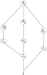
Figure 1: $S_{4}$ and its subgroups relevant to the present analysis.

In case $i)$ for example, the polynomial in equation (1) should be separable in the following two factors

$${\cal C}_{4}\times{\cal C}_{1}:\left(a_{1}+a_{2}s+a_{3}s^{2}+a_{4}s^{3}+a_{5}s^{4}\right)(a_{6}+a_{7}s)=0$$ (3)

which implies the ‘breaking’ of the $SU(5)_{\perp}$ to the monodromy group $S_{4}$, (or one of its subgroups such as $A_{4}$), described by the fourth degree polynomial

$${\cal C}_{4}:\qquad\sum_{k=1}^{5}a_{k}s^{k-1}=0$$ (4)

and a $U(1)$ associated with the linear part. New and old polynomial coefficients satisfy simple relations $b_{k}=b_{k}(a_{i})$ which can be easily extracted comparing same powers of (1) and (3) with respect to the parameter $s$. Table 1 summarizes the relations between the coefficients of the unfactorised spectral cover and the $a_{j}$ coefficients for the cases under consideration in the present work.

The homologies of the coefficients $b_{i}$ are given in terms of the first Chern class of the tangent bundle ($c_{1}$) and of the normal bundle ($-t$),

$$\begin{gathered}\left[b_{k}\right]=\eta-kc_{1}\,,\\ \text{where}\,\,\,\eta=6c_{1}-t\,.\end{gathered}$$ (5)

We may use these to calculate the homologies $\left[a_{j}\right]$ of our $a_{j}$ coefficients, since if $b_{i}=a_{j}a_{k}\dots$ then $\left[b_{i}\right]=\left[a_{j}\right]+\left[a_{k}\right]+\dots$, allowing us to rearrange for the required homologies. Note that since we have in general more $a_{j}$ coefficients than our fully determined $b_{i}$ coefficients, the homologies of the new coefficients cannot be fully determined. For example, if we factorise in a $3+1+1$ arrangement, we must have $3$ unknown parameters, which we call $\chi_{k=1,2,3}$.

$b_{i}$	$a_{j}$ coefficients for 4+1	$a_{j}$ coefficients for 3+2	$a_{j}$ coefficients for 3+1+1
$b_{0}$	$a_{5}a_{7}$	$a_{4}a_{7}$	$a_{4}a_{6}a_{8}$
$b_{1}$	$a_{5}a_{6}+a_{4}a_{7}$	$a_{4}a_{6}+a_{3}a_{7}$	$a_{4}a_{6}a_{7}+a_{4}a_{5}a_{8}+a_{3}a_{6}a_{8}$
$b_{2}$	$a_{4}a_{6}+a_{3}a_{7}$	$a_{4}a_{5}+a_{3}a_{6}+a_{2}a_{7}$	$a_{4}a_{5}a_{7}+a_{3}a_{5}a_{8}+a_{3}a_{6}a_{7}+a_{2}a_{6}a_{8}$
$b_{3}$	$a_{3}a_{6}+a_{2}a_{7}$	$a_{3}a_{5}+a_{2}a_{6}+a_{1}a_{7}$	$a_{3}a_{5}a_{7}+a_{2}a_{5}a_{8}+a_{2}a_{6}a_{7}+a_{1}a_{6}a_{8}$
$b_{4}$	$a_{2}a_{6}+a_{1}a_{7}$	$a_{2}a_{5}+a_{1}a_{6}$	$a_{2}a_{5}a_{7}+a_{1}a_{6}a_{7}+a_{1}a_{5}a_{8}$
$b_{5}$	$a_{1}a_{6}$	$a_{1}a_{5}$	$a_{1}a_{5}a_{7}$

Table 1: table showing the relations $b_{i}=b_{i}(a_{j})$ between coefficients of the spectral cover equation under various decompositions from the unfactorised equation.

In the following sections we will examine in detail the predictions of the $A_{4}$ and $S_{3}$ models.

3 $A_{4}$ models in F-theory

We assume that the spectral cover equation factorises to a quartic polynomial and a linear part, as shown in (3). T he homologies of the new coefficients may be derived from the original $b_{i}$ coefficients. Referring to Table 1, we can see that the homologies for this factorisation are easily calculable, up to some arbitrariness of one of the coefficients - we have seven $a_{j}$ and only six $b_{i}$. We choose $[a_{6}]=\chi$ in order to make this tractable. It can then be shown that the homologies obey:

$$\begin{gathered}\left[a_{i}\right]=\eta-(6-i)c_{1}-\chi\,,\\ \text{Where }i\in\{1,\dots,5\}\\ \left[a_{7}\right]=c_{1}+\chi\\ \left[a_{6}\right]=\chi\,.\end{gathered}$$ (6)

This amounts to asserting that the five of $SU(5)_{\perp}$ ‘breaks’ to a discrete symmetry between four of its weights ($S_{4}$ or one of its subgroups) and a $U(1)_{\perp}$.

The roots of the spectral cover equation must obey:

$$b_{0}\prod_{i=1}^{5}(s-t_{i})=0\,,$$ (7)

where $t_{i}$ are the weights of the five representation of $SU(5)_{\perp}$. When $s=0$, this defines the tenplet matter curves of the $SU(5)_{\text{GUT}}$ [36], with the number of curves being determined by how the result factorises. In the case under consideration, when $s=0$, $b_{5}=0$. After referring to Table 1, we see that this implies that $P_{10}=a_{1}a_{6}=0$. Therefore there are two tenplet matter curves, whose homologies are given by those of $a_{1}$ and $a_{6}$. We shall assume at this point that these are the only two distinct curves, though $a_{1}$ appears to be associated with $S_{4}$ (or a subgroup) and hence should be reducible to a triplet and singlet.

Similarly, for the fiveplets, we have

$$b_{0}\prod_{i=1}^{5}(s-t_{i}-t_{j})=0\,\,\,\,\text{for}\,i\neq j,$$ (8)

which can be shown to give the defining condition for the fiveplets: $P_{5}=b_{4}b_{3}^{2}-b_{2}b_{5}b_{3}+b_{0}b_{5}^{2}=0$. Again consulting the Table 1, we can write this in terms of the $a_{j}$ coefficients:

$$P_{5}=\left(a_{3}a_{6}+a_{2}a_{7}\right)^{2}\left(a_{2}a_{6}a_{1}a_{7}\right)-\left(a_{4}a_{6}+a_{3}a_{7}\right)\left(a_{3}a_{6}+a_{2}a_{7}\right)\left(a_{1}a_{6}\right)+a_{1}^{2}a_{5}a_{6}^{2}a_{7}\,.$$ (9)

Using the condition that $SU(5)$ must be traceless, and hence $b_{1}=0$, we have that $a_{4}a_{7}+a_{5}a_{6}=0$. An Ansatz solution of this condition is $a_{4}=\pm a_{0}a_{6}$ and $a_{5}=\mp a_{0}a_{7}$, where $a_{0}$ is some appropriate scaling with homology $\left[a_{0}\right]=\eta-2(c_{1}+\chi)$, which is trivially derived from the homologies of $a_{4}$ and $a_{6}$ (or indeed $a_{5}$ and $a_{7}$) [35]. If we introduce this, then $P_{5}$ splits into two matter curves:

$$P_{5}=\left(a_{2}^{2}a_{7}+a_{2}a_{3}a_{6}\mp a_{0}a_{1}a_{6}^{2}\right)\left(a_{3}a_{6}^{2}+(a_{2}a_{6}+a_{1}a_{7})a_{7}\right)=0\,.$$ (10)

The homologies of these curves are calculated from those of the $b_{i}$ coefficients and are presented in Table 2. We may also impose flux restrictions if we define:

$$\begin{gathered}{\mathcal{F}}_{Y}\cdot\chi=N\,,\\ {\mathcal{F}}_{Y}\cdot c_{1}={\mathcal{F}}_{Y}\cdot\eta=0\,,\end{gathered}$$ (11)

where $N\in\mathbb{Z}$ and $\mathcal{F}_{Y}$ is the hypercharge flux.

Curve	Equation	Homology	Hyperflux - N	Multiplicity
$10_{a}$	$a_{1}$	$\eta-5c_{1}-\chi$	$-N$	$M_{10_{a}}$
$10_{b}$	$a_{6}$	$\chi$	$+N$	$M_{10_{b}}$
$5_{c}$	$a_{2}^{2}a_{7}+a_{2}a_{3}a_{6}\mp a_{0}a_{1}a_{6}^{2}$	$2\eta-7c_{1}-\chi$	$-N$	$M_{5_{c}}$
$5_{d}$	$a_{3}a_{6}^{2}+(a_{2}a_{6}+a_{1}a_{7})a_{7}$	$\eta-3c_{1}+\chi$	$+N$	$M_{5_{d}}$

Table 2: table of matter curves, their homologies, charges and multiplicities.

Considering equation (7), we see that $b_{5}/b_{0}=t_{1}t_{2}t_{3}t_{4}t_{5}$, so there are at most five ten-curves, one for each of the weights. Under $S_{4}$ and it’s subgroups, four of these are identified, which corroborates with the two matter curves seen in Table 1. As such we identify $t_{i=1,2,3,4}$ with this monodromy group and the coefficient $a_{1}$ and leave $t_{5}$ to be associated to $a_{6}$.

Similarly, equation (8) shows that we have at most ten five-curves when $s=0$, given in the form $t_{i}+t_{j}$ with $i\neq j$. Examining the equations for the two five curves that are manifest in this model after application of our monodromy, the quadruplet involving $t_{i}+t_{5}$ forms the curve labeled $5_{d}$, while the remaining sextet - $t_{i}+t_{j}$ with $i,j\neq 5$ - sits on the $5_{c}$ curve.

3.1 The discriminant

The above considerations apply equally to both the $S_{4}$ as well as $A_{4}$ discrete groups. From the effective model point of view, all the useful information is encoded in the properties of the polynomial coefficients $a_{k}$ and if we wish to distinguish these two models further assumptions for the latter coefficients have to be made. Indeed, if we assume that in the above polynomial, the coefficients belong to a certain field $a_{k}\in{\cal F}$, without imposing any additional specific restrictions on $a_{k}$, the roots exhibit an $S_{4}$ symmetry. If, as desired, the symmetry acting on roots is the subgroup $A_{4}$ the coefficients $a_{k}$ must respect certain conditions. Such constraints emerge from the study of partially symmetric functions of roots. In the present case in particular, we recall that the $A_{4}$ discrete symmetry is associated only to even permutations of the four roots $t_{i}$. Further, we note now that the partially symmetic function

$$\delta=(t_{1}-t_{2})(t_{1}-t_{3})(t_{1}-t_{4})(t_{2}-t_{3})(t_{2}-t_{4})(t_{3}-t_{4})$$

is invariant only under the even permutations of roots. The quantity $\delta$ is the square root of the discriminant,

$$\Delta=\delta^{2}$$ (12)

and as such $\delta$ should be written as a function of the polynomial coefficients $a_{k}\in{\cal F}$ so that $\delta\in{\cal F}$ too. The discriminant is computed by standard formulae and is found to be

$$\begin{split}\Delta(a_{k})&=256a_{1}^{3}a_{5}^{3}-\left(27a_{2}^{4}-144a_{1}a_{3}a_{2}^{2}+192a_{1}^{2}a_{4}a_{2}+128a_{1}^{2}a_{3}^{2}\right)a_{5}^{2}\\ &-2\left(2\left(a_{2}^{2}-4a_{1}a_{3}\right)a_{3}^{3}-\left(9a_{2}^{2}-40a_{1}a_{3}\right)a_{2}a_{4}a_{3}+3\left(a_{2}^{2}-24a_{1}a_{3}\right)a_{1}a_{4}^{2}\right)a_{5}\\ &-a_{4}^{2}\left(4a_{4}a_{2}^{3}+a_{3}^{2}a_{2}^{2}-18a_{1}a_{3}a_{4}a_{2}+\left(4a_{3}^{3}+27a_{1}a_{4}^{2}\right)a_{1}\right)\end{split}$$ (13)

In order to examine the implications of (12) we write the discriminant as a polynomial of the coefficient $a_{3}$ [35]

$$\Delta\equiv g(a_{3})=\sum_{n=0}^{4}c_{n}a_{3}^{n}$$ (14)

where the $c_{n}$ are functions of the remaining coefficients $a_{k},\;k\neq 3$ and can be easily computed by comparison with (13). We may equivalently demand that $g(a_{3})$ is a square of a second degree polynomial

$$g(a_{3})=(\kappa a_{3}^{2}+\lambda a_{3}+\mu)^{2}$$

A necessary condition that the polynomial $g(a_{3})$ is a square, is its own discriminant $\Delta_{g}$ to be zero. One finds

$$\Delta_{g}\propto D_{1}^{2}D_{2}^{3}$$

where

$$\begin{split}D_{1}&=a_{2}^{2}a_{5}-a_{1}a_{4}^{2}\\ D_{2}&=\left(27a_{1}^{2}a_{4}-a_{2}^{3}\right)a_{4}^{3}-6a_{1}a_{2}^{2}a_{5}a_{4}^{2}+3a_{2}\left(9a_{2}^{3}-256a_{1}^{2}a_{4}\right)a_{5}^{2}+4096a_{1}^{3}a_{5}^{3}\end{split}$$ (15)

We observe that there are two ways to eliminate the discriminant of the polynomial, either putting $D_{1}=0$ or by demanding $D_{2}=0$ [35].

In the first case, we can achieve $\Delta=\delta^{2}$ if we solve the constraint $D_{1}=0$ as follows

$$\begin{split}a_{2}^{2}&=2a_{1}a_{3}\\ a_{4}^{2}&=2a_{3}a_{5}\end{split}$$ (16)

Substituting the solutions (16) in the discriminant we find

$$\Delta\;=\;\delta^{2}\;=\;\left[a_{2}a_{4}\left(a_{3}^{2}-2\,a_{2}a_{4}\right)\left(a_{3}^{2}-a_{2}a_{4}\right)/a_{3}^{3}\right]^{2}$$ (17)

The above constitute the necessary conditions to obtain the reduction of the symmetry [35] down to the Klein group $V\sim Z_{2}\times Z_{2}$. On the other hand, the second condition $D_{2}=0$, implies a non-trivial relation among the coefficients

$$(a_{2}^{2}a_{5}-a_{4}^{2}a_{1})^{2} = \left(\frac{a_{2}a_{4}-16a_{1}a_{5}}{3}\right)^{3}$$ (18)

Plugging in the $b_{1}=0$ solution, the constraint (47) take the form

$$(a_{2}^{2}a_{7}+a_{0}a_{1}a_{6}^{2})^{2} = a_{0}\left(\frac{a_{2}a_{6}+16a_{1}a_{7}}{3}\right)^{3}$$ (19)

which is just the condition on the polynomial coefficients to obtain the transition $S_{4}\to A_{4}$.

3.2 Towards an $SU(5)\times A_{4}$ model

Using the previous analysis, in this section we will present a specific example based on the $SU(5)\times A_{4}\times U(1)$ symmetry. We will make specific choices of the flux parameters and derive the spectrum and its superpotential, focusing in particular on the neutrino sector.

It can be shown that if we assume an $A_{4}$ monodromy any quadruplet is reducible to a triplet and singlet representation, while the sextet of the fives reduces to two triplets (details can be found in the appendix).

3.2.1 Singlet-Triplet Splitting Mechanism

It is known from group theory and a physical understanding of the group that the four roots forming the basis under $A_{4}$ may be reduced to a singlet and triplet. As such we might suppose intuitively that the quartic curve of $A_{4}$ decomposes into two curves - a singlet and a triplet of $A_{4}$.

As a mechanism for this we consider an analogy to the breaking of the $SU(5)_{GUT}$ group by $U(1)_{Y}$. We then postulate a mechanism to facilitate Singlet-Triplet splitting in a similar vein. Switching on a flux in some direction of the perpendicular group, we propose that the singlet and triplet of $A_{4}$ will split to form two curves. This flux should be proportional to one of the generators of $A_{4}$, so that the broken group commutes with it. If we choose to switch on $U(1)_{s}$ flux in the direction of the singlet of $A_{4}$, then the discrete symmetry will remain unbroken by this choice.

Continuing our previous analogy, this would split the curve as follows:

$$(10,4)=\left\{\begin{gathered}(10,1)=M+N_{s}\\ (10,3)=M\end{gathered}\right.\,.$$ (20)

•

The homologies of the new curves are not immediately known. However, they can be constrained by the previously known homologies given in Table 2. The coefficient describing the curve should be expressed as the product of two coefficients, one describing each of the new curves - $a_{i}=c_{1}c_{2}$. As such, the homologies of the new curves will be determined by $[a_{i}]=[c_{1}]+[c_{2}]$.

If we assign the $U(1)$ flux parameters by hand, we can set the constraints on the homologies of our new curves. For example, for the curve given in Table 2 as $10_{a}$ would decompose into two curves - $10_{1}$ and $10_{2}$, say. Assigning the flux parameter, $N$, to the $10_{2}$ curve, we constrain the homologies of the two new curves as follows:

$$[10_{1}]= a\eta+bc_{1}$$

$$[10_{2}]= c\eta+dc_{1}-\chi$$

$$\text{Where: }a+c=1\, \text{ and }\,b+d=-5\,.$$

Similar constraints may also be placed on the five-curves after decomposition.

Using our procedure, we can postulate that the charge $N$ will be associated to the singlet curve by the mechanism of a flux in the singlet direction. This protects the overall charge of $N$ in the theory. With the fiveplet curves it is not immediately clear how to apply this since the sextet of $A_{4}$ can be shown to factorise into two triplets. Closer examination points to the necessity to cancel anomalies. As such the curves carrying $H_{u}$ and $H_{d}$ must both have the same charge under $N$. This will insure that they cancel anomalies correctly. These motivating ideas have been applied in Table 3.

3.2.2 GUT-group doublet-triplet splitting

Initially massless states residing on the matter curves comprise complete vector multiplets. Chirality is generated by switching on appropriate fluxes. At the $SU(5)$ level, we assume the existence of $M_{5}$ fiveplets and $M_{10}$ tenplets. The multiplicities are not entirely independent, since we require anomaly cancellation, which amounts to the requirement that $\sum_{i}M_{5_{i}}+\sum_{j}M_{10_{j}}=0$. Next, turning on the hypercharge flux, under the $SU(5)$ symmetry breaking the $10$ and $5,\bar{5}$ representations split into different numbers of Standard Model multiplets [55]. Assuming $N$ units of hyperflux piercing a given matter curve, the fiveplets split according to:

$$\begin{gathered}n(3,1)_{-1/3}-n(\bar{3},1)_{+1/3}=M_{5}\,,\\ n(1,2)_{+1/2}-n(1,2)_{-1/2}=M_{5}+N\,,\end{gathered}$$ (21)

Similarly, the $M_{10}$ tenplets decompose under the influence of $N$ hyperflux units to the following SM-representations:

$$\begin{gathered}n(3,2)_{+1/6}-n(\bar{3},2)_{-1/6}=M_{10}\,,\\ n(\bar{3},1)_{-2/3}-n(3,1)_{+2/3}=M_{10}-N\,,\\ n(1,1)_{+1}-n(1,1)_{-1}=M_{10}+N\,.\end{gathered}$$ (22)

Using the relations for the multiplicities of our matter states, we can construct a model with the spectrum parametrised in terms of a few integers in a manner presented in Table 3.

Curve	$SU(5)\times A_{4}\times U(1)_{\perp}$	$N_{Y}$	M	Matter content	R
$10_{1}$	$(10,3)_{0}$	$0$	$M_{T1}$	$3\left[M_{T1}Q_{L}+u^{c}_{L}(M_{T1}-N_{Y})+e^{c}_{L}(M_{T1}+N_{Y})\right]$	$1$
$10_{2}$	$(10,1)_{0}$	$-N$	$M_{T2}$	$M_{T2}Q_{L}+u^{c}_{L}(M_{T2}-N_{Y})+e^{c}_{L}(M_{T2}+N_{Y})$	$1$
$10_{3}$	$(10,1)_{t_{5}}$	$+N$	$M_{T3}$	$M_{T3}Q_{L}+u^{c}_{L}(M_{T3}-N_{Y})+e^{c}_{L}(M_{T3}+N_{Y})$	$1$
$5_{1}$	$(5,3)_{0}$	$0$	$M_{F1}$	$3\left[M_{F1}\bar{d}^{c}_{L}+(M_{F1}+N_{Y})\bar{L}\right]$	$1$
$5_{2}$	$(5,3)_{0}$	$-N$	$M_{F2}$	$3\left[M_{F2}\bar{\bar{D}}+(M_{F2}+N_{Y})\bar{H}_{d})\right]$	$0$
$5_{3}$	$(5,3)_{t_{5}}$	$+N$	$M_{F3}$	$3\left[M_{F3}D+(M_{F3}+N_{Y})H_{u}\right]$	$0$
$5_{4}$	$(5,1)_{t_{5}}$	$0$	$M_{F4}$	$M_{F4}\bar{d}^{c}_{L}+(M_{F4}+N_{Y})\bar{L}$	$1$

Table 3: Table showing the possible matter content for an $SU(5)_{\text{GUT}}\times A_{4}\times U(1)_{\perp}$, where it is assumed the reducible representation of the monodromy group may split the matter curves. The curves are also assumed to have an R-symmetry

In order to curtail the number of possible couplings and suppress operators surplus to requirement, we also call on the services of an R-symmetry. This is commonly found in supersymmetric models, and requires that all couplings have a total R-symmetry of 2. Curves carrying SM-like fermions are taken to have $R=1$, with all other curves $R=0$.

3.3 A simple model: ${N=0}$

Any realistic model based on this table must contain at least 3 generations of quark matter ($10_{M_{i}}$), 3 generations of leptonic matter ($\bar{5}_{M_{i}}$), and one each of $5_{H_{u}}$ and $5_{H_{d}}$. We shall attempt to construct a model with these properties using simple choices for our free variables.

In order to build a simple model, let us first choose the simple case where N=0, then we make the following assignments:

$$\begin{gathered}M_{T1}=M_{F4}=0\\ M_{T2}=1\\ M_{T3}=2\\ M_{F1}=M_{F2}=-M_{F3}=-1\end{gathered}$$ (23)

Curve	$SU(5)\times A_{4}\times U(1)$	M	Matter content	R-Symmetry
$10_{1}$	$(10,3)_{0}$	0	-	1
$10_{2}=T_{3}$	$(10,1)_{0}$	1	$Q_{L}+u^{c}_{L}+e^{c}_{L}$	1
$10_{3}=T$	$(10,1)_{t_{5}}$	2	$2Q_{L}+2u^{c}_{L}+2e^{c}_{L}$	1
$\bar{5}_{1}=F$	$(\bar{5},3)_{0}$	1	$3L+3d^{c}_{L}$	1
$\bar{5}_{2}=H_{d}$	$(\bar{5},3)_{0}$	1	$3\bar{D}+3H_{d}$	0
$5_{3}=H_{u}$	$(5,3)_{t_{5}}$	1	$3D+3H_{u}$	0
$5_{4}$	$(5,1)_{t_{5}}$	0	-	1
$\theta_{a}$	$(1,3)_{-t_{5}}$	-	Flavons	0
$\theta_{b}$	$(1,1)_{-t_{5}}$	-	Flavon	0
$\theta_{c}$	$(1,3)_{0}$	-	$\nu_{R}$	1
$\theta_{d}$	$(1,3)_{0}$	-	Flavons	0
$\theta_{a^{\prime}}$	$(1,3)_{t_{5}}$	-	-	0
$\theta_{b^{\prime}}$	$(1,1)_{t_{5}}$	-	-	0

Table 4: Table of Matter content in $N=0$ model

Note that it does not immediately appear possible to select a matter arrangement that provides a renormalisable top-coupling, since we will be required to use our GUT-singlets to cancel residual $t_{5}$ charges in our couplings, at the cost of renormalisability.

3.4 Basis

The bases of the triplets are such that triplet products, $3_{a}\times 3_{b}=1+1^{\prime}+1^{\prime\prime}+3_{1}+3_{2}$, behave as:

$$\begin{gathered}1=a_{1}b_{2}+a_{2}b_{2}+a_{3}b_{3}\\ 1^{\prime}=a_{1}b_{2}+\omega a_{2}b_{2}+\omega^{2}a_{3}b_{3}\\ 1^{\prime\prime}=a_{1}b_{2}+\omega^{2}a_{2}b_{2}+\omega a_{3}b_{3}\\ 3_{1}=(a_{2}b_{3},\,a_{3}b_{1},\,a_{1}b_{2})^{\text{T}}\\ 3_{2}=(a_{3}b_{2},\,a_{1}b_{3},\,a_{2}b_{1})^{\text{T}}\end{gathered}$$

where $3_{a}=(a_{1},\,a_{2},\,a_{3})^{\text{T}}$ and $3_{b}=(b_{1},\,b_{2},\,b_{3})^{\text{T}}$. This has been demonstrated in the Appendix A, where we show that the quadruplet of weights decomposes to a singlet and triplet in this basis. Note that all couplings must of course produce singlets of $A_{4}$ by use of these triplet products where appropriate.

Coupling type	Generations	Full coupling
Top-type	Third generation	$T_{3}\cdot T_{3}\cdot H_{u}\cdot\theta_{a}$
	Third-First/Second generation	$T\cdot T_{3}\cdot H_{u}\cdot\theta_{a}\cdot\theta_{b}$
		$T\cdot T_{3}\cdot H_{u}\cdot(\theta_{a})^{2}$
	First/Second generation	$T\cdot T\cdot H_{u}\cdot\theta_{a}\cdot(\theta_{b})^{2}$
		$T\cdot T\cdot H_{u}\cdot(\theta_{a})^{2}\cdot\theta_{b}$
		$T\cdot T\cdot H_{u}\cdot(\theta_{a})^{3}$
Bottom-type/Charged Leptons	Third generation	$F\cdot H_{d}\cdot T_{3}$
		$F\cdot H_{d}\cdot T_{3}\cdot\theta_{d}$
	First/Second generation	$F\cdot H_{d}\cdot T\cdot\theta_{b}$
		$F\cdot H_{d}\cdot T\cdot\theta_{a}$
		$F\cdot H_{d}\cdot T\cdot\theta_{a}\cdot\theta_{d}$
		$F\cdot H_{d}\cdot T\cdot\theta_{b}\cdot\theta_{d}$
Neutrinos	Dirac-type mass	$\theta_{c}\cdot F\cdot H_{u}\cdot\theta_{a}$
		$\theta_{c}\cdot F\cdot H_{u}\cdot\theta_{a}\cdot\theta_{d}$
		$\theta_{c}\cdot F\cdot H_{u}\cdot\theta_{b}$
		$\theta_{c}\cdot F\cdot H_{u}\cdot\theta_{b}\cdot\theta_{d}$
	Right-handed neutrinos	$M\theta_{c}\cdot\theta_{c}$
		$(\theta_{d})^{n}\cdot\theta_{c}\cdot\theta_{c}$

Table 5: Table of all mass operators for $N=0$ model.

3.5 Top-type quarks

The Top-type quarks admit a total of six mass terms, as shown in Table 5. The third generation has only one valid Yukawa coupling - $T_{3}\cdot T_{3}\cdot H_{u}\cdot\theta_{a}$. Using the above algebra, we find that this coupling is:

$$(1\times 1)\times(3\times 3) \rightarrow 1\times 1$$

$$\rightarrow 1$$

$$(T_{3}\times T_{3})\times H_{u}\times\theta_{a} \rightarrow(T_{3}\times T_{3})v_{i}a_{i}$$

$$i=1,2,3$$

With the choice of vacuum expectation values (VEVs):

$$\begin{gathered}\langle H_{u}\rangle=(v,0,0)^{\text{T}}\\ \langle\theta_{a}\rangle=(a,0,0)^{\text{T}}\\ \langle\theta_{b}\rangle=b\end{gathered}$$ (24)

this will give the Top quark it’s mass, $m_{t}=yva$. The choice is partly motivated by $A_{4}$ algebra, as the VEV will preserve the S-generators. This choice of VEVs will also kill off the the operators $T\cdot T_{3}\cdot H_{u}\cdot(\theta_{a})^{2}$ and $T\cdot T\cdot H_{u}\cdot(\theta_{a})^{2}\cdot\theta_{b}$, which can be seen by applying the algebra above.

The full algebra of the contributions from the remaining operators is included in Appendix B. Under the already assigned VEVs, the remaining operators contribute to give the overall mass matrix for the Top-type quarks:

$$m_{u,c,t}=va\left(\begin{array}[]{ccc}y_{3}b^{2}+y_{4}a^{2}&y_{3}b^{2}+y_{4}a^{2}&y_{2}b\\ y_{3}b^{2}+y_{4}a^{2}&y_{3}b^{2}+y_{4}a^{2}&y_{2}b\\ y_{2}b&y_{2}b&y_{1}\end{array}\right)$$ (25)

This matrix is clearly hierarchical with the third generation dominating the hierarchy, since the couplings should be suppressed by the higher order nature of the operators involved. Due to the rank theorem [37], the two lighter generations can only have one massive eigenvalue. However, corrections due to instantons and non-commutative fluxes are known as mechanisms to recover a light mass for the first generation [37][38].

3.6 Charged Leptons

The Charged Lepton and Bottom-type quark masses come from the same GUT operators. Unlike the Top-type quarks, these masses will involve SM-fermionic matter that lives on curves that are triplets under $A_{4}$. It will be possible to avoid unwanted relations between these generations using the ten-curves, which are strictly singlets of the monodromy group. The operators, as per Table 5, are computed in full in Appendix B.

Since we wish to have a reasonably hierarchical structure, we shall require that the dominating terms be in the third generation. This is best served by selecting the VEV $\langle H_{d}\rangle=(0,0,v)^{\text{T}}$. Taking the lowest order of operator to dominate each element, since we have non-renormalisable operators, we see that we have then:

$$m_{e,\mu,\tau}=v\left(\begin{array}[]{ccc}y_{7}d_{2}b+y_{11}d_{3}a&y_{7}d_{2}b+y_{11}d_{3}a&y_{3}d_{2}\\ y_{5}a&y_{5}a&y_{2}d_{1}\\ y_{4}b&y_{4}b&y_{1}\end{array}\right)\,.$$ (26)

We should again be able to use the Rank Theorem to argue that while the first generation should not get a mass by this mechanism, the mass may be generated by other effects [37][38]. We also expect there might be small corrections due to the higher order contributions, though we shall not consider these here.

The bottom-type quarks in $SU(5)$ have the same masses as the charged leptons, with the exact relation between the Yukawa matrices being due to a transpose. However this fact is known to be inconsistent with experiment. In general, when renormalization group running effects are taken into account, the problem can be evaded only for the third generation. Indeed, the mass relation $m_{b}=m_{\tau}$ at $M_{GUT}$ can be made consistent with the low energy measured ratio $m_{b}/m_{\tau}$ for suitable values of $\tan\beta$. In field theory $SU(5)$ GUTs the successful Georgi-Jarlskog GUT relation $m_{s}/m_{\mu}=1/3$ can be obtained from a term involving the representations $\bar{5}\cdot 10\cdot 45$ but in the F-theory context this is not possible due to the absence of the 45 representation. Nevertheless, the order one Yukawa coefficients may be different because the intersection points need not be at the same enhanced symmetry point. The final structure of the mass matrices is revealed when flux and other threshold effects are taken into account. These issues will not be discussed further here and a more detailed exposition may be found in [49], with other useful discussion to be found in [58].

3.7 Neutrino sector

Neutrinos are unique in the realms of currently known matter in that they may have both Dirac and Majorana mass terms. The couplings for these must involve an $SU(5)$ singlet to account for the required right-handed neutrinos, which we might suppose is $\theta_{c}=(1,3)_{0}$. It is evident from Table 5 that the Dirac mass is the formed of a handful of couplings at different orders in operators. We also have a Majorana operator for the right-handed neutrinos, which will be subject to corrections due to the $\theta_{d}$ singlet, which we assign the most general VEV, $\langle\theta_{d}\rangle=(d_{1},d_{2},d_{3})^{\text{T}}$.

If we now analyze the operators for the neutrino sector in brief, the two leading order contribution are from the $\theta_{c}\cdot F\cdot H_{u}\cdot\theta_{a}$ and $\theta_{c}\cdot F\cdot H_{u}\cdot\theta_{b}$ operators. With the VEV alignments $\langle\theta_{a}\rangle=(a,0,0)^{\text{T}}$ and $\langle H_{u}\rangle=(v,0,0)^{\text{T}}$, we have a total matrix for these contributions that displays strong mixing between the second and third generations:

$$m=\left(\begin{array}[]{ccc}y_{0}va&0&0\\ 0&y_{1}va&y_{9}bv\\ 0&y_{8}bv&y_{1}va\end{array}\right)\,,$$ (27)

where $y_{0}=y_{1}+y_{2}+y_{3}$. The higher order operators, $\theta_{c}\cdot F\cdot H_{u}\cdot\theta_{a}\cdot\theta_{d}$ and $\theta_{c}\cdot F\cdot H_{u}\cdot\theta_{b}\cdot\theta_{d}$, will serve to add corrections to this matrix, which may be necessary to generate mixing outside the already evident large 2-3 mixing from the lowest order operators. If we consider the $\theta_{c}\cdot F\cdot H_{u}\cdot\theta_{b}\cdot\theta_{d}$ operator,

$$\theta_{c}\cdot F\cdot H_{u}\cdot\theta_{d}\cdot\theta_{b}\rightarrow\left(\begin{array}[]{ccc}0&z_{3}vd_{2}b&z_{2}vd_{3}b\\ z_{1}vd_{2}b&0&0\\ z_{4}vd_{3}b&0&0\end{array}\right)$$ (28)

We use $z_{i}$ coefficients to denote the suppression expected to affect these couplings due to renormalisability requirements. We need only concern ourselves with the combinations that add contributions to the off-diagonal elements where the lower order operators have not given a contribution, as these lower orders should dominate the corrections. Hence, the remaining allowed combinations will not be considered for the sake of simplicity. If we do this we are left a matrix of the form:

$$M_{D}=\left(\begin{array}[]{ccc}y_{0}va&z_{3}vd_{2}b&z_{2}vd_{3}b\\ z_{1}vd_{2}b&y_{1}va&y_{9}bv\\ z_{4}vd_{3}b&y_{8}bv&y_{1}va\end{array}\right)$$ (29)

The right-handed neutrinos admit Majorana operators of the type $\theta_{c}\cdot\theta_{c}\cdot(\theta_{d})^{n}$, with $n\in\{0,1,\dots\}$. The $n=0$ operator will fill out the diagonal of the mass matrix, while the $n=1$ operator fills the off-diagonal. Higher order operators can again be taken as dominated by these first two, lower order operators. The Majorana mass matrix can then be used along with the Dirac mass matrix in order to generate light effective neutrino masses via a see-saw mechanism.

$$M_{R}=M\left(\begin{array}[]{ccc}1&0&0\\ 0&1&0\\ 0&0&1\end{array}\right)+y\left(\begin{array}[]{ccc}0&d_{3}&d_{2}\\ d_{3}&0&d_{1}\\ d_{2}&d_{1}&0\end{array}\right)$$ (30)

•

The Dirac mass matrix can be summarised as in equation (29). This matrix is rank 3, with a clear large mixing between two generations that we expect to generate a large $\theta_{23}$. In order to reduce the parameters involved in the effective mass matrix, we will simplify the problem by searching only for solutions where $z_{1}=z_{3}$ and $z_{2}=z_{4}$, which significantly narrows the parameter space. We will then define some dimensionless parameters that will simplify the matrix:

$$Y_{1}= \frac{y_{1}}{y_{0}}\leq 1$$ (31)

$$Y_{2,3}= \frac{y_{8,9}b}{y_{0}a}$$ (32)

$$Z_{1}= \frac{z_{1}d_{2}b}{y_{0}a}$$ (33)

$$Z_{2}= \frac{z_{2}d_{3}b}{y_{0}a}$$ (34)

If we implement these definitions, we find the Dirac mass matrix becomes:

$$M_{D}=y_{0}va\left(\begin{array}[]{ccc}1&Z_{1}&Z_{2}\\ Z_{1}&Y_{1}&Y_{3}\\ Z_{2}&Y_{2}&Y_{1}\end{array}\right)$$ (35)

	Central value	Min $\rightarrow$ Max
$\theta_{12}/^{\circ}$	33.57	32.82$\rightarrow$34.34
$\theta_{23}/^{\circ}$	41.9	41.5$\rightarrow$42.4
$\theta_{13}/^{\circ}$	8.73	8.37$\rightarrow$9.08
$\Delta m_{21}^{2}/10^{-5}\text{eV}$	$7.45$	$7.29\rightarrow 7.64$
$\Delta m_{31}^{2}/10^{-3}\text{eV}$	$2.417$	$2.403\rightarrow 2.431$
$R=\frac{\Delta m_{31}^{2}}{\Delta m_{21}^{2}}$	32.0	$31.1\rightarrow 33.0$

Table 6: Summary of neutrino parameters, using best fit values as found at nu-fit.org, the work of which relies upon [45] .

The Right-handed neutrino Majorana mass matrix can be approximated if we take only the $\theta_{c}\cdot\theta_{c}$ operator, since this should give a large mass scale to the right-handed neutrinos and dominate the matrix. This will leave the Weinberg operator for effective neutrino mass, $M_{eff}=M_{D}M_{R}^{-1}M_{D}^{\text{T}}$, as:

$$M_{eff}=m_{0} \left(\begin{array}[]{ccc}1+Z_{1}^{2}+Z_{2}^{2}&Y_{1}Z_{1}+Y_{3}Z_{2}+Z_{1}&Y_{2}Z_{1}+Y_{1}Z_{2}+Z_{2}\\ Y_{1}Z_{1}+Y_{3}Z_{2}+Z_{1}&Y_{1}^{2}+Y_{3}^{2}+Z_{1}^{2}&Y_{1}(Y_{2}+Y_{3})+Z_{1}Z_{2}\\ Y_{2}Z_{1}+Y_{1}Z_{2}+Z_{2}&Y_{1}(Y_{2}+Y_{3})+Z_{1}Z_{2}&Y_{1}^{2}+Y_{2}^{2}+Z_{2}^{2}\end{array}\right)\,,$$ (39)

Where we have also defined a mass parameter:

$$m_{0}=\frac{y_{0}^{2}v^{2}a^{2}}{M}\,,$$ (40)

•

We then proceed to diagonalise this matrix computationally in terms of three mixing angles as is the standard procedure [42], before attempting to fit the result to experimental inputs.

3.8 Analysis

We shall focus on the ratio of the mass squared differences:

$$R=\left|\frac{m_{3}^{2}-m_{2}^{2}}{m_{2}^{2}-m_{1}^{2}}\right|\,,$$ (41)

which is known due to the well measured mass differences, $\Delta m_{32}^{2}$ and $\Delta m_{21}^{2}$ [45]. These give us a value of $R\approx 32$, which we may solve for numerically in our model using Mathematica or another suitable maths package. If we then fit the optimised values to the mass scales measured by experiment, we may predict absolute neutrino masses and further compare them with cosmological constraints.

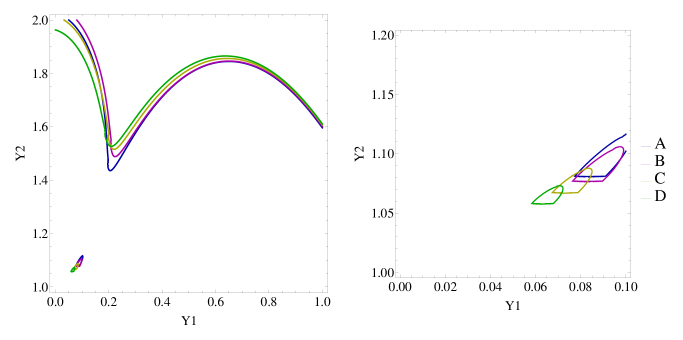
Figure 2: Plots of lines with the best fit value of $R=32$ in the parameter space of $(Y_{1},Y_{2})$. Left: The full range of the space examined. Right: A close plot of a small portion of the parameter space taken from the full plot. The curves have $(Y_{3},Z_{1},Z_{2})$ values set as follows: $A=(1.08,0.05,0.02)$, $B=(1.08,0.0,0.08)$, $C=(1.07,0.002,0.77)$, and $D=(1.06,0.01,0.065)$.

The fit depends on a total of six coefficients, as can be seen from examining the undiagonalised effective mass matrix. Optimising $R$, we should also attempt to find mixing angles in line with those known to parameterize the neutrino sector - i.e. large $\theta_{23}$ and $\theta_{12}$, with a comparatively small (but non-zero) $\theta_{13}$. This is necessary to obtain results compatible with neutrino oscillation experiments. Table 6 summarises the neutrino parameters the model must be in keeping with in order to be acceptable. We should note that the parameter $m_{0}$ will be trivially matched up with the mass differences shown in Table 6.

If we take some choice values of three of our five free parameters, we can construct a contour plot for curves with constant R using the other two. Figure 2 shows this for a series of fixed parameters. Each of the lines is for $R=32$, so we can see that there is a deal of flexibility in the parameter space for finding allowed values of the ratio.

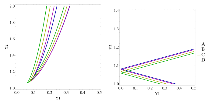
Figure 3: The figures show plots of two large neutrino mixing angles at their current best fit values. Left: Plot of $\sin^{2}(\theta_{12})=0.306$, Right: Plot of $\sin^{2}(\theta_{23})=0.446$. The curves have $(Y_{3},Z_{1},Z_{2})$ values set as follows: $A=(1.08,0.05,0.02)$, $B=(1.08,0.0,0.08)$, $C=(1.07,0.002,0.77)$, and $D=(1.06,0.01,0.065)$.

• In order to further determine which parts of the broad parameter space are most suitable for returning phenomenologically acceptable neutrino parameters, we can plot the value of $\sin^{2}(\theta_{12})$ or $\sin^{2}(\theta_{23})$ in the same parameter space as Figure 2 - $(Y_{1},Y_{2})$. The first plot in Figure 3 shows that the angle $\theta_{12}$ constraints are best satisfied at lower values of $Y_{1}$, while there are the each line spans a large part of the $Y_{2}$ space. The second plot of Figure 3 suggests a preference for comparatively small values of $Y_{2}$ based on the constraints on $\theta_{23}$. As such, we might expect that for this corner of the parameter space there will be some solutions that satisfy all the constraints.

Figure 4 also shows a plot for contours of best fitting values of $R$, with the free variables chosen as $Y_{3}$ and $Z_{1}$. As before, this shows that for a range of the other parameters, we can usually find suitable values of $(Y_{3},Z_{1})$ that satisfy the constraints on $R$. This being the case, we expect that it should be possible to find benchmark points that will allow for the other constraints to also be satisfied.

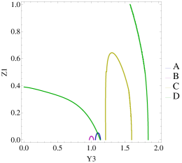
Figure 4: Plots of lines with the best fit value of $R=32$ in the parameter space of $(Y_{3},Z_{1})$. The curves have $(Y_{1},Y_{2},Z_{2})$ values set as follows: $A=(\frac{1}{5},1.4,0.02)$, $B=(0.05,1.5,0.01)$, $C=(\frac{1}{2},1.6,0.01)$, and $D=(\frac{2}{3},1.8,0.5)$.

This flexibility in the parameter space translates to the other experimental parameters, such that the points that allow experimentally allowed solutions are abundant enough that we can fit all the parameters quite well. Table 7 shows a collection of so-called benchmark points, which are points in the parameter space where all constraints are satisfied within current experimental errors - see Table 6. The table only shows values where $\theta_{23}$ is in the first octant. We might expect that the model should also admit solutions for second octant $\theta_{23}$, however attempts as numerical solution indicate this possibility is strongly disfavoured. We also note that current Planck data [57] puts the sum of neutrino masses to be $\Sigma m_{\nu}\leq 0.23\text{eV}$, which the bench mark points are also consistent with.

Inputs
$Y_{1}$	0.08	0.09	0.09	0.10
$Y_{2}$	1.09	1.10	1.10	1.11
$Y_{3}$	1.07	1.08	1.08	1.09
$Z_{1}$	0.01	0.01	0.00	0.01
$Z_{2}$	0.07	0.08	0.08	0.08
$m_{0}$	54.0meV	51.6meV	50.3meV	47.8meV
Outputs
$\theta_{12}$	33.5	33.2	33.1	32.8
$\theta_{13}$	8.70	8.82	9.05	9.05
$\theta_{23}$	41.9	41.7	41.7	41.5
$m_{1}$	53.4meV	51.1meV	49.8meV	47.3meV
$m_{2}$	54.1meV	51.8meV	50.5meV	48.1meV
$m_{3}$	73.2meV	71.5meV	70.8meV	69.1meV

Table 7: Table of Benchmark values in the Parameter space, where all experimental constraints are satisfied within errors. These point are samples of the space of all possible points, where we assume $\theta_{23}$ is in the first octant. All inputs are given to two decimal places, while the outputs are given to 3s.f.

3.9 Proton decay

Proton decay is a recurring problem in many $SU(5)$ GUT models, with the “dangerous” dimension six operators, with the effective operator form:

$$\ \frac{QQQL}{\Lambda^{2}}\,,\,\frac{d^{c}u^{c}u^{c}e^{c}}{\Lambda^{2}}\,,\,\frac{\bar{e}^{c}\bar{u}^{c}QQ}{\Lambda^{2}}\,,\,\frac{\bar{d}^{c}\bar{u}^{c}QL}{\Lambda^{2}}\,.$$ (42)

Since there are strong bounds on the proton lifetime ($\tau_{p}\geq 10^{3}3\text{yr}$) then these operators should be highly suppressed or not allowed in any GUT model.

Within the context of the $SU(5)\times A_{4}\times U(1)$ in F-theory, these operators arise from effective operators of the type:

$$10\cdot 10\cdot 10\cdot\bar{5}\,,$$ (43)

where the $\bar{5}$ contains the $SU(2)$ Lepton doublet and the $d^{c}$, and the quark doublet, $u^{c}$ and $e^{c}$ arise from $10$ of $SU(5)$. The interaction will be mediated by the $H_{u}$ and $H_{d}$ doublets.

In the model under consideration, two matter curves are in the $10$ representation of the GUT group: $T_{3}$ containing the third generation, and $T$ containing the lighter two generations. In general these can be expressed as:

$$\begin{gathered}T^{i}\cdot T^{j}_{3}\cdot F\\ i+j=3\,\,\text{and}\,\,i,j\in\{0,1,2,3\}\end{gathered}$$ (44)

Here, the role of R-symmetry in the model becomes important, since due to the assignment of this symmetry, these operators are all disallowed. Further more, the operators which have $i\neq 0$ will have net charge due to the $U(1)_{\perp}$, requiring them to have flavons to balance the charge. This would offer further suppression in the event that R-symmetry were not enforced.

There are also proton decay operators mediated by $D$-Higgs triplets and their anti-particles, which arise from the same operators, but in a similar way, these will be disallowed by R-symmetry thus preventing proton decay via dimension six operators.

The dimension four operators, which are mediated by superpartners of the Standard Model, will also be prevented by R-symmetry. However, even in the absence of this symmetry, the need to balance the charge of the $U(1)_{\perp}$ would lead to the presence of additional GUT group singlets in the operators, leading to further, strong suppression of the operator.

3.10 Unification

The spectrum in Table 4 is equivalent to three families of quarks and leptons plus three families of $5+\overline{5}$ representations which include the two Higgs doublets that get VEVs. Such a spectrum does not by itself lead to gauge coupling unification at the field theory level, and the splittings which may be present in F-theory cannot be sufficiently large to allow for unification, as discussed in [25]. However, as discussed in [25], where the low energy spectrum is identical to this model (although achieved in a different way) there may be additional bulk exotics which are capable of restoring gauge coupling unification and so unification is certainly possible in this mode. We refer the reader to the literature for a full discussion.

4 $S_{3}$ models

Motivated by phenomenological explorations of the neutrino properties under $S_{3}$, in this section we are interested for $SU(5)$ with $S_{3}$ discrete symmetry and its subgroup $Z_{3}$. More specifically, we analyse monodromies which induce the breaking of $SU(5)_{\perp}$ to group factors containing the aforementioned non-abelian discrete group. Indeed, in this section we encountered two such symmetry breaking chains, namely cases $ii$) and $iii)$ of (2). With respect to the present point of view, novel features are found for case $iii)$. In the subsequent we present in brief case $ii)$ and next we analyse in detail case $iii)$.

4.1 The ${\cal C}_{3}\times{\cal C}_{2}$ spectral cover split

As in the $A_{4}$ case, because these discrete groups originate form the $SU(5)_{\perp}$ we need to work out the conditions on the associated coefficients $a_{i}$. For ${\cal C}_{3}\times{\cal C}_{2}$ split the spectral cover equation is

$$P_{5}=\sum_{k}b_{k}s^{5-k}=P_{a}P_{b}=(a_{0}+a_{1}s+a_{2}s^{2}+a_{3}s^{3})\,(a_{4}+a_{5}s+a_{6}s^{2})$$ (45)

The equations connecting $b_{k}$’s with $a_{i}$’s are of the form $b_{k}\sim\sum_{n}a_{n}a_{9-n-k}$, the sum referring to appropriate values of $n$ which can be read off from (45) or from Table 1. We recall that the $b_{k}$ coefficients are characterised by homologies $[b_{k}]=\eta-k\,c_{1}$. Using this fact as well as the corresponding equations $b_{k}(a_{i})$ given in the last column of Table 1, we can determine the corresponding homologies of the $a_{i}$’s in terms of only one arbitrary parameter which we may take to be the homology $[a_{6}]=\chi$. Furthermore the constraint $b_{1}=a_{2}a_{6}+a_{3}a_{5}=0$ is solved by introducing a suitable section $\lambda$ such that $a_{3}=-\lambda\,a_{6}$ and $a_{2}=\lambda\,a_{5}$.

Apart from the constraint $b_{1}=0$, there are no other restrictions on the coefficients $a_{i}$ in the case of the $S_{3}$ symmetry. If, however, we wish to reduce the $S_{3}$ symmetry to $A_{3}$ (which from the point of view of low energy phenomenology is essentially $Z_{3}$), additional conditions should be imposed. In this case the model has an $SU(5)\times Z_{3}\times U(1)$ symmetry. As in the case of $A_{4}$ discussed previously, in order to derive the constraints on $a_{k}$’s for the symmetry reduction $S_{3}\to Z_{3}$ we compute the discriminant, which turns out to be

$$\Delta=\left(a_{1}^{2}-4a_{0}a_{2}\right)a_{2}^{2}-27a_{0}^{2}a_{3}^{2}+2a_{1}\left(9a_{0}a_{2}-2a_{1}^{2}\right)a_{3}\,,$$ (46)

and demand $\Delta=\delta^{2}$. In analogy with the method followed in $A_{4}$ we re-organise the terms in powers of the $x\equiv a_{1}$:

$$\Delta\to f(x)=-4a_{3}x^{3}+a_{2}^{2}x^{2}+18a_{0}a_{2}a_{3}x-a_{0}\left(4a_{2}^{3}+27a_{0}a_{3}^{2}\right)\,.$$ (47)

First, we observe that in order to write the above expression as a square, the product $a_{1}a_{3}$ must be positive definite ${\rm sign}(a_{1}a_{3})=+$. Provided this condition is fulfilled, then we require the vanishing of the discriminant $\Delta_{f}$ of the cubic polynomial $f(x)$, namely:

$$\Delta_{f}=-64a_{0}a_{3}\left(27a_{0}a_{3}^{2}-a_{2}^{3}\right){}^{3}=0\,.$$

This can occur if the non-trivial relation $a_{2}^{3}=27a_{0}a_{3}^{2}$ holds. Substituting back to (46) we find that the condition is fulfilled for $a_{2}^{2}\propto a_{1}a_{3}$. The two constraints can be combined to give the simpler ones

$$a_{0}a_{3}+a_{1}a_{2}=0,\;\;a_{2}^{2}+27a_{1}a_{3}=0$$

The details concerning the spectrum, homologies and flux restrictions of this model can be found in [19, 22]. Identifying $t_{1,2,3}=t_{a}$ and $t_{4,5}=t_{b}$ ( due to monodromies) we distribute the matter and Higgs fields over the curves as follows

$$10_{M}\equiv 10_{t_{b}},\;\bar{5}_{h_{d}}\equiv\bar{5}_{t_{a}+t_{b}},\;5_{h_{u}}\equiv 5_{-2t_{b}},\;\bar{5}_{2t_{a}}=\bar{5}_{M},$$

and the allowed tree-level couplings with non-trivial $SU(5)$ representations are

$$\begin{split}{\cal W}&=y_{u}\,10_{M}\,10_{M}\,\bar{5}_{h_{u}}+y_{d}\,10_{M}\,\bar{5}_{M}\,\bar{5}_{h_{d}}\end{split}$$ (48)

We have already pointed out that the monodromies organise the $SU(5)_{GUT}$ singlets $\theta_{ij}$ obtained from the $24\in SU(5)_{\perp}$ into two categories. One class carries $U(1)_{i}$-charges and they denoted with $\theta_{ab}$, $\theta_{ba}$ while the second class $\theta_{aa},\theta_{bb}$ has no $t_{i}$-‘charges’. The KK excitations of the latter could be identified with the right-handed neutrinos. Notice that in the present model the left handed states of the three families reside on the same matter curve. To generate flavour and in particular neutrino mixing in this model, one may appeal for example to the mechanism discussed in [44]. Detailed phenomenological implications for $Z_{3}$ models have been discussed elsewhere and will not be presented here. Within the present point of view, novel interesting features are found in $3+1+1$ splitting which will be discussed in the next sections.

4.2 $SU(5)$ spectrum for the $(3,1,1)$ factorisation

In this case the relevant spectral cover polynomial splits into three factors according to

$$\sum_{k=0}^{5}b_{k}s^{5-k}=\left(a_{4}s^{3}+a_{3}s^{2}+a_{2}s+a_{1}\right)\left(a_{5}+sa_{6}\right)\left(a_{7}+sa_{8}\right)$$

We can easily extract the equations determining the coefficients $b_{k}(a_{i})$, while the corresponding one for the homologies reads

$$[b_{k}]=\eta-kc_{1}=[a_{l}]+[a_{m}]+[a_{n}],\;k=0,1,\dots,5,\;k+l+m+n=18,\;l,m,n\leq 8$$ (49)

As in the previous case, in order to embed the symmetry in $SU(5)_{\perp}$, the condition $b_{1}=0$ has to be implemented.

The non-trivial representations are found as follows: The tenplets are determined by

$$b_{5}=a_{1}a_{5}a_{7}=0$$

As before, the equation for fiveplets is given by ${\cal R}=b_{3}^{2}b_{4}-b_{2}b_{3}b_{5}+b_{0}b_{5}^{2}=0$. Substitution of the relevant equations $b_{k}=b_{k}(a_{i})$ given in Table 1 and the condition $b_{1}=0$ result in the factorisation

$$\begin{split}{\cal R}&=\left(a_{1}a_{6}a_{8}+a_{2}\left(a_{6}a_{7}+a_{5}a_{8}\right)\right)\times\left(a_{1}a_{6}+a_{5}\left(a_{2}-ca_{5}a_{7}\right)\right)\\ &\times\left(a_{7}\left(a_{2}-ca_{5}a_{7}\right)+a_{1}a_{8}\right)\times\left(a_{6}a_{7}+a_{5}a_{8}\right)\end{split}$$ (50)

The four factors determine the homologies of the fiveplets dubbed $5_{a},5_{b},5_{c},5_{d}$ correspondingly. These, together with the tenplets, are given in Table 8.

Curve	equation	homology	$U(1)_{Y}$	$U(1)_{X}$
$10_{t_{i}}=10_{a}$	$a_{1}$	$\eta-3c_{1}-{\chi}-\psi$	$-N_{\chi}-N_{\psi}$	$M_{10_{a}}$
$10_{t_{4}}=10_{b}$	$a_{5}$	$-c_{1}+\chi$	$N_{\chi}$	$M_{10_{b}}$
$5_{-t_{i}-t_{j}}=5_{a}$	$a_{1}a_{6}a_{8}+a_{2}\left(a_{6}a_{7}+a_{5}a_{8}\right)$	$\eta-3c_{1}$	$0$	$M_{5_{a}}$
$5_{-t_{i}-t_{4}}=5_{b}$	$a_{1}a_{6}+a_{5}\left(a_{2}-ca_{5}a_{7}\right)$	$\eta-3c_{1}-{\psi}$	$-N_{\psi}$	$M_{5_{b}}$
$5_{-t_{i}-t_{5}}=5_{c}$	$a_{7}\left(a_{2}-ca_{5}a_{7}\right)+a_{1}a_{8}$	$\eta-3c_{1}-{\chi}$	$-N_{\chi}$	$M_{5_{c}}$
$5_{-t_{4}-t_{5}}=5_{d}$	$a_{6}a_{7}+a_{5}a_{8}$	$-c_{1}+{\chi}+\psi$	$N_{\chi}+N_{\psi}$	$M_{5_{d}}$
$10_{t_{5}}=10_{c}$	$a_{7}$	$-c_{1}+\psi$	$N_{\psi}$	$M_{10_{c}}$

Table 8: Matter curves with their defining equations, homologies, and multiplicities in the case of (3,1,1) factorisation.

4.3 ${\cal S}_{3}$ and ${\cal Z}_{3}$ models for $(3,1,1)$ factorisation

In the following we present one characteristic example of F-theory derived effective models when we quotient the theory with a ${\cal S}_{3}$ monodromy. As already stated, if no other conditions are imposed on $a_{k}$ this model is considered as an $S_{3}$ variant of the $3+1+1$ example given in [19, 22]. In this case the $10_{t_{i}},i=1,2,3$ residing on a curve - characterised by a common defining equation $a_{1}=0$ - are organised in two irreducible $S_{3}$ representations $2+1$. The same reasoning applies to the remaining representations. In Table 9 we present the spectrum of a model with $N_{\chi}=-1$ and $N_{\psi}=0$. Because singlets play a vital role, here, in addition we include the singlet field spectrum. Notice that the multiplicities of $\theta_{i4},\theta_{4i}$ are not determined by the $U(1)$ fluxes assumed here, hence they are treated as free parameters.

$\quad\quad{SU(5)\times{S_{3}}}$	$N_{Y}$-flux	$M_{X}$	Matter
$10_{a}^{(1)}=(10,1)_{M}$	$+1$	$1$	$Q+2e^{c}$
$10_{a}^{(2)}=(10,2)_{M}$	$0$	$1$	$2(Q+u^{c}+e^{c})$
$\overline{10}_{b}=(\overline{10},1)$	$-1$	$0$	$u^{c}+\bar{e}^{c}$
$5^{(1)}_{a}=(5,1)$	$0$	$1$	$h_{u}+D$
$5^{(2)}_{a}=(5,2)$	$0$	$1$	$2(h_{u}^{\prime}+D^{\prime})$
$\overline{5}^{(1)}_{b}=(\overline{5},1)_{M}$	$0$	$-1$	$\ell+d^{c}$
$\overline{5}^{(2)}_{b}=(\overline{5},2)_{M}$	$0$	$-1$	$2(\ell+d^{c})$
$\overline{5}^{(1)}_{c}=(\overline{5},1)$	$1$	$-1$	$\bar{D}$
$\overline{5}^{(2)}_{c}=(\overline{5},2)$	$0$	$-1$	$2(h_{d}^{\prime}+\bar{D}^{\prime})$
$\bar{5}_{d}=(\overline{5},1)$	$-1$	$0$	$h_{d}$
$10_{c}$	$0$	$0$	empty

Table 9: Matter content for an $SU(5)_{GUT}\times{S_{3}}\times{U(1)}$. $S_{3}$ monodromy organises $10_{a}$,$5_{a}$,$5_{b}$ and $5_{c}$ representations in doublets and singlets.

4.4 The Yukawa matrices in $S_{3}$ Models

To construct the mass matrices in the case of $S_{3}$ models we first recall a few useful properties. There are six elements of the group in three classes, and their irreducible representations are 1, $\textbf{1}^{\prime}$ and 2. The tensor product of two doublets, in the real representation, contains two singlets and a doublet:

$${\bf 2\otimes{2}}={\bf 1}\oplus{\bf{1}^{\prime}}\oplus{\bf 2}$$ (51)

Thus, if $(x_{1},x_{2})$ and $(y_{1},y_{2})$ represent the components of the doublets, the above product gives

$${\bf 1}:(x_{1}y_{1}+x_{2}y_{2}),\quad{{\bf{1}^{\prime}}:(x_{1}y_{2}-x_{2}y_{1})},\quad{{\bf 2}:\left(\begin{array}[]{l}x_{1}y_{2}+x_{2}y_{1}\\ x_{1}y_{1}-x_{2}y_{2}\end{array}\right)}.$$ (52)

The singlets are muliplied according to the rules: ${\bf 1}\otimes{{\bf 1}^{\prime}}=\bf{1}^{\prime}$ and ${\bf 1}^{\prime}\otimes{{\bf 1}^{\prime}}=\bf{1}$. Note that $\textbf{1}^{\prime}$ is not an $S_{3}$ invariant. With these simple rules in mind, we proceed with the construction of the fermion mass matrices, starting from the quark sector.

4.5 Quark sector

We start our analysis of the Top-type quarks. We see from table 9 that we have two types of operators contribute to the Top-type quark matrix.

1) A tree level coupling: $g10_{a}^{(2)}\cdot{10_{a}^{(2)}}\cdot{5_{a}^{(1)}}$

2) Dimension 4 operators: $\lambda_{1}10_{a}^{(1)}\cdot{10_{b}^{(1)}}\cdot{5_{a}^{(1)}}\cdot{\theta_{a}^{(1)}}$ and $\lambda_{2}10_{a}^{(2)}\cdot{10_{b}^{(1)}}\cdot{5_{a}^{(1)}}\cdot{\theta_{a}^{(2)}}$

In order to generate a hierarchical mass spectrum we accommodate the charm and top quarks in the $10_{a}^{(2)}$ curve and the first generation on the $10_{a}^{(1)}$ curve. In this case, only the first (tree level) coupling contributes to the Top quark terms. Using the $S_{3}$ algebra above while choosing $\langle{5_{a}^{1}}\rangle=\langle{H_{u}}\rangle=\upsilon_{u}$ and $\langle{\theta_{a}^{1}}\rangle=\theta_{0}$, $\langle{\theta_{a}^{2}}\rangle=(\theta_{1},0)^{\text{T}}$ we obtain the following mass matrix for the Top-quarks

$$m_{u}={\left(\begin{array}[]{ccc}\lambda_{1}\theta_{0}&\lambda_{2}\theta_{1}&0\\ 0&\epsilon g&0\\ 0&0&g\end{array}\right)\upsilon_{u}}$$ (53)

Because two generations live on the same matter curve ($10_{a}^{(2)}$ curve) we implement the Rank theorem. For this reason we have suppressed the element-22 in the matrix above with a small scale parameter $\epsilon$. The quark eigenmasses are obtained from $V_{u}^{L\dagger}m_{u}m_{u}^{\dagger}V_{u}^{L}=(m_{u}^{diag})^{2}$ where the transformation matrix $V_{u}^{L}$ is required for CKM-matrix along with the transformation of Bottom-type quark masses $V_{d}^{L}$ such that $V_{CKM}=V_{u}^{L\dagger}V_{d}^{L}$. By setting $x=\lambda_{1}\theta_{0}$, $y=\lambda_{2}\theta_{1}$ and $g=z$ we have

$$m_{u}m_{u}^{\dagger}={\left(\begin{array}[]{ccc}x^{2}+y^{2}&\epsilon yz&0\\ \epsilon yz&\epsilon^{2}z^{2}&0\\ 0&0&z^{2}\end{array}\right)\upsilon_{u}^{2}}$$ (54)

For reasonable values of the parameters this matrix leads to mass eigenvalues with the required mass hierarchy and a Cabbibo mixing angle. The smaller mixing angles are expected to be generated from the down quark mass matrix. Indeed, the following Yukawa couplings emerge for the Bottom-type quarks:

1) First generation: $g_{1}10_{a}^{(1)}\cdot{\bar{5}_{b}^{(1)}}\cdot{\bar{5}_{d}}\cdot{\theta_{a}^{(1)}}$.

2) Second and third generation: $g_{2}10_{a}^{(2)}\cdot{\bar{5}_{b}^{(2)}}\cdot{\bar{5}_{d}}\cdot{\theta_{a}^{(1)}}$.

3) First-second, third generation: $g_{3}10_{a}^{(2)}\cdot{\bar{5}_{b}^{(1)}}\cdot{\bar{5}_{d}}\cdot{\theta_{a}^{(2)}}$ and $g_{4}10_{a}^{(1)}\cdot{\bar{5}_{b}^{(2)}}\cdot{\bar{5}_{d}}\cdot{\theta_{a}^{(2)}}$.

4) Second-third generation: $g_{5}10_{a}^{(2)}\cdot{\bar{5}_{b}^{(2)}}\cdot{\bar{5}_{d}}\cdot{\theta_{a}^{(2)}}$.

We assume that the doublet $H_{d}\in{\bar{5}_{b}^{(1)}}$ and the singlet ${\theta_{a}^{2}}$ (being a doublet under $S_{3}$) develop VEVs designated as $\langle{H_{d}\rangle}=\upsilon_{d}$ and $\langle{\theta_{a}^{2}}\rangle=(\theta_{1},\theta_{2})^{\text{T}}$. Then, applying the $S_{3}$ algebra, the Yukawa couplings above induce the following mass matrix for the Bottom-type quarks:

$$m_{d}={\left(\begin{array}[]{ccc}g_{1}\theta_{0}&g_{3}\theta_{1}&g_{3}\theta_{2}\\ g_{4}\theta_{1}&g_{2}\theta_{0}+g_{5}\theta_{2}&g_{5}\theta_{1}\\ g_{4}\theta_{2}&g_{5}\theta_{1}&g_{2}\theta_{0}-g_{5}\theta_{2}\end{array}\right)\upsilon_{d}}.$$ (55)

For appropriate Singlet VEVs the structure of the Bottom quark mass matrix is capable to reproduce the hierarchical mass spectrum and the required CKM mixing.

4.6 Leptons

The charged leptons will have the same couplings as the Bottom-type quarks. To simplify the analysis, let us start with a simple case where the Singlet VEVs exhibit the hierarchy $\theta_{2}<\theta_{1}<\theta_{0}$. Furthermore, taking the limit $\theta_{2}\rightarrow{0}$ and switching-off the Yukawas coefficients $g_{3}$, $g_{4}$ in (55) we achieve a block diagonal form of the charged lepton matrix

$$m_{\ell}={\left(\begin{array}[]{ccc}g_{1}\theta_{0}&0&0\\ 0&g_{2}\theta_{0}&g_{5}\theta_{1}\\ 0&g_{5}\theta_{1}&g_{2}\theta_{0}\end{array}\right)\upsilon_{d}}.$$ (56)

with eigenvalues

$$\begin{split}m_{e}=g_{1}\theta_{0},\;m_{\mu}=g_{2}\theta_{0}-g_{5}\theta_{1},\;m_{\tau}=g_{2}\theta_{0}+g_{5}\theta_{1}\end{split}$$ (57)

and maximal mixing between the second and third generations.

We turn now our attention to the couplings of the neutrinos. We identify the right-handed neutrinos with the SU(5)-singlet $\theta_{c}=1_{ij}$. Under the $S_{3}$ symmetry, $\theta_{c}$ splits into a singlet, named $\theta_{c}^{(1)}$ and a doublet, $\theta_{c}^{(2)}$. As in the case of the quarks and the charged leptons we distribute the right handed neutrino species as follows

$$\theta_{c}^{(1)}\rightarrow{\nu_{1}^{c}}\quad\quad{\textrm{and}}\quad\quad\theta_{c}^{(2)}\rightarrow{(\nu_{2}^{c}\quad{\nu_{3}^{c}})^{\text{T}}}$$

The Dirac neutrino mass matrix arises from the following couplings

1) $y_{1}5_{a}^{(1)}\cdot{\bar{5}_{b}^{(1)}}\cdot{\theta_{c}^{(1)}}\cdot{\theta_{a}^{(1)}}$

2) $y_{2}5_{a}^{(1)}\cdot{\bar{5}_{b}^{(2)}}\cdot{\theta_{c}^{(2)}}\cdot{\theta_{a}^{(1)}}$

3) $y_{3}5_{a}^{(1)}\cdot{\bar{5}_{b}^{(2)}}\cdot{\theta_{c}^{(1)}}\cdot{\theta_{a}^{(2)}}$

4) $y_{4}5_{a}^{(1)}\cdot{\bar{5}_{b}^{(1)}}\cdot{\theta_{c}^{(2)}}\cdot{\theta_{a}^{(2)}}$

5) $y_{5}5_{a}^{(1)}\cdot{\bar{5}_{b}^{(2)}}\cdot{\theta_{c}^{(2)}}\cdot{\theta_{a}^{(2)}}$

and has the following form (for $\theta_{2}\rightarrow{0}$)

$${\cal M}_{D}={\left(\begin{array}[]{ccc}y_{1}\theta_{0}&y_{3}\theta_{1}&0\\ y_{4}\theta_{1}&y_{2}\theta_{0}&y_{5}\theta_{1}\\ 0&y_{5}\theta_{1}&y_{2}\theta_{0}\end{array}\right)\upsilon_{u}}$$ (58)

Although the Dirac mass matrix has the same form with the charged lepton matrix (55) in general they have different Yukawas coefficients. Thus, substantial mixing effects may also occur even in the case of a diagonal heavy Majorana mass matrix.

In the following we construct effective neutrino mass matrices compatible with the well known neutrino data in two different ways. In the first approach we take the simplest scenario for a diagonal heavy Majorana mass matrix and generate the TB-mixing combining charged lepton and neutrino block-diagonal textures. In the second case we consider the most general form of the Majorana matrix and we try to generate TB-mixing only from the Neutrino sector.

4.6.1 Block diagonal case

We start with the attempt to generate the TB-mixing combining charged lepton and neutrino block-diagonal textures. The Majorana matrix will simply be the identity matrix scaled by a RH-neutrino mass $M$. The effective neutrino mass matrix $M_{eff}=M_{D}M_{M}^{-1}M_{D}^{\text{T}}$ now reads:

$${\cal M}_{\nu}^{eff}=\left(\begin{array}[]{ccc}y_{1}^{2}\theta_{0}^{2}+y_{3}^{2}\theta_{1}^{2}&(y_{2}y_{3}+y_{1}y_{4})\theta_{0}\theta_{1}&y_{3}y_{5}\theta_{1}^{2}\\ (y_{2}y_{3}+y_{1}y_{4})\theta_{0}\theta_{1}&y_{2}^{2}\theta_{0}^{2}+(y_{4}^{2}+y_{5}^{2})\theta_{1}^{2}&2y_{2}y_{5}\theta_{0}\theta_{1}\\ y_{3}y_{5}\theta_{1}^{2}&2y_{2}y_{5}\theta_{0}\theta_{1}&y_{2}^{2}\theta_{0}^{2}\end{array}\right)\frac{\upsilon_{u}^{2}}{M}$$ (59)

where we used the Dirac mass matrix as given in (58). First of all we observe that we can reduce the number of the parameters by defining

$$\theta_{0}=\epsilon\theta_{1},\;x=y_{2}\epsilon,\;y=y_{1}\epsilon,\;a=y_{3},\;b=y_{4},\;c=y_{5}.$$

Then ${\cal M}_{\nu}^{eff}$ is written

$${\cal M}_{\nu}^{eff}=\left(\begin{array}[]{ccc}y^{2}+a^{2}&xa+yb&ac\\ xa+yb&x^{2}+b^{2}+c^{2}&2xc\\ ac&2xc&x^{2}\end{array}\right)\frac{\upsilon_{u}^{2}\theta_{1}^{2}}{M}$$ (60)

In the limit of a small $y_{5}$ Yukawa (or $c\rightarrow{0}$) we achieve a block diagonal form given by

$${\cal M}_{\nu}^{eff}=\left(\begin{array}[]{ccc}y^{2}+a^{2}&xa+yb&0\\ xa+yb&x^{2}+b^{2}&0\\ 0&0&x^{2}\end{array}\right)\frac{\upsilon_{u}^{2}\theta_{1}^{2}}{M}$$ (61)

This can be diagonalised by a unitary matrix

$$V_{\nu}=\left(\begin{array}[]{ccc}\cos(\theta_{12})&\sin(\theta_{12})&0\\ -\sin(\theta_{12})&\cos(\theta_{12})&0\\ 0&0&1\\ \end{array}\right)$$ (62)

Now, we may appeal to the block diagonal form of the charged lepton matrix (56) which introduces a maximal $\theta_{23}$ angle so that the final mixing is

$$U_{eff}=\left(\begin{array}[]{ccc}\cos(\theta_{12})&\sin(\theta_{12})&0\\ -\cos(\theta_{23})\sin(\theta_{12})&\cos(\theta_{12})\cos(\theta_{23})&\sin(\theta_{23})\\ \sin(\theta_{12})\sin(\theta_{23})&-\cos(\theta_{12})\sin(\theta_{23})&\cos(\theta_{23})\\ \end{array}\right)$$

Indeed, a quick calculation in the 2-3 block of charged lepton matrix (56) gives:

$$\cos{(2\theta_{23})}=0\rightarrow{\theta_{23}=\frac{\pi}{4}}$$

Moreover, diagonalisation of the neutrino mass matrix yields

$$\tan(2\theta_{12})=\frac{2(x\alpha+yb)}{y^{2}+\alpha^{2}-x^{2}-b^{2}}$$ (63)

The TB-mixing matrix now arises for $\tan{(2\theta_{12})}\approx{2.828}$. In figure (5) we plot contours for the above relation in the plane ($\alpha,x$) for various values of the pairs $(b,y)$.As can be observed, $\tan{(2\theta_{12})}$ takes the desired value for reasonable range of the parameters $\alpha,b,x,y$. For example

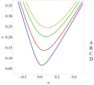
Figure 5: Curves for the relation $\tan{(2\theta_{12})}=2.828$ in the parameter space of $(\alpha,x)$ . The curves have (b,y) values set as follows: $A=(\frac{2}{5},\frac{4}{7})$, $B=(\frac{1}{3},\frac{1}{2})$, $C=(\frac{4}{13},\frac{1}{2})$ and $D=(\frac{2}{7},\frac{1}{2})$.

$$\tan{(2\theta_{12})}\approx{2.804}\quad\quad{for}\quad\quad(\alpha,b,x,y)=(\frac{2}{7},\frac{2}{9},\frac{1}{4},\frac{3}{8})$$ (64)

We conclude that the simplified (block-diagonal) forms of the charged lepton and neutrino mass matrices are compatible with the TB-mixing. It is easy now to obtain the known deviations of the TB-mixing allowing small values for the parameters $c,\theta_{2}$ in (56) and (61) respectively. However, we also need to reconcile the ratio of the mass square differences $R=\Delta m^{2}_{32}/\Delta m^{2}_{21}$ with the experimental data $R\approx 32$. To this end, we first compute the mass eigenvalues of the effective neutrino mass matrix

$$m_{1} =x^{2}$$

$$m_{2} =\frac{1}{2}(a^{2}+b^{2}+x^{2}+y^{2}-\Delta)$$

$$m_{3} =\frac{1}{2}(a^{2}+b^{2}+x^{2}+y^{2}+\Delta)$$

where $\Delta=\sqrt{[(\alpha+b)^{2}+(x-y)^{2}][(\alpha-b)^{2}+(x+y)^{2}]}$. Notice that $\Delta$ is a positive quantity and as a result $m_{3}>m_{2}$.

We can find easily solutions for a wide range of the parameters consistent with the experimental data. Note that for the same values as in (64) we achieve a reasonable value of $R\approx{28.16}$. In figure(6) we plot contours of the ratio in the plane ($\alpha$, $b$) for various values of the pair ($x,y$).

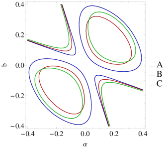
Figure 6: Contour plot for the ratio $R=\Delta m^{2}_{32}/\Delta m^{2}_{21}=32$ in the parameter space $(\alpha,b)$. The curves correspond to the following $(x,y)$ values: $A=(\frac{1}{4},\frac{3}{8})$, $B=(\frac{2}{7},\frac{1}{2})$, and $C=(\frac{2}{7},\frac{3}{7})$ .

We have stressed above that we could generate the $\theta_{13}$ angle by assuming small values of the Yukawas $y_{5}$. However, this case turns out to be too restrictive since the structure of (61) results to maximal $(1-2)$ mixing in contradiction with the experiment. The issue could be remedied by a fine-tuning of the charged lepton mixing, however we would like to look up for a natural solution. Therefore, we proceed with other options.

4.6.2 TB mixing from neutrino sector.

In the previous analysis we considered the simplest scenario for the Majorana matrix. The general form of the Majorana mass matrix arises by taking into account all the possible flavon terms contributions and has the following form

$$M_{maj}=\left(\begin{array}[]{lll}M&f_{1}&f_{2}\\ f_{1}&m&f_{3}\\ f_{2}&f_{3}&m\end{array}\right)$$ (65)

with $M>m>f_{i}$.

To reduce the number of parameters we consider that $f_{i}=f$ for $i=1,2,3$ and $y_{3},y_{4}\rightarrow{0}$ in the Dirac matrix. In this case the elements of the effective neutrino mass matrix are

$$\begin{split}M_{11}&=(a^{2}-b^{2})y^{2}\\ M_{12}&=M_{13}=M_{21}=M_{31}=bx(b-a)(y+c)\\ M_{22}&=M_{33}=(a-b^{2})x^{2}+(a+b^{2})c^{2}-2(b-1)bxc\\ M_{23}&=M_{32}=b(b-1)(x^{2}+c^{2})-2(b^{2}-a)xc\\ \end{split}$$ (66)

with an overall factor $\sim\frac{\upsilon_{u}^{2}\theta_{1}^{2}M^{2}}{(2f^{3}-2f^{2}m-f^{2}M+m^{2}M)}$ and the parameters are defined as $a=m/M$, $b=f/M$, $c=y_{5}$, $x=\epsilon y_{2}$, $y=\epsilon y_{1}$ and $\theta_{0}=\epsilon\theta_{1}$. The matrix assumes the general structure:

$$M_{\nu}=\left(\begin{array}[]{lll}p&q&q\\ q&r&s\\ q&s&r\end{array}\right)$$ (67)

Maximal atmospheric neutrino mixing and $\theta_{13}=0$ immediately follow from this structure. The solar mixing angle $\theta_{12}$ is not predicted, but it is expected to be large.

Next we try to generate TB -mixing only from the neutrino sector (assuming that the charged lepton mixing is negligible so that it can be used to lift $\theta_{13}\neq 0$). Then, it is enough to compare the entries of the effective mass matrix with the most general mass matrix form which complies with TB-mixing

$$m_{\nu}=\left(\begin{array}[]{lll}u&v&v\\ v&u+w&v-w\\ v&v-w&u+w\end{array}\right)$$ (68)

A quick comparison results to the following simple relations

$$\begin{split}u&=M_{11}\\ v&=M_{12}\\ w&=M_{22}-u=M_{22}-M_{11}\\ \end{split}$$ (69)

while the (23) element is subject to the constraint:

$$v=M_{23}+w$$ (70)

which results to a quadratic equation of $b$ with solutions being functions of the remaining parameters $b=B_{\pm}(a,c,x,y)$. We choose one of the roots, $b=B_{-}$, and substitute it back to the equations (69) to express the parameters $u$, $v$ and $w$ as functions of $(a,c,x,y)$.

The requirement that all the large mixing effects emerge from the neutrino sector imposes severe restrictions on the parameter space. Hence we need to check their compatibility with the mass square differences ratio $R$. We can express the latter as a function of the parameters $R=R(a,c,x,y)$ by noting that the mass eigenvalues are given by

$$m_{1}=u-v,\quad{m_{2}=u+2v},\quad{m_{3}=u-v+2w}$$

Direct substitution gives the desired expression $R(a,c,x,y)$ which is plotted in figure 7. It is straightforward to notice that there is a wide range of parameters consistent with the experimental data. In the first graph of the figure we plot contours for the ratio in the plane $(x,y)$ for various values of $a$ and constant value $c=0.5$. In the second graph we plot the ratio in the $(a,c)$ plane with constant $x=0.33$. Note that in both cases, the $a,c,x,y$ parameters take values $<1$.

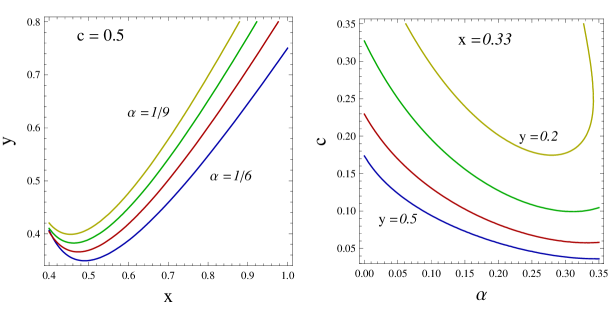
Figure 7: Contour plots for the ratio $R=\Delta m^{2}_{32}/\Delta m^{2}_{21}=32$ in the parameter spaces $(x,y)$-left and $(a,c)$-right. In the first plot (left) $c=0.5$ and $a_{blue}=\frac{1}{6}$, $a_{red}=\frac{1}{7}$, $a_{green}=\frac{1}{8}$ and $a_{yellow}=\frac{1}{9}$. In the $(a,c)$ plot $x=0.33$ and $a_{blue}=0.5$, $a_{red}=0.4$, $a_{green}=0.3$ and $a_{yellow}=0.2$.

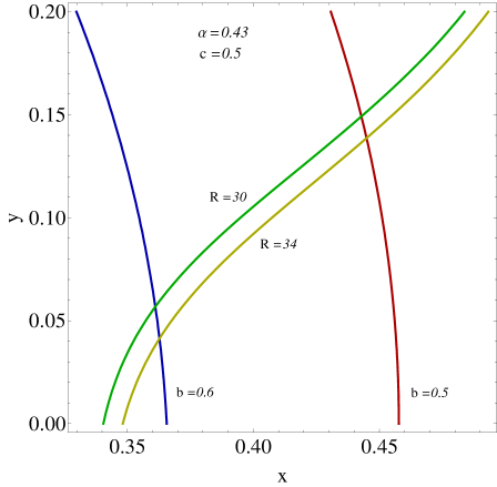
Figure 8: Bounds in the parameter space $(x,y)$ from the experimental data and the requirement $b<1$.

Having checked that the parameters $a,c,x,y$ are in the perturbative range, while consistent with the TB-mixing and the mass data, we also should require that $b=f/M$ remains in the perturbative regime, i.e. $b<1$. In figure 8 we plot the bounds put by this constraint. In particular we plot the mass square ratio in the $(x,y)$ plane for $R=30$ and $R=34$ and we notice that there exists an overlapping region for values of $b$ between 0.5 and 0.6. In this region $x\sim{0.4}$ and $y\sim{0.1}$. More precisely a typical set of such values gives

$$(a,c,x,y)=(\frac{3}{7},\frac{1}{2},\frac{2}{5},\frac{1}{10})\rightarrow{b\approx{0.5}}\quad\textrm{and}\quad{R\approx{31.5}}.$$

5 Conclusions

In this work we considered the phenomenological implications of F-theory $SU(5)$ models with non-abelian discrete family symmetries. We discussed the physics of these constructions in the context of the spectral cover, which, in the elliptical fibration and under the specific choice of $SU(5)$ GUT, implies that the discrete family symmetry must be a subgroup of the permutation symmetry $S_{5}$. Furthermore, we exploited the topological properties of the associated 5-degree polynomial coefficients (inherited from the internal manifold) to derive constraints on the effective field theory models. Since we dealt with discrete gauge groups, we also proposed a discrete version of the flux mechanism for the splitting of representations. We started our analysis splitting appropriately with the spectral cover in order to implement the $A_{4}$ discrete symmetry as a subgroup of $S_{4}$. Hence, using Galois Theory techniques, we studied the necessary conditions on the discriminant in order to reduce the symmetry from $S_{4}$ to $A_{4}$. Moreover, we derived the properties of the matter curves accommodating the massless spectrum and the constraints on the Yukawa sector of the effective models. Then, we first made a choice of our flux parameters and picked up a suitable combination of trivial and non-trivial $A_{4}$ representations to accommodate the three generations so that a hierarchical mass spectrum for the charged fermion sector is guaranteed. Next, we focused on the implications of the neutrino sector. Because of the rich structure of the effective theory emerging from the covering $E_{8}$ group, we found a considerable number of Yukawa operators contributing to the neutrino mass matrices. Despite their complexity, it is remarkable that the F-theory constraints and the induced discrete symmetry organise them in a systematic manner so that they accommodate naturally the observed large mixing effects and the smaller $\theta_{13}$ angle of the neutrino mixing matrix.

In the second part of the present article, using the appropriate factorisation of the spectral cover we derive the $S_{3}$ group as a family symmetry which accompanies the $SU(5)$ GUT. Because now the family symmetry is smaller than before, the resulting fermion mass structures turn out to be less constrained. In this respect, the $A_{4}$ symmetry appears to be more predictive. Nevertheless, to start with, we choose to focus on a particular region of the parameter space assuming some of the Yukawa matrix elements are zero and imposing a diagonal heavy Majorana mass matrix. In such cases, we can easily derive block diagonal lepton mass matrices which incorporate large neutrino mixing effects as required by the experimental data. Next, in a more involved example, we allow for a general Majorana mass matrix and initially determine stable regions of the parameter space which are consistent with TB-mixing. The tiny $\theta_{13}$ angle can easily arise from small deviations of these values or by charged lepton mixing effects. Both models derived here satisfy the neutrino mass squared difference ratio predicted by neutrino oscillation experiments.

In conclusion, F-theory $SU(5)$ models with non-abelian discrete family symmetries provide a promising theoretical framework within which the flavour problem may be addressed. The present paper presents the first such realistic examples based on $A_{4}$ and $S_{3}$, which are amongst the most popular discrete symmetries used in the field theory literature in order to account for neutrino masses and mixing angles. By formulating such models in the framework of F-theory $SU(5)$, a deeper understanding of the origin of these discrete symmetries is obtained, and theoretical issues such as doublet-triplet splitting may be elegantly addressed.

Acknowledgements

The research of AK and GKL has been co-financed by the European Union (European Social Fund - ESF) and Greek national funds through the Operational Program ”Education and Lifelong Learning” of the National Strategic Reference Framework (NSRF) - Research Funding Program: ”THALIS”. Investing in the society of knowledge through the European Social Fund. SFK acknowledges the EU ITN grant INVISIBLES 289442. AKM is supported by an STFC studentship.

Appendix A Block Diagonalisation of $A_{4}$

A.1 Four dimensional case

From considering the symmetry properties of a regular tetrahedron, we can see quite easily that it can be parameterised by four coordinates and its transformations can be decomposed into a mere two generators. If we write these coordinates as a basis for $A_{4}$, which is the symmetry group of the tetrahedron, it would be of the form $\left(t_{1},t_{2},t_{3},t_{4}\right)^{\text{T}}$. The two generators can then be written in matrix form explicitly as:

$$S=\left(\begin{array}[]{cccc}0&0&0&1\\ 0&0&1&0\\ 0&1&0&0\\ 1&0&0&0\end{array}\right)\,\,\,\text{and}\,\,\,T=\left(\begin{array}[]{cccc}1&0&0&0\\ 0&0&0&1\\ 0&1&0&0\\ 0&0&1&0\end{array}\right)\,\,.$$ (71)

However, it is well known that $A_{4}$ has an irreducible representation in the form of a singlet and triplet under these generators. If we consider the tetrahedron again, this can be physically interpreted by observing that under any rotation through one of the vertices of the tetrahedron the vertex chosen remains unmoved under the transformation. In order to find the irreducible representation, we must note some conditions that this decomposition will satisfy.

In order to obtain the correct basis, we must find a unitary transformation $V$ that block diagonalises the generators of the group. As such, we have the following conditions:

$$\begin{gathered}VSV^{\text{T}}=S^{\prime}=\left(\begin{array}[]{cccc}1&0&0&0\\ 0&-&-&-\\ 0&-&-&-\\ 0&-&-&-\end{array}\right)\,,\\ VTV^{\text{T}}=T^{\prime}=\left(\begin{array}[]{cccc}1&0&0&0\\ 0&-&-&-\\ 0&-&-&-\\ 0&-&-&-\end{array}\right)\,,\\ VV^{\text{T}}=\text{I}_{4x4}\,\,,\end{gathered}$$ (72)

as well as the usual conditions that must be satisfied by the generators: $S^{2}=T^{3}=(ST)^{3}=\text{I}$. It will also be useful to observe three extra conditions, which will expedite finding the solution. Namely that the block diagonal of one of the two generators must have zeros on the diagonal to insure the triplet changes within itself.

If we write an explicit form for V,

$$V=\left(\begin{array}[]{cccc}v_{11}&v_{12}&v_{13}&v_{14}\\ v_{21}&v_{22}&v_{23}&v_{24}\\ v_{31}&v_{32}&v_{33}&v_{34}\\ v_{41}&v_{42}&v_{43}&v_{44}\end{array}\right)\,,$$ (73)

we can extract a set of quadratic equations and attempt to solve for the elements of the matrix. Note that we have assumed as a starting point that $v_{ij}\in\mathbb{R}\forall i,j$. The complete list is included in the appendix. The problem is quite simple, but at the same time would be awkward to solve numerically, so we shall attempt to simplify the problem analytically first. If we start be using:

$$\begin{gathered}v_{11}^{2}+v_{12}^{2}+v_{13}^{2}+v_{14}^{2}=1\,,\\ \text{\&}\,\,\,2v_{12}v_{13}+2v_{11}v_{14}=1\,,\end{gathered}$$ (74)

we can trivially see two quadratics,

$$(v_{11}-v_{14})^{2}+(v_{12}-v_{13})^{2}=0\,.$$ (75)

Since we assume that all our elements or V are real numbers, it must be true then that:

$$v_{11}=v_{14}\,\,\,\text{and}\,\,\,v_{12}=v_{13}\,.$$ (76)

We may now substitute this result into a number of equations. However, we chose to focus on the following two:

$$\begin{gathered}v_{11}v_{21}+v_{12}v_{23}+v_{13}v_{24}+v_{14}v_{22}\rightarrow v_{11}(v_{21}+v_{22})+v_{12}(v_{23}+v_{24})\,\,\,\text{and}\\ v_{11}v_{21}+v_{12}v_{24}+v_{13}v_{22}+v_{14}v_{23}\rightarrow v_{11}(v_{21}+v_{23})+v_{12}(v_{22}+v_{24})\,.\end{gathered}$$ (77)

Taking the difference of these two equations, we can easily see there is a solution where $v_{11}=v_{12}$, and as such by the previous result:

$$v_{11}=v_{12}=v_{13}=v_{14}=\pm\frac{1}{2}\,.$$ (78)

We are free to choose whichever sign for these four elements we please, provided they all have the same sign. This outcome reduces the number of useful equations to twelve, as nine of them can be summarised as

$$\sum_{i}v_{2i}=\sum_{i}v_{3i}=\sum_{i}v_{4i}=0\,.$$ (79)

Let us consider the first of these three derived conditions, along with the conditions:

$$\begin{gathered}v_{21}^{2}+v_{22}^{2}+v_{23}^{2}+v_{24}^{2}=1\,,\\ v_{21}^{2}+v_{22}v_{23}+v_{22}v_{24}+v_{23}v_{24}=0\,.\end{gathered}$$ (80)

Squaring the condition $\sum_{i}v_{2i}=0$ and using these relations, we can derive easily that $v_{21}=\pm\frac{1}{2}$. Likewise we can derive the same for $v_{31}$ and $v_{41}$. As before, we might chose either sign for each of these elements, with each possibility yielding a different outcome for the basis, though our choices will constrain the signs of the remaining elements in V.

Let us make a choice for the signs of our known coefficients in the matrix and choose them all to be positive for simplicity. We are now left with a much smaller set of conditions:

$$\begin{gathered}\sum_{i=2}^{4}v_{ji}=-\frac{1}{2}\,\,,\\ \sum_{i=2}^{4}v_{ji}^{2}=\frac{3}{4}\,\,\,\text{and}\\ \sum_{i=2}^{4}v_{ji}v_{ki}=\frac{1}{4}\,\,,\\ j,k\in\{2,3,4\}\,\,\,\text{and}\,\,\,k\neq j\,\,\,.\end{gathered}$$ (81)

After a few choice rearrangements, these coefficients can be calculated numerically in Mathematica. This yields a unitary matrix,

$$V=\frac{1}{2}\left(\begin{array}[]{cccc}1&1&1&1\\ 1&-1&-1&1\\ 1&-1&1&-1\\ 1&1&-1&-1\end{array}\right)\,,$$ (82)

up to exchanges of the bottom three rows, which arises due to the fact the triplet arising in this representation may be ordered arbitrarily. There is also a degree of choice involved regarding the sign of the rows. However, this is again largely unimportant as the result would be equivalent.

If we apply this transformation to our original basis $t_{i}$, we find that we have a singlet and a triplet in the new basis,

$$\begin{gathered}t_{singlet}=t_{1}+t_{2}+t_{3}+t_{4}\\ t_{triplet}=\left(t_{1}-t_{2}-t_{3}+t_{4},\,t_{1}-t_{2}+t_{3}-t_{4}\,,t_{1}+t_{2}-t_{3}-t_{4}\right)\,,\end{gathered}$$ (83)

and that our generators become block-diagonal:

$$\begin{gathered}S^{\prime}=\left(\begin{array}[]{cccc}1&0&0&0\\ 0&1&0&0\\ 0&0&-1&0\\ 0&0&0&-1\end{array}\right)\\ T^{\prime}=\left(\begin{array}[]{cccc}1&0&0&0\\ 0&0&1&0\\ 0&0&0&1\\ 0&1&0&0\end{array}\right)\,.\end{gathered}$$ (84)

A.1.1 List of Conditions

$$\begin{gathered}0)\,\,\,v_{ij}\in\mathbb{R}\forall i,j\\ \text{1-4})\,\,\,\sum_{j=1}^{4}v_{ij}^{2}=1\,\,\,i\in\left\{1,2,3,4\right\}\\ 5)\,\,\,v_{11}v_{21}+v_{12}v_{22}+v_{13}v_{23}+v_{14}v_{24}=0\\ 6)\,\,\,v_{11}v_{31}+v_{12}v_{32}+v_{13}v_{33}+v_{14}v_{34}=\\ 7)\,\,\,v_{11}v_{41}+v_{12}v_{42}+v_{13}v_{43}+v_{14}v_{44}=0\\ 8)\,\,\,v_{21}v_{31}+v_{22}v_{32}+v_{23}v_{33}+v_{24}v_{34}=0\\ 9)\,\,\,v_{21}v_{41}+v_{22}v_{42}+v_{23}v_{43}+v_{24}v_{44}=0\\ 10)\,\,\,v_{31}v_{41}+v_{32}v_{42}+v_{33}v_{43}+v_{34}v_{44}=0\\ 11)\,\,\,2v_{12}v_{13}+2v_{11}v_{14}=1\\ 12)\,\,\,v_{11}v_{24}+v_{12}v_{23}+v_{13}v_{22}+v_{14}v_{21}=0\\ 13)\,\,\,v_{11}v_{34}+v_{12}v_{33}+v_{13}v_{32}+v_{14}v_{31}=0\\ 14)\,\,\,v_{11}v_{44}+v_{12}v_{43}+v_{13}v_{42}+v_{14}v_{41}=0\\ 15)\,\,\,v_{11}^{2}+v_{12}v_{13}+v_{12}v_{14}+v_{13}v_{14}=1\\ 16)\,\,\,v_{11}v_{21}+v_{12}v_{24}+v_{13}v_{22}+v_{14}v_{23}=0\\ 17)\,\,\,v_{11}v_{31}+v_{12}v_{34}+v_{13}v_{32}+v_{14}v_{33}=0\\ 18)\,\,\,v_{11}v_{41}+v_{12}v_{44}+v_{13}v_{42}+v_{14}v_{43}=0\\ 19)\,\,\,v_{11}v_{21}+v_{12}v_{23}+v_{13}v_{24}+v_{14}v_{22}=0\\ 20)\,\,\,v_{11}v_{31}+v_{12}v_{33}+v_{13}v_{34}+v_{14}v_{32}=0\\ 21)\,\,\,v_{11}v_{41}+v_{12}v_{43}+v_{13}v_{44}+v_{14}v_{42}=0\\ 22)\,\,\,v_{21}^{2}+v_{22}v_{23}+v_{22}v_{24}+v_{23}v_{24}=0\\ 23)\,\,\,v_{31}^{2}+v_{32}v_{33}+v_{32}v_{34}+v_{33}v_{34}=0\\ 24)\,\,\,v_{41}^{2}+v_{42}v_{43}+v_{42}v_{44}+v_{43}v_{44}=0\\ \end{gathered}$$ (85)

Appendix B Yukawa coupling algebra

Table 5 specifies all the allowed operators for the $N=0$ $SU(5)\times A_{4}\times U(1)$ model discussed in the main text. Here we include the full algebra for calculation of the Yukawa matrices given in the text. All couplings must have zero $t_{5}$ charge, respect R-symmetry and be $A_{4}$ singlets. In the basis derived in Appendix A, we have the triplet product:

$$\begin{gathered}3_{a}\times 3_{b}=1+1^{\prime}+1^{\prime\prime}+3_{1}+3_{2}\\ 1=a_{1}b_{2}+a_{2}b_{2}+a_{3}b_{3}\\ 1^{\prime}=a_{1}b_{2}+\omega a_{2}b_{2}+\omega^{2}a_{3}b_{3}\\ 1^{\prime\prime}=a_{1}b_{2}+\omega^{2}a_{2}b_{2}+\omega a_{3}b_{3}\\ 3_{1}=(a_{2}b_{3},\,a_{3}b_{1},\,a_{1}b_{2})^{\text{T}}\\ 3_{2}=(a_{3}b_{2},\,a_{1}b_{3},\,a_{2}b_{1})^{\text{T}}\end{gathered}$$

where $3_{a}=(a_{1},\,a_{2},\,a_{3})^{\text{T}}$ and $3_{b}=(b_{1},\,b_{2},\,b_{3})^{\text{T}}$.

B.1 Top-type quarks

The top-type quarks have four non-vanishing couplings, while the $T\cdot T_{3}\cdot H_{u}\cdot\theta_{a}\cdot\theta_{a}$ and $T\cdot T\cdot H_{u}\cdot\theta_{a}\cdot\theta_{a}\cdot\theta_{b}$ couplings vanishings due to the chosen vacuum expectations: $\langle H_{u}\rangle=(v,0,0)^{\text{T}}$ and $\langle\theta_{a}\rangle=(a,0,0)^{\text{T}}$.

The contribution to the heaviest generation self-interaction is due to the $T_{3}\cdot T_{3}\cdot H_{u}\cdot\theta_{a}$ operator:

$$(1\times 1)\times(3\times 3) \rightarrow 1\times 1$$

$$\rightarrow 1$$

$$(T_{3}\times T_{3})\times H_{u}\times\theta_{a} \rightarrow(T_{3}\times T_{3})va$$

We note that this is the lowest order operator in the top-type quarks, so should dominate the hierarchy.

The interaction between the third generation and the lighter two generations is determined by the $T\cdot T_{3}\cdot H_{u}\cdot\theta_{a}\cdot\theta_{b}$ operator:

$$(1\times 1)\times(3\times 3)\times 1 \rightarrow 1\times 1\times 1$$

$$\rightarrow 1$$

$$T\times T_{3}\times H_{u}\times\theta_{a}\times\theta_{b} \rightarrow vab$$

The remaining, first-second generation operators give contributions, in brief:

$$T\times T\times H_{u}\times\theta_{a}\times(\theta_{b})^{2} \rightarrow vab^{2}$$

$$T\times T\times H_{u}\times(\theta_{a})^{3} \rightarrow va^{3}$$

These will be subject to Rank Theorem arguments, so that only one of the generations directly gets a mass from the Yukawa interaction. However the remaining generation will gain a mass due to instantons and non-commutative fluxes, as in [37][38].

B.2 Charged Leptons

The charged Leptons and Bottom-type quarks come from the same operators in the GUT group, though in this exposition we shall work in terms of the Charged Leptons. The complication for Charged leptons is that the Left-handed doublet is an $A_{4}$ triplet, while the right-handed singlets of the weak interaction are singlets of the monodromy group. There are a total of six contributions to the Yukawa matrix, with the third generation right-handed types being generated by two operators.

The operators giving mass to the interactions of the right-handed third generation are dominated by the tree level operator $F\cdot H_{d}\cdot T_{3}$, which gives a contribution as:

$$3\times 3\times 1 \rightarrow 1\times 1\rightarrow 1$$

$$F\times H_{d}\times T_{3} \rightarrow y_{1}\left(\begin{array}[]{ccc}0&0&v_{1}\\ 0&0&v_{2}\\ 0&0&v_{3}\end{array}\right)$$

Clearly this should dominated the next order operator, however when we choose a vacuum expectation for the $H_{d}$ field, we will have contributions from $F\cdot H_{d}\cdot T_{3}\cdot\theta_{d}$:

$$3\times 3\times 3\times 1 \rightarrow 3\times 3\times 1\rightarrow 1$$

$$F\times H_{d}\times\theta_{d}\times T_{3} \rightarrow\left(\begin{array}[]{ccc}0&0&y_{2}v_{2}d_{3}+y_{3}v_{3}d_{2}\\ 0&0&y_{2}v_{3}d_{1}+y_{3}v_{1}d_{3}\\ 0&0&y_{2}v_{1}d_{2}+y_{3}v_{2}d_{1}\end{array}\right)$$

The generation of Yukawas for the lighter two generations comes, at leading order, from the operators $F\cdot H_{d}\cdot T\cdot\theta_{b}$ and $F\cdot H_{d}\cdot T\cdot\theta_{a}$:

$$F\times H_{d}\times T\times\theta_{b} \rightarrow y_{4}b\left(\begin{array}[]{ccc}v_{1}&v_{1}&0\\ v_{2}&v_{2}&0\\ v_{3}&v_{3}&0\end{array}\right)$$

$$F\times H_{d}\times T\times\theta_{a} \rightarrow y_{5}a\left(\begin{array}[]{ccc}0&0&0\\ v_{3}&v_{3}&0\\ v_{2}&v_{2}&0\end{array}\right)\,,$$

where the vacuum expectations for $\theta_{a}$ and $\theta_{b}$ are as before. The next order of operator take the same form, but with corrections due to the flavon triplet, $\theta_{d}$.

$$F\times H_{d}\times T\times\theta_{b}\times\theta_{d} \rightarrow\left(\begin{array}[]{ccc}y_{6}v_{2}d_{3}+y_{7}v_{3}d_{2}&y_{6}v_{2}d_{3}+y_{7}v_{3}d_{2}&0\\ y_{6}v_{3}d_{1}+y_{7}v_{1}d_{3}&y_{6}v_{3}d_{1}+y_{7}v_{1}d_{3}&0\\ y_{6}v_{1}d_{2}+y_{7}v_{2}d_{1}&y_{6}v_{1}d_{2}+y_{7}v_{2}d_{1}&0\end{array}\right)$$

$$F\times H_{d}\times T\times\theta_{a}\times\theta_{d} \rightarrow a\left(\begin{array}[]{ccc}y_{8}v_{1}d_{1}+y_{10}v_{2}d_{2}+y_{11}v_{3}d_{3}&y_{8}v_{1}d_{1}+y_{10}v_{2}d_{2}+y_{11}v_{3}d_{3}&0\\ y_{12}v_{1}d_{2}&y_{12}v_{1}d_{2}&0\\ y_{9}v_{1}d_{3}&y_{9}v_{1}d_{3}&0\end{array}\right)$$

B.3 Neutrinos

The neutrino sector admits masses of both Dirac and Majorana types. In the $A_{4}$ model, the right-handed neutrino is assigned to a matter curve constituting a singlet of the GUT group. However it is a triplet of the $A_{4}$ family symmetry, which along with the $SU(2)$ doublet will generate complicated structures under the group algebra.

B.3.1 Dirac Mass Terms

The Dirac mass terms coupling left and right-handed neutrinos comes from a maximum of four operators. The leading order operators are $\theta_{c}\cdot F\cdot H_{u}\cdot\theta_{b}$ and $\theta_{c}\cdot F\cdot H_{u}\cdot\theta_{a}$, where as we have already seen the GUT singlet flavons $\theta_{a}$ and $\theta_{b}$ are used to cancel $t_{5}$ charges. The right-handed neutrino is presumed to live on the GUT singlet $\theta_{d}$ .

The first of the operators, $\theta_{c}\cdot F\cdot H_{u}\cdot\theta_{b}$, contributes via two channels:

$$3\times 3\times 3\times 1 \rightarrow 3\times 3_{a}\times 1\rightarrow 1\times 1$$

$$\rightarrow\left(\begin{array}[]{c}c_{1}\\ c_{2}\\ c_{3}\end{array}\right)\times\left(\begin{array}[]{c}F_{2}v_{3}\\ F_{3}v_{1}\\ F_{1}v_{2}\end{array}\right)\times b\rightarrow y_{8}b\left(\begin{array}[]{ccc}0&0&v_{2}\\ v_{3}&0&0\\ 0&v_{1}&0\end{array}\right)$$

$$3\times 3\times 3\times 1 \rightarrow 3\times 3_{b}\times 1\rightarrow 1\times 1$$

$$\rightarrow\left(\begin{array}[]{c}c_{1}\\ c_{2}\\ c_{3}\end{array}\right)\times\left(\begin{array}[]{c}F_{3}v_{2}\\ F_{1}v_{3}\\ F_{2}v_{1}\end{array}\right)\times b\rightarrow y_{9}b\left(\begin{array}[]{ccc}0&v_{3}&0\\ 0&0&v_{1}\\ v_{2}&0&0\end{array}\right)$$

With the VEV alignments $$\langle\theta_{a}\rangle=(a,0,0)^{\text{T}} \langle H_{u}\rangle=(v,0,0)^{\text{T}}$$ and , we have a total matrix for the operator:

$$\rightarrow\left(\begin{array}[]{ccc}0&0&0\\ 0&0&y_{9}bv\\ 0&y_{8}bv&0\end{array}\right)$$

The second leading order operator, $\theta_{c}\cdot F\cdot H_{u}\cdot\theta_{a}$, is more cimplicated due to the presence of four $A_{4}$ triplet fields. The simpelst contribution to the operator is:

$$(3\times 3)\times(3\times 3) \rightarrow 1\times 1$$

$$\rightarrow\left(\begin{array}[]{ccc}y_{1}(v_{1}a_{1}+v_{2}a_{2}+v_{3}a_{3})&0&0\\ 0&y_{1}(v_{1}a_{1}+v_{2}a_{2}+v_{3}a_{3})&0\\ 0&0&y_{1}(v_{1}a_{1}+v_{2}a_{2}+v_{3}a_{3})\end{array}\right)\,,$$

which only contributes to the diagonal. This is accompanied by two similar operators in the way of:

$$(3\times 3)\times(3\times 3) \rightarrow 1^{\prime}\times 1^{\prime\prime}$$

$$\rightarrow(c_{1}F_{1}+\omega c_{2}F_{2}+\omega^{2}c_{3}F_{3})\times(v_{1}a_{1}+\omega^{2}v_{2}a_{2}+\omega v_{3}a_{3})$$

$$\rightarrow y_{2}\left(\begin{array}[]{ccc}v_{1}a_{1}&0&0\\ 0&v_{2}a_{2}&0\\ 0&0&v_{3}a_{3}\end{array}\right)$$

$$(3\times 3)\times(3\times 3) \rightarrow 1^{\prime\prime}\times 1^{\prime}$$

$$\rightarrow(c_{1}F_{1}+\omega^{2}c_{2}F_{2}+\omega c_{3}F_{3})\times(v_{1}a_{1}+\omega v_{2}a_{2}+\omega^{2}v_{3}a_{3})$$

$$\rightarrow y_{3}\left(\begin{array}[]{ccc}v_{1}a_{1}&0&0\\ 0&v_{2}a_{2}&0\\ 0&0&v_{3}a_{3}\end{array}\right)\,.$$

The remaining contribtuions are the complicated four-triplet products. However, upon retaining to our previous vacuum expectation values, these will all vanish, leaving an overall matrix of:

$$\rightarrow\left(\begin{array}[]{ccc}y_{0}va&0&0\\ 0&y_{1}va&0\\ 0&0&y_{1}va\end{array}\right)$$

Where $y_{0}=y_{1}+y_{2}+y_{3}$ as before. These contributions will produce a large mixing between the second and third generations, however they do not allow for mixing with the first generation.

Corrections from the next order operators will give a weaker mixing with the first generation. These correcting terms are $\theta_{c}\cdot F\cdot H_{u}\cdot\theta_{d}\cdot\theta_{b}$ and $\theta_{c}\cdot F\cdot H_{u}\cdot\theta_{d}\cdot\theta_{a}$, though we choose to only consider the first of these two operators, since the flavon $\theta_{a}$ will generate a very complicated structure, hindering computations with little obvious benefit in terms of model building. The $\theta_{c}\cdot F\cdot H_{u}\cdot\theta_{d}\cdot\theta_{b}$ operator has of diagonal contributions as:

$$(3\times 3)\times(3\times 3)\times 1 \rightarrow 3_{a}\times 3_{x}\times 1\rightarrow 1$$

$$\theta_{c}\times F\times H_{u}\times\theta_{d}\times\theta_{b} \rightarrow\left(\begin{array}[]{c}c_{2}F_{3}\\ c_{3}F_{1}\\ c_{1}F_{2}\end{array}\right)\times\left(\begin{array}[]{c}0\\ 0\\ vd_{2}\end{array}\right)\times b$$

$$\rightarrow\left(\begin{array}[]{ccc}0&0&0\\ z_{1}vd_{2}b&0&0\\ 0&0&0\end{array}\right)\,.$$

This is mirrored by similar combinations from the other 3 triplet-triplet combinations allowed by the algebra. Overall, this gives:

$$\rightarrow\left(\begin{array}[]{ccc}0&z_{3}vd_{2}b&z_{2}vd_{3}b\\ z_{1}vd_{2}b&0&0\\ z_{4}vd_{3}b&0&0\end{array}\right)\,.$$

Due to the choice of Higgs vacuum expectation, the diagonal contributions will only correct the first generation mass, giving a contribution to it $\sim vd_{1}b$.

B.3.2 Majorana operators

The right-handed neutrinos are also given a mass by Majorana terms. These are as it transpires relatively simple. The leading order term $\theta_{c}\cdot\theta_{c}$, gives a diagonal contribtuion:

$$3\times 3 \rightarrow 1$$

$$\theta_{c}\cdot\theta_{c} \rightarrow M\text{I}_{3\times 3}$$

There may also be corrections to the off diagonal, due to operators such as $\theta_{c}\cdot\theta_{c}\cdot\theta_{d}$. These yield:

$$3\times 3\times 3 \rightarrow 3\times 3\rightarrow 1$$

$$\theta_{c}\times\theta_{c}\times\theta_{d} \rightarrow\left(\begin{array}[]{ccc}0&d_{3}&d_{2}\\ d_{3}&0&d_{1}\\ d_{2}&d_{1}&0\end{array}\right)\,,$$

Higher orders of the flavon $\theta_{d}$ are also permitted, but should be suppressed by the coupling.

Appendix C Flux mechanism

For completeness, we discribe here in a simple manner the flux mechanism introduced to break symmetries and generate chirality.

$\bullet$ We start with the $U(1)_{Y}$-flux inside of $SU(5)_{GUT}$.

The ${\bf 5}$’s and ${\bf 10}$’s reside on matter curves $\Sigma_{5_{i}},\Sigma_{10_{j}}$ while are characterised by their defining equations. From the latter, we can deduce the corresponding homologies $\chi_{i}$ following the standard procedure. If we turn on a $U(1)_{Y}$-flux ${\cal F}_{Y}$, we can determine the flux restrictions on them which are expressed in terms of integers through the “dot product”

$$N_{Y_{i}}={\cal F}_{Y}\cdot\chi_{i}$$

The flux is responsible for the $SU(5)$ breaking down to the Standard Model and this can happen in such a way that the $U(1)_{Y}$ gauge boson remains massless [3, 2]. On the other hand, flux affects the multiplicities of the SM-representations carrying non-zero $U(1)_{Y}$-charge.

Thus, on a certain $\Sigma_{5_{i}}$ matter curve for example, we have

$${\bf 5}\in SU(5)\Rightarrow\left\{\begin{array}[]{lll}n_{(3,1)_{-\frac{1}{3}}}-n_{(\bar{3},1)_{\frac{1}{3}}}&=&{M_{5}}\\ n_{(1,2)_{\frac{1}{2}}}-n_{(1,2)_{-\frac{1}{2}}}&=&{M_{5}}+N_{Y_{i}}\end{array}\right.$$ (88)

where $N_{Y_{i}}={\cal F}_{Y}\cdot\chi_{i}$ as above. We can arrange for example $M_{5}+N_{Y_{i}}=0$ to eliminate the doublets or $M_{5}=0$ to eliminate the triplet.

$\bullet$ Let’s turn now to the $SU(5)\times S_{3}$. The $S_{3}$ factor is associated to the three roots $t_{1,2,3}$ which can split to a singlet and a doublet

$${\bf 1}_{S_{3}}=t_{s}=t_{1}+t_{2}+t_{3},\;{\bf 2}_{S_{3}}=\{t_{1}-t_{2},\;t_{1}+t_{2}-2t_{3}\}^{T}$$

It is convenient to introduce the two new linear combinations

$$t_{a}=t_{1}-t_{3},\;t_{b}=t_{2}-t_{3}$$

and rewrite the doublet as follows

$${\bf 2}_{S_{3}}=\left(\begin{array}[]{l}t_{a}-t_{b}\\ t_{a}+t_{b}\end{array}\right)\;\to\;\left(\begin{array}[]{l}-t_{b}\\ +t_{b}\end{array}\right)_{t_{a}}$$ (89)

Under the whole symmetry the $SU(5)_{GUT}$ ${\bf 10}_{t_{i}},i=1,2,3$ representations transform

$$({\bf 10},{\bf 1}_{S_{3}})+({\bf 10},{\bf 2}_{S_{3}})$$

Our intention is to turn on fluxes along certain directions. We can think of the following two different choices:

1) We can turn on a flux $N_{a}$ along $t_{a}$. The singlet $({\bf 10},{\bf 1}_{S_{3}})$ does not transform under $t_{a}$, hence this flux will split the multiplicities as follows

$${\bf 10}_{t_{i}}\Rightarrow\left\{\begin{array}[]{lll}({\bf 10},{\bf 1}_{S_{3}})&=&{M}\\ ({\bf 10},{\bf 2}_{S_{3}})&=&{M}+N_{a}\end{array}\right.$$ (92)

This choice will also break the $S_{3}$ symmetry to $Z_{3}$.

2) Turning on a flux along the singlet direction $t_{s}$ will preserve $S_{3}$ symmetry. The multiplicities now read

$${\bf 10}_{t_{i}}\Rightarrow\left\{\begin{array}[]{lll}({\bf 10},{\bf 1}_{S_{3}})&=&{M}+N_{s}\\ ({\bf 10},{\bf 2}_{S_{3}})&=&{M}\end{array}\right.$$ (95)

To get rid of the doublets we choose $M=0$ while because flux restricts non-trivially on the matter curve, the number of singlets can differ by just choosing $N_{s}\neq 0$.

Appendix D The $b_{1}=0$ constraint

To solve the $b_{1}=0$ constraint we have repeatidly introduced a new section $a_{0}$ and assumed factorisation of the involved $a_{i}$ coefficients. To check the validity of this assumption, we take as an example the $S_{3}\times Z_{2}$ case, where $b_{1}=a_{2}a_{6}+a_{3}a_{5}=0$. We note first that the coefficients $b_{k}$ are holomorphic functions of $z$, and as such they can be expressed as power series of the form $b_{k}=b_{k,0}+b_{k,1}z+\cdots$ where $b_{k,m}$ do not depend on $z$. Hence, the coefficients $a_{k}$ have a $z$-independent part

$$a_{k}=\sum_{m=0}a_{k,m}z^{m}$$

while the product of two of them can be cast to the form

$$a_{l}\,a_{k}=\sum_{p=0}\beta_{p}\,z^{p},\;\;{\rm with}\;\;\beta_{p}=\sum_{n=0}^{p}a_{ln}a_{k,p-n}$$

Clearly the condition $b_{1}=a_{2}a_{6}+a_{3}a_{5}=0$ has to be satisfied term-by-term. To this end, at the next to zeroth order we define

$$\lambda=\frac{a_{3,1}a_{5,0}+a_{2,1}a_{6,0}}{a_{5,1}a_{6,0}-a_{5,0}a_{6,1}}$$ (96)

The requirement $a_{5,1}a_{6,0}\neq a_{5,0}a_{6,1}$ ensures finiteness of $\lambda$, while at the same time excludes a relation of the form $a_{5}\propto\kappa a_{6}$ where $\kappa$ would be a new section.

We can write the expansions for $a_{2},a_{3}$ as follows

$$\ \begin{split}a_{2}&=\lambda a_{5,0}+a_{2,1}z+{\cal O}(z^{2})\\ a_{3}&=-\lambda a_{6,0}+a_{3,1}z+{\cal O}(z^{2})\end{split}$$ (97)

The $b_{1}=0$ condition is now

$$b_{1}=0+0\,z+{\cal O}(z^{2})$$

i.e., satified up to second order in $z$. Hence, locally we can set $z=0$ and simply write

$$a_{2}=\lambda\,a_{5},\;a_{3}=-\lambda\,a_{6}$$

References

- [1] C. Vafa, Nucl. Phys. B 469 (1996) 403 [arXiv:hep-th/9602022].
- [2] R. Donagi and M. Wijnholt, “Model Building with F-Theory,” Adv. Theor. Math. Phys. 15 (2011) 1237 [arXiv:0802.2969 [hep-th]].
- [3] C. Beasley, J. J. Heckman and C. Vafa, “GUTs and Exceptional Branes in F-theory - I,” JHEP 0901 (2009) 058 [arXiv:0802.3391 [hep-th]].
- [4] C. Beasley, J. J. Heckman and C. Vafa, JHEP 0901 (2009) 059 [arXiv:0806.0102 [hep-th]].
- [5] R. Blumenhagen, T. W. Grimm, B. Jurke and T. Weigand, Nucl. Phys. B 829 (2010) 325 [arXiv:0908.1784].
- [6] J. J. Heckman and C. Vafa, Nucl. Phys. B 837 (2010) 137 [arXiv:0811.2417 [hep-th]].
- [7] J. J. Heckman, J. Marsano, N. Saulina, S. Schafer-Nameki and C. Vafa, arXiv:0808.1286 [hep-th].
- [8] R. Blumenhagen, V. Braun, T. W. Grimm and T. Weigand, Nucl. Phys. B 815 (2009) 1 [arXiv:0811.2936 [hep-th]].
- [9] F. Denef, arXiv:0803.1194.
- [10] T. Weigand, Class. Quant. Grav. 27 (2010) 214004 [arXiv:1009.3497 [hep-th]].
- [11] J. J. Heckman, Ann. Rev. Nucl. Part. Sci. 60 (2010) 237 [arXiv:1001.0577 [hep-th]].
- [12] T. W. Grimm, Nucl. Phys. B 845 (2011) 48 [arXiv:1008.4133 [hep-th]].
- [13] G. K. Leontaris, PoS CORFU 2011 (2011) 095 [arXiv:1203.6277 [hep-th]].
- [14] A. Maharana and E. Palti, Int. J. Mod. Phys. A 28 (2013) 1330005 [arXiv:1212.0555 [hep-th]].
- [15] J. J. Heckman, A. Tavanfar and C. Vafa, JHEP 1008 (2010) 040 [arXiv:0906.0581 [hep-th]].
- [16] R. Donagi and M. Wijnholt, Adv. Theor. Math. Phys. 15 (2011) 1523 [arXiv:0808.2223 [hep-th]].
- [17] J. Marsano, N. Saulina and S. Schafer-Nameki, “Monodromies, Fluxes, and Compact Three-Generation F-theory GUTs,” JHEP 0908 (2009) 046 [arXiv:0906.4672 [hep-th]].
- [18] H. Hayashi, T. Kawano, Y. Tsuchiya and T. Watari, “Flavor Structure in F-theory Compactifications,” JHEP 1008 (2010) 036 [arXiv:0910.2762 [hep-th]].
- [19] E. Dudas and E. Palti, “On hypercharge flux and exotics in F-theory GUTs,” JHEP 1009 (2010) 013 [arXiv:1007.1297 [hep-ph]].
- [20] S. F. King, G. K. Leontaris and G. G. Ross, “Family symmetries in F-theory GUTs,” Nucl. Phys. B 838 (2010) 119 [arXiv:1005.1025 [hep-ph]].
- [21] J. C. Callaghan, S. F. King, G. K. Leontaris and G. G. Ross, “Towards a Realistic F-theory GUT,” JHEP 1204 (2012) 094 [arXiv:1109.1399 [hep-ph]].
- [22] I. Antoniadis and G. K. Leontaris, “Building SO(10) models from F-theory,” JHEP 1208 (2012) 001 [arXiv:1205.6930 [hep-th]].
- [23] J. C. Callaghan and S. F. King, “E6 Models from F-theory,” JHEP 1304 (2013) 034 [arXiv:1210.6913 [hep-ph]].
- [24] R. Tatar and W. Walters, “GUT theories from Calabi-Yau 4-folds with SO(10) Singularities,” JHEP 1212 (2012) 092 [arXiv:1206.5090 [hep-th]].
- [25] J. C. Callaghan, S. F. King and G. K. Leontaris, JHEP 1312 (2013) 037 [arXiv:1307.4593 [hep-ph]].
- [26] L. E. Ibanez and G. G. Ross, “Discrete gauge symmetry anomalies,” Phys. Lett. B 260 (1991) 291.
- [27] P. Anastasopoulos, M. Cvetic, R. Richter and P. K. S. Vaudrevange, “String Constraints on Discrete Symmetries in MSSM Type II Quivers,” JHEP 1303 (2013) 011 [arXiv:1211.1017 [hep-th]].
- [28] H. M. Lee, S. Raby, M. Ratz, G. G. Ross, R. Schieren, K. Schmidt-Hoberg and P. K. S. Vaudrevange, “A unique symmetry for the MSSM,” Phys. Lett. B 694 (2011) 491 [arXiv:1009.0905 [hep-ph]].
- [29] L. E. Ibanez, A. N. Schellekens and A. M. Uranga, “Discrete Gauge Symmetries in Discrete MSSM-like Orientifolds,” Nucl. Phys. B 865 (2012) 509 [arXiv:1205.5364 [hep-th]].
- [30] G. Honecker and W. Staessens, “To Tilt or Not To Tilt: Discrete Gauge Symmetries in Global Intersecting D-Brane Models,” JHEP 1310 (2013) 146 [arXiv:1303.4415 [hep-th]].
- [31] M. Berasaluce-Gonzalez, P. G. Camara, F. Marchesano, D. Regalado and A. M. Uranga, “Non-Abelian discrete gauge symmetries in 4d string models,” JHEP 1209 (2012) 059 [arXiv:1206.2383 [hep-th]].
- [32] G. Altarelli and F. Feruglio, “Discrete Flavor Symmetries and Models of Neutrino Mixing,” Rev. Mod. Phys. 82 (2010) 2701 [arXiv:1002.0211 [hep-ph]].
- [33] S. F. King and C. Luhn, “Neutrino Mass and Mixing with Discrete Symmetry,” Rept. Prog. Phys. 76 (2013) 056201 [arXiv:1301.1340 [hep-ph]].
- [34] S. F. King, A. Merle, S. Morisi, Y. Shimizu and M. Tanimoto, New J. Phys. 16 (2014) 045018 [arXiv:1402.4271 [hep-ph]].
- [35] I. Antoniadis and G. K. Leontaris, “Neutrino mass textures from F-theory,” Eur. Phys. J. C 73 (2013) 2670 [arXiv:1308.1581 [hep-th]].
- [36] R. Donagi and M. Wijnholt, Commun. Math. Phys. 326 (2014) 287 [arXiv:0904.1218 [hep-th]].
- [37] S. Cecotti, M. C. N. Cheng, J. J. Heckman and C. Vafa, arXiv:0910.0477 [hep-th].
- [38] L. Aparicio, A. Font, L. E. Ibanez and F. Marchesano, JHEP 1108 (2011) 152 [arXiv:1104.2609 [hep-th]].
- [39] F. Marchesano and L. Martucci, Phys. Rev. Lett. 104 (2010) 231601 [arXiv:0910.5496 [hep-th]].
- [40] A. Font, F. Marchesano, D. Regalado and G. Zoccarato, JHEP 1311 (2013) 125 [arXiv:1307.8089 [hep-th]].
- [41] C. Mayrhofer, E. Palti and T. Weigand, JHEP 1309 (2013) 082 [arXiv:1303.3589 [hep-th]].
- [42] S. F. King, Rept. Prog. Phys. 67 (2004) 107 [hep-ph/0310204].
- [43] N. Nakayama, “On Weierstrass models”, Algebraic Geometry and Commutative Algebra, Kinokuniya, Tokyo 1988
- [44] V. Bouchard, J. J. Heckman, J. Seo and C. Vafa, JHEP 1001 (2010) 061 [arXiv:0904.1419 [hep-ph]].
- [45] M. C. Gonzalez-Garcia, M. Maltoni, J. Salvado and T. Schwetz, JHEP 1212 (2012) 123 [arXiv:1209.3023 [hep-ph]].
- [46] J. Lesgourgues and S. Pastor, Adv. High Energy Phys. 2012 (2012) 608515 [arXiv:1212.6154 [hep-ph]].
- [47] D. C. Latimer and D. J. Ernst, Phys. Rev. D 71 (2005) 017301 [nucl-th/0405073].
- [48] P. Huber, Phys. Rev. C 84 (2011) 024617 [Erratum-ibid. C 85 (2012) 029901] [arXiv:1106.0687 [hep-ph]].
- [49] G. K. Leontaris and G. G. Ross, JHEP 1102 (2011) 108 [arXiv:1009.6000 [hep-th]].
- [50] C. Mayrhofer, E. Palti and T. Weigand, “U(1) symmetries in F-theory GUTs with multiple sections,” JHEP 1303 (2013) 098 [arXiv:1211.6742 [hep-th]].
- [51] J. Borchmann, C. Mayrhofer, E. Palti and T. Weigand, Phys. Rev. D 88 (2013) 046005 [arXiv:1303.5054 [hep-th]].
- [52] V. Braun, T. W. Grimm and J. Keitel, JHEP 1312 (2013) 069 [arXiv:1306.0577 [hep-th]].
- [53] M. Cvetic, D. Klevers and H. Piragua, JHEP 1306 (2013) 067 [arXiv:1303.6970 [hep-th]].
- [54] M. Cvetic, D. Klevers, H. Piragua and P. Song, arXiv:1310.0463 [hep-th].
- [55] J. Marsano, Phys. Rev. Lett. 106 (2011) 081601 [arXiv:1011.2212 [hep-th]].
- [56] S. Krippendorf, D. K. M. Pena, P. -K. Oehlmann and F. Ruehle, arXiv:1401.5084 [hep-th].
- [57] P. A. R. Ade et al. [Planck Collaboration], arXiv:1303.5076 [astro-ph.CO].
- [58] A. Font, L. E. Ibanez, F. Marchesano and D. Regalado, JHEP 1303 (2013) 140 [Erratum-ibid. 1307 (2013) 036] [arXiv:1211.6529 [hep-th]].