Reliable ABC model choice via random forests

Abstract

Approximate Bayesian computation (ABC) methods provide an elaborate approach to Bayesian inference on complex models, including model choice. Both theoretical arguments and simulation experiments indicate, however, that model posterior probabilities may be poorly evaluated by standard ABC techniques.

We propose a novel approach based on a machine learning tool named random forests to conduct selection among the highly complex models covered by ABC algorithms. We thus modify the way Bayesian model selection is both understood and operated, in that we rephrase the inferential goal as a classification problem, first predicting the model that best fits the data with random forests and postponing the approximation of the posterior probability of the predicted MAP for a second stage also relying on random forests. Compared with earlier implementations of ABC model choice, the ABC random forest approach offers several potential improvements: (i) it often has a larger discriminative power among the competing models, (ii) it is more robust against the number and choice of statistics summarizing the data, (iii) the computing effort is drastically reduced (with a gain in computation efficiency of at least fifty), and (iv) it includes an approximation of the posterior probability of the selected model. The call to random forests will undoubtedly extend the range of size of datasets and complexity of models that ABC can handle. We illustrate the power of this novel methodology by analyzing controlled experiments as well as genuine population genetics datasets.

The proposed methodologies are implemented in the R package abcrf available on the CRAN.

Keywords: Approximate Bayesian Computation, model selection, summary statistics, $k$-nearest neighbors, likelihood-free methods, random forests

1 Introduction

Approximate Bayesian Computation (ABC) represents an elaborate statistical approach to model-based inference in a Bayesian setting in which model likelihoods are difficult to calculate (due to the complexity of the models considered). Since its introduction in population genetics (Tavaré et al.,, 1997; Pritchard et al.,, 1999; Beaumont et al.,, 2002), the method has found an ever increasing range of applications covering diverse types of complex models in various scientific fields (see, e.g., Beaumont,, 2008; Toni et al.,, 2009; Beaumont,, 2010; Csillèry et al.,, 2010; Theunert et al.,, 2012; Chan et al.,, 2014; Arenas et al.,, 2015). The principle of ABC is to conduct Bayesian inference on a dataset through comparisons with numerous simulated datasets. However, it suffers from two major difficulties. First, to ensure reliability of the method, the number of simulations is large; hence, it proves difficult to apply ABC for large datasets (e.g., in population genomics where tens to hundred thousand markers are commonly genotyped). Second, calibration has always been a critical step in ABC implementation (Marin et al.,, 2012; Blum et al.,, 2013). More specifically, the major feature in this calibration process involves selecting a vector of summary statistics that quantifies the difference between the observed data and the simulated data. The construction of this vector is therefore paramount and examples abound about poor performances of ABC model choice algorithms related with specific choices of those statistics (Didelot et al.,, 2011; Robert et al.,, 2011; Marin et al.,, 2014), even though there also are instances of successful implementations.

We advocate a drastic modification in the way ABC model selection is conducted: we propose both to step away from selecting the most probable model from estimated posterior probabilities, and to reconsider the very problem of constructing efficient summary statistics. First, given an arbitrary pool of available statistics, we now completely bypass selecting among those. This new perspective directly proceeds from machine learning methodology. Second, we postpone the approximation of model posterior probabilities to a second stage, as we deem the standard numerical ABC approximations of such probabilities fundamentally untrustworthy. We instead advocate selecting the posterior most probable model by constructing a (machine learning) classifier from simulations from the prior predictive distribution (or other distributions in more advanced versions of ABC), known as the ABC reference table. The statistical technique of random forests (RF) (Breiman,, 2001) represents a trustworthy machine learning tool well adapted to complex settings as is typical for ABC treatments. Once the classifier is constructed and applied to the actual data, an approximation of the posterior probability of the resulting model can be produced through a secondary random forest that regresses the selection error over the available summary statistics. We show here how RF improves upon existing classification methods in significantly reducing both the classification error and the computational expense. After presenting theoretical arguments, we illustrate the power of the ABC-RF methodology by analyzing controlled experiments as well as genuine population genetics datasets.

2 Materials and methods

Bayesian model choice (Berger,, 1985; Robert,, 2001) compares the fit of $M$ models to an observed dataset $\mathbf{x}^{0}$. It relies on a hierarchical modelling, setting first prior probabilities $\pi(m)$ on model indices $m\in\{1,\ldots,M\}$ and then prior distributions $\pi(\theta|m)$ on the parameter $\theta$ of each model, characterized by a likelihood function $f(\mathbf{x}|m,\theta)$. Inferences and decisions are based on the posterior probabilities of each model $\pi(m|\mathbf{x}^{0})$.

2.1 ABC algorithms for model choice

While we cannot cover in much details the principles of Approximate Bayesian computation (ABC), let us recall here that ABC was introduced in Tavaré et al., (1997) and Pritchard et al., (1999) for solving intractable likelihood issues in population genetics. The reader is referred to, e.g., Beaumont, (2008), Toni et al., (2009), Beaumont, (2010), Csillèry et al., (2010) and Marin et al., (2012) for thorough reviews on this approximation method. The fundamental principle at work in ABC is that the value of the intractable likelihood function $f(\mathbf{x}^{0}|\theta)$ at the observed data $\mathbf{x}^{0}$ and for a current parameter $\theta$ can be evaluated by the proximity between $\mathbf{x}^{0}$ and pseudo-data $\mathbf{x}(\theta)$ simulated from $f(\mathbf{x}|\theta)$. In discrete settings, the indicator $\mathbb{I}(\mathbf{x}(\theta)=\mathbf{x}^{0})$ is an unbiased estimator of $f(\mathbf{x}^{0}|\theta)$ (Rubin,, 1984). For realistic settings, the equality constraint is replaced with a tolerance region $\mathbb{I}(d(\mathbf{x}(\theta),\mathbf{x}^{0})\leq\epsilon)$, where $d(\mathbf{x}^{0},\mathbf{x})$ is a measure of divergence between the two vectors and $\epsilon>0$ is a tolerance value. The implementation of this principle is straightforward: the ABC algorithm produces a large number of pairs $(\theta,\mathbf{x})$ from the prior predictive, a collection called the reference table, and extracts from the table the pairs $(\theta,\mathbf{x})$ for which $d(\mathbf{x}(\theta),\mathbf{x}^{0})\leq\epsilon$.

To approximate posterior probabilities of competing models, ABC methods (Grelaud et al.,, 2009) compare observed data with a massive collection of pseudo-data, generated from the prior predictive distribution in the most standard versions of ABC; the comparison proceeds via a normalized Euclidean distance on a vector of statistics $S(\mathbf{x})$ computed for both observed and simulated data. Standard ABC estimates posterior probabilities $\pi(m|\mathbf{x}^{0})$ at stage (B) of Algorithm 1 below as the frequencies of those models within the $k$ nearest-to-$\mathbf{x}^{0}$ simulations, proximity being defined by the distance between $S(\mathbf{x}^{0})$ and the simulated $S(\mathbf{x})$’s.

Selecting a model means choosing the model with the highest frequency in the sample of size $k$ produced by ABC, such frequencies being approximations to posterior probabilities of models. We stress that this solution means resorting to a $k$-nearest neighbor ($k$-nn) estimate of those probabilities, for a set of simulations drawn at stage (A), whose records constitute the so-called reference table, see Biau et al., (2015) or Stoehr et al., (2014).

Algorithm 1 ABC model choice algorithm

• Generate a reference table including $N_{\text{ref}}$ simulations $(m,S(\mathbf{x}))$ from $\pi(m)\pi(\theta|m)f(\mathbf{x}|m,\theta)$

• Learn from this set to infer about $m$ at $\mathbf{s}^{0}=S(\mathbf{x}^{0})$

Selecting a set of summary statistics $S(x)$ that are informative for model choice is an important issue. The ABC approximation to the posterior probabilities $\pi(m|\mathbf{x}^{0})$ will eventually produce a right ordering of the fit of competing models to the observed data and thus select the right model for a specific class of statistics on large datasets (Marin et al.,, 2014). This most recent theoretical ABC model choice results indeed show that some statistics produce nonsensical decisions and that there exist sufficient conditions for statistics to produce consistent model prediction, albeit at the cost of an information loss due to summaries that may be substantial. The toy example comparing MA(1) and MA(2) models in Appendix and Figure 1 clearly exhibits this potential loss in using only the first two autocorrelations as summary statistics. Barnes et al., (2012) developed an interesting methodology to select the summary statistics, but with the requirement to aggregate estimation and model pseudo-sufficient statistics for every model under comparison. That induces a deeply inefficient dimension inflation and can be very time consuming.

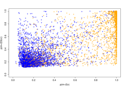
Figure 1: Illustration of the discrepancy between posterior probabilities based on the whole data and based on a summary. The aim is to choose between two nested time series models, namely moving averages of order 1 and 2 (denoted MA(1) and MA(2) respectively; see Appendix for more details). Each point of the plot gives two posterior probabilities of MA(2) for a dataset simulated either from the MA(1) (blue) or MA(2) model (orange), based on the whole data ($x$-axis) and on only the first two autocorrelations ($y$-axis).

It may seem tempting to collect the largest possible number of summary statistics to capture more information from the data. This brings $\pi(m|S(\mathbf{x}^{0}))$ closer to $\pi(m|\mathbf{x}^{0})$ but increases the dimension of $S(\mathbf{x})$. ABC algorithms, like $k$-nn and other local methods suffer from the curse of dimensionality (see e.g. Section 2.5 in Hastie et al., (2009)) so that the estimate of $\pi(m|S(\mathbf{x}^{0}))$ based on the simulations is poor when the dimension of $S(\mathbf{x})$ is too large. Selecting summary statistics correctly and sparsely is therefore paramount, as shown by the literature in the recent years. (See Blum et al., (2013) surveying ABC parameter estimation.) For ABC model choice, two main projection techniques have been considered so far. First, Prangle et al., (2014) show that the Bayes factor itself is an acceptable summary (of dimension one) when comparing two models, but its practical evaluation via a pilot ABC simulation induces a poor approximation of model evidences (Didelot et al.,, 2011; Robert et al.,, 2011). The recourse to a regression layer like linear discriminant analysis (LDA, Estoup et al.,, 2012) is discussed below and in Appendix Section A. Other projection techniques have been proposed in the context of parameter estimation: see, e.g., Fearnhead and Prangle, (2012); Aeschbacher et al., (2012).

Given the fundamental difficulty in producing reliable tools for model choice based on summary statistics (Robert et al.,, 2011), we now propose to switch to a different approach based on an adapted classification method. We recall in the next Section the most important features of the Random Forest (RF) algorithm.

2.2 Random Forest methodology

The Classification And Regression Trees (CART) algorithm at the core of the RF scheme produces a binary tree that sets allocation rules for entries as labels of the internal nodes and classification or predictions of $Y$ as values of the tips (terminal nodes). At a given internal node, the binary rule compares a selected covariate $X_{j}$ with a bound $t$, with a left-hand branch rising from that vertex defined by $X_{j}<t$. Predicting the value of $Y$ given the covariate $X$ implies following a path from the tree root that is driven by applying these binary rules. The outcome of the prediction is the value found at the final leaf reached at the end of the path: majority rule for classification and average for regression. To find the best split and the best variable at each node of the tree, we minimize a criterium: for classification, the Gini index and, for regression, the $L^{2}$-loss. In the randomized version of the CART algorithm (see Algorithm A1 in the Appendix), only a random subset of covariates of size $n_{\text{try}}$ is considered at each node of the tree.

The RF algorithm (Breiman,, 2001) consists in bagging (which stands for bootstrap aggregating) randomized CART. It produces $N_{\text{tree}}$ randomized CART trained on samples or sub-samples of size $N_{\text{boot}}$ produced by bootstrapping the original training database. Each tree provides a classification or a regression rule that returns a class or a prediction. Then, for classification we use the majority vote across all trees in the forest, and, for regression, the response values are averaged.

Three tuning parameters need be calibrated: the number $N_{\text{tree}}$ of trees in the forest, the number $n_{\text{try}}$ of covariates that are sampled at a given node of the randomized CART, and the size $N_{\text{boot}}$ of the bootstrap sub-sample. This point will be discussed in Section 3.4.

For classification, a very useful indicator is the out-of-bag error (Hastie et al.,, 2009, Chapter 15). Without any recourse to a test set, it gives you some idea on how good is your RF classifier. For each element of the training set, we can define the out-of-bag classifier: the aggregation of votes over the trees not constructed using this element. The out-of-bag error is the error rate of the out-of-bag classifier on the training set. The out-of-bag error estimate is as accurate as using a test set of the same size as the training set.

2.3 ABC model choice via random forests

The above-mentioned difficulties in ABC model choice drives us to a paradigm shift in the practice of model choice, namely to rely on a classification algorithm for model selection, rather than a poorly estimated vector of $\pi(m|S(\mathbf{x}^{0}))$ probabilities. As shown in the example described in Section 3.1, the standard ABC approximations to posterior probabilities can significantly differ from the true $\pi(m|\mathbf{x}^{0})$. Indeed, our version of stage (B) in Algorithm 1 relies on a RF classifier whose goal is to predict the suited model $\hat{m}(s)$ at each possible value $s$ of the summary statistics $S(\mathbf{x})$. The random forest is trained on the simulations produced by stage (A) of Algorithm 1, which constitute the reference table. Once the model is selected as $m^{\star}$, we opt to approximate $\pi(m^{*}|S(\mathbf{x}^{0}))$ by another random forest, obtained from regressing the probability of error on the (same) covariates, as explained below.

A practical way to evaluate the performance of an ABC model choice algorithm and to check whether both a given set of summary statistics and a given classifier is to check whether it provides a better answer than others. The aim is to come near the so-called Bayesian classifier, which, for the observed $\mathbf{x}$, selects the model having the largest posterior probability $\pi(m|\mathbf{x})$. It is well known that the Bayesian classifier (which cannot be derived) minimizes the 0–1 integrated loss or error (Devroye et al.,, 1996). In the ABC framework, we call the integrated loss (or risk) the prior error rate, since it provides an indication of the global quality of a given classifier $\hat{m}$ on the entire space weighted by the prior. This rate is the expected value of the misclassification error over the hierarchical prior

$$\sum_{m}\pi(m)\int\mathbf{1}{\{\hat{m}(S(\mathbf{y}))\neq m\}}\ f(\mathbf{y}|\theta,m)\pi(\theta|m)\text{d}\mathbf{y}\text{d}\theta\,.$$

It can be evaluated from simulations $(\theta,m,S(\mathbf{y}))$ drawn as in stage (A) of Algorithm 1, independently of the reference table (Stoehr et al.,, 2014), or with the out-of-bag error in RF that, as explained above, requires no further simulation. Both classifiers and sets of summary statistics can be compared via this error scale: the pair that minimizes the prior error rate achieves the best approximation of the ideal Bayesian classifier. In that sense it stands closest to the decision we would take were we able to compute the true $\pi(m|\mathbf{x})$.

We seek a classifier in stage (B) of Algorithm 1 that can handle an arbitrary number of statistics and extract the maximal information from the reference table obtained at stage (A). As introduced above, random forest (RF) classifiers (Breiman,, 2001) are perfectly suited for that purpose. The way we build both a RF classifier given a collection of statistical models and an associated RF regression function for predicting the allocation error is to start from a simulated ABC reference table made of a set of simulation records made of model indices and summary statistics for the associated simulated data. This table then serves as training database for a RF that forecasts model index based on the summary statistics. The resulting algorithm, presented in Algorithm 2 and called ABC-RF, is implemented in the R package abcrf associated with this paper.

Algorithm 2 ABC-RF

0:   Generate a reference table including $N_{\text{ref}}$ simulation $(m,S(\mathbf{x}))$ from $\pi(m)\pi(\theta|m)f(\mathbf{x}|m,\theta)$

0:   Construct $N_{\text{tree}}$ randomized CART which predict $m$ using $S(\mathbf{x})$

  for $b=1$ to $N_{\text{tree}}$ do

     draw a bootstrap (sub-)sample of size $N_{\text{boot}}$ from the reference table

     grow a randomized CART $T_{b}$ (Algorithm A1 in the Appendix)

  end for

   Determine the predicted indexes for $S(\mathbf{x}^{0})$ and the trees $\{T_{b};b=1,\ldots,N_{\text{tree}}\}$

   Affect $S(\mathbf{x}^{0})$ according to a majority vote among the predicted indexes

The justification for choosing RF to conduct an ABC model selection is that, both formally (Biau,, 2012; Scornet et al.,, 2015) and experimentally (Hastie et al.,, 2009, Chapter 5), RF classification was shown to be mostly insensitive both to strong correlations between predictors (here the summary statistics) and to the presence of noisy variables, even in relatively large numbers, a characteristic that $k$-nn classifiers miss.

This type of robustness justifies adopting an RF strategy to learn from an ABC reference table for Bayesian model selection. Within an arbitrary (and arbitrarily large) collection of summary statistics, some may exhibit strong correlations and others may be uninformative about the model index, with no terminal consequences on the RF performances. For model selection, RF thus competes with both local classifiers commonly implemented within ABC: It provides a more non-parametric modelling than local logistic regression (Beaumont,, 2008), which is implemented in the DIYABC software (Cornuet et al.,, 2014) which is extremely costly — see, e.g., Estoup et al., (2012) which reduces the dimension using linear discriminant projection before resorting to local logistic regression. This software also includes a standard $k$-nn selection procedure which suffers from the curse of dimensionality and thus forces selection among statistics.

2.4 Approximating the posterior probability of the selected model

The outcome of RF computation applied to a given target dataset is a classification vote for each model which represents the number of times a model is selected in a forest of n trees. The model with the highest classification vote corresponds to the model best suited to the target dataset. It is worth stressing here that there is no direct connection between the frequencies of the model allocations of the data among the tree classifiers (i.e. the classification vote) and the posterior probabilities of the competing models. Machine learning classifiers hence miss a distinct advantage of posterior probabilities, namely that the latter evaluate a confidence degree in the selected (MAP) model. An alternative to those probabilities is the prior error rate. Aside from its use to select the best classifier and set of summary statistics, this indicator remains, however, poorly relevant since the only point of importance in the data space is the observed dataset $S(\mathbf{x}^{0})$.

A first step addressing this issue is to obtain error rates conditional on the data as in Stoehr et al., (2014). However, the statistical methodology considered therein suffers from the curse of dimensionality and we here consider a different approach to precisely estimate this error. We recall (Robert,, 2001) that the posterior probability of a model is the natural Bayesian uncertainty quantification since it is the complement of the posterior error associated with the loss $\mathbb{I}(\hat{m}(S(\mathbf{x}^{0}))\neq m)$. While the proposal of Stoehr et al., (2014) for estimating the conditional error rate induced a classifier given $S=S(\mathbf{x}^{0})$

$$\mathbb{P}\big{(}\hat{m}(S(Y))\neq m\big{|}S(Y)=S(\mathbf{x}^{0})\big{)}\,,$$ (1)

involves non-parametric kernel regression, we suggest to rely instead on a RF regression to undertake this estimation. The curse of dimensionality is then felt much less acutely, given that random forests can accommodate large dimensional summary statistics. Furthermore, the inclusion of many summary statistics does not induce a reduced efficiency in the RF predictors, while practically compensating for insufficiency.

Before describing in more details the implementation of this concept, we stress that the perspective of Stoehr et al., (2014) leads to effectively estimate the posterior probability that the true model is the MAP, thus providing us with a non-parametric estimation of this quantity, an alternative to the classical ABC solutions we found we could not trust. Indeed, the posterior expectation (1) satisfies

$$\mathbb{E}[\mathbb{I}(\hat{m}(\mathbf{s}^{0})\neq m)|S(\mathbf{x}^{0})] =\sum_{i=1}^{k}\mathbb{E}[\mathbb{I}(\hat{m}(S(\mathbf{x}^{0}))\neq m=i)|S(\mathbf{x}^{0})]$$

$$=\sum_{i=1}^{k}\mathbb{P}[m=i)|S(\mathbf{x}^{0})]\times\mathbb{I}(\hat{m}(S(\mathbf{x}^{0}))\neq i)$$

$$=\mathbb{P}[m\neq\hat{m}(S(\mathbf{x}^{0}))|S(\mathbf{x}^{0})]$$

$$=1-\mathbb{P}[m=\hat{m}(S(\mathbf{x}^{0}))|S(\mathbf{x}^{0})]\,.$$

It therefore provides the complement of the posterior probability that the true model is the selected model.

To produce our estimate of the posterior probability $\mathbb{P}[m=\hat{m}(S(\mathbf{x}^{0}))|S(\mathbf{x}^{0})]$, we proceed as follows:

1. we compute the value of $\mathbb{I}(\hat{m}(s)\neq m)$ for the trained random forest $\hat{m}$ and for all terms in the ABC reference table; to avoid overfitting, we use the out-of-bag classifiers;

2. we train a RF regression estimating the variate $\mathbb{I}(\hat{m}(s)\neq m)$ as a function of the same set of summary statistics, based on the same reference table. This second RF can be represented as a function $\varrho(s)$ that constitutes a machine learning estimate of $\mathbb{P}[m\neq\hat{m}(s)|s]$;

3. we apply this RF function to the actual observations summarized as $S(\mathbf{x}^{0})$ and return $1-\varrho(S(\mathbf{x}^{0}))$ as our estimate of $\mathbb{P}[m=\hat{m}(S(\mathbf{x}^{0}))|S(\mathbf{x}^{0})]$.

This corresponds to the representation of Algorithm 3 which is implemented in the R package abcrf associated with this paper.

Algorithm 3 Estimating the posterior probability of the selected model

• Use the RF produce by Algorithm 2 to compute the out-of-bag classifiers of all terms in the reference table and deduce the associated binary model prediction error

• Use the reference table to build a RF regression function $\varrho(s)$ regressing the model prediction error on the summary statistics

• Return the value of $1-\varrho(S(\mathbf{x}^{0}))$ as the RF regression estimate of $\mathbb{P}[m=\hat{m}(S(\mathbf{x}^{0}))|S(\mathbf{x}^{0})]$

3 Results: illustrations of the ABC-RF methodology

To illustrate the power of the ABC-RF methodology, we now report several controlled experiments as well as two genuine population genetic examples.

3.1 Insights from controlled experiments

The appendix details controlled experiments on a toy problem, comparing MA(1) and MA(2) time-series models, and two controlled synthetic examples from population genetics, based on Single Nucleotide Polymorphism (SNP) and microsatellite data. The toy example is particularly revealing with regard to the discrepancy between the posterior probability of a model and the version conditioning on the summary statistics $S(\mathbf{x}^{0})$. Figure 1 shows how far from the diagonal are realizations of the pairs $(\pi(m|\mathbf{x}^{0}),\pi(m|S(\mathbf{x}^{0})))$, even though the autocorrelation statistic is quite informative (Marin et al.,, 2012). Note in particular the vertical accumulation of points near $\mathbb{P}(m=2|\mathbf{x}^{0})=1$. Table B in the appendix demonstrates the further gap in predictive power for the full Bayes solution with a true error rate of 12% versus the best solution (RF) based on the summaries barely achieving a 16% error rate.

For both controlled genetics experiments in the appendix, the computation of the true posterior probabilities of the three models is impossible. The predictive performances of the competing classifiers can nonetheless be compared on a test sample. Results, summarized in Tables C.2 and C.2 in the appendix, legitimize the use of RF, as this method achieves the most efficient classification in all genetic experiments. Note that that the prior error rate of any classifier is always bounded from below by the error rate associated with the (ideal) Bayesian classifier. Therefore, a mere gain of a few percents may well constitute an important improvement when the prior error rate is low. As an aside, we also stress that, since the prior error rate is an expectation over the entire sampling space, the reported gain may occult much better performances over some areas of this space.

Figure B in the appendix displays differences between the true posterior probability of the model selected by Algorithm 2 and its approximation with Algorithm 3.

3.2 Microsatellite dataset: retracing the invasion routes of the Harlequin ladybird

The original challenge was to conduct inference about the introduction pathway of the invasive Harlequin ladybird (Harmonia axyridis) for the first recorded outbreak of this species in eastern North America. The dataset, first analyzed in Lombaert et al., (2011) and Estoup et al., (2012) via ABC, includes samples from three natural and two biocontrol populations genotyped at 18 microsatellite markers. The model selection requires the formalization and comparison of 10 complex competing scenarios corresponding to various possible routes of introduction (see appendix for details and analysis 1 in Lombaert et al., (2011)). We now compare our results from the ABC-RF algorithm with other classification methods for three sizes of the reference table and with the original solutions by Lombaert et al., (2011) and Estoup et al., (2012). We included all summary statistics computed by the DIYABC software for microsatellite markers (Cornuet et al.,, 2014), namely 130 statistics, complemented by the nine LDA axes as additional summary statistics (see appendix Section G).

In this example, discriminating among models based on the observation of summary statistics is difficult. The overlapping groups of Figure D in the appendix reflect that difficulty, the source of which is the relatively low information carried by the 18 autosomal microsatellite loci considered here. Prior error rates of learning methods on the whole reference table are given in Table 1. As expected in such a high dimension settings (Hastie et al.,, 2009, Section 2.5), $k$-nn classifiers behind the standard ABC methods are all defeated by RF for the three sizes of the reference table, even when $k$-nn is trained on the much smaller set of covariates composed of the nine LDA axes. The classifier and set of summary statistics showing the lowest prior error rate is RF trained on the 130 summaries and the nine LDA axes.

Figure D in the appendix shows that RFs are able to automatically determine the (most) relevant statistics for model comparison, including in particular some crude estimates of admixture rate defined in Choisy et al., (2004), some of them not selected by the experts in Lombaert et al., (2011). We stress here that the level of information of the summary statistics displayed in Figure D in the appendix is relevant for model choice but not for parameter estimation issues. In other words, the set of best summaries found with ABC-RF should not be considered as an optimal set for further parameter estimations under a given model with standard ABC techniques (Beaumont et al.,, 2002).

Table 1: Harlequin ladybird data: estimated prior error rates for various classification methods and sizes of the reference table.

Classification method	Prior error rates (%)
trained on	$N_{\text{ref}}=10,000$	$N_{\text{ref}}=20,000$	$N_{\text{ref}}=50,000$
Linear discriminant analysis (LDA)	$39.91$	$39.30$	$39.04$
Standard ABC ($k$-nn) on DIYABC summaries	$57.46$	$53.76$	$51.03$
Standard ABC ($k$-nn) on LDA axes	$39.18$	$38.46$	$37.91$
Local logistic regression on LDA axes	$41.04$	$37.08$	$36.05$
RF on DIYABC summaries	$40.18$	$38.94$	$37.63$
RF on DIYABC summaries and LDA axes	$36.86$	$35.62$	$34.44$

Note - Performances of classifiers used in stage (B) of Algorithm 1. A set of $10,000$ prior simulations was used to calibrate the number of neighbors $k$ in both standard ABC and local logistic regression. Prior error rates are estimated as average misclassification errors on an independent set of $10,000$ prior simulations, constant over methods and sizes of the reference tables. $N_{\text{ref}}$ corresponds to the number of simulations included in the reference table.

The evolutionary scenario selected by our RF strategy agrees with the earlier conclusion of Lombaert et al., (2011), based on approximations of posterior probabilities with local logistic regression solely on the LDA axes i.e., the same scenario displays the highest ABC posterior probability and the largest number of selection among the decisions taken by the aggregated trees of RF. Using Algorithm 3, we got an estimate of the posterior probability of the selected scenario equal to $0.4624$. This estimate is significantly lower than the one of about $0.6$ given in Lombaert et al., (2011) based on a local logistic regression method. This new value is more credible because: it is based on all the summary statistics and, on a method adapted to such an high dimensional context and less sensible to calibration issues. Moreover, this small posterior probability corresponds better to the intuition of the experimenters and indicates that new experiments are necessary to give a more reliable answer.

3.3 SNP dataset: inference about Human population history

Because the ABC-RF algorithm performs well with a substantially lower number of simulations compared to standard ABC methods, it is expected to be of particular interest for the statistical processing of massive single nucleotide polymorphism (SNP) datasets, whose production is on the increase in the field of population genetics. We analyze here a dataset including 50,000 SNP markers genotyped in four Human populations (The 1000 Genomes Project Consortium,, 2012). The four populations include Yoruba (Africa), Han (East Asia), British (Europe) and American individuals of African ancestry, respectively. Our intention is not to bring new insights into Human population history, which has been and is still studied in greater details in research using genetic data, but to illustrate the potential of ABC-RF in this context. We compared six scenarios (i.e. models) of evolution of the four Human populations which differ from each other by one ancient and one recent historical events: (i) a single out-of-Africa colonization event giving an ancestral out-of-Africa population which secondarily split into one European and one East Asian population lineages, versus two independent out-of-Africa colonization events, one giving the European lineage and the other one giving the East Asian lineage; (ii) the possibility of a recent genetic admixture of Americans of African origin with their African ancestors and individuals of European or East Asia origins. The SNP dataset and the compared scenarios are further detailed in the appendix. We used all the summary statistics provided by DIYABC for SNP markers (Cornuet et al.,, 2014), namely 112 statistics in this setting complemented by the five LDA axes as additional statistics.

To discriminate between the six scenarios of Figure E in the appendix, RF and others classifiers have been trained on three reference tables of different sizes. The estimated prior error rates are reported in Table 2. Unlike the previous example, the information carried here by the $50,000$ SNP markers is much higher, because it induces better separated simulations on the LDA axes (Figure 2), and much lower prior error rates (Table 2). RF using both the initial summaries and the LDA axes provides the best results.

Table 2: Human SNP data: estimated prior error rates for classification methods and three sizes of reference table.

Classification method	Prior error rates (%)
trained on	$N_{\text{ref}}=10,000$	$N_{\text{ref}}=20,000$	$N_{\text{ref}}=50,000$
Linear discriminant analysis (LDA)	$9.91$	$9.97$	$10.03$
Standard ABC ($k$-nn) using DYIABC summaries	$23.18$	$20.55$	$17.76$
Standard ABC ($k$-nn) using only LDA axes	$6.29$	$5.76$	$5.70$
Local logistic regression on LDA axes	$6.85$	$6.42$	$6.07$
RF using DYIABC initial summaries	$8.84$	$7.32$	$6.34$
RF using both DIYABC summaries and LDA axes	$5.01$	$4.66$	$4.18$

Note - Same comments as in Table 1.

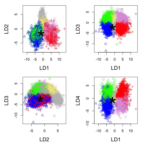
Figure 2: Human SNP data: projection of the reference table on the first four LDA axes. Colors correspond to model indices. The location of the additional datasets is indicated by a large black star.

ABC-RF algorithm selects Scenario 2 as the forecasted scenario on the Human dataset, an answer which is not visually obvious on the LDA projections of Figure 2, Scenario 2 corresponds to the blue color. But considering previous population genetics studies in the field, it is not surprising that this scenario, which includes a single out-of-Africa colonization event giving an ancestral out-of-Africa population with a secondarily split into one European and one East Asian population lineage and a recent genetic admixture of Americans of African origin with their African ancestors and European individuals, was selected. Using Algorithm 3, we got an estimate of the posterior probability of scenario 2 equal to $0.998$ which is as expected very high.

Computation time is a particularly important issue in the present example. Simulating the $10,000$ SNP datasets used to train the classification methods requires seven hours on a computer with 32 processors (Intel Xeon(R) CPU 2GHz). In that context, it is worth stressing that RF trained on the DIYABC summaries and the LDA axes of a $10,000$ reference table has a smaller prior error rate than all other classifiers, even when they are trained on a $50,000$ reference table. In practice, standard ABC treatments for model choice are based on reference tables of substantially larger sizes (i.e. $10^{5}$ to $10^{6}$ simulations per scenario (Estoup et al.,, 2012; Bertorelle et al.,, 2010)). For the above setting in which six scenarios are compared, standard ABC treatments would hence request a minimum computation time of 17 days (using the same computation resources). According to the comparative tests that we carried out on various example datasets, we found that RF globally allowed a minimum computation speed gain around a factor of 50 in comparison to standard ABC treatments.

3.4 Practical recommendations regarding the implementation of the algorithms

We develop here several points, formalized as questions, which should help users seeking to apply our methodology on their dataset for statistical model choice.

Are my models and/or associated priors compatible with the observed dataset?

This question is of prime interest and applies to any type of ABC treatment, including both standard ABC treatments and treatments based on ABC random forests. Basically, if none of the proposed model - prior combinations produces some simulated datasets in a reasonable vicinity of the observed dataset, it is a signal of incompatibility and we consider it is then useless to attempt model choice inference. In such situations, we strongly advise reformulating the compared models and/or the associated prior distributions in order to achieve some compatibility in the above sense. We propose here a visual way to address this issue, namely through the simultaneous projection of the simulated reference table datasets and of the observed dataset on the first LDA axes, such a graphical assessment can be achieved using the R package abcrf associated with this paper. In the LDA projection, the observed dataset need be located reasonably within the clouds of simulated datasets (see Figure 2 as an illustration). Note that visual representations of a similar type (although based on PCA) as well as computation for each summary statistics and for each model of the probabilities of the observed values in the prior distributions have been proposed by Cornuet et al., (2010) and are already automatically provided by the DIYABC software.

Did I simulate enough datasets for my reference table?

A rule of thumb is to simulate between 5,000 and 10,000 datasets per model among those compared. For instance, in the example dealing with Human population history (Section 3.3) we have simulated a total of 50,000 datasets from six models (i.e., about 8,300 datasets per model). To evaluate whether or not this number is sufficient for random forest analysis, we recommend to compute global prior error rates from both the entire reference table and a subset of the reference table (for instance from a subset of 40,000 simulated datasets if the reference table includes a total of 50,000 simulated datasets). If the prior error rate value obtained from the subset of the reference table is similar, or only lightly higher, than the value obtained from the entire reference table, one can consider that the reference table contains enough simulated datasets. If a substantial difference is observed between both values, then we recommend an increase in the number of datasets in the reference table. For instance, in the Human population history example we obtained prior error rate values of 4.22% and 4.18% when computed from a subset of 40,000 simulated datasets and the entire 50,000 datasets of the reference table, respectively. In this case, the hardship of producing more simulated dataset in the reference table seems negligible.

Did my forest grow enough trees?

According to our experience, a forest made of 500 trees usually constitutes (Breiman,, 2001) an interesting trade-off between computation efficiency and statistical precision. To evaluate whether or not this number is sufficient, we recommend to plot the estimated values of the prior error rate and/or the posterior probability of the best model as a function of the number of trees in the forest. The shapes of the curves provide a visual diagnostic of whether such key quantities stabilize when the number of trees tends to 500. We provide illustrations of such visual representations in the case of the example dealing with Human population history in Figure 3.

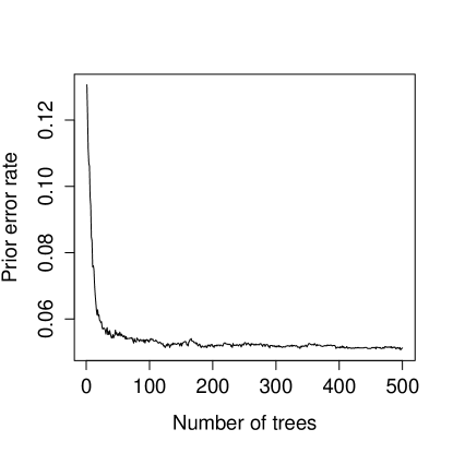
Figure 3: Human SNP data: evolution of the ABC-RF prior error rate when $N_{\text{ref}}=50,000$ with respect to the number of trees in the forest.

How do I set $N_{\text{boot}}$ and $N_{\text{try}}$? for classification and regression

For a reference table with up to 100,000 datasets and 250 summary statistics, we recommend keeping the entire reference table, that is, $N_{\text{boot}}=N$ when building the trees. For larger reference tables, the value of $N_{\text{boot}}$ can be calibrated against the prior error rate, starting with a value of $N_{\text{boot}}=50,000$ and doubling it until the estimated prior error rate is stabilized. For the number $n_{\text{try}}$ of summary statistics sampled at each of the nodes, we see no reason to modify the default number of covariates $n_{\text{try}}$ is chosen as $\sqrt{d}$ for classification and $d/3$ for regression when $d$ is the total number of predictors. Finally, when the number of summary statistics is lower than 15, one might reduce $N_{\text{boot}}$ to $N/10$.

4 Discussion

The present paper is purposely focused on selecting a statistical model, which can be rephrased as a classification problem trained on ABC simulations. We defend here the paradigm shift of assessing the best fitting model via a random forest classification and in evaluating our confidence in the selected model by a secondary random forest procedure, resulting in a different approach to precisely estimate the posterior probability of the selected model. We further provide a calibrating principle for this approach, in that the prior error rate provides a rational way to select the classifier and the set of summary statistics which leads to results closer to a true Bayesian analysis.

Compared with past ABC implementations, ABC-RF offers improvements at least at four levels: (i) on all experiments we studied, it has a lower prior error rate; (ii) it is robust to the size and choice of summary statistics, as RF can handle many superfluous statistics with no impact on the performance rates (which mostly depend on the intrinsic dimension of the classification problem (Biau,, 2012; Scornet et al.,, 2015), a characteristic confirmed by our results); (iii) the computing effort is considerably reduced as RF requires a much smaller reference table compared with alternatives (i.e., a few thousands versus hundred thousands to billions of simulations); and (iv) the method is associated with an embedded and free error evaluation which assesses the reliability of ABC-RF analysis. As a consequence, ABC-RF allows for a more robust handling of the degree of uncertainty in the choice between models, possibly in contrast with earlier and over-optimistic assessments.

Due to a massive gain in computing and simulation efforts, ABC-RF will extend the range and complexity of datasets (e.g. number of markers in population genetics) and models handled by ABC. In particular, we believe that ABC-RF will be of considerable interest for the statistical processing of massive SNP datasets whose production rapidly increases within the field of population genetics for both model and non-model organisms. Once a given model has been chosen and confidence evaluated by ABC-RF, it becomes possible to estimate parameter distribution under this (single) model using standard ABC techniques (Beaumont et al.,, 2002) or alternative methods such as those proposed by Excoffier et al., (2013).

5 Acknowledgments

The use of random forests was suggested to JMM and CPR by Bin Yu during a visit at CREST, Paris. We are grateful to G. Biau for his help about the asymptotics of random forests. Some parts of the research were conducted at BIRS, Banff, Canada, and the authors (PP and CPR) took advantage of this congenial research environment. This research was partly funded by the ERA-Net BiodivERsA2013-48 (EXOTIC), with the national funders FRB, ANR, MEDDE, BELSPO, PT-DLR and DFG, part of the 2012-2013 BiodivERsA call for research proposals.

Appendix

Appendix A Classification and regression methods

Classification methods aim at forecasting a variable $Y$ that takes values in a finite set, e.g. $\{1,\ldots,M\}$, based on a predicting vector of covariates $X=(X_{1},\ldots,X_{d})$ of dimension $d$. They are fitted with a training database $(x^{i},y^{i})$ of independent replicates of the pair $(X,Y)$. We exploit such classifiers in ABC model choice by predicting a model index ($Y$) from the observation of summary statistics on the data ($X$). The classifiers are trained with numerous simulations from the hierarchical Bayes model that constitute the ABC reference table. For a more detailed entry on classification, we refer the reader to the entry Hastie et al., (2009) and to the more theoretical Devroye et al., (1996).

On the other hand, regression methods forecast a continuous variable $Y$ based on the vector $X$. When trained on a database of independent replicates of a pair $(X,Y)$ with the $L^{2}$-loss, regression methods approximate the conditional expected value $\mathbb{E}(Y|X)$. A random forest for regression is used to obtain approximations of the posterior probability of the selected model.

A.1 Standard classifiers

Discriminant analysis covers a first family of classifiers including linear discriminant analysis (LDA) and naïve Bayes. Those classifiers rely on a full likelihood function corresponding to the joint distribution of $(X,Y)$, specified by the marginal probabilities of $Y$ and the conditional density $f(x|y)$ of $X$ given $Y=y$. Classification follows by ordering the probabilities $\text{Pr}(Y=y|X=x)$. For instance, linear discriminant analysis assumes that each conditional distribution of $X$ is a multivariate Gaussian distribution with unknown mean and covariance matrix, when the covariance matrix is assumed to be constant across classes. These parameters are fitted on a training database by maximum likelihood; see e.g. Chapter 4 of Hastie et al., (2009). This classification method is quite popular as it provides a linear projection of the covariates on a space of dimension $M-1$, called the LDA axes, which separate classes as much as possible. Similarly, naïve Bayes assumes that each density $f(x|y)$, $y=1,\ldots,M$, is a product of marginal densities. Despite this rather strong assumption of conditional independence of the components of $X$, naïve Bayes often produces good classification results. Typically we assume that the marginals are univariate Gaussians and fit those by maximum likelihood estimation.

Logistic and multinomial regressions use a conditional likelihood based on a modeling of $\text{Pr}(Y=y|X=x)$, as special cases of a generalized linear model. Modulo a logit transform $\phi(p)=\log\{p/(1-p)\}$, this model assume linear dependency in the covariates; see e.g. Chapter 4 in Hastie et al., (2009). Logistic regression results rarely differ from LDA estimates since the decision boundaries are also linear. The sole difference stands with the procedure used to fit the classifiers.

A.2 Local classification methods

$k$-nearest neighbor ($k$-nn) classifiers require no model fitting but mere computations on the training database. More precisely, it builds upon a distance on the feature space, $\mathcal{X}\ni X$. In order to make a classification when $X=x$, $k$-nn derives the $k$ training points that are the closest in distance to $x$ and classifies this new datapoint $x$ according to a majority vote among the classes of the $k$ neighbors. The accuracy of $k$-nn heavily depends on the tuning of $k$, which should be calibrated, as explained below.

Local logistic (or multinomial) regression adds a linear regression layer to these procedures and dates back to Cleveland, (1979). In order to make a decision at $X=x$, given the $k$ nearest neighbors in the feature space, one weights them by a smoothing kernel (e.g., the Epanechnikov kernel) and a multinomial classifier is then fitted on this weighted sub-sample of the training database. More details on this procedure can be found in Estoup et al., (2012). Likewise, the accuracy of the classifier depends on the calibration of $k$.

A.3 Randomized CART

The Random Forest (RF) algorithm aggregates randomized Classification And Regression Trees (CART), which can be trained for both classification and regression issues. The randomized CART algorithm used to create the trees in the forest recursively infers the internal and terminal labels of each tree $i$ from the root on a training database $(x^{i},y^{i})$ as follows. Given a tree built until a node $v$, daughter nodes $v_{1}$ and $v_{2}$ are determined by partitioning the data remaining at $v$ in a way highly correlated with the outcome $Y$. Practically, this means minimizing an empirical divergence criterion towards selecting the best covariate $X_{j}$ among a random subset of size $n_{\text{try}}$ and the best threshold $t$. The covariate $X_{j}$ and the threshold $t$ is determined by minimizing $N(v_{1})Q(v_{1})+N(v_{2})Q(v_{2})$, where $N(v_{i})$ is the number of records from the training database that fall into node $v_{i}$ and $Q(v_{i})$ is the empirical criterium at node $v_{i}$. For regression, we used the $L^{2}$-loss. For classification, we privileged the Gini index, defined as

$$Q(v_{i})=\sum_{y=1}^{M}\hat{p}(v_{i},y)\left\{1-\hat{p}(v_{,}y)\right\}\,,$$

where $\hat{p}(v_{i},y)$ is the relative frequency of $y$ among the part of the learning database that falls at node $v_{i}$. Other criteria are possible, see Chapter 9 in Hastie et al., (2009).

For regression, the recursive algorithm stops when all terminal nodes $v$ correspond to at most five records of the training database, and the label of the tip $v$ is the average of $y$ over these five records. For classification, it stops when the terminal nodes are homogeneous, i.e., $Q(v)=\sum_{y=1}^{M}\hat{p}(v,y)\{1-\hat{p}(v,y)\}=0$ and the label of the tip $v$ is the only value of $y$ for which $\hat{p}(v,y)=1$. This leads to Algorithm S1.

Algorithm S1: Randomized CART

  start the tree with a single root

  repeat

     pick a non-homogeneous tip $v$ such that $Q(v)>0$ (classification) or $N(v)>5$ (regression)

     attach to $v$ two daughter nodes $v_{1}$ and $v_{2}$

     draw a random subset of covariates of size $n_{\text{try}}$

     for all covariates $X_{j}$ in the random subset do

        find the threshold $t_{j}$ in the rule $X_{j}<t_{j}$ that minimizes $N(v_{1})Q(v_{1})+N(v_{2})Q(v_{2})$

     end for

     find the rule $X_{j}<t_{j}$ that minimizes $N(v_{1})Q(v_{1})+N(v_{2})Q(v_{2})$ in $j$

     and set this best rule to node $v$

  until all tips $v$ are homogeneous (classification) or correspond to 5 records (regression)

  set the labels of all tips

A.4 Calibration of the tuning parameters

Many machine learning algorithms involve tuning parameters that need to be determined carefully in order to obtain good results (in terms of what is called the prior error rate in the main text). Usually, the predictive performances (averaged over the prior in our context) of classifiers are evaluated on new data (validation procedures) or fake new data (cross-validation procedures); see e.g. Chapter 7 of Hastie et al., (2009). This is the standard way to compare the performances of various possible values of the tuning parameters and thus calibrate these parameters. For instance, the value of $k$ for both $k$-nn and local logistic regression need to be calibrated. $k$-nn performances heavily depend on the value of $k$ as illustrated on Figure A.4. The plots in this Figure display an empirical evaluation of the prior error rates of the classifiers against different values of their tuning parameter with a validation sample made of a fresh set of $10^{4}$ simulations from the hierarchical Bayesian model. Because of the moderate Monte Carlo noise within the empirical error, we first smooth out the curve before determining the calibration of the algorithms. Figure A.4 displays this derivation for the ABC analysis of the Harlequin ladybird data with machine learning tools.

The validation procedure described above requires new simulations from the hierarchical Bayesian model, which we can always produce because of the very nature of ABC. But such simulations might be computationally intensive when analyzing large datasets or complex models. Moreover, calibrating local logistic regression may prove computationally unfeasible since for each dataset of the validation sample (the second reference table), the procedure involves searching for nearest neighbors in the (first) reference table, then fitting a weighted logistic regression on those neighbors.

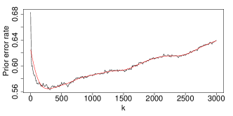
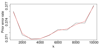
Figure 4: Calibration of $k$-nn, the local logistic regression. Plot of the empirical prior error rate (in black) of three classifiers, namely $k$-nn (left), the local logistic regression (right) as a function of their tuning parameter when analyzing the Harlequin ladybird data with a reference table of $10,000$ simulations. To remove the noise of these estimated errors on a validation set composed of $10,000$ independent simulations, estimated errors are smoothed by a spline method that produces the red curve. The optimal values of the parameters are $k=300$ and $k=3,000$ respectively.

Appendix B A revealing toy example: MA(1) versus MA(2) models

Given a time series $(x_{t})$ of length $T=100$, we compare fits by moving average models of order either $1$ or $2$, MA(1) and MA(2), namely

$$x_{t}=\epsilon_{t}-\theta_{1}\epsilon_{t-1}\ \text{and}\ x_{t}=\epsilon_{t}-\theta_{1}\epsilon_{t-1}-\theta_{2}\epsilon_{t-2}\,,\ \epsilon_{t}\sim\text{N}(0,\sigma^{2})\,,$$

respectively. As previously suggested Marin et al., (2012), a possible set of (insufficient) summary statistics is made of the first seven autocorrelations, set that yields an ABC reference table of size $N_{\text{ref}}=10^{4}$ with seven covariates. For both models, the priors are uniform distributions on the stationarity domains Robert, (2001):

• for MA(1), the single parameter $\theta_{1}$ is drawn uniformly from the segment $(-1;1)$;

• for MA(2), the pair $(\theta_{1},\theta_{2})$ is drawn uniformly over the triangle defined by

  $$-2<\theta_{1}<2,\quad\theta_{1}+\theta_{2}>1,\quad\theta_{1}-\theta_{2}<1.$$

In this example, we can evaluate the discrepancy between the posterior probabilities based on the whole data and those based on summaries. We first consider as summary statistics the first two autocorrelations that are very informative for this problem. The marginal likelihoods based on the whole data can be computed by numerical integrations of dimension $1$ and $2$ respectively, while the ones based on the summary statistics are derived from a well-adapted kernel smoothing method. Figure 1 of the main text shows how different the posterior probabilities are when based on (i) the whole series of length $T=100$ and (ii) only the first two autocorrelations, even though the latter remain informative about the problem. This graph brings numerical support to the severe warnings of Robert et al., (2011).

Moreover, Table B draws a comparison between various classifiers when we consider as summary statistics the first seven autocorrelations. All methods based on summaries are outperformed by the Bayes classifier that can be computed here via approximations of the genuine $\pi(m|x)$: this ideal classifier achieves a prior error of around $12\%$. The RF classifier achieves the minimum with a prior error rate of around $16\%$.

If we now turn to the performances of the second random forest to evaluate the posterior probability of the selected model (computed with Algorithm 3 displayed in the main text), Figure B shows how the evaluation of the posterior probability of the model selected by Algorithm 3 vary when compared to the true posterior probability of the selected model. When the true posterior probability of the selected model is high, Algorithm 3 has a tendency to underestimate the probability. Another important feature is that this approximation of the posterior probability do not provide any warning regarding a decision swap between the true MAP model and the model selected by Algorithm 2: see the black dots of Figure B.

Classification method	Prior error rate (%)
Linear discriminant analysis (LDA)	$26.57$
Logistic regression	$27.40$
Naïve Bayes	$24.40$
$k$-nn with $k=100$ neighbors	$18.37$
$k$-nn with $k=50$ neighbors	$17.35$
Random forests	$16.15$

Table 3: Estimated prior error rates in the MA(1) vs. MA(2) example. The prior error rates displayed here were computed as averaged misclassification errors on a set of $10^{4}$ simulations independent of the simulation set of $10^{4}$ values that trained the classifiers. Summary statistics are the first seven autocorrelations. A baseline error of $12.36\%$ is obtained when comparing the genuine posterior probabilities on the whole data.

Figure 5: Posterior probability of the selected model in the MA(1) vs. MA(2) example. The graph compares the true posterior probabilities (x-axis) of the decision taken by Algorithm 2 on 1,000 simulated time series with the approximation of these probabilities (y-axis) provided by Algorithm 3. For each time series, the decision taken by Algorithm 2 can agree with the true model index that has MAP probability: dots are blue when both are in favor of the MA(1) model, orange when in favor of the MA(2) model. Black dots represents simulated time series which leads to a discrepancy between both decisions.

Appendix C Examples based on controlled simulated population
genetic datasets

We now consider a basic population genetic setting ascertaining historical links between three populations of a given species. In both examples below, we try to decide whether a third (and recent) population emerged from a first population (Model 1), or from a second population that split from the first one some time ago (Model 2), or whether this third population was a mixture between individuals from both populations (Model 3); see Figure C.

Figure 6: Three competing models of historical relationships between populations of a given species. Those population models or scenarios are used for both controlled examples based on SNP and microsatellite data: (left) Model 1 where Population 3 split from Population 1, (center) Model 2 where Population 3 split from Population 2, (right) Model 3 where Population 3 is an admixture between Populations 1 and 2. Branches in blue represent population of effective size $N_{1}$, in green $N_{2}$, in red $N_{3}$ and in cyan $N_{4}$.

The only difference between both examples stands with the kind of data they consider: the $1,000$ genetic markers of the first example are autosomal, single nucleotide polymorphims (SNP) loci and the $20$ markers of the second example are autosomal microsatellite loci. We assume that, in both cases, the data were collected on samples of 25 diploid individuals from each population. Simulated and observed genetic data are summarized with the help of a few statistics described in Section G of the appendix. They are all computable with the DIYABC software Cornuet et al., (2014) that we also used to produce simulated datasets; see also Section F below.

For both examples, the seven demographics parameters of the Bayesian model are

• $t_{S}$: time of the split between Populations 1 and 2,

• $t_{A}$: time of the appearance of Population 3,

• $N_{1}$, $N_{2}$, $N_{3}$: effective population sizes of Populations 1, 2 and 3, respectively, below time $t_{S}$,

• $N_{4}$: effective population size of the common ancestral population above $t_{S}$ and

• $r$: the probability that a gene from Population 3 at time $t_{A}$ came from Population 1.

This last parameter $r$ is the rate of the admixture event at time $t_{A}$ and as such specific to Model 3. Note that Model 3 is equivalent to Model 1 when $r=1$ and to Model 2 when $r=0$. But the prior we set on $r$ avoids nested models. Indeed, the prior distribution is as follows:

• the times $t_{S}$ and $t_{A}$ (on the scale of number of generations) are drawn from a uniform distribution over the segment $[10;\ 3\times 10^{4}]$ conditionally on $t_{A}<t_{S}$;

• the four effective population sizes $N_{i}$, $i=1,\ldots,4$ are drawn independently from a uniform distribution on a range from $100$ to $30,000$ diploid individuals, denoted $U(100;3\times 10^{4})$;

• the admixture rate $r$ is drawn from a uniform distribution $U(0.05;\ 0.95)$.

In this example, the prior on model indices is uniform so that each of the three models has a prior probability of $1/3$.

C.1 SNP data

The data is made of $1,000$ autosomal SNPs for which we assume that the distances between these loci on the genome are large enough to neglect linkage disequilibrium and hence consider them as having independent ancestral genealogies. We use all summary statistics offered by the DIYABC software for SNP markers Cornuet et al., (2014), namely 48 summary statistics in this three population setting (provided in Section G of the appendix). In total, we simulated $70,000$ datasets, based on the above priors. These datasets are then split into three groups:

• $50,000$ datasets constitute the reference table and reserved for training classification steps, (we will also consider classifiers trained on subsamples of this set),

• $10,000$ datasets constitute the validation set, used to calibrate the tuning parameters of the classifiers if needed, and

• $10,000$ datasets constitute the test set, used to evaluating the prior error rates.

The classification methods applied here are given in Table C.2. For the naïve Bayes classifier and the LDA procedures, there is no parameter to calibrate. This is also the case of the RF methods that, for such training sample sizes, do not require any calibration for $N_{\text{boot}}$. The numbers $k$ of neighbors for the standard ABC techniques and for the local logistic regression are tuned as described in Section A above.

The prior error rates are estimated and minimized by using the validation set of $10^{4}$ simulations, independent from the reference table. The optimal value of $k$ for the standard ABC ($k$-nn) and 48 summary statistics is small because of the dimension of the problem ($k=9$, $k=15$, and $k=55$ when using $10,000$, $20,000$ and $50,000$ simulations in the reference table respectively). The optimal values of $k$ for the local logistic regression are different, since this procedure fits a linear model on weighted neighbors. The calibration on a validation set made of $10,000$ simulations produced the following optimal values: $k=2,000$, $k=3,000$, and $k=6,000$ when fitted on $10,000$, $20,000$, and $50,000$ simulations, respectively. As reported in Section A above, calibrating the parameter $k$ of the local logistic regression is very time consuming. For the standard ABC ($k$-nn) based on original summaries, we relied on a standard Euclidean distance after normalizing each variable by its median absolute deviation, while $k$-nn on the LDA axes requires no normalization procedure.

Table C.2 provides estimated prior error rates for those classification techniques, based on a test sample of $10,000$ values, independent of reference tables and calibration sets. It shows that the best error rate is associated with a RF trained on both the original DIYABC statistics and the LDA axes. The gain against the standard ABC solution is clearly significant. Other interesting features exhibited in Table C.2 are (i) good performances of the genuine LDA method, due to a good separation between summaries coming from the three models, as exhibited in Figure C.2, albeit involving some overlap between model clusters, (ii) that the local logistic regression on the two LDA axes of Estoup et al., (2012) achieves the second best solution.

Figure C.2 describes further investigations into the RF solution. This graph expresses the contributions from the summary statistics to the decision taken by RF. The contribution of each summary is evaluated as the average decrease in the Gini criterium over the nodes driven by the corresponding summary statistic, see e.g. Chapter 15 of Hastie et al., (2009). The appeal of including the first two LDA axes is clear in Figure C.2, where they appear as LD1 and LD2: those statistics contribute more significantly than any other statistic to the decision taken by the classifier. Note that the FMO statistics, which also have a strong contribution to the RF decisions, are the equivalent of pairwise $F_{ST}$-distances between populations when genetic markers are SNPs. The meaning of the variable acronyms is provided in Section G below.

We simulated two typical datasets, hereafter considered as pseudo-observed datasets or pod(s). The first pod (green star in Figure C.2) corresponds to a favorable situation for which Model 3 should easily be discriminated from both Models 1 and 2. The parameter values used to simulate this pod indeed correspond to a recent balanced admixture between strongly differentiated source populations ($N_{1}=20,000$, $N_{2}=15,000$, $N_{3}=10,000$, $N_{4}=25000$, $r=0.5$, $t_{a}=500$ and $t_{s}=20000$). The second pod (red star in Figure C.2) corresponds to a less favorable setting where it is more difficult to discriminate Model 3 from Model 1 and 2. The parameter values used to simulate this second pod correspond to an ancient unbalanced admixture between the source populations ($N_{1}=20,000$, $N_{2}=15,000$, $N_{3}=10,000$, $N_{4}=25,000$, $r=0.1$, $t_{a}=10,000$, and $t_{s}=20,000$).

For both pods, ABC-RF (trained on both the 48 initial statistics and the two LDA axes) chooses Model 3. The RF was trained on a reference table of size $70,000$ (that contains all simulations). The first pod is allocated to Model 3 for all the 500 trees in the forest while the second pod is allocated to Model 3 for 261 trees (238 for Model 2 and only 1 for Model 1). As already explained, these numbers are very variable and does not represent valid estimations of the posterior probabilities. The regression RF evaluation of the posterior probabilities of the selected model (Model 3), based on 500 trees and using the 0-1 error vector (of size 70,000), are substantially different for both pods: very close to $1$ for the first one and about $0.756$ for the second. These posterior probabilities can be compared to the $17.9\%$ out-of-bag estimation of the prior error rate. Indeed, the first pod is attributed to Model 3 with an error close to zero and the second one with an error about $24.6\%$. That is totally in agreement with the position of the pods represented by the green and red stars in Figure C.2. The second pod belongs to a region of the data space where it seems difficult to discriminate between Models 2 and 3.

C.2 Microsatellite data

This illustration reproduces the same settings as in the SNP data example above but the genetic data (which is of much smaller dimension) carries a different and lower amount of information. Indeed, we consider here datasets composed of only 20 autosomal microsatellite loci. The microsatellite loci are assumed to follow a generalized stepwise mutation model with three parameters Estoup et al., (2002); Lombaert et al., (2011): the mean mutation rate ($\bar{\mu}$), the mean parameter of the geometric distribution ($\bar{P}$) of changes in number of repeats during mutation events, and the mean mutation rate for single nucleotide instability ($\overline{\mu_{SNI}}$). The prior distributions for $\bar{\mu}$, $\bar{P}$ and $\overline{\mu_{SNI}}$ are the same as those given in Table 1 (see the prior distributions used for the real Harmonia axyridis microsatellite dataset). Each locus has a possible range of 40 contiguous allelic states and is characterized by locus specific $\mu$’s drawn from a Gamma distribution with mean $\bar{\mu}$ and shape $2$, locus specific $P$’s drawn from a Gamma distribution with mean $\bar{P}$ and shape $2$ and, finally, locus specific $\mu_{\text{SNI}}$’s drawn from a Gamma distribution with mean $\overline{\mu_{SNI}}$ and shape $2$. For microsatellite markers, DIYABC (Cornuet et al.,, 2014) produces 39 summary statistics described in Section G below.

Table C.2 is the equivalent of Table C.2 for this kind of genetic data structure. Due to the lower and different information content of the data, the prior error rates are much higher in all cases, but the conclusion about the gain brought by RF using all summaries plus the LDA statistics remains.

As in the SNP case, we simulated two typical pods: one highly favorable (the green star in Figure C.2) and a second one quite challenging (the red star in Figure C.2). They were generated using the same values of parameters as for the SNP pods.

For both pods, we considered an ABC-RF treatment with a reference table of size $70,000$. The first pod is allocated to Model 3: 491 trees associate this dataset to Model 3, 3 to Model 1 and 6 to Model 2. The second pod is also allocated to Model 3: 234 trees associate this dataset to Model 3, 61 to Model 1 and 205 to Model 2. We run a regression RF model to estimate the corresponding posterior probabilities. Using once again 500 trees and the $70,000$ 0-1 error vector we obtained about $0.996$ for the first pod and about $0.598$ for the more challenging one. We hence got for the challenging pod a classification error (1 minus the posterior probability of the selected model) that is larger than the prior error rate.

Interestingly Figure C.2 shows that the AML_3_1&2 summary statistic (see Section G below) contributes more to the RF decision than the second LDA axis. We recall that AML is an admixture rate estimation computed by maximum likelihood on a simplified model considering that the admixture occurred at time $t=0$. The importance of the LDA axes in the random forest remains nevertheless very high in this setting.

Figure 7: Projections on the LDA axes of the simulations from the reference table for the controlled SNP example. Colors correspond to model indices: black for Model 1, blue for Model 2 and orange for Model 3. The locations of both simulated pseudo-observed datasets that are analyzed as if they were truly observed data, are indicated by green and red stars.

Figure 8: Contributions of the twenty most important statistics to the RF for the controlled SNP example. The contribution of a statistic is evaluated as the mean decrease in the Gini criterium when using 48 summary statistics (top) and when adding the two LDA axes to the previous set of statistics (bottom).

Figure 9: Projections on the LDA axes of the simulations from the reference table for the controlled microsatellite example Colors correspond to model indices: black for Model 1, blue for Model 2 and orange for Model 3. The locations of both simulated pseudo-observed datasets are indicated by green and red stars.

Figure 10: Contributions of the twenty most important statistics to the RF for the controlled microsatellite example. The contribution of a statistic is evaluated with the mean decrease in the Gini criterium when using 39 summary statistics (top) and when adding the two LDA axes to the previous set of statistics (bottom).

Classification method	Prior error rates (%)
trained on	$N_{\text{ref}}=10,000$	$N_{\text{ref}}=20,000$	$N_{\text{ref}}=50,000$
Naïve Bayes (with Gaussian marginals)	$34.86$	$34.72$	$34.41$
Linear discriminant analysis (LDA)	$23.35$	$23.28$	$23.12$
Standard ABC ($k$-nn) using DIYABC summaries	$27.82$	$25.61$	$23.58$
Standard ABC ($k$-nn) using only LDA axes	$22.86$	$22.56$	$22.60$
Local logistic regression on LDA axes	$22.07$	$21.84$	$21.93$
RF using DIYABC initial summaries	$22.13$	$20.71$	$19.55$
RF using both DIYABC summaries and LDA axes	$20.07$	$18.95$	$18.11$

Table 4: Estimated prior error rates for the controlled SNP example.

Classification method	Prior error rates (%)
trained on	$N_{\text{ref}}=10,000$	$N_{\text{ref}}=20,000$	$N_{\text{ref}}=50,000$
Naïve Bayes (with Gaussian marginals)	$40.41$	$40.74$	$40.43$
Linear discriminant analysis (LDA)	$36.54$	$36.49$	$36.47$
Standard ABC ($k$-nn) using DIYABC summaries	$39.23$	$38.37$	$36.99$
Standard ABC ($k$-nn) using only LDA axes	$37.17$	$36.93$	$36.05$
Local logistic regression on LDA axes	$36.11$	$35.93$	$35.89$
RF using DIYABC initial summaries	$37.07$	$36.16$	$35.32$
RF using both DIYABC summaries and LDA axes	$35.53$	$35.32$	$34.38$

Table 5: Estimated prior error rates for the controlled microsatellite example.

Appendix D Supplementary informations about
the Harlequin ladybird example

Reconstructing the history of the invasive populations of a given species is crucial for both management and academic issues Estoup and Guillemaud, (2010). The real dataset analyzed here and in the main text relates to the recent invasion history of a coccinellidae, Harmonia axyridis. Native from Asia, this insect species was recurrently introduced since 1916 in North America as a biocontrol agent against aphids. It eventually survived in the wild and invaded four continents. The present dataset more specifically aims at making inference about the introduction pathway of the invasive H. axyridis for the first recorded outbreak of this species in eastern North America, which corresponds to a key introduction event in the worldwide invasion history of the species. We refer the reader to Estoup and Guillemaud, (2010) and Lombaert et al., (2011) for more details on the biological issues associated to the situation considered and for a previous statistical analysis based on standard ABC techniques.

Using standard ABC treatments, Lombaert et al., (2011) formalized and compared ten different scenarios (i.e., models) to identify the source population(s) of the eastern North America invasion (see Figure D for a graphical representation of a typical invasion scenario and Table D for parameter prior distributions). We now compare our results based on the ABC-RF algorithm with this original paper, as well as with other classification methods. The H. axyridis dataset is made of samples from five populations comprising 35, 18, 34, 26 and 25 diploid individuals, genotyped at 18 autosomal microsatellite loci considered as selectively neutral and statistically independent markers. The problem we face is considerably more complex than the above controlled and simulated population genetic illustrations in that the numbers and complexity levels of both competing models and sampled populations are noticeably higher. Since the summary statistics proposed by DIYABC Cornuet et al., (2014) describe features that operate per population, per pair, or per triplet of populations, averaged over the 18 loci, we can include up to 130 of those statistics plus the nine LDA axes as summary statistics in our ABC-RF analysis. The gap in the dimension of the summary statistics is hence major when compared with the 48 and 39 sizes in the previous sections. The ABC-RF computations to discriminate among the ten scenarios and evaluate error rates were processed on 10,000, 20,000, and 50,000 datasets simulated with DIYABC; see Section 7 below and Cornuet et al., (2014). It is worth noting here that the standard ABC treatments processed in Lombaert et al., (2011) on the same dataset relied on a set of 86 summary statistics which were selected thanks to the author expertise in population genetic model choice, as well as on a substantially larger number of simulated datasets (i.e., $1,000,000$ per scenario). Compared to the standard ABC treatments processed in Lombaert et al., (2011), ABC-RF computation allowed substantial computation speed: a factor 200 to 1000 for the simulation of the reference table.

Figure 11: Projections on the first four LDA axes of simulations from the reference table of the Harlequin ladybird analysis. Colors correspond to model indices. The location of the real observed dataset for the Harlequin ladybird is indicated by a black star.

Figure 12: Contributions of the most important statistics to the RF for the Harlequin ladybird example. The contribution of a statistic is evaluated with the mean decrease in node impurity in the trees of the RF when using 130 summary statistics (top) and when adding the nine LDA axes to the previous set of statistics (bottom). The meaning of the variable acronyms is provided in Appendix S2.

Figure 13: Representation of the invasion scenario of the Harlequin ladybird that was selected among ten scenarios when using either the proposed ABC-RF method or the standard ABC analysis processed in Lombaert et al., (2011). Population names between brackets correspond to sample names in Lombaert et al., (2011). Populations (i.e., Pop) 1 and 2 are native populations; Pop 3 is the target invasive population for which one wants to make inference about the source population(s) (here Pop 3 is an admixture between the source populations Pop 1 and Pop 2); Pop 4 and 5 are biocontrol populations; Pop ubc6 and ubc7 are unsampled biocontrol populations. Time 0 is the sampling date of Pop 1, 2 and 3. Time 50 and time 67 are the sampling dates of Pop 4 and 5 respectively. Dashed lines correspond to unsampled native populations; see Lombaert et al., (2011) for a comprehensive explanation of this design. Populations were assumed to be isolated from each other, with no exchange of migrants. All parameters are described with their associated prior in Table 1. This scenario was opposed to nine competing scenarios corresponding to alternative single or multiple source(s) for the introduced target population Pop 3; see Lombaert et al., (2011) for details.

parameter	prior
$\text{NS}_{i}$, $\text{NS}_{j}$	$\mathcal{U}(100,20000)$
$\log(\text{NS}_{k})$	$\mathcal{U}(10,10^{4})$
$\log(\text{NF}_{i})$	$\mathcal{U}(2,10^{4})$
$\text{BD}_{i}$	$\mathcal{U}(0,5)$
ar	$\mathcal{U}(0.1,0.9)$
$t_{i}$, $t_{k}$	$\mathcal{U}(x_{i},x_{i}+5)$
$\log(tbc_{i})$	$\mathcal{U}(t_{i},93)$
$\log(tu_{ji})$, $\log(tu_{jk})$	$\mathcal{U}(tbc_{i},3000)$
$t_{\text{anc}}$	$\mathcal{U}(100,3000)$
$\bar{\mu}$	$\mathcal{U}(10^{-5},10^{-3})$
$\bar{P}$	$\mathcal{U}(0.1,0.3)$
$\overline{\mu_{\text{SNI}}}$	$\mathcal{U}(10^{-8},10^{-4})$

Table 6: Prior distributions of demographic, historical, and mutation parameters used to simulate microsatellite datasets and corresponding summary statistics under the ten invasion scenarios of Harlequin ladybird. Prior distributions are the same as those used in Lombaert et al., (2011) and Estoup et al., (2012). Populations $i$ are invasive populations, clusters $j$ are native population clusters (either Western Asia or Eastern Asia cluster) and populations $k$ correspond to biocontrol strains (i.e., laboratory reared populations). Times were translated into numbers of generations running back in time and assuming 2.5 generations per year, $NS$ stands for stable effective population size (number of diploid individuals); $NF$ for effective number of founders during an introduction step lasting BD generation(s); $ar$ for admixture rate (only for scenarios with admixture); $t_{i}$ for introduction date of invasive populations $i$ with limits $x_{i}$ fixed from dates of first observation, assuming 2.5 generations per year; $t_{k}$ for sampling date in the native area of biocontrol population $k$ with limits $x_{i}$ fixed from historical information, assuming 2.5 generations per year; $tbc_{i}$ for creation date of unsampled biocontrol strain for Eastern and Western North America populations bounded by the dates of the first observation of the invasive population (corresponding to a direct introduction into the wild) and the number of generations from 1970, the starting date of a period of intense H. axyridis biocontrol activity in the USA; $tu_{j}$ for native cluster $j$ date of merging of the source unsampled native population with the sampled native population (this parameter is included in the model in which the scenario contains one or both native populations as possible source(s) of population $i$ or population $k$); $t_{\text{anc}}$ for the date of the merging of the two native populations into an ancestral unsampled population (with condition $tu_{j}\leq t_{\text{anc}}$). See Lombaert et al., (2011) and Estoup et al., (2012) for additional details.

Appendix E Supplementary informations about
the Human population example

We here illustrate the potential of our ABC-RF algorithm for the statistical processing of massive single nucleotide polymorphism (SNP) datasets, whose production is on the increase within the field of population genetics. To this aim, we analyzed a SNP dataset obtained from individuals originating from four Human populations (30 unrelated individuals per population) using the freely accessible public 1000 Genome databases (i.e., the vcf format files including variant calls available at http://www.1000genomes.org/data). The goal of the 1000 Genomes Project is to find most genetic variants that have frequencies of at least 1% in the studied populations by sequencing many individuals lightly (i.e., at a $4\times$ coverage). A major interest of using SNP data from the 1000 Genomes Project The 1000 Genomes Project Consortium, (2012) is that such data does not suffer from any ascertainment bias (i.e., the deviations from expected theoretical results due to the SNP discovery process in which a small number of individuals from selected populations are used as discovery panel), which is a prerequisite when using the DIYABC simulator of SNP data Cornuet et al., (2014). The four Human populations included the Yoruba population (Nigeria) as representative of Africa (encoded YRI in the 1000 genome database), the Han Chinese population (China) as representative of the East Asia (encoded CHB), the British population (England and Scotland) as representative of Europe (encoded GBR), and the population composed of Americans of African ancestry in SW USA (encoded ASW). The SNP loci were selected from the 22 autosomal chromosomes using the following criteria: (i) all $30\times 4$ analyzed individuals have a genotype characterized by a quality score $(GQ)>10$ (on a PHRED scale), (ii) polymorphism is present in at least one of the $30\times 4$ individuals in order to fit the SNP simulation algorithm of DIYABC Cornuet et al., (2014), (iii) the minimum distance between two consecutive SNPs is 1 kb in order to minimize linkage disequilibrium between SNPs, and (iv) SNP loci showing significant deviation from Hardy-Weinberg equilibrium at a 1% threshold Wigginton et al., (2005) in at least one of the four populations have been removed (35 SNP loci involved). After applying the above criteria, we obtained a dataset including 51,250 SNP loci scattered over the 22 autosomes (with a median distance between two consecutive SNPs equal to 7 kb) among which 50,000 were randomly chosen for applying the proposed ABC-RF methods.

In this application, we compared six scenarios (i.e., models) of evolution of the four Human populations genotyped at the above mentioned 50,000 SNPs. The six scenarios differ from each other by one ancient and one recent historical event: (i) A single out-of-Africa colonization event giving an ancestral out-of-Africa population which secondarily splits into one European and one East Asia population lineage, versus two independent out-of-Africa colonization events, one giving the European lineage and the other one giving the East Asia lineage. The possibility of a second ancient (i.e., $>100,000$ years) out-of-Africa colonization event through the Arabian peninsula toward Southern Asia has been suggested by archaeological studies, e.g. Rose et al., (2011); (ii) The possibility (or not) of a recent genetic admixture of Americans of African ancestry in SW USA between their African ancestors and individuals of European or East Asia origins.

The six different scenarios as well as the prior distributions of the time event and effective population size parameters used to simulate SNP datasets using DIYABC are detailed in Figure E. We stress here that our intention is not to bring new insights into Human population history, which has been and is still studied in greater details in a number of studies using genetic data, but to illustrate the potential of the proposed ABC-RF methods for the statistical processing of large size SNP datasets in the context of complex evolutionary histories. RF computations to discriminate among the six scenarios of Figure E and evaluate error rates were processed on 10,000, 20,000, and 50,000 simulated datasets. We used all summary statistics offered by the DIYABC software for SNP markers Cornuet et al., (2014) (see Section G below), namely 130 summary statistics in this setting plus the five LDA axes as additional summary statistics.

Figure 14: Contributions of the most important statistics to the RFs (to analyze the Human data). The contribution of a statistic is evaluated with the mean decrease in node impurity in the trees of the RF when using the 112 summary statistics (top) and when adding the five LDA axes to the previous set of statistics (bottom) . The meaning of the variable acronyms is provided in Appendix S1.

Figure 15: Six scenarios of evolution of four Human populations genotyped at 50,000 SNPs. The genotyped populations are YRI = Yoruba (Nigeria, Africa), CHB = Han (China, East Asia), GBR = British (England and Scotland, Europe), and ASW = Americans of African ancestry (SW USA). The six scenarios differ from each other by one ancient and one recent historical event: (i) a single out-of-Africa colonization event giving an ancestral out-of-Africa population which secondarily splits into one European and one East Asia population lineage (scenarios 1, 2 and 3), versus two independent out-of-Africa colonization events, one giving the European lineage and the other one giving the East Asia lineage (scenarios 4, 5 and 6). (ii) The possibility (or not; scenarios 1 and 4) of a recent genetic admixture of ASW individuals with their African ancestors and individuals of European (scenarios 2 and 5) or East Asia origins (scenarios 3 and 6). The prior distributions of the parameters used to simulate SNP datasets are as followed: Uniform[100; 10000] for the split times t2 and t3 (in number of generations), Uniform[1; 30] for the admixture (or split) time t1, Uniform[0.05; 0.95] for the admixture rate ra (proportion of genes with a non-African origin; only for scenarios with admixture), Uniform[1000; 100000] for the stable effective population sizes N1, N2, N4, N4 and N34 (in number of diploid individuals), Uniform[5; 500] for the bottleneck effective population sizes Nbn3, Nbn4, and Nbn34, Uniform[5; 500] for the bottleneck durations d3, d4, and d34, Uniform[100; 10000] for both the ancestral effective population size Na and the time of change to Na. Conditions on time events were t4$>$t3$>$t2 for scenarios 1, 2 and 3, and t4$>$t3 and t4$>$t2 for scenarios 4, 5 and 6.

Appendix F Computer software and codes

For all illustrations based on genetic data, we used the program DIYABC v2.0 (Cornuet et al.,, 2014) to generate the ABC reference tables including a set of simulation records made of model indices, parameter values and summary statistics for the associated simulated data. DIYABC v2.0 is a multithreaded program which runs on three operating systems: GNU/Linux, Microsoft Windows and Apple Mac Os X. Computational procedures are written in C++ and the graphical user interface is based on PyQt, a Python binding of the Qt framework. The program is freely available to academic users with a detailed notice document, example projects, and code sources (Linux) from: http://www1.montpellier.inra.fr/CBGP/diyabc. The reference table generated this way then served as training database for the random forest constructions. For a given reference table, computations were performed using the R package randomForest Liaw and Wiener, (2002). We have implemented all the proposed methodologies in the R package abcrf available on the CRAN.

Appendix G Summary statistics available in the DIYABC software

G.1 DIYABC summary statistics on SNP data

Single population statistics
HP0_i: proportion of monomorphic loci for population i
HM1_i: mean gene diversity across polymorphic loci (Nei,, 1987)
HV1_i: variance of gene diversity across polymorphic loci
HMO_i: mean gene diversity across all loci

Two population statistics
FP0_i&j: proportion of loci with null FST distance between the two samples for populations i and j (Weir and Cockerham,, 1984)
FM1_i&j: mean across loci of non null FST distances
FV1_i&j: variance across loci of non null FST distances
FMO_i&j: mean across loci of FST distances
NP0_i&j: proportion of 1 loci with null Nei’s distance (Nei,, 1972) NM1_i&j: mean across loci of non null Nei’s distances
NV1_i&j: variance across loci of non null Nei’s distances
NMO_i&j: mean across loci of Nei’s distances

Three population statistics
AP0_i_j&k: proportion of loci with null admixture estimate when pop. i comes from an admixture between j and k
AM1_i_j&k: mean across loci of non null admixture estimate
AV1_i_j&k: variance across loci of non null admixture estimated
AMO_i_j&k: mean across all locus admixture estimates

G.2 DIYABC summary statistics on microsatellite data

Single population statistics
NAL_i: mean number of alleles across loci for population i
HET_i: mean gene diversity across loci (Nei,, 1987)
VAR_i: mean allele size variance across loci
MGW_i: mean M index across loci (Garza and Williamson,, 2001; Excoffier et al.,, 2005)

Two population statistics
N2P_i&j: mean number of alleles across loci for populations i and j
H2P_i&j: mean gene diversity across loci
V2P_i&j: mean allele size variance across loci
FST_i&j: FST (Weir and Cockerham,, 1984)
LIK_i&j: mean index of classification (Rannala and J.,, 1997; Pascual et al.,, 2007)
DAS_i&j: shared allele distance (Chakrabortry and Jin,, 1993)
DM2_i&j: $(\delta\mu)^{2}$ distance (Goldstein et al.,, 1995)

Three population statistics
AML_i_j&k: Maximum likelihood coefficient of admixture when pop. i comes from an admixture between j and k (Choisy et al.,, 2004)

References

- Aeschbacher et al., (2012) Aeschbacher, S., Beaumont, M. A., and Futschik, A. (2012). A novel approach for choosing summary statistics in Approximate Bayesian Computation. Genetics, 192(3):1027–1047.
- Arenas et al., (2015) Arenas, M., Lopes, J., Beaumont, M., and Posada, D. (2015). CodABC: A Computational Framework to Coestimate Recombination, Substitution, and Molecular Adaptation Rates by Approximate Bayesian Computation. Molecular Biology and Evolution, 32(4):1109–1112.
- Barnes et al., (2012) Barnes, C., Filippi, S., Stumpf, M., and Thorne, T. (2012). Considerate approaches to constructing summary statistics for ABC model selection. Statistics and Computing, 22(6):1181–1197.
- Beaumont, (2008) Beaumont, M. (2008). Joint determination of topology, divergence time and immigration in population trees. In Matsumura, S., Forster, P., and Renfrew, C., editors, Simulations, Genetics and Human Prehistory, pages 134–154. Cambridge: (McDonald Institute Monographs), McDonald Institute for Archaeological Research.
- Beaumont, (2010) Beaumont, M. (2010). Approximate Bayesian computation in evolution and ecology. Annual Review of Ecology, Evolution, and Systematics, 41:379–406.
- Beaumont et al., (2002) Beaumont, M., Zhang, W., and Balding, D. (2002). Approximate Bayesian computation in population genetics. Genetics, 162:2025–2035.
- Berger, (1985) Berger, J. (1985). Statistical Decision Theory and Bayesian Analysis. Springer-Verlag, New York, second edition.
- Bertorelle et al., (2010) Bertorelle, G., Benazzo, A., and Mona, S. (2010). ABC as a flexible framework to estimate demography over space and time: some cons, many pros. Molecular Ecology, 19(13):2609–2625.
- Biau, (2012) Biau, G. (2012). Analysis of a random forest model. Journal of Machine Learning Research, 13:1063–1095.
- Biau et al., (2015) Biau, G., Cérou, F., and Guyader, A. (2015). New insights into Approximate Bayesian Computation. Annales de l’Institut Henri Poincaré B, Probability and Statistics, 51(1):376–403.
- Blum et al., (2013) Blum, M., Nunes, M., Prangle, D., and Sisson, S. (2013). A comparative review of dimension reduction methods in Approximate Bayesian Computation. Statistical Science, 28(2):189–208.
- Breiman, (2001) Breiman, L. (2001). Random forests. Machine Learning, 45(1):5–32.
- Chakrabortry and Jin, (1993) Chakrabortry, R. and Jin, L. (1993). A unified approach to study hypervariable polymorphisms: statistical considerations of determining relatedness and population distances, pages 153–175. Birkhauser Verlag.
- Chan et al., (2014) Chan, Y., Schanzenbach, D., and Hickerson, M. (2014). Detecting concerted demographic response across community assemblages using hierarchical approximate bayesian computation. Molecular Biology and Evolution, 31(9):2501–2515.
- Choisy et al., (2004) Choisy, M., Franck, P., and Cornuet, J.-M. (2004). Estimating admixture proportions with microsatellites: comparison of methods based on simulated data. Molecular Ecology, 13:955–968.
- Cleveland, (1979) Cleveland, W. (1979). Robust locally weighted regression and smoothing scatterplots. Journal of the American Statistical Association, 74(368):829–836.
- Cornuet et al., (2014) Cornuet, J.-M., Pudlo, P., Veyssier, J., Dehne-Garcia, A., Gautier, M., Leblois, R., Marin, J.-M., and Estoup, A. (2014). DIYABC v2.0: a software to make Approximate Bayesian Computation inferences about population history using Single Nucleotide Polymorphism, DNA sequence and microsatellite data. Bioinformatics, 30(8):1187–1189.
- Cornuet et al., (2010) Cornuet, J.-M., Ravigné, V., and Estoup, A. (2010). Inference on population history and model checking using dna sequence and microsatellite data with the software DIYABC (v1.0). BMC Bioinformatics, 11.
- Csillèry et al., (2010) Csillèry, K., Blum, M., Gaggiotti, O., and François, O. (2010). Approximate Bayesian computation (ABC) in practice. Trends in Ecology and Evolution, 25:410–418.
- Devroye et al., (1996) Devroye, L., Györfi, L., and Lugosi, G. (1996). A probabilistic theory of pattern recognition, volume 31 of Applications of Mathematics (New York). Springer-Verlag, New York.
- Didelot et al., (2011) Didelot, X., Everitt, R., Johansen, A., and Lawson, D. (2011). Likelihood-free estimation of model evidence. Bayesian Analysis, 6:48–76.
- Estoup and Guillemaud, (2010) Estoup, A. and Guillemaud, T. (2010). Reconstructing routes of invasion using genetic data: why, how and so what? Molecular Ecology, 19:4113–4130.
- Estoup et al., (2002) Estoup, A., Jarne, P., and Cornuet, J.-M. (2002). Homoplasy and mutation model at microsatellite loci and their consequence for population genetics analysis. Molecular Ecology, 11:1591–1604.
- Estoup et al., (2012) Estoup, A., Lombaert, E., Marin, J.-M., Robert, C., Guillemaud, T., Pudlo, P., and Cornuet, J.-M. (2012). Estimation of demo-genetic model probabilities with Approximate Bayesian Computation using linear discriminant analysis on summary statistics. Molecular Ecology Ressources, 12(5):846–855.
- Excoffier et al., (2013) Excoffier, L., Dupanloup, I., Huerta-Sánchez, E.and Sousa, V., and Foll, M. (2013). Robust demographic inference from genomic and SNP data. PLoS Genetics, page e1003905.
- Excoffier et al., (2005) Excoffier, L., Estoup, A., and Cornuet, J.-M. (2005). Bayesian analysis of an admixture model with mutations and arbitrarily linked markers. Genetics, 169:1727–1738.
- Fearnhead and Prangle, (2012) Fearnhead, P. and Prangle, D. (2012). Constructing summary statistics for Approximate Bayesian Computation: semi-automatic Approximate Bayesian Computation. Journal of the Royal Statistical Society: Series B (Statistical Methodology), 74(3):419–474.
- Garza and Williamson, (2001) Garza, J. and Williamson, E. (2001). Detection of reduction in population size using data from microsatellite dna. Molecumar Ecology, 10:305–318.
- Goldstein et al., (1995) Goldstein, D., Linares, A., Cavalli-Sforza, L., and Feldman, N. (1995). An evaluation of genetic distances for use with microsatellite loci. Genetics, 139:463–471.
- Grelaud et al., (2009) Grelaud, A., Marin, J.-M., Robert, C., Rodolphe, F., and Tally, F. (2009). Likelihood-free methods for model choice in Gibbs random fields. Bayesian Analysis, 3(2):427–442.
- Hastie et al., (2009) Hastie, T., Tibshirani, R., and Friedman, J. (2009). The elements of statistical learning. Data mining, inference, and prediction. Springer Series in Statistics. Springer-Verlag, New York, second edition.
- Liaw and Wiener, (2002) Liaw, A. and Wiener, M. (2002). Classification and regression by randomforest. R News, 2(3):18–22.
- Lombaert et al., (2011) Lombaert, E., Guillemaud, T., Thomas, C., Lawson Handley, L., Li, J., Wang, S., Pang, H., Goryacheva, I., Zakharov, I., Jousselin, E., Poland, R., Migeon, A., Van Lenteren, J., DE Clercq, P., Berkvens, N., Jones, W., and Estoup, A. (2011). Inferring the origin of populations introduced from a genetically structured native range by Approximate Bayesian Computation: case study of the invasive ladybird Harmonia axyridis. Molecular Ecology, 20:4654–4670.
- Marin et al., (2014) Marin, J., Pillai, N., Robert, C., and Rousseau, J. (2014). Relevant statistics for Bayesian model choice. Journal of the Royal Statistical Society: Series B (Statistical Methodology), 76(5):833–859.
- Marin et al., (2012) Marin, J., Pudlo, P., Robert, C., and Ryder, R. (2012). Approximate Bayesian computational methods. Statistics and Computing, 22(6):1167–1180.
- Nei, (1972) Nei, M. (1972). Genetic distance between populations. The American Naturalist, 106(949):283–292.
- Nei, (1987) Nei, M. (1987). Molecular Evolutionary Genetics. Columbia University Press, New York, USA, first edition.
- Pascual et al., (2007) Pascual, M., Chapuis, M., Mestres, F., Balanyà, J., Huey, R., Gilchrist, G., and Estoup, A. (2007). Introduction history of drosophila subobscura in the New World: a microsatellite-based survey using abc methods. Molecular Ecology, 19:3069–3083.
- Prangle et al., (2014) Prangle, D., Fearnhead, P., Cox, M., Biggs, P., and French, N. (2014). Semi-automatic selection of summary statistics for abc model choice. Statistical Applications in Genetics and Molecular Biology, 13(1):67–82.
- Pritchard et al., (1999) Pritchard, J., Seielstad, M., Perez-Lezaun, A., and Feldman, M. (1999). Population growth of human Y chromosomes: a study of Y chromosome microsatellites. Molecular Biology and Evolution, 16:1791–1798.
- Rannala and J., (1997) Rannala, B. and J., M. (1997). Detecting immigration by using multilocus genotypes. Proceedings of the National Academy of Sciences, USA, 94:9197–9201.
- Robert, (2001) Robert, C. (2001). The Bayesian Choice. Springer-Verlag, New York, second edition.
- Robert et al., (2011) Robert, C., Cornuet, J.-M., Marin, J.-M., and Pillai, N. (2011). Lack of confidence in ABC model choice. Proceedings of the National Academy of Sciences, USA, 108(37):15112–15117.
- Rose et al., (2011) Rose, J., Usik, V., Marks, A., Hilbert, Y., Galletti, C., Parton, A., Geiling, J.-M., Černỳ, V., Morley, M., and Roberts, R. (2011). The nubian complex of dhofar, oman: an african middle stone age industry in southern arabia. PLoS One, 6(11):e28239.
- Rubin, (1984) Rubin, D. (1984). Bayesianly justifiable and relevant frequency calculations for the applied statistician. The Annals of Statistics, 12:1151–1172.
- Scornet et al., (2015) Scornet, E., Biau, G., and Vert, J.-P. (2015). Consistency of random forests. Annals of Statistics, 43(4):1716–1741.
- Stoehr et al., (2014) Stoehr, J., Pudlo, P., and Cucala, L. (2014). Adaptive ABC model choice and geometric summary statistics for hidden Gibbs random fields. Statistics and Computing, pages 1–13.
- Tavaré et al., (1997) Tavaré, S., Balding, D., Griffith, R., and Donnelly, P. (1997). Inferring coalescence times from DNA sequence data. Genetics, 145:505–518.
- The 1000 Genomes Project Consortium, (2012) The 1000 Genomes Project Consortium (2012). An integrated map of genetic variation from 1,092 human genomes. Nature, 491:56–65.
- Theunert et al., (2012) Theunert, C., Tang, K., Lachmann, M., Hu, S., and Stoneking, M. (2012). Inferring the History of Population Size Change from Genome-Wide SNP Data. Molecular Biology and Evolution, 29(12):3653–3667.
- Toni et al., (2009) Toni, T., Welch, D., Strelkowa, N., Ipsen, A., and Stumpf, M. (2009). Approximate Bayesian computation scheme for parameter inference and model selection in dynamical systems. Journal of the Royal Society Interface, 6(31):187–202.
- Weir and Cockerham, (1984) Weir, B. and Cockerham, C. (1984). Estimating F-statistics for the Analysis of Population Structure. Evolution, 38(6):1358–1370.
- Wigginton et al., (2005) Wigginton, J., Cutler, D., and Abecasis, G. (2005). A note on exact tests of Hardy–Weinberg equilibrium. The American Journal of Human Genetics, 76:887–893.