Abstract

By appropriate scaling of coupling constants a one-parameter family of ensembles of two-dimensional geometries is obtained, which interpolates between the ensembles of (generalized) causal dynamical triangulations and ordinary dynamical triangulations. We study the fractal properties of the associated continuum geometries and identify both global and local Hausdorff dimensions.

PACS: 04.60.Ds, 04.60.Kz, 04.06.Nc, 04.62.+v.
Keywords: quantum gravity, lower dimensional models, lattice models.

1 Introduction

In dynamical triangulations (DT) the path integral of two-dimensional Euclidean quantum gravity is discretized by summing over equilateral triangulations. If the topology of the two-dimensional manifold is kept fixed, the Einstein curvature term in the action is trivial (being a topological invariant) and can be safely ignored. In that case the DT path integral takes the form

$$Z=\sum_{T\in{\cal T}}\frac{1}{C_{T}}\;\mbox{e}^{-\mu N_{T}},$$ (1)

where the sum is over all combinatorial triangulations of the desired topology, $C_{T}$ is the order of its automorphism group, $N_{T}$ its number of triangles, and $\mu$ is a coupling constant. The matrix model representation of eq.  (1) is

$${\cal Z}=\int d\phi\;e^{-N\mathrm{tr}\,\left(\frac{1}{2}\phi^{2}-\frac{{\kappa_{{\rm dt}}}}{3}\phi^{3}\right)},~{}~{}~{}Z=\log{\cal Z},~{}~{}~{}~{}{\kappa_{{\rm dt}}}=e^{-\mu},$$ (2)

where the integration is over the Hermitian $N\times N$ matrices $\phi$. The partition function $Z$ allows for an expansion in $1/N^{2}$ and the Feynman diagrams contributing to the coefficient of $N^{\chi}$ are precisely the cubic graphs dual to triangulations of Euler characteristic $\chi$ appearing in (1). In this paper we will only deal with the leading term in the $1/N$ expansion, i.e. cubic graphs with spherical topology (or, in cases where a boundary is present, the topology of the disk).

The lattice action has a critical point at ${\kappa_{{\rm dt}}}\to({\kappa_{{\rm dt}}})_{c}$ and the corresponding continuum limit can be identified with quantum Liouville field theory with central charge $c_{\rm liouville}=26$. Universality of the scaling limit ensures that one obtains the same continuum limit for any potential

$$V(\phi)=\frac{1}{g}\Big{(}\frac{1}{2}\phi^{2}-\sum_{n}\kappa_{n}\phi^{n}\Big{)},$$ (3)

instead of the cubic potential used in (2), provided the $\kappa_{n}\geq 0$ and at least one $\kappa_{n}>0$ for $n\geq 3$. Thus one can replace the set of triangulations ${\cal T}$ in (1) (or rather the dual cubic graphs) with a much larger class of graphs if desired [1]. Independent of the precise class of graphs and as long as one keeps the couplings in the potential fixed as $N\to\infty$, the geometry of a randomly sampled very large graph has a number of universal properties, one of these being that its fractal dimension is $d_{h}=4$ rather than the naively expected $d_{h}=2$ [2, 3, 4, 5]. In the following we will refer to this universal continuum limit, which in the mathematical literature is known as the Brownian map [6], as the DT continuum limit.

However, it is possible to define a different scaling limit for which $d_{h}=2$ by scaling the coupling $g$ in (3) non-trivially as function of $N$. Scaling $g\to 0$ as $g=Ga^{3}$ while keeping the continuum volume $\propto Na^{2}$ fixed, where $a$ may be interpreted as the length of a link in the graph, leads to a scaling limit known as generalized causal dynamical triangulations (GCDT) [7]. It generalizes the original model of CDT in the continuum [8], which arises as the $G\to 0$ limit of GCDT and is different from Liouville quantum gravity.

In [10] the GCDT was shown to arise explicitly as a scaling limit of random quadrangulations with a fixed number of local maxima of the distance function to a distinguished vertex. These quadrangulations were shown to be in bijection with general planar graphs with a fixed number of faces has been given, of which the continuum limit is therefore also described by GCDT.

The purpose of the present article is to investigate scalings that interpolate between the two “extremes” mentioned above, DT and GCDT. For that purpose we will restrict our attention to a simple potential (3) of the form

$$V_{0}(\phi)=\frac{1}{g}\Big{(}-\kappa\phi+\frac{1}{2}\phi^{2}-\frac{\kappa}{3}\phi^{3}\Big{)}.$$ (4)

2 The scaling limit

The disk amplitude for a general potential (3) has the form:

$$w(z)=\frac{1}{2}\Big{(}V^{\prime}(z)-A(z)\sqrt{(z-c)(z-d)}\Big{)},$$ (5)

where $V(z)$ is the potential (3) with the matrix $\phi$ replaced by the complex number $z$, and $V^{\prime}(z)$ denotes the derivative with respect to $z$. The polynomial $A(z)$ and the numbers $b,c,d$ (with $c\geq d$) are uniquely determined by the requirement that $w(z)\to 1/z$ for $|z|\to\infty$. For the potential (4) we write

$$w(z)=\frac{1}{2g}\Big{(}-\kappa+z-\kappa z^{2}+\kappa(z-b)\sqrt{(z-c)(z-d)}\Big{)},$$ (6)

where $z=e^{\lambda_{B}}$, $\lambda_{B}$ having the interpretation as a boundary cosmological constant associated with the disk-boundary for positive $z$.

For a fixed $g$ the critical point $\kappa_{c}$ is determined by the condition that $b(\kappa_{c})=c(\kappa_{c})$, where $b(\kappa),c(\kappa)$ and $d(\kappa)$ are determined by the required asymptotics of $w(z)$, as mentioned. The solution can be written as follows (denoting $b(\kappa_{c})$ by $b_{c}$ etc.):

$$b_{c}=c_{c},~{}~{}~{}(b_{c}-d_{c})^{3}=\frac{32g}{\kappa_{c}},~{}~{}~{}~{}~{}\kappa_{c}b_{c}=\frac{1}{2}+\frac{1}{2}(4\kappa_{c}^{2}\,g)^{1/3}$$ (7)

$$\left(1-4\kappa_{c}^{2}\right)^{3/2}=3^{3/2}\,4\kappa_{c}^{2}\,g.$$ (8)

From these equations one observes that if we scale $g$ to 0 as $g=G\,a^{3}$ one obtains to lowest order

$$\kappa^{2}_{c}=\frac{1}{4}-\frac{3}{4}G^{2/3}a^{2},~{}~{}~{}b_{c}=\frac{1}{2}+\frac{3}{4}G^{1/3}a,~{}~{}~{}b_{c}-d_{c}=4G^{1/3}a,$$ (9)

as discussed in [7].

We will now show how to understand this scaling limit in a simple way which also allows us to define more general scaling limits.

Consider the partition function (2) with the potential $V_{0}(\phi)$ defined by eq. (4). Expanding the exponential in powers of $\kappa$ and performing the Gaussian integrals can be viewed as generating a certain set of graphs. We can view these graphs as $\phi^{3}$ graphs decorated with tadpoles coming from the linear $\phi$ term, see Fig. 1.

Figure 1: Left: A typical graph generated by the action (4). Right: Summing over the trees one obtains a cubic “skeleton” graph.

The shift in integration variables by

$$\phi=\varphi+\alpha(\kappa),~{}~{}~{}~{}~{}~{}\alpha(\kappa)=\frac{1-\sqrt{1-4\kappa^{2}}}{2\kappa}$$ (10)

eliminates the tadpole term:

$$V_{1}(\varphi)=V_{0}(\varphi+\alpha(\kappa))=\frac{1}{g}\left(\frac{\sqrt{1-4\kappa^{2}}}{2}\,\varphi^{2}-\frac{\kappa}{3}\,\varphi^{3}\right)+{\rm const.}$$ (11)

The constant will play no role when we calculate expectation values of observables. In terms of graphs it means that we are introducing a “dressed” propagator by first summing over all tadpole terms. This is illustrated in Fig. 1 and in more detail in Fig. 2. We call the graph left after summing over the tadpole terms for the skeleton graph.

The constant $\alpha(\kappa)$ is precisely the summation over all connected planar, rooted tree diagrams, where each line has weight $g$ and each vertex weight $\kappa/g$, as dictated by the action $V_{0}(\phi)$. This summation is shown in the upper part of Fig. 2. Next, the lines remaining in the skeleton graph have the weight $g\beta(\kappa)$ as illustrated in the lower part of Fig. 2, where

$$\beta(\kappa)=1+[2\kappa\alpha(\kappa)]+[2\kappa\alpha(\kappa)]^{2}+\cdots=\frac{1}{\sqrt{1-4\kappa^{2}}}.$$ (12)

This explains the form of $V_{1}(\varphi)$ from the point of view of graph re-summation. Both for a graph $G$ generated from $V_{0}(\phi)$ or for its corresponding skeleton graph generated from $V_{1}(\varphi)$, the power of $g$ associated with the graph is

$$g^{F(G)-2},~{}~{}~{}F(G)=\mbox{number of faces of $G$}.$$ (13)

Thus it is clear that when we take $g\to 0$ we will suppress the number of faces of the graph.

Finally we can perform a rescaling

$$\varphi=\sqrt{\frac{g}{\sqrt{1-4\kappa^{2}}}}\;\Phi,$$ (14)

such that

$$V_{1}(\varphi)=V_{2}(\Phi)=\frac{1}{2}\,\Phi^{2}-\frac{{\kappa_{{\rm dt}}}}{3}\,\Phi^{3},~{}~{}~{}~{}~{}~{}{\kappa_{{\rm dt}}}=\frac{\sqrt{g}\,\kappa}{(1-4\kappa^{2})^{3/4}}.$$ (15)

In a graph $G$ this change of variables corresponds to absorbing the weight $g/\sqrt{1-4\kappa^{2}}$ given to each link by $V_{1}(\varphi)$ into the two vertices associated with the link. Thus the weight of each link is 1, but the coupling constant associated with a vertex is changed from $\kappa/g$ to ${\kappa_{{\rm dt}}}$. Again, this rescaling will not affect expectation values of observables. The potential $V_{2}(\Phi)$ is the standard potential used to represent dynamical triangulations using matrix models, and the critical coupling is known to be $({\kappa_{{\rm dt}}})_{c}=3^{1/4}/6$. Using eq. (8) we can write:

$$\frac{{\kappa_{{\rm dt}}}}{({\kappa_{{\rm dt}}})_{c}}=\frac{\kappa}{\kappa_{c}}\,\left(\frac{1-4\kappa_{c}^{2}}{1-4\kappa^{2}}\right)^{3/4}.$$ (16)

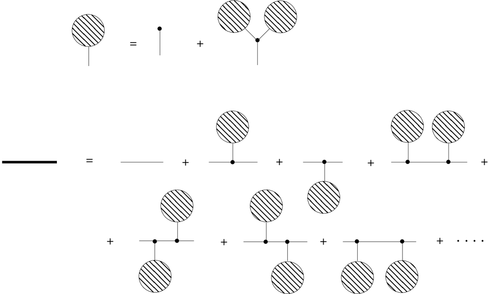
Figure 2: Top figure: the graphic equation defining the summation over all rooted trees. Bottom figure: The graphic equation for the dressed propagator which appears in Fig. 1 after summing over all tree-outgrows.

This formula captures the different ways one can take the scaling limit for the model given by $V_{0}(\phi)$. The tree sub-graphs shown in the left part of Fig. 1 and in the top part of Fig. 2 have the partition function $\alpha(\kappa)$ given in (10), and become critical for $\kappa^{2}\to 1/4$. The average number of vertices in a tree is

$$\langle n\rangle_{\kappa}=\frac{\kappa}{\alpha}\,\frac{d\alpha}{d\kappa}\sim\frac{1}{\sqrt{1-4\kappa^{2}}}.$$ (17)

Similarly, the average number of vertices $\langle n_{prop}\rangle_{\kappa}$ associated with trees attached to the dressed “propagator” shown in Fig. 2 diverges when $\kappa^{2}\to 1/4$. The partition function for the number of such vertices is $\beta(\kappa)$ defined in (12), and

$$\langle n_{prop}\rangle_{\kappa}=\frac{\kappa}{\beta}\,\frac{d\beta}{d\kappa}\sim\frac{1}{1-4\kappa^{2}}.$$ (18)

Thus the total average number of trees attached to a dressed propagator is proportional to $1/\sqrt{1-4\kappa^{2}}$. Since $\kappa\leq\kappa_{c}$ we conclude from eq. (8) that if we keep $g>0$ fixed when taking the scaling limit $\kappa\to\kappa_{c}$ the trees will not be critical since $\kappa_{c}^{2}<1/4$. Thus the trees can basically be ignored in the scaling limit $\kappa\to\kappa_{c}$. Eq. (16) captures this: for $g>0$ it tells us that

$$\frac{{\kappa_{{\rm dt}}}}{({\kappa_{{\rm dt}}})_{c}}=\frac{\kappa}{\kappa_{c}}\,\Big{(}1+O((\kappa_{c}-\kappa)^{2})\Big{)}.$$ (19)

The critical behavior is thus the standard one of DT and the graphs responsible for this are the standard $\phi^{3}$ graphs. In this scaling limit we write

$$\frac{\kappa}{\kappa_{c}}=1-a^{2}\Lambda+o(a^{2}),$$ (20)

where $\Lambda$ may be interpreted as the cosmological constant.

Clearly, to obtain a different scaling limit we have to scale $g$ to zero when $a\to 0$. The GCDT limit was obtained by the scaling $g=G\,a^{3}$, and using (9) we obtain from (16)

$$\frac{{\kappa_{{\rm dt}}}}{({\kappa_{{\rm dt}}})_{c}}=\frac{\kappa}{\kappa_{c}}\,\left(\frac{3G^{2/3}}{3G^{2/3}+2\Lambda}\right)^{3/4}.$$ (21)

This shows that ${\kappa_{{\rm dt}}}$ does not become critical as $\kappa\to\kappa_{c}$. Thus there is only a finite average number of vertices and links and faces in the skeleton graph. The critical behavior for $\kappa\to\kappa_{c}$ is entirely determined by the trees.

In order to obtain a new limit, let us consider the scaling

$$g=G_{\alpha}a^{\alpha},~{}~{}~{}~{}0<\alpha<3,$$ (22)

while maintaining (20), which states that we view the total number of vertices as proportional with the continuum area of the graph. With this scaling of $g$ we obtain from (9) and (16)

$$\frac{{\kappa_{{\rm dt}}}}{({\kappa_{{\rm dt}}})_{c}}=\left(1-\frac{\Lambda}{2G_{\alpha}^{2/3}}\,a^{2-2\alpha/3}+o(a^{2-2\alpha/3})\right).$$ (23)

By a scaling like (22) we thus obtain that both the trees and the skeleton graphs are critical. The average number of graph vertices per link in the skeleton graph is

$$\langle n_{prop}\rangle_{\kappa}\sim\frac{1}{1-4\kappa^{2}}\sim\frac{1}{a^{2\alpha/3}},$$ (24)

while the average number of skeleton vertices will be

$$\langle n_{skel}\rangle_{\kappa}\sim\frac{1}{a^{2-2\alpha/3}},$$ (25)

implying that the total number vertices in a typical graph scales as $a^{-2}$, in accordance with (20). Notice also that the average length of a skeleton link scales as $1/\sqrt{1-4\kappa^{2}}\sim a^{-\alpha/3}$.

In order to study the fractal properties of this ensemble of graphs one may calculated the so-called two-point function [4, 5], i.e. the partition function with two distinguished vertices separated by a given link distance $r$. It can be calculated using the methods in [10] or [4, 5]. For small $g$, $\kappa$ close to $\kappa_{c}$ and $r\gg g^{-1/3}$ one finds (up to numerical constants)

$$Z_{\mu}(r,g)\sim\Big{(}g^{2/3}\mu\Big{)}^{3/4}\;\frac{\cosh\Big{(}(g^{2/3}\mu)^{1/4}\,r\Big{)}}{\sinh^{3}\Big{(}(g^{2/3}\mu)^{1/4}\,r\Big{)}},~{}~{}~{}~{}\mu=\frac{\kappa_{c}-\kappa}{\kappa_{c}}.$$ (26)

Let us now take the scaling limit prescribed by eqs. (20) and (22). Insisting on keeping $G_{\alpha}$ and $\Lambda$ fixed and eliminating the scaling parameter $a$ in favor of $\mu$ leads to

$$Z_{\mu}(r)\sim(K\mu^{1/d_{H}})^{3}\,\frac{\cosh(K\mu^{1/d_{H}}r)}{\sinh^{3}(K\mu^{1/d_{H}}r)},~{}~{}~{}K=\Big{(}\frac{G}{\Lambda^{\alpha/2}}\Big{)}^{1/6},$$ (27)

which holds for $r\gg\mu^{-\alpha/6}$ and where

$$d_{H}=\frac{4}{1+\alpha/3}.$$ (28)

Since $(1-\mu)$ is a generating variable for the number $N$ of vertices in the graph, we find that the (canonical) two-point function $Z_{N}(r)$ for fixed $N$ is of the form ,

$$Z_{N}(r)\sim F(r/N^{1/d_{H}})\quad\text{for }r\gg N^{\alpha/6}$$ (29)

where $F(R)$ is some function that goes to zero fast for $R\gg 1$. In particular, this implies that the average distance $\langle r\rangle$ between arbitrary vertices is of the order $N^{1/d_{H}}$. For this reason one may call the exponent $d_{H}$ the “global” Hausdorff dimension [4, 5].

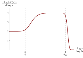
Figure 3: The scale-dependent Hausdorff dimension for $0<\alpha<3$.

The dimension $d_{H}$ should be contrasted with the “local” Hausdorff dimension $d_{h}$, which is associated with the growth $V(R)\sim R^{d_{h}}$ for small $R$ of the expected volume $V(R)$ of a disk as function of its radius $R$ within a fixed continuous geometry. In order to associate a well-defined Hausdorff dimension $d_{h}$ to our ensemble of graphs, one first has to specify how to scale the distance $r$ in the continuum limit. If one defines the continuum distance $R$ as $R=ra^{2/d_{H}}$ eq. (27) reduces to

$$Z_{\mu}(r)\sim\frac{\cosh(\Lambda^{1/4}G_{\alpha}^{1/6}R)}{\sinh^{3}(\Lambda^{1/4}G_{\alpha}^{1/6}R)},$$ (30)

which, up to the factor $G_{\alpha}^{1/6}$ is precisely the DT two-point function and therefore $d_{h}=4$. If, on the other hand, we scale $R=ra^{\alpha/3}$, the skeleton edges will maintain a finite length in the continuum, meaning that the local Hausdorff dimension is determined by that of the trees, i.e. $d_{h}=2$.

These observations can be summarized by looking at the “scale-dependent” Hausdorff dimension

$$d_{h}(N;r):=\frac{\mathrm{d}\log\langle N(r)\rangle}{\mathrm{d}\log(r)}$$ (31)

for a fixed large $N$, where $\langle N(r)\rangle$ is the expected number of vertices within graph distance $r$ from a randomly chosen vertex. A qualitative plot of $d_{h}(N;r)$ as function of $\log(r)/\log(N)$ for some $0<\alpha<3$ is shown in Fig. 3. The local Hausdorff dimensions, $d_{h}=2$ and $d_{h}=4$, appear as plateaus, while the global Hausdorff dimension corresponds to the scale at which $d_{h}(r)$ drops to zero.

3 Discussion

The partition function

$${\cal Z}=\int d\phi\;\mbox{e}^{-\frac{N}{g}\mathrm{tr}\,[-\kappa\phi+\frac{1}{2}\phi^{2}-\frac{\kappa}{3}\phi^{3}]}$$ (32)

generates a statistical ensemble of graphs of the kind shown in Fig. 1. The coupling constant $g$ in the action (4) can be viewed as the temperature $kT$ of this statistical system. Thus a scaling limit where $g>0$ corresponds to a finite temperature, and this finite temperature limit can be identified with the standard scaling limit of 2d Euclidean quantum gravity: i.e. the typical geometry of the ensemble is fractal with Hausdorff dimension $d_{h}=4$.

The scaling limit $g\to 0$ has certain analogues with the annealing, quenching and tempering of alloys and metals, in the sense that the precise way we take this zero temperature limit decides the smoothness of a typical geometry dominating at zero temperature. The parameter controlling this is the exponent $\alpha$ when writing $g=G_{\alpha}a^{\alpha}$, $0\leq\alpha\leq 3$, which tells us how “fast” we cool to zero temperature. The so-called global Hausdorff dimension $d_{H}$ of a typical graph in such an $\alpha$-ensemble is given by

$$d_{H}=\frac{4}{1+\alpha/3},$$ (33)

while, depending on the chosen scaling of the geodesic distance, the local Hausdorff dimension is either $d_{h}=4$ or $d_{h}=2$.

Here we have only considered the simplest situation, that of spherical (or disk) topology of the graphs and the associated geometries. It remains to be seen if there exists a complete perturbative expansion in topology and in number of boundaries for an arbitrary value of $\alpha$, as is the case in the two limits $\alpha=0$ and $\alpha=3$.

Acknowledgments

The authors acknowledge support from the ERC-Advance grant 291092, “Exploring the Quantum Universe” (EQU). JA acknowledges support of FNU, the Free Danish Research Council, from the grant “quantum gravity and the role of black holes”. In addition JA was supported in part by Perimeter Institute of Theoretical Physics. Research at Perimeter Institute is supported by the Government of Canada through Industry Canada and by the Province of Ontario through the Ministry of Economic Development & Innovation.

References

- [1] J. Ambjørn, J. Jurkiewicz and Yu.M. Makeenko, Phys. Lett. B 251 (1990) 517-524.
- [2] H. Kawai, N. Kawamoto, T. Mogami and Y. Watabiki, Phys. Lett. B 306 (1993) 19-26 [hep-th/9302133].
- [3] Y. Watabiki, Prog. Theor. Phys. Suppl. 114 (1993) 1-17.
- [4] J. Ambjørn and Y. Watabiki: Nucl. Phys. B 445 (1995) 129-144 [hep-th/9501049].
- [5] J. Ambjørn, J. Jurkiewicz, Y. Watabiki, Nucl. Phys. B454 (1995) 313-342. [hep-lat/9507014].
-
[6]
J.-F. Markert and A. Mokkadem. Ann. Probab. 34 (2007) 2144-2202
J.-F. Le Gall. Invent. Math. 169 (2007) 621-670
G. Miermont, Acta Math. 210 (2013) 319-401
J.-F. Le Gall. Ann. Probab. 41 (2013) 2880-2960 -
[7]
J. Ambjørn, R. Loll, Y. Watabiki, W. Westra, S. Zohren,
Phys. Lett. B670 (2008) 224-230.
[arXiv:0810.2408 [hep-th]].
J. Ambjørn, R. Loll, Y. Watabiki, W. Westra, S. Zohren, JHEP 0805 (2008) 032. [arXiv:0802.0719 [hep-th]].
J. Ambjørn, R. Loll, W. Westra, S. Zohren, JHEP 0712 (2007) 017. [arXiv:0709.2784 [gr-qc]]. - [8] J. Ambjørn, R. Loll, Nucl. Phys. B536 (1998) 407-434. [hep-th/9805108].
- [9] J. Ambjørn, L. Glaser, Y. Sato and Y. Watabiki, Phys. Lett. B 722 (2013) 172 [arXiv:1302.6359 [hep-th]].
- [10] J. Ambjørn and T. G. Budd, J. Phys. A: Math. Theor. 46 (2013) 315201 [arXiv:1302.1763 [hep-th]].
- [11] É. Fusy and E. Guitter, arXiv:1403.3514 [math.CO].