Optimal investment with time-varying stochastic endowments
This paper considers a utility maximization and optimal asset allocation problem in the presence of a stochastic endowment that cannot be fully hedged through trading in the financial market. After studying continuity properties of the value function for general utility functions, we rely on the dynamic programming approach to solve the optimization problem for power utility investors including the empirically relevant and mathematically challenging case of relative risk aversion larger than one. For this, we argue that the value function is the unique viscosity solution of the Hamilton-Jacobi-Bellman (HJB) equation. The homogeneity of the value function is then used to reduce the HJB equation by one dimension, which allows us to prove that the value function is even a classical solution thereof. Using this, an optimal strategy is derived and its asymptotic behavior in the large wealth regime is discussed.
Keywords. Utility maximization; Hamilton-Jacobi-Bellman equation; stochastic endowment; viscosity solution. In the present paper, we analyze the utility maximization or optimal investment problem of an economic agent who receives stochastic endowments over a finite time period. We deal with an incomplete market setting as the endowment risk is not perfectly correlated with the traded assets in the market. A specific example to motivate our model would be an economic agent who receives random salaries during her working life and invests a fixed proportion of the salaries in financial assets, optimizing the utility of her wealth at the retirement age. Another example could be a pension fund which receives random contributions from the members of the pension fund and invests to generate cash flows. In fact, the original idea of the paper arises from the study of defined contribution (DC) pension plans. This kind of pension scheme has become very popular over the last years and is substituting defined benefit pension plans (see e.g. [7]). In all OECD countries, defined contribution (DC) plans have played an increasingly important role in the last decades, see also the discussion in [7] for further reasons for the transition from originally dominant defined benefit pension plans towards DC plans. In a DC plan, pension beneficiaries typically contribute a fraction of their salary to the fund. Salaries or wages of the pension beneficiaries, typically consisting of a fixed part and a performance-related part (depending often on the company-wide, departmental as well as individual success), can be considered random. Likewise, it is reasonable to consider contributions as being random due to unforeseen changes in wages or salary, unemployment or reduced working hours, which has for example been faced by many workers due to the COVID pandemic. However, a perfect correlation to the traded risky assets is obviously unrealistic. In other words, the salary/contribution risk is not fully hedgeable in the financial market. In a DC plan, the pension beneficiaries bear the entire investment risk. For instance, DC beneficiaries in the U.S. manage the investment risk by so-called “Individual Retirement Accounts”, or more frequently by making contributions to so-called 401(k) plans, see [9] and [6] for details on these plans. The stochastic optimization problem developed in this paper can be straightforwardly applied in this retirement saving problem.
The problem of maximizing the expected utility of an economic agent by investment and/or consumption dates back to [31] and [32] and is further studied e.g. in [12, 17, 19, 28], just to quote a few. Such problems have originally been solved using the dynamic programming approach which requires the assumption of Markovianity on the state process and leads to a Hamilton-Jacobi-Bellman (HJB) equation. In the literature, this approach is called primal approach. In the 1980s, researchers develop an alternative approach, the so called dual approach where the assumption of Markovian asset prices can be relaxed to solve the optimal investment problem. In a complete market setting the dual method has been studied e.g. in [10, 37] and in an incomplete market setting e.g. by [23] and [24].
In the present paper, we consider the optimal asset allocation problem on a finite time horizon for an investor receiving an exogenous stochastic endowment modeled as a time-inhomogeneous geometric Brownian motion. We follow the primal HJB approach and argue that, in the case of power utility and under suitable regularity assumptions on the market parameters, the value function is a classical solution of the HJB equation. To obtain these results, we use a viscosity solution approach combined with classical existence results on regular solutions for nonlinear parabolic partial differential equations. More precisely, we first argue that the value function is the unique continuous viscosity solution of the HJB equation. Using the fact that the value function is homogeneous, we reduce the dimension of the HJB equation by one and obtain a fully nonlinear second-order parabolic equation which is uniformly elliptic in the spatial variable. From this, we are able to argue that the value function is even a classical solution of the HJB equation.
Proceeding from there, we then construct an optimal trading strategy. Since we restrict to strategies taking values in a compact-convex set, we shall see that it is a priori not clear if the stochastic differential equation (SDE) for the wealth process under the candidate optimal strategy (given in feedback form through the maximizer of the Hamiltonian in the HJB equation) admits a strong solution due to a lack of global Lipschitz properties of the drift and diffusion coefficients of the SDE. We are therefore forced to follow a non-classical approach to the construction of an optimal strategy: We first argue that an optimal strategy exists and then show that it can be represented in feedback form. In particular, this implies that the optimal strategy is unique. Given the optimal strategy, we finally analyze its asymptotic properties for large wealth-to-endowment ratios. We find that, asymptotically, the optimal strategy converges to the famous Merton ratio, which is the optimal strategy in the absence of random endowments.
The idea of incorporating a stochastic endowment in the classical utility maximization problem is indeed not new. Both dual and primal approaches (sometimes combined with Backward Stochastic Differential Equation (BSDE) techniques) are adopted to solve this optimization problem. Most of the papers in this field restrict themselves however to the analytically more tractable case of exponential utility functions (among several others [15] and [26]). Some authors deal also with the problem of maximizing expected power utility of terminal wealth in the presence of exogenous endowments. In [13], the problem is solved via duality for a broad class of utility functions under the assumption that the random endowment is bounded. The existence and uniqueness of an optimal control are proven, but an explicit representation of the optimal strategy is subordinated to the decomposition of the elements of into a regular and a singular part, which is hard to characterize explicitly. The authors of [27] overcome the problem and relax the hypothesis of boundedness by introducing the number of random endowments as a new control variable. [33] aims to examine under which conditions on the market model and on the utility stochastic field the maximizer of the optimal consumption problem exists. In addition, [33] looks into the properties of the value function and the corresponding dual problem. [34] studies existence and uniqueness of optimal investment and consumption strategies in a general incomplete semimartingale setting and provides a dual characterization in terms of an optional strong supermartingale deflator and a decreasing process. [44] focuses on examining the stability of the utility maximization problem with random endowment, i.e. when there is model and/or preference misspecification for the optimal investment problem. [25] extends the approach of [26] to the case of power utility functions, based on the martingale optimality principle combined with BSDE methods. They reduce the problem to the solution of a fully-coupled forward-backward stochastic differential equation, which is still not easy to solve.
Most closely related to our paper are [5] and [17]. The setting of [5] is similar to ours and considers a utility maximization problem with stochastic income modelled by geometric Brownian motion. However, they find a near-optimal consumption and investment strategy which leads to a small wealth-equivalent loss compared to the unknown optimal strategy. In [17], the expected HARA utility from consumption is optimized over an infinite-time horizon and it yields an elliptic HJB equation, not depending on time. We adopt and extend their methods, developed in the elliptic case (infinite-time horizon), to the parabolic case (finite-time horizon). We further extend their model to a slightly broader class of random endowments, i.e., we allow for time-varying coefficients. Most importantly, while [17] deals exclusively with the case of relative risk aversion less than one, we additionally extend the model to the empirically more relevant case of power utilities with relative risk aversion larger than one111 Note that there exist many empirical and experimental studies estimating the relative risk aversion (RRA) coefficients of individual investors. Although the resulting RRA levels differ among cases, all the levels seem to be larger than 1. For example, [2] finds that 65% of their data shows a RRA above 3.76, 24% below 2 and 12% between 2 and 3.76. [14] describes 3, 4 and 5 as most reasonable estimates of RRA and [1] estimates 3.01 and 3.74 as interval bounds for the RRA.. Especially the extension to the latter class of utility functions poses significant mathematical challenges in the viscosity characterization of the value function. In fact, we are able to establish a strong comparison principle for the (unreduced) HJB equation which covers the large relative risk aversion case as well, which is often a significant challenge in utility maximization problems; see, e.g., [38, 4].
The key property which makes our model tractable enough to construct a classical solution of the HJB equation, and hence to construct an optimal trading strategy, is the homogeneity of the value function in the power utility case. Ultimately, as already observed in [17] in the infinite horizon optimal consumption problem, this property follows from the homogeneity of the utility function and the multiplicative dependence of the state processes on their initial values. We use the homogeneity of the value function to reduce the dimension of the state space by one, which is the key to establish the existence of a classical solution of the HJB equation. Note, however, that our reduced-form value function still depends on wealth through the wealth-to-endowment ratio, so even after the reduction our problem is fundamentally different to the setting in the classical work [42] on optimizing expected utility in the presence of unhedgeable risk.
Another advantage of our HJB approach is that it is highly amenable to numerical solutions and thus allows to investigate economic questions such as the qualitative behavior of the optimal strategy. We illustrate this by briefly comparing the optimal investment strategies of young and old (i.e. close to retirement) investors and by considering whether the widespread life cycle investment strategies following the principle “the older you are, the less risky you should invest” can be theoretically justified by our theory.
The remainder of the paper is organized as follows. Section 1 describes the model setup and particularly the endowment process. In Section 2, we introduce the optimization problem and study some of its basic properties such as well-posedness, continuity, concavity, and homogeneity. In Section 3 we restrict ourselves to power utility and study properties of the associated HJB equation. Here, we show that the value function is the unique viscosity solution of the HJB equation and prove that it is even a classical solution if the market parameters are sufficiently regular. In Section 4, we construct an optimal strategy in the regular case and analyze its asymptotic behavior as the wealth-to-endowment ratio approaches infinity. In Section 5, we apply numerical methods to illustrate concrete economical insights that can be gained. Finally, Section 6 concludes the paper.
1 The model
On a fixed filtered probability space satisfying the usual hypotheses, consider a financial market consisting of a riskless and a risky asset. From now on let be a fixed finite time point. Let and denote respectively the savings account and the risky asset. We assume that the two assets follow a Black-Scholes model:
where and is a Brownian motion on our filtered probability space.
The endowment process is assumed to have stochastic dynamics driven by another Brownian motion defined on the same probability space, which is assumed to be correlated with with a correlation coefficient222We exclude the perfect correlation cases and . In these extreme cases, both the risky asset and the random income are fully driven by . The optimization problem becomes simpler and differs from what we will present in the remaining text. For instance, in a retirement context, [18] study the optimal consumption and retirement problem with stochastic labor income, where the labor income is perfectly correlated with the financial market risk. In other words, we assume that there is another Brownian motion independent of such that , which leads to the random endowment process given by
where and , are deterministic continuous functions.
Remark 1.1.
Time-homogeneous geometric Brownian motions are sometimes chosen in the literature to model a stochastic income (see [39]). Thinking of the example of a DC pension scheme, we can interpret the process as a diffusion income, or rather a proportion of it possibly changing over time, which is paid continuously into the pension fund. From an analytical point of view, the fundamental feature of this family of random endowments is that, in the power utility case, the value function of the optimization problem turns out to be homogeneous in the spatial variables. This is the crucial property to achieve a reduction in the dimension of the problem. Allowing for deterministic time varying drift and volatility does not substantially change the following mathematical analysis. It seems realistic that both drift and volatility of the income are somewhat higher at the beginning of a career than close to retirement.
We assume that an agent with an initial wealth invests at any time a proportion of the wealth in the stock and in the risk-free asset with interest rate . In addition, the random income is paid continuously to the account at rate . The wealth process corresponding to the strategy , denoted by , is assumed to have the following dynamics:
Defining , this can be written as
| (1.1) |
This definition reflects the fact that the only additional cash injections are due to the continuous payments at rate .
Note that in our set-up a strategy encodes the fraction of the overall wealth invested in the risky asset. We assume that is a progressively measurable process taking values in a compact-convex set for real numbers . This includes the case of short-selling of the risky asset and borrowing of cash being restricted. We write for the set of all such trading strategies. To compare and discuss optimal trading in the presence and the absence of random endowments, we subsequently assume , where denotes the Merton fraction
It is a classical result that is the optimal strategy in the absence of random endowments, i.e. in case of , and power utility with being the relative risk aversion. Let us highlight that our compactness assumption does not imply that the money invested in the risky asset or the cash position is bounded. Instead it means that there is a relative bound on the extent to which short-selling of the risky asset and taking credit on the bank account is allowed. As an example, choosing amounts to assuming that short-selling of the risky asset and borrowing of cash are prohibited. Mathematically, the compactness assumption makes the study of the value function of the optimal investment problem significantly easier than in the unrestricted case. In fact, we shall make ample use of this assumption in our results in Section 2 and in the viscosity characterization in Section 3; see also the discussion before Theorem 3.4. In contrast, this trading constraint leads to significant challenges in the construction of an optimal strategy. In fact, even though we are able to show that the value function is a classical solution of the HJB equation and obtain a candidate optimal strategy in feedback form, it is unclear if the wealth process associated with the candidate optimal strategy exists; see the discussion in the beginning of Section 4 for details. We overcome this issue by first establishing an abstract existence result for optimal strategies and subsequently verifying that any optimal strategy coincides with our candidate optimal control.
Remark 1.2.
Evidently, as is compact, any is bounded. In particular, this ensures the existence and uniqueness of a solution for Equation (1.1).
Remark 1.3.
In the definition of admissibility, one usually has to ensure that the wealth process never becomes negative. Under our assumptions, the wealth process stays positive without any extra requirement on the admissible strategies. This can be seen from the fact that the explicit solution of (1.1) is given by
where is a stochastic exponential factor given as
2 The optimization problem: statement and properties
Recall that the Brownian motion represents the uncertainty in the income, which is supposed not to be traded in the market. This makes the market incomplete and we are hence facing the problem of maximizing expected utility of an individual in an incomplete market. More precisely, we are looking for an optimal investment strategy such that
where is a utility function which is twice continuously differentiable, increasing, concave, and satisfies the Inada conditions and .
Later on, we will restrict to the special case of being a constant relative risk aversion (CRRA) power utility function, i.e. for a risk aversion parameter , we shall assume that with
The power utility function is abundantly used in both theoretical and empirical research because of its analytical tractability. Further, both empirical and experimental studies (e.g. [2]) typically show that individuals demonstrate decreasing absolute risk aversion, and power utility falls into this category. In addition, the long-run behavior of the economy suggests that the risk aversion over long horizons, like for retirement decisions, does not strongly depend on wealth, see [8].
The agent is assumed to maximize expected utility of terminal wealth at the final time , and thus the value function of the utility maximization problem is given by333A priori, it is of course not evident that is finite or even well-defined. We shall, however, see in Proposition 2.2 below that the positive part of is integrable with a bound not depending on the trading strategy , in which case is well-defined as an -valued function.
| (2.1) |
where . In the definition of the value function, the state process is taken to be the pair and the notation and is used for the wealth and endowment process started at time in and , respectively.
2.1 A priori estimates, local boundedness, and continuity
We first provide simple sufficient conditions under which the value function is finite and continuous. A key ingredient is the following collection of a priori estimates on the state processes.
Lemma 2.1 (A priori estimates).
Let . Then there exist such that
| (2.2) | ||||||
| (2.3) | ||||||
| (2.4) |
Moreover, there exists a constant such that
| (2.5) |
for all .
Proof.
The estimate (2.5) follows from a direct application of Proposition 3.22 in [35] (applying Eq. (3.78) with , , and arbitrarily in the notation of [35]). To obtain (2.2), we first observe that an application of Itô’s lemma shows that the process satisfies the (linear) Lipschitz SDE
Classical a priori estimates for solutions of Lipschitz SDEs such as Corollary 2.10 in [30] applied to hence imply the existence of a constant such that
Turning to (2.3), we use that and to estimate
| (2.6) |
where, again by Itô’s lemma, solves the (linear) Lipschitz SDE
As before, we conclude that there exists a constant (independent of as the Lipschitz constant in the SDE for can be chosen independent of since the set is bounded) such that
and hence (2.3) is obtained. Finally, regarding (2.4), we note that
where we have to use Jensen’s inequality in the last step if . Applying again the a priori estimate for Lipschitz SDEs yields the existence of independet of such that
which implies (2.4) with . ∎
The a priori estimates can be used to provide simple sufficient conditions under which the value function is finite and is bounded uniformly from below for all admissible strategies. As usual we define the positive and negative part of a function and . Moreover, we remark that the Inada condition at infinity, i.e. , implies that there exist constants and such that
| (2.7) |
E.g., in the case of power utility , this estimate holds for if and if .
Proposition 2.2 (Local boundedness).
-
(i)
Let such that (2.7) holds. Then there exists a constant such that
-
(ii)
Suppose that there exist constants and such that . Then there exists a constant such that
In particular, in this situation, the value function is locally bounded, i.e. there exists a constant such that
Proof.
Note that for power utility functions with the assumption of part (ii) of the proposition is satisfied with and that for the positive part and for the negative part vanishes. The logarithmic utility is an example of a common utility function for which the result applies and for which neither the positive nor negative part is zero.
In the next step, we derive continuity properties of the value function. This is done under the same assumptions as in the previous proposition together with a suitable growth condition on the derivative of the utility function.
Proposition 2.3 (Continuity).
Suppose that there exist constants and as well as constants and such that
| (2.8) |
Then we can find such that
for all . In particular, is locally Lipschitz continuous in and locally -Hölder continuous in .
Proof.
Let and assume, without loss of generality, . For , we let be an -optimal strategy in that
Note that exists since . Moreover, Proposition 2.2 guarantees that
With this, using the concavity of , the growth assumption on , and finally Hölder’s inequality, we obtain the estimate
| (2.9) |
Applying the a priori estimate (2.3) now shows that
| (2.10) |
and the a priori estimate (2.5) yields
| (2.11) |
where we have used the subadditivity of the square root function for the last step. Note that neither of the constants depends on the strategy and hence does not depend on either. Now plugging (2.10) and (2.11) into (2.9) leads to
The result follows as is chosen arbitrarily and does not depend on . ∎
Note that the power utility function satisfies the assumptions set forth in the previous proposition with and . For later reference, we gather these results in a corollary.
Corollary 2.4 (Power utility).
Suppose that is a power utility function, i.e. for with . Then there exists a constant such that
| (2.12) |
where and . Moreoever, is continuous and satisfies
for all for a constant .
2.2 Further properties of the value function
Before turning to the HJB equation associated with the optimization problem, we first study some further properties of the value function. In particular, we shall see that is concave and monotone in the spatial variables. Moreover, in the special case of power utility, we show that is homogeneous of degree .
Proposition 2.5 (Monotonicity and concavity).
is increasing and jointly concave in the spatial variables. In particular, for every fixed , the mapping is locally Lipschitz continuous on the interior of its effective domain .
We note that, in Proposition 2.3, we have established a stronger continuity result. However, for this we have to assume (2.8), whereas Proposition 2.5 is valid without additional assumptions.
Proof of Prop. 2.5.
The proof works along standard lines (cf., e.g., Section 3.6.1 in [36]). Note that continuity follows immediately from concavity, as every concave function is locally Lipschitz continuous in the interior of its effective domain.
Step 1: Monotonicity. Let us fix , with and , and a strategy . Since the endowment process is a geometric Brownian motion we see that
and from the explicit representation of the wealth process we find that
Since was chosen arbitrarily and the utility function is monotone, this shows that
i.e. is monotone in both its second and third argument.
Step 2: Concavity. Let us again fix and . Let moreover , choose , and define
Moreover, with , , we define
As is a convex combination of and , it follows that is -valued and hence is admissible. Let us show that is the wealth process corresponding to . For this, observe that
implying that
and hence uniqueness of solutions of linear SDEs implies that , i.e. is the wealth process corresponding to started in . Using the concavity of the utility function, we get
but since are chosen arbitrary, taking the supremum on the right hand side, we arrive at
We conclude this section by showing that, in the power utility case , the value function is homogeneous of degree in the spatial variables.
Lemma 2.6 (Homogeneity).
Suppose that with , . Then the value function is homogeneous of degree in the spatial variables, i.e.
As a consequence, can be represented in separable form as
where
| (2.13) |
Proof.
The separable representation of follows immediately from homogeneity with since
To see that is homogeneous, fix , , and . Since we find that
But then must be homogeneous of degree since
3 The Hamilton-Jacobi-Bellman equation
Henceforth, we restrict our attention to power utility, i.e. . Applying well-known principles of stochastic control, see e.g. Chapter 3 in [36], we can write down the HJB equation for the value function of our control problem:
| (3.1) | ||||||
where the linear differential operator is defined through
Here, and in the following, we denote partial derivatives by subscripts and often omit the argument of functions in the equations. The aim of this section is to characterize the value function as the unique viscosity solution of the HJB equation. Moreover, we show that is even a classical solution provided that and are continuously differentiable.
3.1 A family of supersolutions
Before linking the value function to the HJB equation, let us first study the existence of classical supersolutions of the HJB equation. These play a crucial role for our subsequent analysis and serve, in particular, as abstract boundary/growth conditions for the HJB equation.
We begin by defining two constants
as well as
With this, we introduce a parametric family of functions
for with , , and . We assume that takes the form
for all , where the function is given as the unique solution of the ordinary differential equation
Observe that unless and . In any case, is nonnegative and hence, in particular, well-defined. We proceed to show that is a classical supersolution of the HJB equation.
Proposition 3.1 (Classical supersolution).
For any choice of with , , and , the function is a supersolution of the HJB equation, i.e.
Moreover, it is a strict supersolution if .
Proof.
We decompose as , where
By linearity of the operator , it follows that
Hence, in order to conclude, it suffices to show that and are supersolutions, and is a strict supersolution if .
Step 1: is a (strict) supersolution. If , then and it is thus a solution of the HJB equation. Let us hence assume that and prove that, in this case, is a strict supersolution. Setting , the partial derivatives of are given by
Plugging these derivatives into the HJB equation and rearranging terms yields
By the choice of , the terms inside the brackets are nonnegative and hence
i.e. is a strict supersolution of the HJB equation.
Step 2: is a supersolution. Writing and using the ordinary differential equation for , the partial derivatives of are given by
Plugging these derivatives into the HJB equation and rearranging terms yields
Instead of maximizing over we can maximize over all of , making the last expression smaller in doing so. The maximizer in the supremum is given by
Plugging this into the above equation and rearranging terms again then yields
where the nonnegativity follows from the choice of . ∎
With the existence of classical supersolutions, we can derive tight bounds on the value function.
Proposition 3.2 (Tight bounds on ).
The value function satisfies
Proof.
Step 1: We first prove the lower bound. For this, consider the constant strategy and recall that . But then
The last expectation can be computed explicitly and is given by
Step 2: To prove the upper bound, let as well as and write and . For fixed, set and denote by , , a localizing sequence of the local martingale
Applying Itô’s lemma to and using the fact that is a supersolution of the HJB equation, it follows that
As , we see that is lower bounded. Hence we may apply Fatou’s lemma to arrive at
Since was chosen arbitrarily, this implies that and hence
Remark 3.3.
Another way to prove estimates on is to use financial arguments as follows:
-
•
The lower bound corresponds to the value function of the problem without random endowments and can therefore be improved when random endowments are present;
-
•
An alternative upper bound could be found by comparing the problem to the one of an artificial market model where the endowment can also be traded.
3.2 Viscosity characterization of the value function
The next step is to show that the value function is the unique viscosity solution of the HJB equation. We refer to [11] for the definition of (and all important results on) viscosity solutions of second order PDEs. While the fact that is a viscosity solution of the HJB equation is standard, the uniqueness result poses significant challenges in the case of as the value function tends to near the boundary of the state space. To handle this issue, we require a sufficiently strong comparison principle for the HJB equation.
Before turning to the comparison principle, let us record that the Hamiltonian
given by
for , and with
is both finite everywhere and continuous. Note that, for this, it is crucial that is compact, since otherwise the Hamiltonian may diverge at some points of its domain, hence making the following viscosity characterization more involved. We also note that if is a sufficiently smooth function, it holds that
where and denote, respectively, the gradient and the Hessian of with respect to the spatial variables . One important consequence of the continuity of is that, by Lemma V.6.1 in [22], we are allowed to apply the parabolic version of Ishii’s lemma; see Theorem V.6.1 in [22].
Theorem 3.4 (Comparison principle).
Let such that is an upper semi-continuous viscosity subsolution and is a lower semi-continuous viscosity supersolution of the HJB equation with
| (3.2) |
Suppose furthermore that on . Then
Proof.
Step 1: Setup of the proof and definitions. We argue by contradiction and suppose that there exists such that
| (3.3) |
For and , we introduce a function given by
Here, for some with . We recall that is a strict classical supersolution of the HJB equation and takes the form
where is strictly positive on . Finally, we define a function by
and we shall subsequently assume that is sufficiently small to guarantee that
which is possible by (3.3).
Step 2: Maximizers of . For each , we define
Let us first observe that for all as, clearly, is decreasing in (implying ) and
Moreover, using (3.2), we note that for each and we have
Since and , it follows that
Similarly, we see that
In particular, as is upper semicontinuous, we find that
and, as and , any maximizing sequence for any , , is contained in . Moreover, upper semicontinuity of implies that we find such that
Step 3: Convergence of maximizers. As is compact and for all , after passing to a subsequence if necessary, it follows that
for some . Moreover, we note that implies
| (3.4) |
For the finiteness of the last expression, we have used that and are upper semicontinuous and finite-valued on the compact set . Since (3.4) is finite and does not depend on , it follows that . From this, using that and then upper semicontinuity of both and and continuity of , it follows that
In particular, all inequalities must actually be equalities and the can be replaced by a proper limit. We have therefore argued that
as well as
Step 4: Application of Ishii’s lemma. Let us show that is not located on the boundary of the state space. As is a compact subset of and , we cannot have nor . Moreover, if , we use and the assumption that on to arrive at the contradiction
Thus, as , it follows that for all large enough and hence without loss of generality for all . We can therefore apply Theorem V.6.1 of [22] (Ishii’s lemma) to obtain the existence of and symmetric such that and
| (3.5) |
and such that444Here, and denote the closures of the second-order parabolic super- and subjets of a function at , respectively.
where
Step 5: The contradiction. As and are viscosity sub- and supersolutions, it follows that
Using the elementary inequality
it follows that
| (3.6) | ||||
Using (3.5), a standard estimate shows that
But then this and
allows us to continue to estimate (3.6) as follows:
where
Sending and using that is a strict supersolution of the HJB equation therefore yields
which is the desired contradiction and hence concludes this proof. ∎
Remark 3.5.
The main technical challenge in extending the results in [17] to the case of risk aversion larger than one (i.e. ) lies in the comparison principle. Indeed, for such values of , the utility function explodes as , which requires very precise control of the viscosity sub-/supersolutions near that part of the boundary to establish a comparison principle. In our situation, this is achieved by Propostion 3.2, which allows us to pin down the behaviour of the value function near .
With this comparison principle at hand, the stochastic Perron’s method [3] immediately implies that the value function is the unique continuous viscosity solution of the HJB equation.
Corollary 3.6 (Viscosity characterization).
The value function is the unique viscosity solution of the HJB equation (3.1) in the class of continuous functions satisfying the terminal condition
and the growth condition
3.3 Regularity of the value function
We now give sufficient conditions which guarantee that the value function is even a classical solution of the HJB equation. Related but different results can be found in [21] and [20]. The main obstacle to establishing regularity of the value function is the lack of uniform ellipticity of the HJB equation. However, the homotheticity property allows us to consider the transformation
| (3.7) |
where and . It turns out that solves a reduced-form HJB equation of the form
which is uniformly elliptic and admits a classical solution provided that and are continuously differentiable. Moreover, observe that by passing to we have reduced the dimension of the state space by one, which is advantageous for numerical computations.
Theorem 3.7 (Regularity).
Assume that and are continuously differentiable. Then . In particular, is a classical solution of the HJB equation.
Proof.
Step 1: The transformed HJB equation. Let us consider the equation
| (3.8) |
where
are given by
for , , , and where the parameter is chosen such that
| (3.9) |
Formally, Equation (3.8) arises if we consider the transformation
Now fix . Then we claim that Equation (3.8) admits a solution with satisfying the boundary and terminal conditions
| (3.10) |
Once this is established, we can define a continuous function
where denotes the closure of the set
Observe that, by the terminal/boundary condition (3.10) and the homogeneity of , we have
whenever or . Moreover, since solves (3.8) on , a straightforward calculation shows that solves the original HJB equation, i.e.
But then also satisfies this equation in the sense of viscosity solutions and hence on by the uniqueness result Theorem V.8.1 in [22]. In particular, we find that for each and we conclude by sending .
Step 2: We are left with showing that Equation (3.8) admits a classical solution on satisfying the boundary/terminal condition (3.10). For this, it is sufficient to verify the conditions in Theorem A.8 in [21]; see also Theorem 3 in Section 6.4 of [29] for the original result.
-
(i)
For every , it is clear that and are continuously differentiable and for each pair the function is twice continuously differentiable. Indeed, the non-zero derivatives are given by
From this, we also see that as well as all second-order derivatives of with respect to and are bounded on
-
(ii)
is uniformly elliptic on , i.e.
-
(iii)
For all , it holds that
Similarly, setting
it follows that
where is the continuous function given by
- (iv)
Under conditions (i) to (iv), Theorem 3 in Section 6.4 of [29] is applicable. This yields the existence of and the proof is complete. ∎
4 The optimal strategy and its asymptotic behavior
In this section, we construct an optimal strategy and study its properties as the ratio of wealth to endowment becomes large.
4.1 Existence and characterization of the optimal strategy
A candidate optimal strategy is readily found by computing the maximizer in the HJB equation. Indeed, a straightforward calculation shows that the unique maximizer of the Hamiltonian is given by
| (4.1) |
For any initial configuration , a candidate optimal strategy is defined on by555The strategy should of course be extended to an -valued process on . Note, however, that the function may not be well defined for . An argument as in Remark 3.1 (iv) in [40] shows that can without loss of generality be taken independent of , e.g. equal to a constant value.
where and is the solution of
| (4.2) |
We note, however, that is is unclear if the drift and diffusion coefficients
satisfy the necessary regularity to ensure the existence of a strong solution of (4.2). We therefore follow a different route: We first argue that for each initial configuration , an optimal strategy exists and then show that it can be represented in feedback form via the function . This somewhat unusual route is an artifact of our assumption of being compact. In fact, we expect that allowing trading strategies to take values in the entire real line makes it possible to use similar arguments as in [17] to construct the optimal strategy in a more classical way.
Proposition 4.1 (Existence of optimizers).
Let . Then there exists an optimal trading strategy , i.e.
Proof.
We employ a classical Komlos-type argument and show that suitable forward-convex combinations of a maximizing sequence for converge to an optimal strategy. Denote by such a maximizing sequence for , i.e. a sequence of admissible trading strategies with
For each , let us denote by the wealth invested in the stock under the strategy . We may extend to a process defined on by setting for all . Now observe that, by uniform boundedness of and the a priori estimate (2.4) in Lemma 2.1, it holds that
i.e. the sequence is bounded in the Hilbert space of progressively measurable and square-integrable processes. We can therefore apply Theorem 15.1.2 in [16] to find and a sequence with such that
Next, for each , let us introduce processes and with and given as the unique solution of
with on . Observe that is the wealth process corresponding to the trading strategy . Moreover, since , there exist , indices and convex weights such that . With this, we see that
from which we conclude by uniqueness of solutions of linear SDEs. But then
i.e. is a (dynamic) convex combination of and therefore -valued and admissible. Next, consider the wealth process given by
with on and observe that, using the dynamics of and , Jensen’s inequality, and the Itô isometry, there exists a constant such that
Gronwall’s inequality therefore yields
Setting , using the convergence of to , it follows that is -valued almost everywhere (hence without loss of generality everywhere after possibly redefining on a nullset) and hence admissible. Clearly, is the wealth process corresponding to . Moreover, since , it follows from Lemma 2.1 that is bounded in the space of square-integrable random variables and thus uniformly integrable. With this and using the concavity of , we hence conclude that
Next, let us proceed to show that any optimal strategy must necessarily be given in feedback form via the function defined in (4.1).
Theorem 4.2 (Optimal strategy in feedback form).
Fix , let be an arbitrary strategy, and suppose that . Then is optimal if and only if
| (4.3) |
where and .
Proof.
Step 1: Suppose that is an arbitrary strategy satisfying (4.3). Using that solves the HJB equation and is a pointwise maximizer of the supremum in the HJB equation, an application of Itô’s formula shows that
for all , i.e. is a local martingale. But since by (2.12) and Lemma 2.1
| (4.4) |
it follows that is an honest martingale and hence
i.e. is optimal.
Step 2: Suppose that is optimal, i.e.
| (4.5) |
An application of Itô’s formula and the fact that satisfies the HJB equation implies
| (4.6) |
for all . But as (4.4) is also valid in this situation, it follows that is a super-martingale and thus by (4.5) an honest martingale. Thus we must have equality in (4.6), i.e.
-almost everywhere on . Now the supremum on the right hand side has a unique maximizer given by the function and thus
and the proof is complete. ∎
4.2 Asymptotic behavior of the optimal strategy
In this section, we examine the asymptotic behavior of the value function and the optimal policy as the initial capital converges to infinity. We will see that for this model a sort of “turnpike property” holds (see e.g. [43]) in the sense that for (more precisely, as becomes large) the optimal policy approaches the Merton fraction of investing a constant proportion of wealth in the risky asset.
To make this statement precise, we subsequently write
whenever . Our aim in this section is hence to show that for all , where is the feedback function defined in (4.1). To prove this, we first recall the reduced value function defined in Lemma 2.6 and observe that
From this, it follows that can be rewritten as
| (4.7) | ||||
Theorem 4.3 (Asymptotics for the optimal strategy).
For any , we have
from which it follows that
Proof.
The statements on the asymptotic behavior of and its derivatives follow from the bounds on derived in Proposition 3.2. Indeed, the bounds on and homogeneity of imply that
From this and using monotonicity and concavity of all functions involved, we see right away that
But then
and it follows that
Since , we see that and the proof is complete. ∎
5 Numerical illustration
The strength of our approach is that we obtain a formula for the optimal strategy that is explicit in terms of the solution of the boundary value problem for the value function which in turn is highly amenable to numerical methods (for the plots shown in this section we implemented the finite difference methods of [41] in Matlab). This allows one to consider questions of high economic relevance. Below we briefly look at two of them, viz. the optimal equity holdings of young and old investors in their pension fund and later on whether the common wisdom that “the closer one is to retirement the lower the equity holdings should be” is indeed universally true. Throughout this section we take constant over time.
We now consider the optimal equity holdings as a function of time for an old and a young investor. We distinguish between the two investors by choosing a different initial value of the ratio between current wealth and income and a different investment horizon . A higher means a higher initial capital compared to the initial contribution. Note that the initial optimal investment strategy therefore always depends on the ratio of wealth over income. The young investor still needs to work for another 30 years until retirement and starts with a lower initial , while the old investor only needs to work for another 10 years and has an initial . The resulting optimal equity holdings are plotted in Figures 1 and 2 respectively. To gain a better intuition, Merton’s constant-mix portfolios are provided in the two graphics as well.
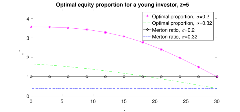
Here z=5, T=30 years, and , , , , , .
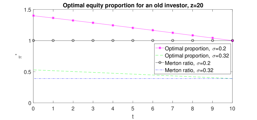
Here z=20, T=10 years, and , , , , , .
Comparing the solid curves in these two graphics, we observe the following: a) while Merton’s portfolio is a constant-mix one, which does not depend on time, the equity holdings resulting from random endowments are decreasing in time, demonstrating a so-called glide path. The closer the individual investors move to retirement, the less will be invested in the risky asset. b) Young investors have a longer time to work and have not had much time to accumulate wealth. The ability to work (human capital) is therefore their largest asset. Older investors have already converted most of their human capital to financial capital. In this sense, young investors can borrow from their future income to invest more in the risky asset, which leads to a substantially higher equity holding of the young investor. c) A higher volatility (keeping the drift fixed) makes the equity investment less interesting, which subsequently lowers the optimal equity holding.
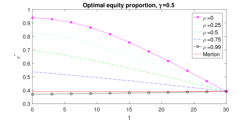
Parameters: years, , , , , , , .
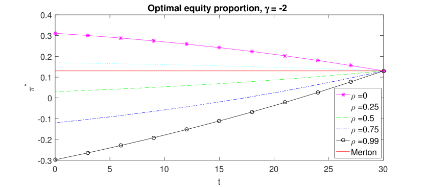
Parameters: years, , , , , , , .
In the above examples the common wisdom “the closer you are to retirement the less risky you should invest”, which is also behind many products sold to small private investors, seems to be true and our intuitive explanation is that a young investor borrows from her future income enabling her to go more risky. It is realistic that the income and the stock market are correlated, in most cases (except for e.g. liquidators) positively. This implies that future income changes can at least be partially hedged by investing in the stock market. In the case of a positive correlation this should imply that a risk averse investor should go short in the stock market to hedge her income. This effect should be more pronounced the more risk averse an investor is. Figures 3 and 4 depicting the optimal equity proportions for different values of as a function of time for and the more risk averse show that our model can reproduce these effects. The higher the correlation is, the lower (ceteris paribus) is the investment in the stock market in order to also hedge the future income changes. Note that for we have also taken a higher which makes an investment in the stock market more attractive. So for the same as in Figure 3 the optimal equity proportions held would be even lower. Interestingly, it turns out that the hedging effect can even be dominant implying that the closer one is to the higher is the optimal investment in the risky asset. This clearly shows that the mentioned common wisdom is far from being universally true: the more risk averse investors are, the less often it is true.
To characterize exactly when we have an optimal equity proportion above or below the Merton ratio seems to be a very challenging question. What we can establish is the following.
Proposition 5.1.
Assume that is constant over time and . If , then for the correlation of the Brownian motions being equal to
| (5.1) |
the corresponding optimal strategy is constant and coincides with the Merton ratio, namely
Proof.
We look for a sufficient condition on the correlation such that the optimal policy in (4.7) coincides with the Merton ratio. Define, for ,
Suppressing the arguments of , we now look for a such that
Rearranging the terms, this holds if and only if
Clearly, this equation is satisfied for . The fact that is strictly positive follows from Equation (5.1) since . Moreover, is a correlation coefficient thanks to the assumptions on the parameters. ∎
Combining this with our numerical results and assuming that lies in the interior of , it seems reasonable to conjecture that:
-
•
if , then for all ,
-
•
if , then for all .
This would also imply that for a sufficiently small relative risk aversion parameter (that is, sufficiently large), all values of the correlation should yield optimal strategies lying above the Merton ratio. In the set-up of Figure 3, the critical value is and for the parameter constellation of Figure 4.
6 Conclusion
We consider an optimal asset allocation problem in an incomplete market, where exogenous stochastic endowments flow continuously into the portfolio according to a time-inhomogeneous geometric Brownian motion. We analyze the viscosity solution of the HJB PDE, reduce its dimension, and prove that the optimal strategy can be recovered from the optimal policy of a reduced problem.
We are also able to describe the asymptotic behavior of the value function, and the strategy when the initial wealth goes to infinity. We illustrate that our results open the door for precise numerical studies and briefly explain some economic insights to be gained.
Acknowledgements
The authors thank the editors as well as the anonymous referees for their insightful and constructive comments which improved the paper significantly. They are very grateful to Nils Sørensen for preparing the plots included in this paper. Carla Mereu gratefully acknowledges financial support from the Graduiertenkolleg 1100 at Ulm University, funded by the DFG (Deutsche Forschungsgemeinschaft).
References
- [1] S. A. Azar, Bounds to the coefficient of relative risk aversion, Banking and Finance Letters, 2 (2010), pp. 391–398.
- [2] R. B. Barsky, F. T. Juster, M. S. Kimball, and M. D. Shapiro, Preference parameters and behavioral heterogeneity: An experimental approach in the health and retirement study, The Quarterly Journal of Economics, 112 (1997), pp. 537–579.
- [3] E. Bayraktar and M. Sîrbu, Stochastic Perron’s method for Hamilton-Jacobi-Bellman equations, SIAM Journal on Control and Optimization, 51 (2013), pp. 4274–4294.
- [4] C. Belak, O. Menkens, and J. Sass, On the uniqueness of unbounded viscosity solutions arising in an optimal terminal wealth problem with transaction costs, SIAM Journal on Control and Optimization, 53 (2015), pp. 2878–2897.
- [5] B. Bick, H. Kraft, and C. Munk, Solving constrained consumption-investment problems by simulation of artificial market strategies, Management Science, 59 (2013), pp. 483–503.
- [6] F. Bosserhoff, A. Chen, N. Sørensen, and M. Stadje, On the investment strategies in occupational pension plans, forthcoming in Quantitative Finance, (2021).
- [7] D. Broeders and A. Chen, Pension regulation and the market value of pension liabilities: A contingent claims analysis using parisian options, Journal of Banking & Finance, 34 (2010), pp. 1201–1214.
- [8] J. Y. Campbell and L. M. Viceira, Strategic asset allocation: portfolio choice for long-term investors, Oxford University Press, 2002.
- [9] C. Copeland, Target-date fund use in 401 (k) plans and the persistence of their use, 2007-2009, EBRI Issue Brief, (2011).
- [10] J. C. Cox and C.-F. Huang, Optimal consumption and portfolio choices when asset prices follow a diffusion process, Journal of Economic Theory, 49 (1989), pp. 33–83.
- [11] M. G. Crandall, H. Ishii, and P.-L. Lions, User’s guide to viscosity solutions of second order partial differential equations, Bulletin of the American Mathematical Society, 27 (1992), pp. 1–67.
- [12] D. Cuoco, Optimal consumption and equilibrium prices with portfolio constraints and stochastic income, Journal of Economic Theory, 72 (1997), pp. 33–73.
- [13] J. Cvitanić, W. Schachermayer, and H. Wang, Utility maximization in incomplete markets with random endowment, Finance and Stochastics, 5 (2001), pp. 259–272.
- [14] J. B. Davies, Uncertain lifetime, consumption, and dissaving in retirement, Journal of Political Economy, 89 (1981), pp. 561–577.
- [15] M. H. Davis, Optimal hedging with basis risk, in From stochastic calculus to mathematical finance, Y. Kabanov, R. Liptser, and J. Stoyanov, eds., Springer, 2006, pp. 169–187.
- [16] F. Delbaen and W. Schachermayer, The Mathematics of Arbitrage, Springer Finance, Springer-Verlag, Berlin, 2006.
- [17] D. Duffie, W. Fleming, H. M. Soner, and T. Zariphopoulou, Hedging in incomplete markets with HARA utility, Journal of Economic Dynamics and Control, 21 (1997), pp. 753–782.
- [18] P. H. Dybvig and H. Liu, Lifetime consumption and investment: retirement and constrained borrowing, Journal of Economic Theory, 145 (2010), pp. 885–907.
- [19] N. El Karoui and M. Jeanblanc-Picqué, Optimization of consumption with labor income, Finance and Stochastics, 2 (1998), pp. 409–440.
- [20] S. Federico, P. Gassiat, and F. Gozzi, Utility maximization with current utility on the wealth: regularity of solutions to the HJB equation, Finance and Stochastics, 19 (2015), pp. 415–448.
- [21] , Impact of time illiquidity in a mixed market without full observation, Mathematical Finance, 27 (2017), pp. 401–437.
- [22] W. H. Fleming and H. M. Soner, Controlled Markov Processes and Viscosity Solutions, Stochastic Modelling and Applied Probability, Springer, New York, 2006.
- [23] H. He and N. D. Pearson, Consumption and portfolio policies with incomplete markets and short-sale constraints: the finite-dimensional case, Mathematical Finance, 1 (1991), pp. 1–10.
- [24] , Consumption and portfolio policies with incomplete markets and short-sale constraints: The infinite dimensional case, Journal of Economic Theory, 54 (1991), pp. 259–304.
- [25] U. Horst, Y. Hu, P. Imkeller, A. Réveillac, and J. Zhang, Forward–backward systems for expected utility maximization, Stochastic Processes and their Applications, (2014).
- [26] Y. Hu, P. Imkeller, and M. Müller, Utility maximization in incomplete markets, The Annals of Applied Probability, 15 (2005), pp. 1691–1712.
- [27] J. Hugonnier and D. Kramkov, Optimal investment with random endowments in incomplete markets, The Annals of Applied Probability, 14 (2004), pp. 845–864.
- [28] H.-K. Koo, Consumption and portfolio selection with labor income: a continuous time approach, Mathematical Finance, 8 (1998), pp. 49–65.
- [29] N. V. Krylov, Nonlinear Elliptic and Parabolic Equations of the Second Order, Mathematics and its applications (Soviet series), Reidel, Dordrecht, 1987.
- [30] , Controlled Diffusion Processes, vol. 14 of Stochastic Modelling and Applied Probability, Springer-Verlag, Berlin, 2009.
- [31] R. Merton, Lifetime portfolio seclection under uncertainty: the continuous-time case, Review of Economic Statistics, 51 (1969), pp. 247–257.
- [32] , Optimum consumption and portfolio rules in a continuous time model, Journal of Economic Theory, 3 (1971), pp. 373–413.
- [33] O. Mostovyi, Optimal investment with intermediate consumption and random endowment, Mathematical Finance, 27 (2017), pp. 96–114.
- [34] O. Mostovyi and M. Sîrbu, Optimal investment and consumption with labor income in incomplete markets, The Annals of Applied Probability, 30 (2020), pp. 747–787.
- [35] E. Pardoux and A. Răşcanu, Stochastic differential equations, backward SDEs, partial differential equations, vol. 69 of Stochastic Modelling and Applied Probability, Springer, Cham, 2014.
- [36] H. Pham, Continuous-time stochastic control and optimization with financial applications, vol. 61 of Stochastic Modelling and Applied Probability, Springer, Berlin, 2009.
- [37] S. R. Pliska, A stochastic calculus model of continuous trading: optimal portfolios, Mathematics of Operational Research, 11 (1986), pp. 371–382.
- [38] M. Soner and M. Vukelja, Utility maximization in an illiquid market in continuous time, Mathathematical Methods of Operations Research, 84 (2016), pp. 285–321.
- [39] S. Sundaresan and F. Zapatero, Valuation, optimal asset allocation and retirement incentives of pension plans, Review of Financial Studies, 10 (1997), pp. 631–660.
- [40] N. Touzi, Deterministic and stochastic control, application to finance, lecture notes, Université Paris 6, 2012. available at: http://www.cmap.polytechnique.fr/~touzi.
- [41] J. Wang and P. A. Forsyth, Maximal use of central differencing for Hamilton-Jacobi-Bellman PDEs in finance, SIAM Journal on Numerical Analysis, 46 (2008), pp. 1580–1601.
- [42] T. Zariphopoulou, A solution approach to valuation with unhedgeable risks, Finance and Stochastics, 5 (2001), pp. 61–82.
- [43] A. J. Zaslavski, Turnpike Properties in the Calculus of Variations and Optimal Control, Nonconvex Optimization and Its Applications, Springer, Boston, 2006.
- [44] G. Zitkovic, Stability of the utility maximization problem with random endowment in incomplete markets, Mathematical Finance, 21 (2011), pp. 313–333.