Atmospheric Heating and Wind Acceleration:
Results for Cool Evolved Stars based on Proposed Processes

Abstract

A chromosphere is a universal attribute of stars of spectral type later than $\sim$F5. Evolved (K and M) giants and supergiants (including the $\zeta$ Aur binaries) show extended and highly turbulent chromospheres, which develop into slow massive winds. The associated continuous mass loss has a significant impact on stellar evolution, and thence on the chemical evolution of galaxies. Yet despite the fundamental importance of those winds in astrophysics, the question of their origin(s) remains unsolved. What sources heat a chromosphere? What is the role of the chromosphere in the formation of stellar winds? This article provides a review of the observational requirements and theoretical approaches for modelling chromospheric heating and the acceleration of winds in single cool, evolved stars and in eclipsing binary stars, including physical models that have recently been proposed. It describes the successes that have been achieved so far by invoking acoustic and MHD waves to provide a physical description of plasma heating and wind acceleration, and discusses the challenges that still remain.

1 Introduction

Stars of spectral types later than about F5 (including the Sun) possess convective zones, chromospheres and winds. The strong convective motions in giant and supergiant stars—thus also encompassing the primaries of $\zeta$ Aur systems—carry processed material, produced by nuclear-burning reactions, from the stellar interior to the atmosphere, where massive winds originate, and from there it is injected into the interstellar medium. Continuous mass loss therefore has a significant impact upon stellar evolutionary patterns, especially in the late phases of a star’s life, on the chemical evolution of galaxies (including the mass and energy budgets of the interstellar medium), and even on the long-term evolution of exoplanetary atmospheres. Mass loss from stars can also affect planetary habitability through the dynamical and collisional evolution of planetesimals. By studying the physical mechanisms that drive these outflows, and also their interactions with stellar convection, rotation, pulsation and magnetic fields, we are better able to assess and quantify the importance of stellar winds to astrophysics in general. Hence, understanding stellar winds is one of the fundamental challenges in theoretical astrophysics. Clues to the nature of the acceleration of stellar winds should originate from their underlying base. In most of the cases (except for a small number of rapidly rotating giants such as YY Men), that base is represented by a chromosphere and/or a transition region that is heated to a few 10⁵ K, while cooler giants and supergiants ($(V-R)>0.8$) manifest winds that emanate from the extended outer chromosphere.

The net radiative energy flux from the chromosphere—the region above the photosphere—is more than 10 times greater than that from the entire overlying transition region and wind. Chromospheric temperatures are too high to be explained by radiative heating alone, so there must therefore be some type of mechanical energy input. The convective zones constitute the major power source for such an energy flux, which contributes to the generation of UV, X-ray and radio emissions from the stellar chromosphere and are thus also associated with the initiation of the mass outflows known generically as stellar winds.

In cool evolved stars the chromosphere represents the interface layer between the photosphere and the wind, and plays a critical role in specifying the amount of mechanical energy that is dissipated as atmospheric heating and deposited as the momentum which results in the initiation of the stellar wind. The chromosphere is key to the mass and energy flux from the entire atmosphere; it also determines the dynamics and magnetic topology of the overlying layers which contain the wind, and for its part the wind plays a fundamental role in the evolution of stars, especially at the latest phases of their evolution. Therefore, in order to develop realistic theoretical models of stellar winds from cool evolved stars, we need to understand the nature of the dominant physical processes, including the mass and energy flow into the transition region that is positioned between the chromosphere and the wind. The problem of wind formation can therefore be viewed as a problem of chromospheric heating, and thence to its acknowledgement as a problem of fundamental importance for solar and stellar astrophysics.

Chromospheres of cool evolved stars on the red-giant branch (RGB), which are the principal targets of this review, represent an extreme case of chromospheres that are observed in cool main-sequence stars. UV observations suggest two distinct classes of cool giants and supergiants, separated by the Linsky-Haisch dividing line (Linsky & Haisch 1979). On the blueward side of the dividing line, evolved stars hotter than K2 III (also known as ‘coronal’ giants) show highly compact chromospheres, transition regions and energetic coronae (with $L_{\rm X}/L_{\rm bol}$ up to $10^{-3}$) that extend into relatively fast ($>$ 100 km s^-1), tenuous ($<10^{-12}~{}M_{\odot}$ yr^-1), hot winds ($>1$ MK). Those stars are magnetically-active giants; they show variable chromospheric emission and energetic flares which are observed in the UV, EUV and X-ray regions. Direct observations of surface magnetic fields in over 60 active giants have produced measurements of field strengths that can be as much as 100 G (Konstantinova-Antova et al. 2012). The redward side of the dividing line is characterized by cool, late-K and M-type giants (the ‘non-coronal’ giants); they show relatively weak transition-region signatures but do have extended chromospheres ($0.16-0.4~{}R_{\star}$) and massive slow winds (from 10^-11 to $10^{-6}~{}M_{\odot}$ yr^-1), whose typical velocities of $\leq$ 40 km s^-1 are considerably smaller than the expected escape velocities at the stellar surface. Intermediate between the coronal and the non-coronal giants are the so-called ‘hybrid’ giants, which show signatures of both compact chromospheres and pronounced transition regions; those transition regions are characterized by emission from N v, C iv and Si iv, hot coronal plasma ($1-20$ MK) observed in X-rays, and hot ($T\sim 1$ MK) tenuous, fast winds ($>$100 km s^-1) and associated mass-loss rates of $10^{-13}~{}M_{\odot}$ yr^-1.

Despite decades of observational and theoretical studies, however, the physical nature of that atmospheric heating and associated mass loss is not well understood. (a) What physical mechanism accounts for the existence of three types of cool evolved stars? (b) What processes control the extent of the chromospheres in those stars, and their mass-loss rates? (c) What physical processes are involved in heating a stellar atmosphere and accelerating the star’s wind? To address these questions, any theoretical model of outer atmospheres of cool stars should describe an intimate relationship between the heating of the chromosphere, the transition region and the corona, and the heating and acceleration of the wind.

From that perspective, K5–M giants and supergiants, and in particular those that are in eclipsing binaries, serve as an ideal laboratory for investigating how a relatively simple atmosphere that consists of an extended chromosphere of 0.2–1 $R_{\star}$ develops into a slow and massive stellar wind. In this review we highlight recent progress in our understanding of chromospheres and winds from studies of cool evolved stars, and building on previous reviews on chromospheric heating processes by (inter alia) Narain & Ulmschneider (1990, 1996). In relation to the atmospheres and winds of cool evolved stars, we discuss theoretical constraints to heating and acceleration that are derived from semi-empirical models, and go on to describe the successes that have been achieved by accounting for atmospheric heating via acoustic waves, but mentioning also the attendant limitations. We also highlight recent approaches to modelling wind acceleration from cool stars from the aspect of magnetohydrodynamic (MHD) waves, and conclude by discussing possible future developments in theoretical modelling.

2 Observational Constraints on the Heating and Acceleration of Stellar Atmospheres and Winds

As in the case of the chromosphere of the Sun, the chromosphere of a cool evolved star consists of highly complex, time-dependent, optically thick, weakly ionized, magnetized atmospheric layers. Unlike the solar chromosphere, however, dynamic chromospheres of non-coronal giants and supergiant stars transition from quasi-static atmospheres (in the most simplistic case) into stellar winds. Models of such complex multi-parameter environments need to be based on observational constraints. Various sophisticated multi-dimensional models of the solar chromosphere that have recently been developed attempt to describe the chromosphere of the Sun, and—by implication—stellar chromospheres and winds as well (Suzuki 2007; Hansteen et al. 2010; Airapetian et al. 2014). To make those models more realistic, many input parameters are needed to describe the sources and the specifics of the mechanical energy flux that is generated within the solar or stellar photosphere. It also requires a reference multi-dimensional model atmosphere which is generated by those models. There is a variety of methods by which realistic theoretical models can be constrained.

Extensive observations of samples of G–M giants and supergiants—for instance, by Carpenter et al. (1994, 1995), Brown et al. (1996), Reimers et al. (1996), Robinson et al. (1998), Ayres et al. (1998, 2003), Ayres (2005), Dupree et al. (2005), Harper et al. (2005, 2013), Harper (2010), Pérez Martínez et al. (2011)— provide important clues to the thermodynamics and kinematics of the chromospheres and winds of the various stellar types. Recent high spectral resolution aperture-synthesis imaging of two supergiants, Antares and Betelgeuse, has revealed an asymmetry and inhomogeneity of their chromospheric structures and the existence of a clumpy, cool, outer molecular shell, the ‘MOLsphere’, extending out to 1.2–1.5 stellar radii (Ohnaka 2013; Ohnaka et al. 2013).

In considering the atmospheric plasmas of stars, we can divide the observational constraints into two major categories: energy dissipation requirements, and momentum deposition requirements.

2.1 Energy Dissipation Requirements

In the absence of significant flows, the dissipation of chromospheric energy due to non-radiative energy source(s) is mostly balanced by radiative cooling. The observed surface fluxes of the two major contributors, i.e., the Mg ii and Ca ii emission lines, allow one to define the range of required heating rates. Those have been given as $(1-100)\times 10^{5}$ ergs cm^-2 s^-1 (Linsky & Ayres 1978; Strassmeier et al. 1994; Pérez Martínez et al. 2011).

One-dimensional semi-empirical models of evolved stars represent powerful tools for constraining the radial profiles of the heating rates that are related to the deposition of energy throughout the atmosphere. This class of model was inspired by time-independent 1-D semi-empirical models of the solar chromosphere developed by Vernazza et al. (1976, 1981) and Fontenla et al. (1990, 2002); they were designed to reproduce the temporally and spatially averaged UV line profiles and fluxes. Semi-empirical models provide a quantitative characterization of the radial profiles of temperature, electron density, neutral hydrogen density and turbulent velocity across the atmospheres of evolved stars. This type of model was developed for a number of evolved stars, such as giants like $\alpha$ Boo, $\alpha$ Tau, and $\beta$ Cet, and for various supergiants, including the eclipsing supergiant 31 Cyg (Ayres & Linsky 1975; Eriksson et al. 1983; McMurry 1999; Eaton 2008). A chromospheric model for $\alpha$ Tau developed by McMurry (1999) suggests that the temperature rises throughout the chromosphere up to 100,000 K at about 0.2 $R_{\star}$. At the same time, the chromosphere transitions into a wind within one stellar radius, suggesting that the atmosphere therefore undergoes acceleration between 0.2 and 1 $R_{\star}$. FUSE observations of various non-coronal giants show the presence of C iii and O vi lines, indicating hot plasma with temperatures up to 300,000 K. Plasma at such high temperatures occupies low volumes and appears to be mostly at rest with respect to the photosphere in stars that have winds of low escape velocities, indicating that the plasma should be magnetically confined (Ayres et al. 2003; Harper et al. 2005; Carpenter & Airapetian 2009).

Recent detections of surface magnetic fields for some G–M giants and supergiants suggest that surface magnetic fields could be an important contributor to the thermodynamics of the outer chromosphere (Auriére et al. 2010; Konstantinova-Antova et al. 2010, 2012). The observed field strengths vary from 0.5 to 1.5 G in late-type giants and increase to 100 G in early-type coronal giants. Rosner et al. (1995) suggested that as stars evolve toward the giant phase, their magnetic topology transitions from closed magnetic configurations to predominantly open ones; the latter allow massive, non-coronal winds to be supported. If the magnetic field is non-uniformly distributed over the stellar surface, the associated radial profiles in the atmosphere can be determined by assuming that the magnetic pressure inside an untwisted (purely longitudinal) flux tube, ${B^{2}}/{8\pi}$, is balanced by the gas pressure of the surrounding non-magnetic atmosphere, $P_{\rm ext}$. This suggests that the plasma pressure inside the tube is smaller than the magnetic pressure of the plasma, $\beta={7n_{9}T_{4}}/{B_{1}^{2}}$, where $n_{9}=n/10^{9}$ cm^-3, $T_{4}=T/10,000$ K, and $B_{1}=B/10$ G. For typical chromospheric conditions of $n_{9}\sim$ 1 and $T_{4}\sim$1, the plasma-$\beta$ becomes less than 1 at B $\geq$ 50 G. Observations in the vicinity of active regions on the Sun that are represented by plages indicate magnetic fields of a few hundred Gauss at chromospheric densities and temperatures; the force balance between the magnetic and plasma pressures can therefore be described satisfactorily by the thin flux-tube approximation (Rabin 1992; Gary 2001; Steiner 2007; Judge et al. 2011). The vertical profile of the chromospheric magnetic field can therefore be determined as

$$B_{z}(z)=\sqrt{8~{}\pi~{}P_{\rm gas}}.$$ (1)

Once the magnetic field is known, the profile of the Alfvén velocity, $V_{A}$, can be calculated throughout the chromosphere as

$$V_{A}=\frac{B_{z}(z)}{\sqrt{4~{}\pi~{}\rho(z)}},$$ (2)

where $\rho(z)$ is the mass density.

Since the photospheres of giants and supergiants are convective and dense, photospheric footpoints of longitudinal magnetic fields are forced to follow the convective motions within the photosphere. The motions of magnetic field lines with a frequency of the inverse turnover time of a stellar granule, $\nu_{A}=H_{p}/V_{c}$, with $H_{p}$ as photospheric pressure scale height and $V_{c}$ as convective velocity, are able to excite MHD waves along or across the magnetic flux tube, including torsional or transverse Alfvén waves (Ruderman et al. 1997). Torsional Alfvén waves (Alfvén 1942) represent linearly incompressible azimuthal perturbations of the plasma velocity (linked to the azimuthal perturbations of the magnetic field) that, unlike compressible waves (such as longitudinal MHD waves), do not disturb the plasma density. Although lfvén waves were predicted in 1942, it is only relatively recently that researchers have reported the observational detection of them in the solar chromosphere and corona (Tomczyk et al. 2007; De Pontieu et al. 2007; Jess et al. 2009).

Alfvén waves launched from the stellar photosphere propagate upward into a gravitationally stratified atmosphere and are subject to reflection from regions of high gradients of Alfvén velocity if the wave frequency, $\nu_{A}$, is less than the critical frequency, $\nu_{\rm crit}=dV_{A}/dz$ (Heinemann & Olbert 1980; An et al. 1990). The interaction of downward reflected Alfvén waves with upward propagated ones can ignited a turbulent cascade of Alfvén waves in the lower solar atmosphere and provide a viable source for the solar coronal heating and stellar wind heating in the open field regions (Matthaeus et al. 1999; Cranmer & Ballegooigen 2005; Cranmer 2011).

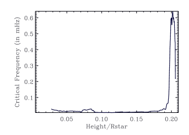
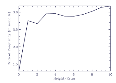
Figure 1: Radial profiles of the critical frequency in a solar or stellar chromosphere as predicted by semi-empirical models of $\alpha$ Tau (left ) and 31 Cyg (right ).

Reflection of Alfvén waves can play an important role in driving slow and massive winds from giants and supergiants (An et al. 1990; Airapetian et al. 1998, 2000, 2010; Suzuki 2007; Cranmer 2011). The radial profile of the critical frequency therefore provides important information about the role of the heating and momentum deposition of Alfvén waves in the atmosphere. The critical Alfvén frequency can be calculated directly from a semi-empirical model by differentiating the Alfvén velocity profile given by Eq. (2). Airapetian et al. (2013) have applied this procedure to the case of a K5 giant ($\alpha$ Tau) using the semi-empirical model of McMurry (1999). They showed that the Alfvén velocity gradient reaches its maximum at 0.21 $R_{\star}$. Figure 1 suggests that waves at frequencies less than 0.6 mHz are trapped in the chromosphere of $\alpha$ Tau (left panel). They also applied the same technique, based on the semi-empirical model developed by Eaton (2008), to calculate the gradient of the Alfvén velocity for the K5 supergiant primary in 31 Cyg. The right panel of Fig. 1 shows the vertical profile for $dV_{A}/dr$ in the chromosphere of 31 Cyg, and suggests that waves at $\nu\leq$ 3 nHz should be trapped in the first 10 stellar radii.

The magnetic field and the Alfvén velocity profile can also be probed by using the Poynting theorem (Jackson 1999):

$$\frac{\partial{W}}{\partial{t}}+\vec{\nabla}\vec{S}=-\vec{E}\vec{j},$$ (3)

where $W=\frac{1}{8\pi}(E^{2}+B^{2})$ is the electromagnetic energy density and $\vec{S}=\frac{1}{4\pi}~{}\vec{E}\times\vec{B}$ is the Poynting vector of the energy source. $\vec{S}$ represents the Poynting flux of Alfvén waves launched from the photosphere. For a steady-state chromosphere, $\frac{\partial{W}}{\partial{t}}$ = 0 and $\vec{S}$ has only an upward component $S_{z}$. We thus obtain

$$\frac{dS_{z}}{dz}=-<q>,$$ (4)

where $<q>$ is the time-averaged heating rate at a given height, $z$ (see also Song & Vasyliunas 2011).

The heating rate of the plasma can be derived from the energy equation for a steady-state chromosphere where the heating rate is balanced by the thermal conductive and radiative cooling rates, referred to as $L_{\rm cond}$ and $L_{\rm rad}$, respectively. It is found that

$$<q>=L_{\rm cond}+L_{\rm rad}.$$ (5)

In a stellar chromosphere, $T<0.5$ MK; the thermal conduction time is therefore much longer than the radiative cooling time, and the thermal conduction cooling term can be safely neglected. Consequently, the radial profile of the observationally derived cooling rates provides direct clues about the profile of the Poynting flux of the heating energy source. Detailed information about the radial profiles of the chromospheric magnetic field and the Alfvén velocity can be obtained if it is assumed that Alfvén waves are the major source of the chromospheric heating. The observations of non-thermally broadened chromospheric lines also imply that Alfvén waves may be the dominant source of energy and wind acceleration in cool giants and supergiants; further relevant discussions have been given by Airapetian et al. (2010) and by Cranmer & Saar (2011). This type of incompressible transverse wave can be directly excited, presumably through the shuffling or twisting of magnetic flux tubes by well developed magneto-convection in stellar photospheres (Ruderman et al. 1997; Musielak & Ulmschneider 2002). Recently, Morton et al. (2013) presented observational evidence that, in the solar photosphere, incompressible waves can be excited by the vortex motions of a concentration of magnetic flux.

The energy flux of Alfvén waves excited at the photosphere is defined by the $z$-component of the Poynting vector $\vec{S}=\frac{1}{4\pi}~{}\vec{E}~{}\times~{}\vec{B}$. By applying Ohm’s law, $\vec{E}=\eta\vec{j}-\vec{V}\times\vec{B}$, Ampere’s law, $\vec{j}=\frac{1}{4\pi}\vec{\nabla}\times\vec{B}$, and using vector identities, we can write the upward Poynting flux in Alfvén waves as

$$\vec{S}=\frac{1}{4~{}\pi}[\vec{V}~{}B^{2}-\vec{B}(\vec{V}\cdot\ \vec{B})]+\frac{\eta}{4\pi}(\vec{\nabla}\times\vec{B})\times{\vec{B}.}$$ (6)

If we further assume the existence of the azimuthal component only of the velocity of footpoint motions, $V_{\phi}\neq 0$, i.e., that there are no vertical motions in the photosphere (so $V_{z}=0$), and if we represent the total magnetic field as the sum of the background longitudinal flux-tube magnetic field $B_{z}$ plus the perturbed field $\delta{B}$ due to Alfvén waves, we obtain the $z$-component of the upward Poynting flux as

$$S_{z}=-\frac{1}{4~{}\pi}~{}B_{z}~{}V_{\phi}~{}{\delta B}-\frac{\eta}{4~{}\pi}{\delta B}\frac{\partial{\delta B}}{\partial{z}}.$$ (7)

For high magnetic Reynolds numbers, ${\rm Re}_{m}=\frac{V_{A}L}{\eta}$ ($\eta$ is the magnetic diffusivity), in the stellar chromosphere ($>$ 10, the second term in Eq. (7) can be neglected with respect to the first term. Then, following the Wallén relation $\delta V_{A}=\delta\frac{B}{\sqrt{4\pi\rho}}$ and assuming that waves are incompressible (so $\delta\rho$ = 0), we obtain

$$\frac{\delta{V}}{V_{A}}=\frac{\delta{B}}{B_{z}}.$$ (8)

This assumption is valid until Alfvén waves become strongly non-linear and convert a significant fraction of their energy into longitudinal waves (Ofman & Davila 1997; Suzuki 2007; Airapetian et al. 2014). Substituting $\delta B$ from Eq. (8) into Eq. (7), we obtain the Poynting flux as

$$S_{z}=\rho~{}<\delta V^{2}>V_{A}.$$ (9)

Furthermore, when combining Eqs. (4), (5), and (9), we obtain the following:

$$\frac{d}{dz}(\rho~{}<\delta V^{2}>V_{A})=-L_{\rm rad}(z),$$ (10)

Equation 10 relates the thermodynamic quantities such as the plasma density, turbulent velocity and the radiative cooling rates, which are obtained from semi-empirical models, to the hitherto unknown vertical profile of the Alfvén velocity. Equation 10 can be rewritten as:

$$e_{A}~{}\frac{dV_{A}}{dz}+\frac{de_{A}}{dz}~{}V_{A}=-L_{\rm rad},$$ (11)

where $e_{A}=\rho~{}<\delta V^{2}>$ is the energy density of Alfvén wave energy.

Once $V_{A}$ is known, the profile of the magnetic field throughout the chromosphere can be determined. Hence, the knowledge of $V_{A}$ and subsequent retrieval of $B_{z}(z)$ represents the missing link between thermodynamic-based semi-empirical models and MHD-based theoretical models of chromospheres and winds. This last equation allows us to determine the range of critical frequencies at which Alfvén waves become reflected from regions where the Alfvén velocity gradient is at a maximum.

Comparing the magnetic-field profiles derived from Eq. (11) with the one obtained from Eq. (1) enables us to determine the degree of deviation of the magnetic field in a chromosphere from the longitudinal (untwisted) magnetic field, thus allowing us to constrain the value of the azimuthal magnetic field. The magnetic-field profile in the chromosphere of $\alpha$ Tau as derived decreases with height at the rate of a super-radial expansion factor, $f(r)$. Then, the magnetic field varies with the height, $r$, as $B(r)\sim f(r)/r^{2}$, which is less steep than the profile obtained by Kopp & Holzer (1976) for solar coronal holes.

The next generation of semi-empirical models of evolved stars should therefore combine high-resolution spectroscopic and spatial information. Eclipsing binaries offer a unique opportunity to derive geometric constraints on the observed chromospheres and their winds (Eaton et al. 2008). Another promising approach utilizes high spatial-resolution interferometric observations of various giant and supergiant stars.

2.2 Momentum Deposition Requirements

The momentum deposition from non-radiative energy sources into stellar winds should explain the observed energy fluxes. An estimate of the energy flux that should be added in order to drive a steady-state wind above the atmospheric base can be derived from the energy equation for a steady-state wind in a single-fluid hydrodynamic approximation:

$$F_{\rm wind}=\frac{(-\dot{M})}{4\pi~{}R_{\star}^{2}}~{}(V_{\infty}^{2}+V_{\rm esc}^{2}).$$ (12)

$\rho$ is the wind mass density, $V_{\infty}$ is the wind terminal velocity, which is reached at radius $R_{\star}$, and $V_{\rm esc}$ is the escape velocity of the star at its surface (Holzer 1987). Detailed examination of chromospheric emission lines of Fe ii, O i and Mg ii indicate that the wind from a giant appears to originate near the base of the chromosphere and continues to accelerate throughout the entire chromospheric region (Carpenter et al. 1995). It is therefore assumed that the wind reaches its terminal velocity within one stellar radius, i.e., $R_{0}=R_{\star}$.

Table 1 presents radii, $R_{\star}/R_{\odot}$, escape velocities, $V_{\rm esc}$, wind velocities, $V_{\infty}$, and mass loss rates, $\dot{M}$, for selected stars (Robinson et al. 1998; Eaton 2008; Harper 2010; Neilson et al. 2011). One can see that a significant portion (from 65 to 95%) of the mechanical energy is required to lift the plasma beyond the gravitational well of the star and form the wind.

The energy flux required to generate the winds from $\alpha$ Tau, $\alpha$ Ori and 31 Cyg are $2.8\times 10^{3}$, $2.2\times 10^{5}$ and $2.5\times 10^{5}$ ergs cm^-2 s^-1. That suggests that in non-coronal giants, $F_{\rm wind}$ is only a few percent of the outer atmospheric heating rate and therefore over 90% of the energy flux of the mechanical source is trapped in the chromosphere while only a small fraction leaks out to accelerate and heat the wind. For supergiants the wind is initiated in much higher regions of the extended atmosphere; it reaches its terminal velocity before leaving the chromosphere (see Carpenter & Robinson 1997).

Another requirement for models of stellar winds arises from the constraints to the terminal wind velocities and mass-loss rates. For example, non-coronal giants and supergiants, including those in $\zeta$ Aur systems, show evidence of the presence of slow (a few tens of km s^-1) and massive winds. Models of steady-state, spherically-symmetric winds suggest that in order to produce the low terminal velocities (ones that are less than half the surface escape velocities) and the high mass-loss rates, most of the energy and momentum should be deposited below the sonic point, while momentum addition beyond the sonic point should produce the fast and tenuous solar-like winds (Hartmann & MacGregor 1980; Holzer 1987).

2.3 Constraints from Atmospheric Turbulence and Flows

High-resolution spectroscopy of many cool giants and supergiants has demonstrated that the profiles of optically thin UV lines of C ii], Si ii, Si iv and C iv that arise in the plasma that constitutes the chromosphere and transition regions in those stars show direct evidence of strong turbulence. The C ii] line is formed at temperatures between 5,000 and 10,000 K, and is optically thin in all of the stars observed. It has an intrinsically narrow profile, so the line width primarily reflects the Doppler broadening; the enhanced wings of the line profiles can be simulated by a single Gaussian profile (Carpenter et al. 1991). The deduced turbulent velocities range from 24 km s^-1 for the K5 giant $\alpha$ Tau to 35 km s^-1 for the M1.5 supergiant $\alpha$ Ori, thus suggesting supersonic turbulence in their chromospheres; see also discussions by Cuntz (1997), Robinson et al. (1998) and Cuntz et al. (2001). Many of the UV line profiles can be fitted by narrow and broad Gaussian components, as discussed by Wood et al. (1997), Dupree et al. (2005) and Eaton (2008). For example, fitting the profiles of C ii] in the M3.5 III star $\gamma$ Cru requires a two-component Gaussian model with FWHM = 27 and 42 km s^-1, and for $\alpha$ Ori, 19 and 48 km s^-1 (Eaton 2008).

Hybrid and coronal giants show much larger non-thermal velocities in transition region lines reaching 200 km s^-1, and also show narrow and broad Gaussian components. Moreover, non-thermal broadenings of UV lines observed in quiescent spectra of coronal giants as well as active dwarfs including the Sun tend to increase with temperature (Ayres et al. 1998; Pagano et al. 2004; Peter 2006).

Our Sun also shows non-thermally broadened, two-component Gaussian-shaped, red-shifted UV lines that form in the transition region (Peter 2006). That study does not confirm the idea suggested by Wood et al. (1997) and Pagano et al. (2004) that the broad component of UV lines is heated by microflares. In contrast, it used the spectrum of the Sun’s integrated disk to demonstrate that the broad components indicate the structure of its chromosphere. Carpenter & Robinson (1997) suggested that broad components may be a misleading description of the physics of a stellar chromosphere; instead of fitting the profiles by two Gaussian curves, they explain the enhanced wings by a signature of large-scale turbulence, which is anisotropically distributed along the line of sight and is directed preferentially either along, or perpendicular to, the radial direction. Airapetian et al. (1998, 2000, 2010) developed a 2.5-D MHD model of a stellar wind in which supersonic turbulent motions that are responsible for non-thermal broadening in the UV lines can be attributed to unresolved motions of the upward propagating non-linear Alfvén waves. The anisotropy formed by a large-scale longitudinal (open) magnetic field in an atmosphere can contribute to the formation of broad wings such as those observed in evolved giants and supergiants. Another important feature of the outer atmospheres of cool stars like the primary of 31 Cyg is the clumping of the gas, as proposed by Eaton (2008) and discussed further by Harper (2010).

Optically thin chromospheric lines from these stars and the Sun also exhibit a net redshift. This red-shift is indicative of downward motions of a few km s^-1 in non-coronal giants, and up to 30 km s^-1 in coronal giants as observed in lines from the chromosphere and transition region (Peter & Judge 1999; Ayres et al. 1998; Robinson et al. 1998; Doyle et al. 2002; Eaton 2008). It is interesting to point that Doyle et al. (2002) has observationally shown that the red Doppler shifts in the solar emission lines of O III, O IV and Ne VIII show short (a few minutes) variability. This time scale is comparable to the characteristic period of MHD waves observed in the solar chromosphere with the period of a few minutes (see Morton et al. 2012). Assuming that MHD waves are excited by magneto-convective motions with the turbulent turnover time of a convective cell, $\tau=L_{g}/V_{conv}$, we can expect a variation of red-shift shifts in chromospheric lines of red giants at the time scale of a few days. Judge & Carpenter (1998) concluded that such turbulent motions indicate downward propagating non-linear waves in the chromosphere. 3-D MHD models of the transition region in the Sun also interpret the observed emission-line red-shifts in terms of downward propagating compressive waves (Hansteen 1993), or material heated within low-lying transition-region loops that later cool and fall down into the chromosphere (Guerreiro et al. 2013). This process can be very important in the chromospheric dynamics and the energy balance, and therefore, provide a clue to the solar and stellar atmospheric heating. Can those models be incorporated into describing the mechanisms for heating chromospheres and winds? Thus, non-thermal broadening and redshifts of chromospheric lines represent one of the major signatures of chromospheric heating that need to be addressed by any viable theoretical model.

3 Acoustic Heating: Successes and Limitations

3.1 Two-Component Chromosphere Models

Following previous reviews by, e.g., Narain & Ulmschneider (1990, 1996), including references therein, particularly the work by Schrijver (1987) and Rutten et al. (1991), it has become obvious that from a general point of view stellar chromospheres can be considered as consisting of acoustically heated and magnetically heated components. The general heating rate, proliferated to stellar chromospheres including those of non-coronal giants and supergiants, can thus be expressed as

$$F\ =\ F_{\rm ac}(T_{\rm eff},g_{\star},Z)+F_{\rm mag}(T_{\rm eff},g_{\star},Z,P_{\rm rot}),$$ (13)

where $F_{\rm ac}$ is the acoustic heating rate and $F_{\rm mag}$ is the magnetic heating rate. Both increase as function of stellar effective temperature $T_{\rm eff}$, increase with decreasing stellar surface gravity $g_{\star}$ (i.e., by a few orders of magnitude between main-sequence stars and low-gravity supergiants), and also show some dependence on the stellar metallicity $Z$, which is however much less important than the impact of $g_{\star}$.

The magnetic heating rate also depends—at least in a statistical sense—on the rotation rate of the star, i.e., it is lower for slow rotating (i.e., older) stars, especially giants and supergiants, which have evolved away from the main-sequence (i.e., Schrijver 1993). This behaviour has profound consequences for the resulting amounts of chromospheric emission (e.g., Skumanich 1972; Noyes et al. 1984; Simon et al. 1985; Strassmeier et al. 1994), as identified in multiple spectral regimes, including detailed observations of Ca ii and Mg ii. The latter have been interpreted based on empirical, semi-empirical and theoretical concepts, including statistical relationships, and have also been utilized to decipher information about the thermodynamic, (magneto-)hydrodynamic and radiative properties of stars at different ages and evolutionary status. Detailed analyses focused on non-coronal giants have been described by Schrijver (1993), Schrijver & Pols (1993), and others. Furthermore, theoretical studies for the linkage between stellar atmospheric and wind properties, on the one hand, and the evolution of stellar dynamos, on the other hand, which actually constitute the physical reason for the fundamental changes, as the transition from coronal main-sequence stars to non-coronal giants, were given by MacGregor & Charbonneau (1994) and Charbonneau & MacGregor (1995).

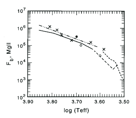
Figure 2: The basal flux limit for Mg ii h+k is shown as a function of effective temperature and compared to results from observations. The solid line represents the results of Rutten et al. (1991), and the double-dotted/dashed line the earlier ones from Schrijver (1987). The long-dashed line shows the upper limits derived for very cool dwarfs (Doyle et al. 1994). The short-dashed line is the Mg ii basal flux limit for giants (Judge & Stencel 1991). The crosses and open circles represent theoretical results from the present work, for main-sequence stars and giants, respectively. The closed circle at log $T_{\rm eff}$ = 3.70 is the theoretical result of Cuntz et al. (1994) but ignores the small differences in the Mg ii flux due to the different atmospheric metallicities considered (modified version of figure 5 of Schrijver 1995). (From Buchholz et al. 1998.)

Another pivotal aspect concerns the study of one-component (acoustic only) and two-component (i.e., acoustic and magnetic) chromospheric heating simulations itself. Detailed theoretical models for stars of different spectral types as well as non-coronal giants have been given by Ulmschneider (1989), Buchholz et al. (1998), Cuntz et al. (1998, 1999), and Fawzy et al. (2002). For example, Buchholz et al. (1998) presented 1-D time-dependent models of acoustically heated chromospheres for main-sequence stars between spectral type F0 V and M0 V and for two giants akin to spectral type K0 III and K5 III. The emergent radiation in Mg ii h+k and Ca ii H+K was calculated and compared with observations. They found good agreement, over nearly two orders of magnitude, between the time-averaged emission in these lines and the observed basal flux emission, which had been suspected to be due to nonmagnetic (i.e., acoustic) heating operating in all late-type stars. The authors pointed out that the results obtained clearly support the idea that the ‘basal heating’ of the chromospheres of late-type stars, including non-coronal giants (see Fig. 2) is due to acoustic waves. The latter result has been disputed in the meantime (Judge & Carpenter 1998) from the view of that acoustic wave heating, in the context of existing models, is unable to explain the amounts of observed turbulence (see Sect. 2.3).

3.2 Possible Relevance of Acoustic Waves for Winds from Cool Evolved Stars

An important feature of acoustic waves in stellar atmospheric environments, including the chromospheres of evolved giants and supergiant stars, is that they dissipate the lion’s share of their mechanical energy flux fairly close to the stellar photospheres; see, e.g., the study of Ulmschneider (1989) that compared the dissipative behaviour of acoustic waves in giants and dwarfs of identical effective temperatures. This key result about the dissipative properties of acoustic waves in cool evolved stars, implying that acoustic waves cannot support the massive winds of those stars, has also been discussed in the broader context of proposed stellar mass loss mechanisms by Holzer (1987). Thus, this entails an additional justification for the exploration of Alfvén wave driven winds for non-coronal evolved stars as opposed to nonmagnetic mechanisms. Alfvén wave driven wind models were pursued by Hartmann & MacGregor (1980), Hartmann & Avrett (1983), and more recently by, e.g., Airapetian et al. (2014). A detailed study by Cuntz (1990), focused on $\alpha$ Boo (K2 III) and based on adequate acoustic wave frequency spectra, yielded acoustically initiated mass loss rates on the order of $10^{-13}$ to $10^{-15}$ $M_{\odot}$ yr^-1, which are more than a factor of 10⁴ below the observationally established limit.

The decisive shortcoming of acoustic waves consists in that they fail to dissipate their mechanical energy over a significant distance that is comparable to the height of the critical point (Holzer & MacGregor 1985; Cuntz 1990; Judge & Stencel 1991). This property thus leads to absurdly low mass loss rates due to acoustic waves. Previous relatively positive assessments about the ability of acoustic waves to drive mass loss from evolved stars were given by Pijpers & Hearn (1989). They explored a simple stellar wind model loosely guided by the stellar parameters of $\alpha$ Ori, which led to mass loss rates in the range between 10^-8 and 10^-4 $M_{\odot}$ yr^-1, depending on the wave parameters, which at first sight appear to be promising. However, this type of model must be ruled inapplicable as it is based on the assumption of time-independent and linear behavior of the acoustic waves, excluding, for example, the possibility of shock formation. Thus the results that were obtained then carry little meaning.

Nevertheless, acoustic waves are still expected to be relevant for initiating mass loss from non-coronal giants and supergiant stars as they are able to increase the thermal pressure and density scale heights in the spatially extended chromospheres owing to their dissipative behaviors (i.e., heating and transfer of wave pressure), see Buchholz et al. (1998) and references therein. Another possible contribution of nonmagnetic processes is the initiation of turbulent pressure that may help to lift matter closer to the critical point of the stellar wind as pointed out by, e.g., Suzuki (2007). Detailed assessments, in the framework of 1-D models, of acoustically generated turbulence in chromospheric models of $\alpha$ Tau show however that the synthetic results are significantly lower than those obtained by GHRS observations (Judge & Cuntz 1993). However, it is still an unsettled debate (see Judge & Carpenter 1998; Cuntz et al. 2001) whether this discrepancy is due to the unrealistic 1-D assumption of existing theoretical models, or whether it is more profoundly enshrined in the basic physics of acoustic processes. Preliminary 3-D models of convectively initiated turbulence in case of $\alpha$ Ori have been given by Freytag et al. (2002).

4 MHD Wave Driven Heating and Wind Acceleration

4.1 Energy Dissipation Due to Alfvén Waves: A Source of Chromospheric Heating

Magnetic heating mechanisms for solar and stellar chromospheres have been targeted in numerous reviews, including those by Narain & Ulmschneider (1990, 1996). Two major types of heating mechanisms have generally been proposed, which are broadly classified as AC (i.e., alternating current, such as MHD wave dissipation) and DC (i.e., direct current, such as magnetic-field dissipation through magnetic reconnection). In this review we focus on the progress regarding AC heating processes and their observational signatures. MHD-wave heating can be driven by two types of waves: compressible longitudinal MHD waves (slow and fast magneto-sonic waves), and incompressible transverse waves (i.e., torsional Alfvén waves). According to Ulmschneider et al. (2001) and Musielak & Ulmschneider (2002), the energy fluxes of longitudinal and transverse waves in cool evolved stars are comparable, and are of the order of $10^{7}-10^{8}$ ergs cm^-2 s^-1. That amount of energy generated by waves in stellar photospheres of cool giants is sufficient to account for the observed cooling rates together with the energy needed to drive winds (see Sect. 2.1.

Torsional Alfvén waves have been suggested as a likely source for the heating of the solar chromosphere and corona (Osterbrock 1961; Hollweg 1973, 1978; Heinemann & Olbert 1980; Holzer et al. 1983; Cranmer & Ballegooigen 2005; Mathioudakis et al. 2013). That approach has also been extended to the outer atmospheres of cool evolved stars (Hartmann & MacGregor 1980; Holzer et al. 1983; Hartman & Avrett 1984; Suzuki 2007, 2013; Cranmer 2008, 2009).

Alfvén waves can damp energy in solar and stellar atmosphere through a number of mechanisms. For example, in closed magnetic structures resonant absorption mechanism may become efficient, while in closed and open structures energy dissipation through the cascade due to Alfvén wave turbulence or mode conversion may become efficient (Davila 1987; Matthaeus et al. 1999; Cranmer & Ballegooigen 2005; Suzuki & Inutsuka 2005; Mathioudakis et al. 2013; Airapetian et al. 2014). Studies by An et al. (1990), Barkhudarov (1991), Rosner et al. (1991), Velli (1993), MacGregor & Charbonneau (1994) and Charbonneau & MacGregor (1995) concluded that as waves propagate in a gravitationally-stratified atmosphere they may become subject to reflection from atmospheric regions where the gradient in the Alfvén velocity is comparable to, or greater than, the Alfvén wave frequency.

While those studies clearly point to the possible importance of magnetic-wave pressure in chromospheric heating, they suffer from the restrictive nature of the linearity assumptions as well as from the fact that they are not consistently solving the relevant MHD equation involving the magnetic field, density and velocity. Although the linear treatment of winds in cool, luminous stars has shown that MHD turbulence can be important for driving the winds, those models are incapable of examining properly the wave dissipation—a critical part of the mechanism. Furthermore, because the entire set of non-linear time-dependent MHD equations is not solved consistently in those studies, there is the possibility that important physical effects are neglected or overlooked. An important example is that the coupling between the azimuthal and radial components of the velocity and magnetic fields are only treated in a linear approximation. Recent models by Suzuki (2007, 2013) treat self-consistently the dissipation of Alfvén waves in forming stellar chromospheres and coronal layers that expand into winds, but they assume that Alfvén waves are launched from a fully-ionized photosphere—an approximation that is not applicable, since the degree of ionization in giant and supergiant photospheres is less than 10^-5, and is less than 1 in most parts of the chromosphere. That approach therefore overlooks a wide range of physical effects of wave dissipation in a partially-ionized magnetized plasma.

In a weakly ionized medium such as a stellar chromosphere, where there is varying collisional coupling between ions and electrons throughout, new effects can appear, such as the non-ideal Hall effect or ambipolar diffusion. In astrophysics, ambipolar diffusion usually refers to the decoupling of neutral and charged particles in a plasma. If both electrons and ions are magnetized (or frozen-in into the magnetic field), neutral particles do not ‘feel’ the magnetic field and will slip through it. Neutral particles then drag ions with them via ion–neutral collisions, introducing an electric field perpendicular to the magnetic field lines. The Hall effect occurs when electrons are magnetized but ions are not. In such a case the Hall electric field results from the drift velocity of electrons with respect to ions, because the two kinds of charged particles respond differently to collisions from the neutral particles. In solar and stellar atmospheres the ambipolar diffusion perpendicular to the magnetic field is many orders of magnitude greater than the classical Spitzer diffusion along the magnetic field. The collisional coupling between charged particles and neutral gas is therefore a fundamental process in weakly ionized and strongly magnetized solar and stellar chromospheres and winds (Piddington 1956; Osterbrock 1961; Hartman & MacGregor 1980; Holzer et al. 1983). Many recent studies (Goodman 2000, 2004; De Pontieu et al. 2001; Khodachenko et al. 2004; Leake et al. 2005; Krasnoselskikh et al. 2010; Soler et al. 2013; Tu & Song 2013) have shown that in the solar chromosphere, which is a weakly ionized and magnetized atmosphere, the effect of ion–neutral collisions becomes significant in dissipating the electric currents introduced by MHD waves.

Airapetian et al. (2014) recently showed that the effects of ambipolar diffusion may also play a crucial role in the chromospheres of cool giants. It is known that the photospheres of cool giants and supergiants are characterized by well-developed magneto-convection with characteristic velocities up to 10 km s^-1 (Gray 2008; Chiavassa et al. 2010). Interaction of such motions with open magnetic fields may excite longitudinal and transverse MHD waves. What happens is that transverse Alfvén waves cause periodic fluctuations of plasma motions perpendicular to the magnetic field lines and thereby induce an electric field, $\vec{E}=\vec{\delta V}\times\vec{B}/c$, in the reference frame of the plasma. This induced electric field generates electric currents. The dissipation of the currents induced by the Alfvén waves perpendicular to the magnetic field provides an efficient source for converting the kinetic energy of convection into electrical energy. Working from the approach of Braginskii (1965), De Pontieu & Haerendel (1998), De Pontieu et al. (2001), Goodman (2004), Leake et al. (2005), Leake & Arber (2006) and Tu & Song (2013), Airapetian et al. (2014) developed MHD models of Alfvén-wave heating for a partially ionized plasma in a solar or stellar chromosphere. A key component of those types of models is the inclusion and self-consistent calculation of the anisotropic electrical conductivity tensor.

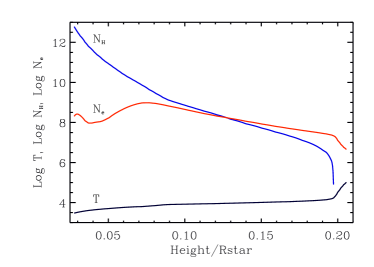
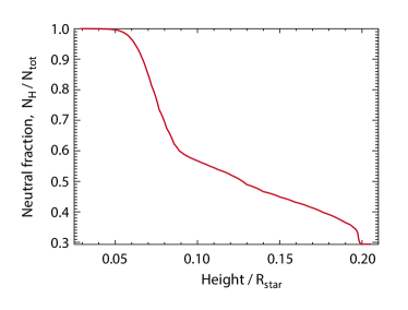
Figure 3: Chromospheric model of $\alpha$ Tau. Left: radial profiles of $T$, $N_{H}$, $N_{e}$. Right: radial profile of neutral fraction $N_{H}/N_{\rm tot}$.

To describe the role of ambipolar diffusion and the Hall effect in the chromosphere of a cool evolved star we need to know how the thermodynamic parameters of the atmosphere vary with height. Those parameters are provided by semi-empirical models of the chromosphere, complemented by the magnetic-field profiles (see Sect. 2.1). In the following, as an example we focus on McMurry’s semi-empirical model for $\alpha$ Tau. We also consider that the chromosphere has a longitudinal but vertically diverging magnetic field, $B_{z}=B_{0}~{}(R_{\star}/r)^{2}$, where $B_{0}$ = 20 G. The upper left panel of Fig. 3 shows the radial profile of the chromospheric temperature, electron number density and N_H (the sum of the neutral and ion densities). The upper right panel presents the radial profile of the neutral fraction, $n_{H}/n_{\rm tot}$, and the lower one shows the vertical profile of the plasma beta, $\beta=P_{\rm gas}/P_{\rm mag}$. The magnetic pressure appears to be dominant in most of the chromosphere.

In a partially ionized plasma consisting of electrons, protons and neutral particles, the motions of charged particles are strongly affected by electron-neutral and ion–neutral collisions. In such a highly collisional plasma of a stellar chromosphere, neutral hydrogen, electrons and protons are efficiently coupled, thus constituting a single fluid if the electron-ion collision frequency is greater than the characteristic frequency of the waves propagating through the medium. This approximation is valid for low-frequency Alfvén waves (less than 1 Hz) in a chromosphere. Electrons and protons gyrate along the magnetic field with characteristic frequencies of $f_{ce}=2.8\times 10^{6}$ $B$ for electrons and $f_{cp}=1.52\times 10^{3}$ $B$ for protons. For a longitudinal magnetic field of 100 G, such frequencies are in the range $10^{5}-10^{8}$ Hz.

Unlike fully ionized plasmas, the photosphere and chromosphere of a red giant contain a large fraction of neutral species that collide with electrons and ions at frequencies $f_{en}$ and $f_{in}$, respectively. They are given as

$$f_{en}=1.95\times 10^{-10}~{}n_{H}~{}\sqrt{T},$$ (14)

$$f_{pn}=7.87\times 10^{-11}~{}n_{H}~{}\sqrt{T},$$ (15)

and are found to vary within a frequency range of $10^{2}-10^{4}$ Hz. Consequently, over the entire range of relevant heights in the atmosphere, the electron and ion gyrofrequencies exceed the proton-neutral and electron-neutral collision frequencies. This means that both electrons and ions are magnetized throughout the chromosphere. It also suggests that the Hall effect is negligible for chromospheric conditions, but—according to Goodman (2000)—it is important in the lower parts of the solar chromosphere. Mitchner & Kruger (1973) showed that in plasmas where the magnetization of electrons, $M_{e}$, and ions, $M_{i}$ (i.e., the ratio of electron or ion gyrofrequency to the total collision frequency of electrons or ions with neutral particles), becomes greater than 1, the plasma conductivity becomes anisotropic. First, this requires that the Spitzer resistivity, which is parallel to the magnetic field, needs to be modified from its fully ionized value from electron-neutral collisions. Secondly, it also requires including the perpendicular component of the anisotropic electrical resistivity tensor (the Pedersen resistivity), which is described by

$$\eta_{\rm per}=\frac{[(1+\Gamma)^{2}+M_{e}^{2}]}{(1+\Gamma)\eta_{\rm par}}\\$$ (16)

$$\eta_{\rm par}=\frac{M_{e}(f_{ei}+f_{en})}{n_{e}~{}c^{2}}\\$$ (17)

$$\Gamma=(\frac{n_{H}}{n_{\rm tot}})^{2}~{}M_{e}~{}M_{i}\\$$ (18)

$$M_{e}=\frac{f_{ce}}{f_{ei}+f_{en}},~{}~{}M_{i}=\frac{f_{ci}}{f_{i}},\\$$ (19)

where $f_{i}=\frac{m_{H}}{m_{i}+m_{h}}$. $\eta_{\rm par}$ is the Spitzer resistivity that applies along the magnetic field and $\eta_{\rm per}$ is the Pedersen resistivity perpendicular to it.

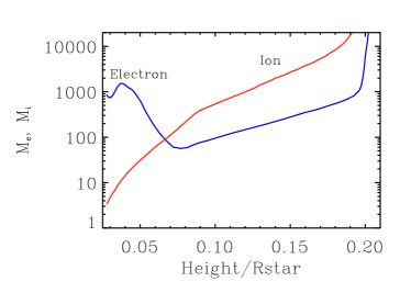
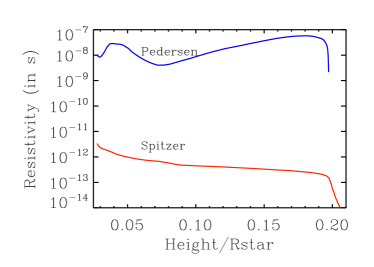
Figure 4: Chromospheric model of $\alpha$ Tau. Left: radial profiles of electron and proton magnetizations throughout the chromosphere. Right: Spitzer and Pedersen resistivity throughout the chromosphere.

The left panel of Fig. 4 shows that the photospheric and chromospheric plasma is weakly ionized but strongly magnetized for both electrons and ions, and therefore that $\Gamma\gg 1$ for a longitudinal photospheric magnetic field of 20 G. That suggests that the role of the Hall effect should be negligible in the atmosphere.

The Pedersen resistivity is given as

$$\eta_{\rm per}\propto\Gamma~{}\eta_{\rm par}\propto\frac{B_{z}^{2}}{n_{H}^{2}~{}\sqrt{T}}.$$ (20)

The right panel in Fig. 4 shows that the Pedersen resistivity is dominant throughout most of the solar chromosphere and through the entire chromosphere of giants and supergiants. Pedersen resistivity is $4-6$ orders of magnitudes greater than the Spitzer resistivity, and it should therefore be critical for the heating rates introduced by the dissipation of electric currents that are induced by the transverse motions of Alfvén waves. This result also means that the less stratified chromospheres of giants and supergiants (i.e. less surface gravity) will reduce the density of the chromospheric plasma and therefore increase the significance of the Pedersen resistivity relative to the chromospheres of dwarf stars.

This approach was recently applied to model chromospheric heating in red giants (Airapetian et al. 2014). They employed a 1.5-D MHD code with a generalized Ohm’s law and McMurry’s semi-empirical model for $\alpha$ Tau to simulate the propagation of harmonic Alfvén waves at a single frequency of 0.01 mHz. The single fluid fully non-linear resistive and viscous MHD equations were treated for partially-ionized plasma according to

$$\frac{\partial\,\rho}{\partial\,t}+\nabla\cdot\left(\rho\,\vec{V}\right)=0,$$ (21)

$$\rho\left[\frac{\partial\,\vec{V}}{\partial\,t}+\left(\vec{V}\cdot\nabla\right)\,\vec{V}\right]=-\nabla\,p+\rho\vec{g}+\vec{J}\times\vec{B}+\nabla\vec{S}$$ (22)

$$\frac{\partial\,\vec{B}}{\partial\,t}=-\nabla\times\vec{E},$$ (23)

$$\vec{E}=-\vec{V}\times\vec{B}+\left(\eta_{\rm par}\vec{J}_{\rm par}+\eta_{\rm per}\vec{J}_{\rm per}\right),$$ (24)

$$\frac{\partial\,(\rho E)}{\partial\,t}+\nabla(\rho E\vec{V})=-P\nabla{\vec{V}}+\left(\eta_{\rm par}\vec{J}_{\|}^{2}+\eta_{\rm per}\vec{J}_{\bot}^{2}+\zeta_{ij}S_{ij}-L_{\rm rad}\right)$$ (25)

$S_{ij}$ denote the components of the stress tensor $\vec{S}=\nu[\zeta_{ij}-(\delta_{ij}\nabla{\vec{V}})/3]$ and $\zeta_{ij}=\frac{1}{2}(\frac{\partial\,V_{i}}{\partial\,x_{j}}+\frac{\partial\,V_{j}}{\partial\,x_{i}})$; $\nu=\nu_{\rm nn}+\nu_{\rm in}$ is the viscosity coefficient due to neutral–neutral and ion–neutral collisions (Leake et al. 2013), $E$ is the specific internal energy, given by $E=\frac{P}{\rho(\gamma-1)}+(1-\xi_{n})\frac{X_{i}}{m_{av}}$, $L_{\rm rad}$ is the total radiative cooling rate; other variables have their usual meaning. The method of solving the continuity, momentum and induction equations in a partially ionized plasma has been described in detail by Arber et al. (2001) and Leake & Arber (2006).

A steady-state flux of Alfvén waves is launched from the photosphere along a vertically diverging flux tube (Airapetian et al. 2014). The initial Poynting flux of Alfvén waves is given as $F_{A}=4\times 10^{7}$ ergs cm^-2 s^-1. As waves propagate upward along the magnetic field lines into the stellar chromosphere, the wave amplitude grows as the density falls with height. Figure 5 shows that the amplitude of Alfvén waves increases by a factor 10 at $t=0.3~{}t_{A}$, where $t_{A}$ is the Alfvén transit time. Such an amplitude of unresolved turbulence formed by Alfvén waves is consistent with the non-thermal broadening that is observed in UV lines.

One important feature revealed by the simulations of these non-linear transverse waves is their conversion into longitudinal (compressible) waves. This conversion occurs at the altitude ($\geq$ 0.05 $R_{\star}$) at which the sound speed becomes equal to, or greater than, the Alfvén speed (upper right panel of Fig. 3). At the narrow layers where plasma $\beta\sim$ 1, non-linear transverse Alfvén wave motions become strongly coupled to compressible wave motions or slow magneto-sonic waves (left panel of Fig. 6). The wave mode conversion is revealed by the formation of non-linear density fluctuations at amplitudes as high as 50% of the unperturbed density, starting at 0.05 $R_{\star}$ and propagating to the upper layers of the chromosphere as presented in the right panel of Fig. 4. At that altitude the wave Poynting flux is about 7 $\times$ 10⁵ ergs cm^-2 s^-1, and therefore over 70% of the surface energy flux is dissipated or reflected back to the chromosphere. The right panel of Fig. 6 shows that the total energy density reaches its first peak at 0.05 $R_{\star}$, suggesting the formation of non-linear slow magneto-sonic waves at an energy density of 0.25 ergs cm^-3 in narrow layers distributed in the chromosphere for up to 0.3 $R_{\star}$. The energy flux associated with compressible waves is 2 $\times$ 10⁵ ergs cm^-2 s^-1, which is $\sim$30% of the flux in the Alfvén waves. Highly non-linear, slow magnetosonic waves then steepen into shocks that are not resolved in the described simulations. The right panel also shows that the non-linear compressible waves dissipate their energy efficiently into heat in a narrow range of heights, from 0.05–0.4 $R_{\star}$. The effect of the dissipation of compressible waves is traced by the sharp drop of the compressible energy density in upward propagating waves.

The wave energy dissipates mostly via viscosity owing to neutral–neutral collisions and resistivity caused by ion–neutral collisions. The effect of mode coupling of the conversion of energy from Alfvén waves into slow magneto-sonic waves has also been observed and described in 1-D MHD simulations of the solar chromosphere by Lau & Siregar (1996), Torkelsson & Boynton (1998), Ofman & Davila (1997), Airapetian et al. (2000) and Suzuki (2013) in simulations of solar and stellar atmospheres and winds.

At this point, the Alfvén wave motions become non-linear and induce significant electric fields. The induced perpendicular component of the electric current (with respect to the vertical magnetic field) is then efficiently dissipated by Pedersen resistivity with the volumetric Joule heating rate, $\eta_{\rm per}J_{\rm per}^{2}$.

According to Airapetian & Carpenter (2013) (see also the left panel of Fig. 3), the McMurry model predicts a strong peak in the Alfvén velocity gradient that forms the reflection point at $\sim 0.2~{}R_{\star}$ for upward propagating Alfvén waves. The model shows that Alfvén waves with critical frequencies less than the critical frequency of $\nu_{\rm crit}=dV_{A}/dr=5\times 10^{-4}$ Hz get reflected down to the chromosphere and interact with outgoing Alfvén waves, thus introducing a velocity shear. This suggests that the chromosphere is a low-frequency filter that passes only the higher-frequency waves into the upper atmosphere (where they can be dissipated). The reflected non-linear waves initiate downflows in the chromosphere, which can potentially explain not only non-thermal broadening but also the redshifts that are observed in UV lines from cool evolved stars.

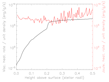
Figure 7: Model outputs. Left: viscous (black) vs Joule (red) heating in the chromosphere. Right: radial profile of the mass-loss rate at 0.3 $t_{A}$.

In a partially ionized plasma, the volumetric viscous heating rate is mostly caused by kinematic neutral–neutral viscosity in the presence of velocity shear, $H_{\rm visc}=0.5\zeta_{nn}(\nabla{\delta V})^{2}$. This term becomes important in the energy balance of the chromosphere when waves become strongly non-linear. The left panel of Fig. 7 shows that the viscous rate becomes comparable to the Joule heating rate in the mid-chromosphere. However, because the grid resolution is not high enough to allow us to resolve the viscous dissipation scales, viscous effects cannot be estimated consistently.

As non-linear waves propagate upward, they exert non-linear magnetic-pressure gradients upon the plasma, $\sim d(\vec{J}\times\vec{B})/dr$. This force is commonly known as the ponderomotive force. It has been shown that it may be responsible for accelerating the solar or stellar winds (see for example Ofman & Davila 1997, 1998; Airapetian et al. 2000, 2010).

The model by Airapetian et al. (2014) suggests that non-linear waves can deposit significant momentum and cause the mass loss that is consistent with observation. The right panel of Fig. 7 characterizes the momentum deposition in the chromosphere in terms of the mass-loss rate, $\dot{M}=\rho V_{r}r^{2}$ ($V_{r}$ is the radial velocity of the plasma, $r$ is radial distance), throughout the atmosphere at $t=0.3~{}t_{A}$. The plot shows that at the top of the chromosphere the mass loss rate becomes constant at about $10^{18}$ g s^-1 $\sim 10^{-8}~{}{\dot{M}}_{\odot}$ yr^-1 . It also suggests that the filling factor of the open magnetic field is about 0.1$\%$.

Future models should therefore also take radiative losses into account and calculate the profiles and fluxes of chromospheric lines formed in the model atmosphere (as discussed in Sect. 5). That requires knowledge about the heating rates that balance the radiative losses. In the 1.5-MHD simulations presented above, Airapetian et al. (2014) employed for the first time the high-resolution simulations that resolve structures at scales less than 1,500 km. The resolution of their grid allowed them to resolve resistive dissipation scales, and thereby yielded heating rates that were physically meaningful.

The numerical diffusivity is given by

$$D_{\rm num}=V_{A}\Delta^{2}/L,$$ (26)

where $\Delta$ is the numerical grid spacing, and L is the characteristic length of the physical structure. $D_{\rm num}$ reaches its largest value then the characteristic length equals the grid size, $V_{A}\Delta$. The Pedersen diffusivity,

$$D_{\rm Pedersen}=c^{2}\eta_{\rm ped}/4{\pi},$$ (27)

where $\eta_{\rm ped}$ is given by Eq. (21). The ratio of the Pedersen to the numerical diffusivity is therefore proportional to

$$\frac{D_{\rm Pedersen}}{D_{\rm num}}\propto\frac{B}{n_{H}^{2}\Delta\sqrt{T}}~{}.$$ (28)

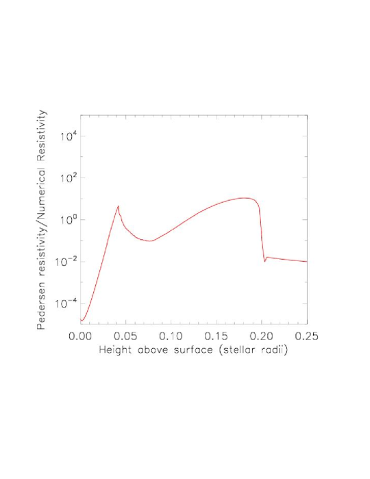
Figure 8: Model outputs. The vertical profile of the ratio of the Pedersen to the numerical resistivity in a 1.5-D MHD model by Airapetian et al. (2014).

Equation 29 suggests that in the regions of stronger magnetic fields (i.e. active regions), the ratio of physical to numerical resistivity increases. Indeed, Fig. 8 shows that the ratio of the Pedersen to the numerical resistivity is mostly greater than unity throughout most of the chromosphere of $\alpha$ Tau. That suggests that the calculated heating rates directly reflect the energy input into the plasma and can be used to calculate the radiative output from the chromosphere for direct comparison with observations.

4.2 Momentum Deposition by Alfvén Waves: Driving Winds from Cool Evolved Stars

The general requirements for the driver of winds from cool evolved stars include the condition for their initiation below the sonic point of the star, namely, $R_{s}={GM_{\star}}\,/\,{2V_{s}^{2}}\sim 10-20~{}R_{\star}$, where $V_{s}$ is the isothermal speed of sound (Holzer 1983). A more refined condition arises from the requirement of initiation and acceleration of winds—for example, in non-coronal giants within the first stellar radius and its association with the supersonically turbulent and clumpy chromosphere (Carpenter et al. 1995). Radiation pressure on the atmospheric plasma, which is generally accepted as the process driving massive winds from hot stars, is too small to account for what occurs in cool giant stars. Dust-driven effects in wind acceleration are not important in K and early-M giants, because there is no evidence for dust formation close to the star (Danchi et al. 1994). The second possible mechanisms, namely winds driven by acoustic waves, is also not capable of producing the required mass-loss rate (see the discussion in Sect. 3). The most promising mechanism to date for cool evolved stars requires MHD waves both to heat the plasma and to accelerate the wind.

The role of MHD waves in initiating and accelerating winds from numerous types of stars, including the Sun, solar-types and cool evolved ones, have been studied extensively since the early 1970s (Hollweg 1973, 1978; Heinemann & Olbert 1980; Hartmann & MacGregor 1980; Ofman & Davila 1998; Airapetian et al. 2000; Suzuki 2007; Cranmer 2008, 2009; Airapetian et al. 2010). The effects of 1-D non-linear Alfvén waves have been studied by Lau & Siregar (1996) and by Boynton & Torkelsson (1996). Moreover, 2.5-D self-consistent non-linear treatments of Alfvén waves for the solar wind and accelerations from coronal holes have also been performed (Ofman & Davila 1997; Ofman & Davila 1998). Grappin (2002) modelled a solar wind that was driven by 2.5-D MHD Alfvén waves and included both open and closed magnetic configurations. The above studies suggest that as initially small-amplitude torsional Alfvén waves, which are generated at the coronal base, propagate upward in a gravitationally-stratified atmosphere, they become non-linear and transfer momentum efficiently to the bulk plasma flows because of the vertical gradient of the magnetic wave pressure. Non-linear coupling of Alfvén waves excite magneto-sonic waves, which can eventually steepen into longitudinal waves that become damped by shock formation. Suzuki & Inutsuka (2005) and Suzuki (2007, 2013) pursued non-linear 1.5-D MHD simulations of Alfvén wave propagation from solar and stellar photospheres into the corona. While their model does not account for cross-field gradients, they showed that non-linear Alfvén wave dissipation in the solar atmosphere can explain its thermodynamics due to the dissipation of compressible waves produced by mode coupling of non-linear Alfvén waves.

Recent progress in our understanding and modelling of coronal solar and stellar winds driven by MHD waves provides a solid foundation to characterize such winds in the environments of magnetically-active solar-like and evolved luminous stars (Ofman & Davila 1997, 1998; Cranmer 2009; Airapetian et al. 2010; Cranmer & Saar 2011). If the hot, fast, tenuous winds from solar-like stars are driven by a combination of coronal gas pressure and Alfvén wave pressure, the cool massive winds emanating from cool evolved stars are also expected to be powered by Alfvén wave pressure; Airapetian et al. (2000, 2010, 2011) describe models of slow massive winds from late-type luminous stars. Future models should apply a single fluid MHD approximation to treat large-scale wind flows from magnetically open fields that extend from the base of the wind to 25 $R_{\star}$ and beyond. The validity of the MHD approximation is warranted by GHRS spectroscopic observations of wind plasmas that have electron densities of $10^{9}$–10¹⁰ cm^-3 and temperatures between 10,000 K and 1 MK. Because the magnetic field at the base of the wind is about 1–10 G, the ratio of the thermal to magnetic pressure in the plasma, or plasma-$\beta$, is less that unity at that level.

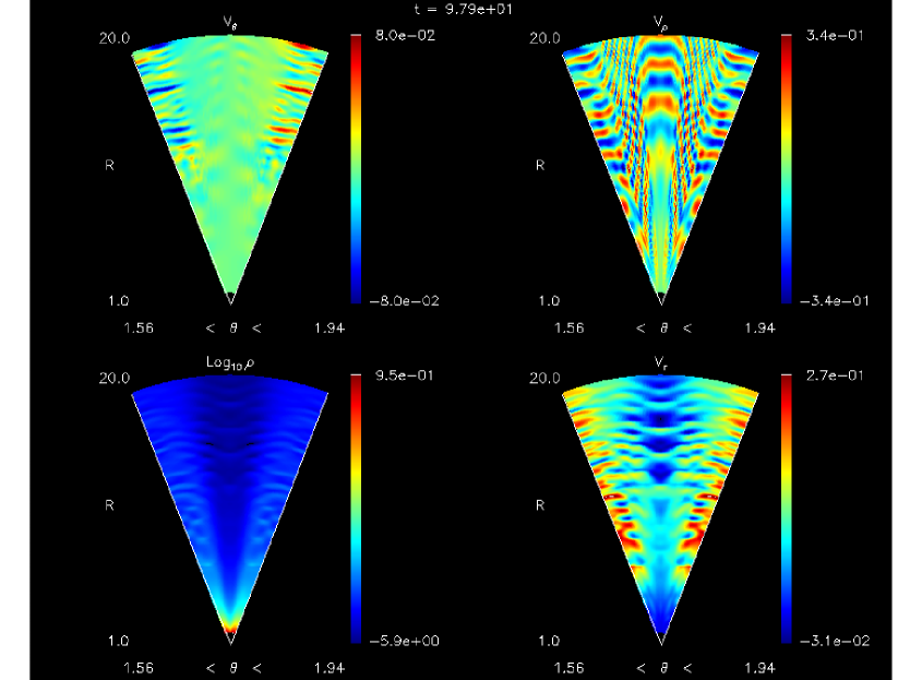
Figure 9: Variation of the radial and azimuthal velocities, $V_{\theta}$, $V_{\phi}$, $V_{r}$ and $\rho$ in a $r-\theta$ slice of a magnetically open region from 1–20 $R_{\star}$. The Alfvén waves are reflected at a height of $\sim 5.5~{}R_{\star}$, which thus marks the onset of the wind.

Previous models have described the propagation, in a gravitationally-stratified atmosphere, of non-linear Alfvén waves that are launched from a chromospheric hole at the base of the wind at a single frequency in two wind geometries, and applied it to giants and to supergiants such as $\alpha$ Ori (Airapetian et al. 2010). The results of those simulations suggest the formation of a two-component wind for giant stars from a magnetically open configuration that is dubbed a ‘chromospheric hole’. Figure 9 presents 2-D maps of the radial velocities in that model. It shows the formation of slow (0.1 $V_{A}$) and fast (at 0.22 $V_{A}$) components of the wind. While the fast component is formed outside the low-density region, the slow wind component emerges from the inner regions of the low-density regions and is about 10 times less dense.

This model showed that in order to explain the high mass-loss rate of $\alpha$ Ori, a surface magnetic field of 200 G must be assumed for its chromospherically active regions. Magnetic fields with an average surface distributed field of 1 G have recently been detected in this object (Petit et al. 2013). The finding suggests that the field can reach 200 G if the filling factor of the field is $\sim$0.5%.

Wind models have also been extended by adding a broad-band distribution of Alfvén waves that propagate in the atmosphere of late-type giants. To model the wind from a typical red giant (the example taken was that of $\alpha$ Tau, K5 III), well-constrained input model parameters were adopted (mass, radius, temperature, initial amplitude and spectral range of Alfvén waves launched at the base of the wind), together with output wind parameters inferred from observation (terminal velocity of the wind and mass-loss rate). In order to get a better constraint on the lowest end of the frequency spectrum of the Alfvén waves ($\nu_{1}$), the parametric dependence of $\nu_{1}$ on the mass-loss rate and wind speed were assessed by calculating four Alfvén wind models (Models A, B, C, and D) corresponding to various lowest frequencies $\omega_{1}$ = 1, 3, 9 and 18$\tau_{A}^{-1}$ (or wave periods of the Alfvén wave spectrum of 16.2, 5.4, 1.8 and 0.9 days, respectively) (Airapetian et al. 2010). At the outer boundary, open (non-reflecting) conditions for MHD waves were imposed in order to reach a quasi steady-state solution. Airapetian et al. (2010) solved MHD equations for a fully ionized plasma in order to to calculate the time-averaged terminal velocities and output mass-loss rates of quasi steady-state winds for Models A–D. Note that Model D ($\omega_{1}/\omega_{A}$ = 18), corresponding to freely propagating waves, drives faster and less massive winds. The total mass-loss rate from a stellar atmosphere filled by an open magnetic field is proportional to the surface magnetic flux (Eq. 11 of Airapetian et al. 2010). That equation suggests that the wind mass-loss rate should vary on timescales of the emergence and evolution of the magnetic flux associated with an open magnetic field, or on the timescale of the rotation period of the star. While the timescale of magnetic-field amplification by giant cell convection is of the order of 25 years (Dorch 2004), the rotation period of a typical giant is of the order of 1 year.

The fact that the wind forms in anisotropically distributed ‘active regions’ on the stellar surface also implies that the generated wind outflows should have anisotropic and clumpy structures. These predictions are consistent with observations of inhomogeneous chromospheres in red giants and supergiant stars (Eaton 2008; Ohnaka et al. 2013; Ohnaka 2013). Observations by Mullan et al. (1998) and Meszaros et al. (2009) suggest that the mass-loss rate in $\lambda$ Vel shows time variability by a factor of six, and by a factor of two in K341 (M15) and L72 (M13) over 18 months of observations.

More specifically, when the total mass-loss rate given by the model is compared with the measured rate for $\alpha$ Tau, the area filling factor of the open magnetic field over the stellar surface (a free model parameter) can be constrained. These models suggest that winds are initiated in magnetically open structures (chromospheric holes) associated with active regions in cool evolved stars. As a new magnetic flux emerges to the stellar surface, outer parts of the magnetic flux becomes open at heights where the kinetic energy of the flow is greater than the magnetic energy. The Alfvén-wave flux generated at the photosphere by convective motions (see Eq. (9)) is proportional to the surface magnetic flux (Airapetian et al. 2010). The energy flux of the wind is derived from the wave flux, and according to Eq. (13) the mass loss by the wind should be scaled by the cube of the surface magnetic field.

Results of that kind therefore allow us to provide the framework for sets of physics-based models of winds for cool evolved stars. However, while they provide valuable insights into the dynamics of Alfvén-driven winds in giants, they have not addressed the important aspect of the heating that is associated with Alfvén waves. Moreover, all multi-dimensional MHD simulations of stellar winds performed to date have assumed a fully-ionized plasma, an approximation that is not appropriate for the atmospheres and winds of cool evolved giants (Suzuki 2007; Airapetian et al. 2010).

As discussed in Sect. 4.1, the effects of ion–neutral coupling have a major effect on the propagation of Alfvén waves in a stellar chromosphere. It is therefore expected that the wave momentum deposited in the upper atmosphere should be significant in driving cool stellar winds. This new generation of models should be applied to larger sets of non-coronal giants and supergiants in order to assess the generation of mass-loss and winds as a function of stellar effective temperature, surface gravity and frequency spectrum of MHD waves.

In conclusion, we should mention a theoretical study by Shukla & Schlickeiser (2003) of the effect of Alfvén wave propagation through a charged dusty environment. Their model produces dust acceleration through the ponderomotive forces exerted by non-linear waves. It would be interesting to explore its applicability for producing massive dusty winds in AGB stars like late-M Mira variables. The recent detection of a surface magnetic field in a Mira star ($\chi$ Cyg) may suggest the existence of magneto-convective turbulence that is capable of exciting MHD waves (Lobel et al. 2000; Lebre et al. 2014).

5 Future Work: Toward Self-Consistent MHD Models of Stellar Atmospheres and Winds

Motivated by the recent progress in multidimensional MHD simulations of solar and stellar chromospheres and winds from luminous late-type stars, (i.e., Martínez-Sykora et al. 2012; Cheung & Cameron 2012; Tu & Song 2013; Airapetian et al. 2014), we can specify four major goals for future self-consistent atmospheric models in ways that can provide efficient direct comparison with observations.

(1) The model should resolve physically meaningful scales of energy dissipation. A computationally efficient 1.5-D model is a potentially useful tool to achieve a grid resolution in which the numerical resistivity and viscosity are smaller than their physical values at typical chromospheric parameters. As we move from 2-D to 3-D models, the implementation of such fine grids becomes computationally challenging. In general, because Spitzer resistivity is usually extremely small, even one-dimensional models encounter problems with the huge number of steps and small time increments. However, the situation becomes attractive in a stellar chromosphere, where Pedersen resistivity is over 4–6 orders of magnitude greater than the Spitzer resistivity. Currently, 1-D and 2-D come close to resolving resistive effects; however, the proper inclusion of the viscous dissipation is an even more challenging task, because it requires a resolution that is orders of magnitude more fine. The progress of implementing finer grids will take new physics into consideration, such as the propagation, dissipation, mode conversion and reflection of Alfvén waves in partially ionized atmospheres.

(2) Physically realistic chromospheric models should include the radiative cooling rate from optically thick chromospheric environments in a self-consistent manner. Radiative losses represent a major energy sink in a stellar chromosphere because thermal conduction is negligibly small at temperatures less than a few 0.1 MK. Anderson & Athay (1989) suggested using an ‘effectively thin’ approximation for a stellar chromosphere, because emission lines of Fe ii, Ca ii and Mg ii are the main contributors to radiative losses under effectively thin conditions; they derived a simple analytical form for the total radiative loss at $T\leq$ 10,000 K. Goodman & Judge (2012) recently generalized their expression for total radiative loss in terms of a three-level ‘hydrogen’ atom with two excited states that is valid for $T<$15,000 K. That expression can provide a good starting point for high-resolution numerical models. The next step will include the coupling between MHD and radiative transfer codes for a non-LTE atmosphere similar to the features implemented in the 3-D radiative-MHD codes like Bifrost and MURaM, which are used to model the solar atmosphere (Martínez-Sykora et al. 2012). The recent version of the code includes the generalized Ohm’s law for both electrons and ions to account for the effects of partial ionization. However, the limitations of 3-D models described in item 1 above do not allow the underlying code to yield physically meaningful heating rates for comparison with observations. For example, with the finest resolution used in the 2-D MHD Bifrost code, the numerical resistivity is from one to three orders of magnitude greater than the Pedersen resistivity of Martínez-Sykora et al. (2012). That suggests than in the near future 2-D and 3-D radiative-MHD models can provide a realistic description of solar and stellar atmospheres.

(3) One can generalize the chromospheric models to two and three dimensions that apply the heating in a parameterized but physically meaningful way, coupled to the full radiative transfer numerical code. Once dissipation rates are characterized in 1.5-D models, one can scale them into the energy equation described by multidimensional models. Such models will consistently describe the propagation, dissipation, mode conversion and reflection of Alfvén waves in partially ionized atmospheres.

(4) In order to study the heating and acceleration of stellar winds consistently with chromospheric heating simulations, future global MHD models should be capable of extending the outer boundary to tens of stellar radii. Future models should include a unified, fully thermodynamic model of chromospheres of evolved luminous stars that are heated by Alfvén waves and have Alfvén wave driven winds; models should be given for a significant range of mass, including intermediate ones. That new generation of models will allow one to study the thermodynamics of winds from cool evolved stars, including (but not limited to) the primaries of $\zeta$ Aur systems. Such efforts will also allow conditions to be set for future calculations of synthetic spectra. Important efforts will also consider the relevance of other kinds of processes, such as magnetic and non-magnetic chromospheric turbulence and waves, especially for low-gravity supergiants. The latter processes have the general ability to lift material closer to the critical point, and so helping to support the initiation of mass loss (e.g., Schröder & Cuntz 2005; Suzuki 2007, 2013; and references therein). Subsequent ideas and formalisms for the treatment of magnetic and non-magnetic processes for the initiation of mass loss in evolved coronal and non-coronal stars have been forwarded by Cranmer & Saar (2011) while taking stellar magnetic activity into account by extending standard indicators of age, activity and rotation to include the evolution of the filling factors of photospheric magnetic regions.

The X-ray luminosity-to-bolometric luminosity ratio, ($L_{\rm X}/L_{\rm bol}$, varies dramatically across the ‘dividing line’ (Linsky & Haisch 1979). Rapidly rotating early type (G-K3 type) giants on the left side of the ‘dividing line’ show up to 6 orders of magnitude greater ($L_{\rm X}/L_{\rm bol}$ than the slow rotating (K3-M type) giants (Ayres 2005). This suggests that the rate of stellar rotation governs the amount of X-ray emission observed in stars across the dividing line. If the magnetic field in evolved stars is generated by a magnetic dynamo, then the rotation rate should scaled with the surface magnetic field. Observations seems to suggest that the rapidly rotating early-type giants contain the signatures of magnetically-controlled hot coronal plasma and flare activity. Surface magnetic fields have been detected directly in a number of these stars (Konstantinova-Antova et al. 2012). 2.5-D MHD simulations of the emergence of magnetic flux into a partially-ionized atmosphere performed by Leake & Linton (2013) suggest that larger magnetic flux emerges faster and reaches a greater height in the solar atmosphere. If applied to stellar environments, that model would suggest that late-type, slowly rotating giants and supergiant stars with weak magnetic fluxes should show signatures of magnetic regions that slowly (i.e., within a few years) emerge into the lower parts of the atmosphere and form compact, closed magnetic loop structures. Correspondingly, rapidly rotating early-type giants should generate strong magnetic fluxes that are much more buoyant and therefore will form more extended coronal loop regions. In those cases the coronal X-ray emission will be determined by the total volume filled by the closed magnetic loops, somewhat like those observed in the Sun.

In that regard, it is fundamental to appreciate that there is an intricate interplay of different processes, operating on different scales, and which are responsible for producing the observed phenomena and their signatures. The development of realistic multi-dimensional MHD-wave driven atmosphere or wind models for cool stars is therefore both timely and appropriate.

Figure 5: Model outputs: radial profile of the Alfvén wave amplitude at $0.1~{}t_{A}$ (red), $0.2~{}t_{A}$ (green) and $0.3~{}t_{A}$ (black).

Figure 6: Model outputs. Left: radial profile of the density perturbation, normalized to the background plasma density, shows the presence of non-linear slow magneto-sonic waves at $t=0.3~{}t_{A}$. Right: distribution of energy in slow magneto-sonic waves concentrated in narrow layers throughout the chromosphere at $t=0.3~{}t_{A}$.

Table 1: Wind Properties of $\alpha$ Tau (K5 III), $\alpha$ Ori (M2 Iab) and 31 Cyg (K4 Ib)

Star	$R_{\star}/R_{\odot}$	$V_{\rm esc}$	$V_{\infty}$	$-$$\dot{M}$ ($M_{\odot}$ yr-1)
$\alpha$ Tau	44	115 km s-1	30 km s-1	1.6 $\times$ 10-11
$\alpha$ Ori	955	64 km s-1	10 km s-1	2 $\times$ 10-6
31 Cyg	197	152 km s-1	90 km s-1	3 $\times$ 10-8