Dust environment and dynamical history of a sample of short period comets

Abstract

Aims. In this work, we present an extended study of the dust environment of a sample of short period comets and their dynamical history. With this aim, we characterized the dust tails when the comets are active, and we made a statistical study to determine their dynamical evolution. The targets selected were 22P/Kopff, 30P/Reinmuth 1, 78P/Gehrels 2, 115P/Maury, 118P/Shoemaker-Levy 4, 123P/West-Hartley, 157P/Tritton, 185/Petriew, and P/2011 W2 (Rinner).

Methods. We use two different observational data: a set of images taken at the Observatorio de Sierra Nevada and the $Af\rho$ curves provided by the amateur astronomical association Cometas-Obs. To model these observations, we use our Monte Carlo dust tail code. From this analysis, we derive the dust parameters, which best describe the dust environment: dust loss rates, ejection velocities, and size distribution of particles. On the other hand, we use a numerical integrator to study the dynamical history of the comets, which allows us to determine with a 90% of confidence level the time spent by these objects in the region of Jupiter Family Comets.

Results. From the Monte Carlo dust tail code, we derived three categories attending to the amount of dust emitted: Weakly active (115P, 157P, and Rinner), moderately active (30P, 123P, and 185P), and highly active (22P, 78P, and 118P). The dynamical studies showed that the comets of this sample are young in the Jupiter Family region, where the youngest ones are 22P ($\sim 100$ yr), 78P ($\sim 500$ yr), and 118P ($\sim 600$ yr). The study points to a certain correlation between comet activity and time spent in the Jupiter Family region, although this trend is not always fulfilled. The largest particle sizes are not tightly constrained, so that the total dust mass derived should be regarded as lower limits.

1 Introduction

According to the current theories, comets are the most volatile and least processed materials in our Solar System, which was formed from the primitive nebula 4.6 Gyr ago. They are considered as fundamental building blocks of giant planets and might be an important source of water on Earth (e.g. Hartogh et al., 2011). For these reasons, comet research is a hot topic in science today, and quite a few spacecraft missions were devoted to their study. Giotto to 1P/Halley (Keller et al., 1986), Deep Space 1 to 19P/Borrelly (Soderblom et al., 2002), Stardust to 81P/Wild 2 (Brownlee et al., 2004), Deep Impact to 9P/Temple 1 (A’Hearn et al., 2005), and the current Rosetta mission on its way to 67P/Churyumov-Gerasimenko (Schwehm & Schulz, 1998) are some examples. It is well known that the importance of the study of short periods comets, which are also called Jupiter Family Comets, because they offer the possibility to be studied during several passages near perihelion when the activity increases, which allows us to determine the dust environment and its evolution along the orbital path. This information is necessary to constraint the models describing evolution of different comet families and their contribution to the interplanetary dust (Sykes et al., 2004). In this work, we focus on nine Jupiter Family Comets: 22P/Kopff, 30P/Reinmuth 1, 78P/Gehrels 2, 115P/Maury, 118P/Shoemaker-Levy 4, 123P/West-Hartley, 157P/Tritton, 185P/Petriew, and P/2011 W2 (Rinner) (hereafter 22P, 30P, 78P, 115P, 118P, 123P, 157P, 185P, and Rinner, respectively). The perihelion distance, aphelion distance, orbital period, and latest perihelion date are displayed in table 1. The analysis we have done consists of two different parts: the first one is a dust characterization using our Monte Carlo dust tail code, which was developed by Moreno (2009) and was used successfully on previous studies (e.g. Moreno et al. (2012), from which we adopt the results for comet 22P, see below). This procedure allows us to derive the dust parameters: mass loss rates, ejection velocities, and size distribution of particles (i.e. maximum size, minimum size, and the power index of the distribution $\delta$). We can also obtain information on the emission pattern, specifically on the emission anisotropy. For the cases where we determine that the emission is anisotropic, we can establish the location of the active areas on the surface and the rotational parameters, as introduced by Sekanina (1981), which are the obliquity of the orbit plane to the cometary equator, $I$, and the argument of the subsolar meridian at perihelion, $\phi$. The second part in our study is the analysis of the recent (15 Myr) dynamical history for each target. To perform this task, we use the numerical integrator developed by Chambers (1999) as did by other authors before (e.g., Hsieh et al., 2012a, b; Lacerda, 2013).This will serve to derive the time spent by each comet in each region and, specifically, in the Jupiter Family region, where it is supposed that the comets become active periodically. For some of these comets, this is the first available study to our knowledge.

Table 1: Targets list.

Comet	q	Q	Period	Last perihelion
	(AU)	(AU)	(yr)	date
22P	1.57	5.33	6.43	May 25, 2009
30P	1.88	5.66	7.34	April 19, 2010
78P	2.00	5.46	7.22	January 12, 2012
115P	2.03	6.46	8.76	October 6, 2011
118P	1.98	4.94	6.45	January 2, 2010
123P	2.12	5.59	7.59	July 4, 2011
157P	1.35	5.46	6.31	February 20, 2010
185P	0.93	5.26	5.46	August 13, 2012
Rinner	2.30	5.29	7.40	November 6, 2011

2 Observations and data reduction

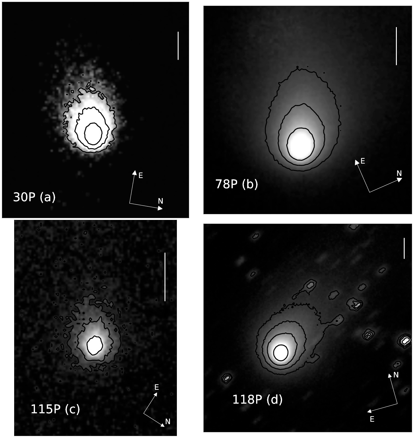
Figure 1: Observations obtained using a CCD camera at 1.52 m telescope of the Observatorio de Sierra Nevada in Granada, Spain. (a) 30P/Reinmuth 1 on May 15, 2010. Isophote levels in Solar Disk Units (SDU) are 2.00$\times{10^{-13}}$, 0.75$\times{10^{-13}}$, and 0.25$\times{10^{-13}}$. (b) 78P/Gehrels 2 on December 19, 2011. Isophote levels are 0.55$\times{10^{-12}}$, 2.65$\times{10^{-13}}$, and 1.35$\times{10^{-13}}$. (c) 115P/Maury on July 15, 2011. Isophote levels are 1.00$\times{10^{-13}}$, 3.00$\times{10^{-14}}$, and 1.30$\times{10^{-14}}$. (d) 118P/Shoemaker-Levy 4 on December 12, 2009. Isophote levels are 1.50$\times{10^{-13}}$, 6.00$\times{10^{-14}}$, 3.50$\times{10^{-14}}$, and 2.00$\times{10^{-14}}$. In all cases, the directions of celestial North and East are given. The vertical bars correspond to 10⁴km in the sky.

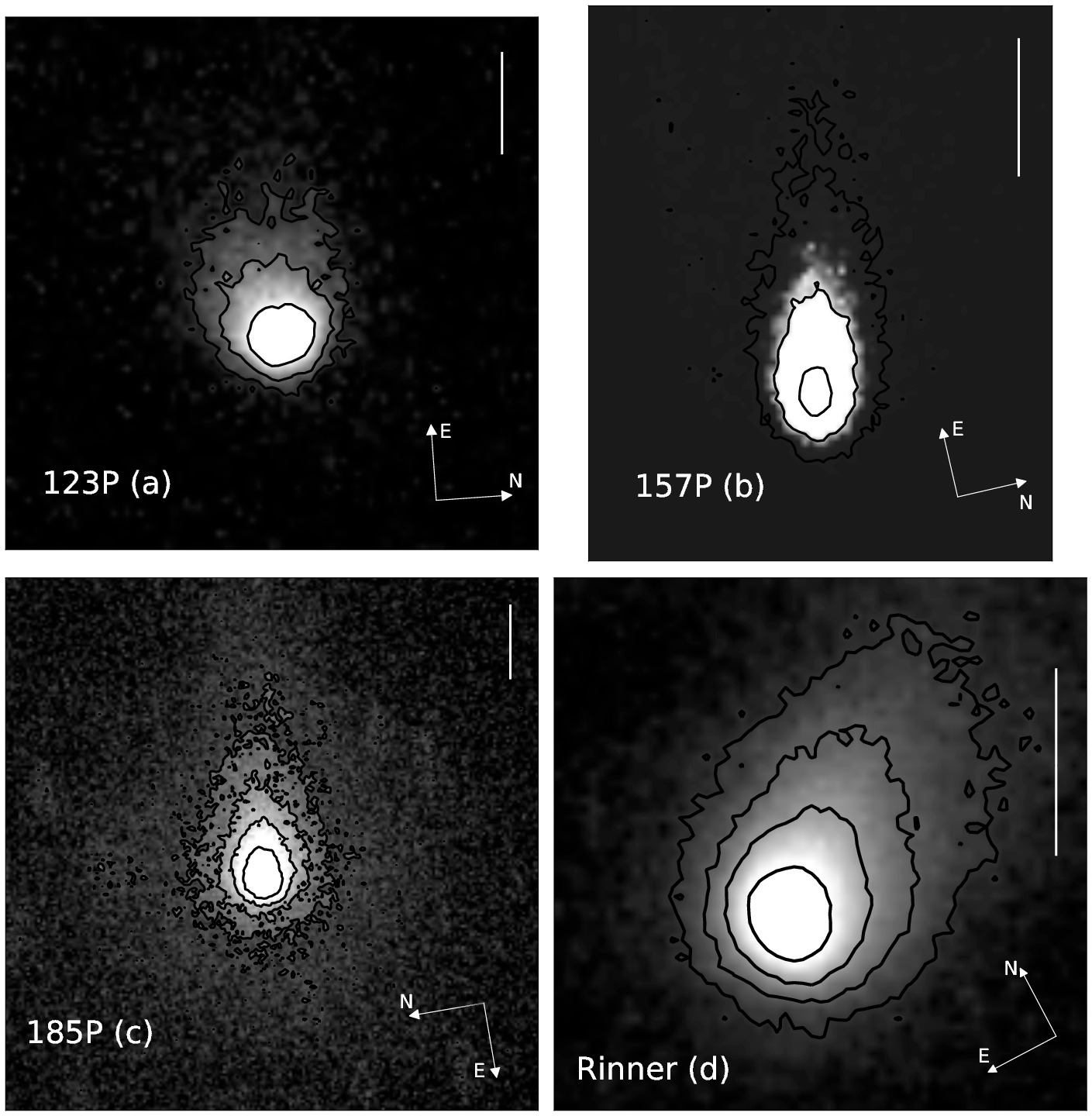
Figure 2: Observations obtained using a CCD camera at 1.52 m telescope of the Observatorio de Sierra Nevada in Granada, Spain. (a) 123P/West-Hartley on February 26, 2011. Isophote levels in Solar Disk Units (SDU) are 1.00$\times{10^{-13}}$, 0.35$\times{10^{-13}}$, and 0.15$\times{10^{-13}}$. (b) 157P/Tritton on March 10, 2010. Isophote levels are 6.00$\times{10^{-13}}$, 0.75$\times{10^{-13}}$, and 2.65$\times{10^{-14}}$. (c) 185P/Petriew on July 15, 2012. Isophote levels are 1.80$\times{10^{-13}}$, 1.00$\times{10^{-13}}$, 0.60$\times{10^{-13}}$, and 0.35$\times{10^{-13}}$. (d) P/2011 W2 (Rinner) on January 4, 2012. Isophote levels are 6.00$\times{10^{-14}}$, 2.70$\times{10^{-14}}$, 1.50$\times{10^{-14}}$, and 0.80$\times{10^{-14}}$. In all cases, the directions of celestial North and East are given. The vertical bars correspond to 10⁴km in the sky.

The first block of our observation data were taken at the 1.52 m telescope of Sierra Nevada Observatory (OSN) in Granada, Spain. We used a 1024$\times$1024 pixel CCD camera with a Johnson red filter to minimize gaseous emissions. The pixel size in the sky was 0.”46, so the field of view was 7’.8$\times$7’.8. To improve the signal-to-noise ratio, the comets were imaged several times using integration times in the range 60-300 sec. The individual images at each night were bias subtracted and flat-fielded using standard techniques. The flux calibration was made using the USNO-B1.0 star catalog (Monet et al., 2003).The individual images of the comets were calibrated to mag arcsec^-2 and then converted to solar disk intensity units (hereafter SDU). After calibration, the images corresponding to each single night were shifted to a reference image by taking their apparent sky motion into account, and then a median of those images was taken. For the modeling purposes, the final images are rotated to the photographic plane $(N,M)$ (Finson & Probstein, 1968), where the Sun is toward $-M$. Table 2 shows the log of the observations. Negative values in time to perihelion correspond to pre-perihelion observations. Representative images are displayed in Figs. 1 and 2.

The second block of observational data correspond to the $Af\rho$ curves around perihelion date ($\sim{300}$ days). These observations were carried out by the amateur astronomical association Cometas-Obs. The $Af\rho$ measurements are presented as a function of the heliocentric distance and are always referred to an aperture of radius $\rho=10^{4}$ km projected on the sky at each observation date. The calibration of the Cometas-Obs observations was performed with the star catalogs CMC-14 and USNO A2.0.

Table 2: Log of the OSN observations.

Comet	Observation Date	$r_{h}$ 1	$\Delta$	Resolution	Phase	Position	$Af\rho$ ($\rho=10^{4}km$) 2
	(UT)	(AU)	(AU)	(km pixel-1)	Angle (∘)	Angle (∘)	(cm)
30P/Reinmuth 1	2010 Mar 10 21:45	-1.916	1.579	526.8	31.1	87.1	52
	2010 May 15 21:10	1.898	2.147	716.3	28.0	99.6	61
78P/Gehrels 2	2011 Dic 19 20:00	-2.018	1.647	549.5	28.9	66.5	380
	2012 Jan 4 20:15	-2.009	1.805	602.2	29.2	67.0	470
115P/Maury	2011 Jul 2 22:00	-2.146	1.343	448.0	18.5	122.7	17
118P/Shoemaker-Levy 4	2009 Dec 12 01:45	-1.991	1.032	1377.2	8.9	324.9	103
123P/West-Hartley	2011 Feb 26 23:00	-2.346	1.970	657.3	24.5	86.4	40
	2011 Mar 31 21:00	2.253	2.252	751.3	25.6	85.4	50
157P/Tritton	2010 Mar 10 21:30	1.376	1.343	448.0	42.8	77.0	20
185P/Petriew	2012 Jul 15 03:15	-1.027	1.097	366.0	57.0	260.2	17
P/2011 W2 (Rinner)	2011 Dic 22 03:00	2.326	1.451	484.1	14.0	309.9	18
	2012 Jan 4 02:00	2.340	1.412	471.2	10.2	332.2	22

3 Monte Carlo dust tail model

The dust tail analysis was performed by the Monte Carlo dust tail code, which allows us to fit the OSN images and the observational $Af\rho$ curves provided by Cometas-Obs. This code has been successfully used on previous works on characterization of dust environments of comets and Main-belt comets, such as 29P/Schwassmann-Wachmann 1 and P/2010 R2 (La Sagra) (Moreno, 2009; Moreno et al., 2011). This code is also called the Granada model (see Fulle et al., 2010) in the dust studies for the Rosetta mission target, 67P/Churyumov-Gerasimenko. The model describes the motion of the particles when they leave the nucleus and are submitted to the gravity force of the Sun and the radiation pressure, so that the trajectory of the particles around the Sun is Keplerian. The $\beta$ parameter is defined as the ratio of the radiation pressure force to the gravity force and is given for spherical particles as $\beta=C_{pr}Q_{pr}/(\rho_{d}d)$, where $C_{pr}=1.19\times 10^{-3}$ km m^-2; $Q_{pr}$ is the scattering efficiency for radiation pressure, which is $Q_{pr}\sim 1$ for large absorbing grains (Burns et al., 1979); $\rho_{d}$ is the mass density, assumed at $\rho_{d}=10^{3}$ kg m^-3; and $d$ is the particle diameter. We use Mie theory for the interaction of the electromagnetic field with the spherical particles to compute the geometric albedo, $p_{v}$, and $Q_{pr}$. The parameter, $p_{v}$, is a function of the phase angle $\alpha$ and the particle radius. We assume the particles as glassy carbon spheres of refractive index $m=1.88+0.71i$ (Edoh, 1983) at $\lambda=0.6$ $\mu$m. We compute a large number of dust particle trayectories and calculate their positions on the $(N,M)$ plane and their contribution to the tail brightness. The free parameters of the model are dust mass loss rate, the ejection velocities of the particles, the size distribution, and the dust ejection pattern.

3.1 $Af\rho$

The $Af\rho$ quantity [cm] (A’Hearn et al., 1984) is related to the dust coma brightness, where $A$ is the dust geometric albedo, $f$ the filling factor in the aperture field of view (proportional to the dust optical thickness), and $\rho$ is the linear radius of aperture at the comet, which is the sky-plane radius. When the cometary coma is in steady-state, $Af\rho$ is independent of the observation coma radius $\rho$ if the surface brightness of the dust coma is proportional to $\rho^{-1}$. It is formulated as follows:

$$Af\rho={4r_{h}^{2}\Delta^{2}\over\rho}\frac{F_{c}}{F_{s}}\;,$$ (1)

where $r_{h}$ is the heliocentric distance and $\Delta$ the geocentric distance. The parameter, $F_{c}$, is the measured cometary flux integrated within a radius of aperture $\rho$, and $F_{s}$ is the total solar flux. For each comet, we have the $Af\rho$ curve as heliocentric distance function provided by Cometas-Obs for an aperture of radius $\rho=10^{4}$ km, $\sim 300$ days around perihelion, and the $Af\rho$ measurements derived from the OSN observations with the same aperture. Some of the $Af\rho$ data correspond to times, where the phase angle was close to zero degree, so that the backscattering enhancement became apparent (Kolokolova et al., 2004). We could not model this enhancement: for the assumed absorbing spherical particles, the phase function is approximately constant except for the forward spike for particles whose radius is r$\geq\lambda$. Then, we corrected these enlarged $Af\rho$ at small phase angles by assuming a certain linear phase coefficient, which we apply to the data at phase angles $\alpha\leq 30^{\circ}$. We adopted a linear phase coefficient of 0.03 mag $deg^{-1}$, which is in the range 0.02-0.04 mag $deg^{-1}$ estimated by Meech & Jewitt (1987) from various comets. In this way, the corrected $Af\rho^{\prime}$ values are computed as a function of the original $Af\rho$ values at phase angle $\alpha$ as:

$$Af\rho^{\prime}=10^{\frac{-\beta(30-\alpha)}{2.5}}Af\rho\;.$$ (2)

To illustrate this correction, we show in its application to comet 78P/Gehrels 2 Fig. 3. In the upper panel, the correlation of the original $Af\rho$ data with the phase angle and the lower panel the final $Af\rho$ curve after correcting those values by equation (2) is seen. The same equation is applied to the OSN images when the phase angle is $\alpha\leq 30^{\circ}$ (see table 2).

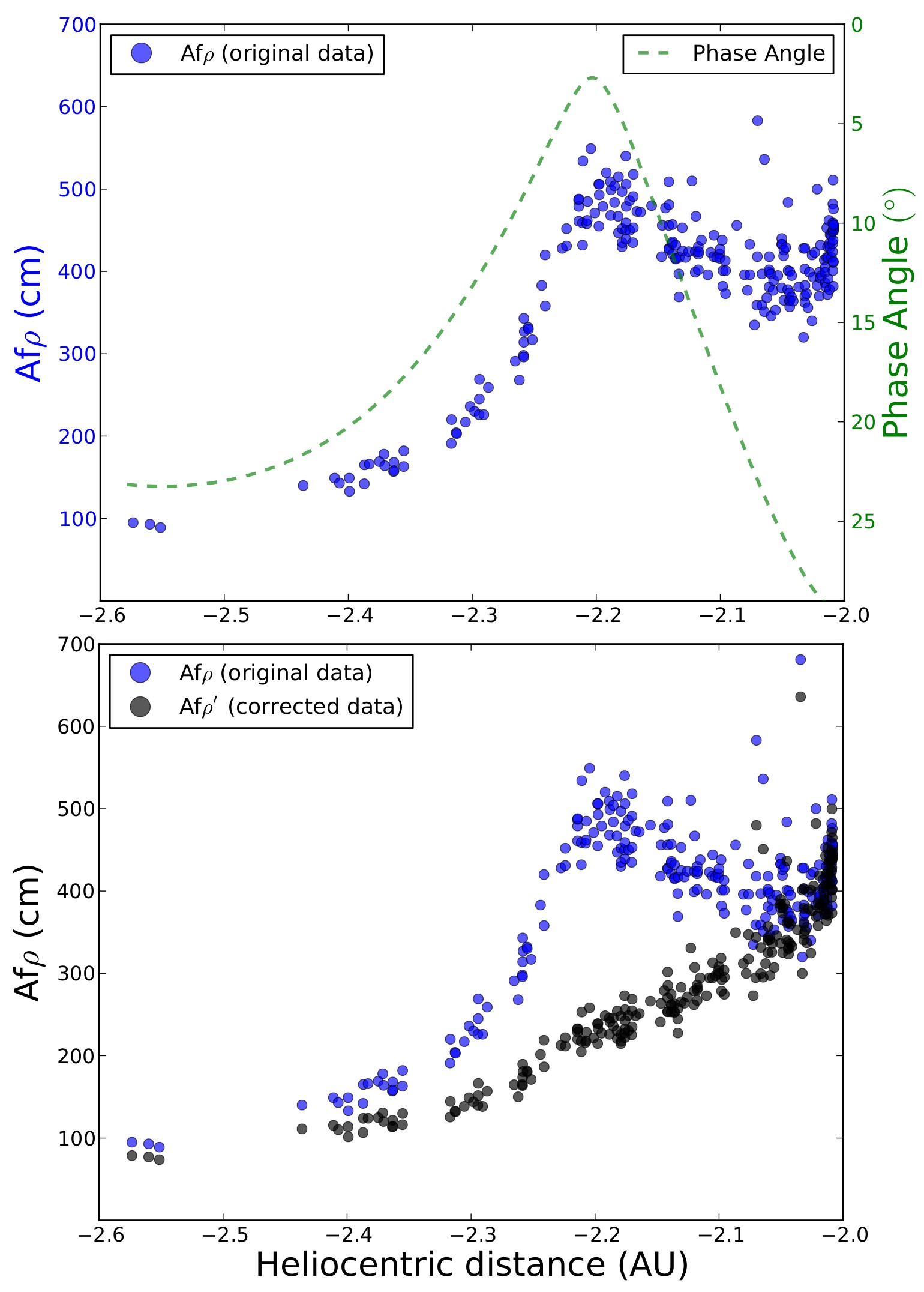
Figure 3: $Af\rho$ pre-perihelion measurements of comet 78P/Gehrels 2 provided by Cometas-Obs. Upper panel: original $Af\rho$ measurements and phase angle as a function of heliocentric distance. Lower panel: $Af\rho$ and $Af\rho^{\prime}$ after the backscattering effect correction using equation (2) as function of heliocentric distance.

4 Dust analysis

As described in the previous section, we use our Monte Carlo dust tail code to retrieve the dust properties of each comet in our sample. The code has many important parameters, so that a number of simplifying assumptions should be made to make the problem tractable. The dust particles are assumed spherical with a density of 1000 kg m^-3 and a refractive index of $m=1.88+0.71i$, which is typical of carbonaceous spheres at red wavelengths (Edoh, 1983). This gives a geometric albedo of $p_{v}=0.04$ for particle sizes of r$\gtrsim 1\mu m$ at a wide range of phase angles. The particle ejection velocity is parametrized as $v(t,\beta)=v_{1}(t)\times\beta^{1/2}$, where $v_{1}(t)$ is a time dependent function to be determined in the modeling procedure. In addition, the emission pattern, which are possible spatial asymmetries in the particle ejection, might appear. The asymmetric ejection pattern is parametrized by considering a rotating nucleus with active areas on it, whose rotating axis is defined by the obliquity, $I$, and the argument of the subsolar meridian at perihelion, as defined in Sekanina (1981). The rotation period, $P$, is not generally constrained if the ejecta age is much longer than $P$, which is normally the case. The particles are assumed distributed broadly in size, so that the minimum size is always set in principle in the sub-micrometer range, while the maximum size is set in the centimetre range. The size distribution is assumed to be given by a power law, $n(r)\propto r^{-\delta}$, where $\delta$ is set to vary in the -4.2 to -3 domain, which is the range that has been determined for other comets (e.g., Jockers, 1997). All of those parameters, $v_{1}(t)$, $r_{min}$, $r_{max}$, and $\delta$, and the mass loss rate are a function of the heliocentric distance, so that some kind of dependence on $r_{h}$ must be established. In addition, the activity onset time should also be specified. On the other hand, current knowledge of physical properties of cometary nuclei established the bulk density below $\rho=1000$ kg m^-3 (Carry, 2012). Values of $\rho=600$ kg m^-3 have been reported for comets 81P/Wild 2 (Davidsson & Gutierrez, 2004) and Temple 1 (A’Hearn et al., 2005), so we adopted that value. The ejection velocity at a distance R$\sim 20R_{N}$, where R_N is the nucleus radii and R is the distance where the gas drag vanishes, should overcome the escape velocity, which is given by $v_{esc}=\sqrt{2GM/R}$. Assuming a spherically-shaped nucleus, we get $v_{esc}=R_{N}\sqrt{(2/15)\pi\rho G}$, where $\rho=600$ kg m^-3. In cases where $R_{N}$ has been estimated by other authors, the minimum ejection velocity should verify the condition $v_{min}\gtrsim v_{esc}$. Considering that the minimum particle velocity determined in the model is $v_{min}\sim v_{esc}$, we can give an upper limit estimate of the nucleus radius in all the other cases.

The Monte Carlo dust tail code, is a forward code whose output is a dust tail image corresponding to a given set of input parameters. Given the large amount of parameters, the solution is likely not unique: approximately the same tail brightness can be likely achieved by assuming another set of input parameters. However, if the number of available images and/or $Af\rho$ measurements cover a significant orbital arc, it is clear that the indetermination is reduced. Our general procedure first consists in assuming the most simple case: isotropic particle ejection, $r_{min}=1\mu$m, $r_{max}=1$cm, $v_{1}(t)$ monotonically increasing toward perihelion, $\delta=-3.5$, and $dM/dt$ set to a value, which reproduce the measured tail intensity in the optocenter, assuming a monotonic decrease with heliocentric distance. From this starting point, we then start to vary the parameters, assuming a certain different dependence with heliocentric distance, until an acceptable agreement with both the dust tail images and the $Af\rho$ measurements is reached. Then, if we find no way to fit the data using an isotropic ejection model after many trial-and-error procedures, we switch to the anisotropic model where the active area location and rotational parameters must be set.

Using the procedure described above for each comet in the sample, we present the results on the dust parameters organized in the following way: in tabular form, where the main properties derived of the dust environment of each comet is given (tables 3 and 4), and a series of plots on the dependence on the heliocentric distance of the dust mass loss rate, the ejection velocities for $r=1$ cm particles, the maximum particle size, and the power index of the size distribution. Representative plot is shown in the case of the comet 30P in Fig. 4 and in appendix B, the results for each comet are individually displayed (see figures 12 to 18). In addition, the representative plot of the comparison between observations and model in the case of the comet 30P is shown in Fig. 5, and the comparison between observations and models for each comet individually are displayed in the appendix C (figures 19 to 25).

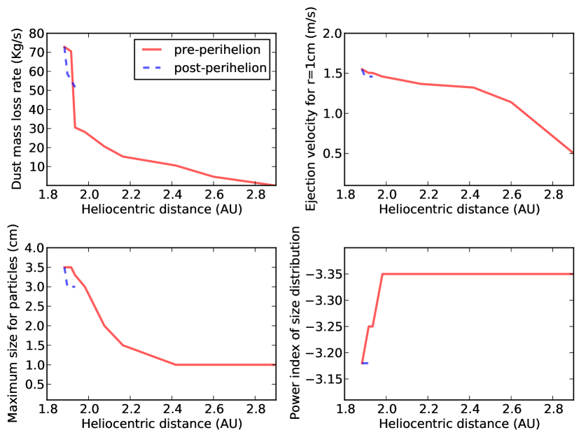
Figure 4: Representative figure of the evolution of the dust parameter evolution obtained in the model versus the heliocentric distance for comet 30P/Reinmuth 1. The panels are as follows: (a) dust mass loss rate [kg/s]; (b) ejection velocities for particles of r=1 cm glassy carbon spheres [m/s]; (c) maximum size of the particles [cm]; and (d) power index of the size distribution. In all cases, the solid red lines correspond to pre-perihelion and the dashed blue lines to post-perihelion. In appendix B, the results for each comet individually are displayed (see figures 12 to 18).

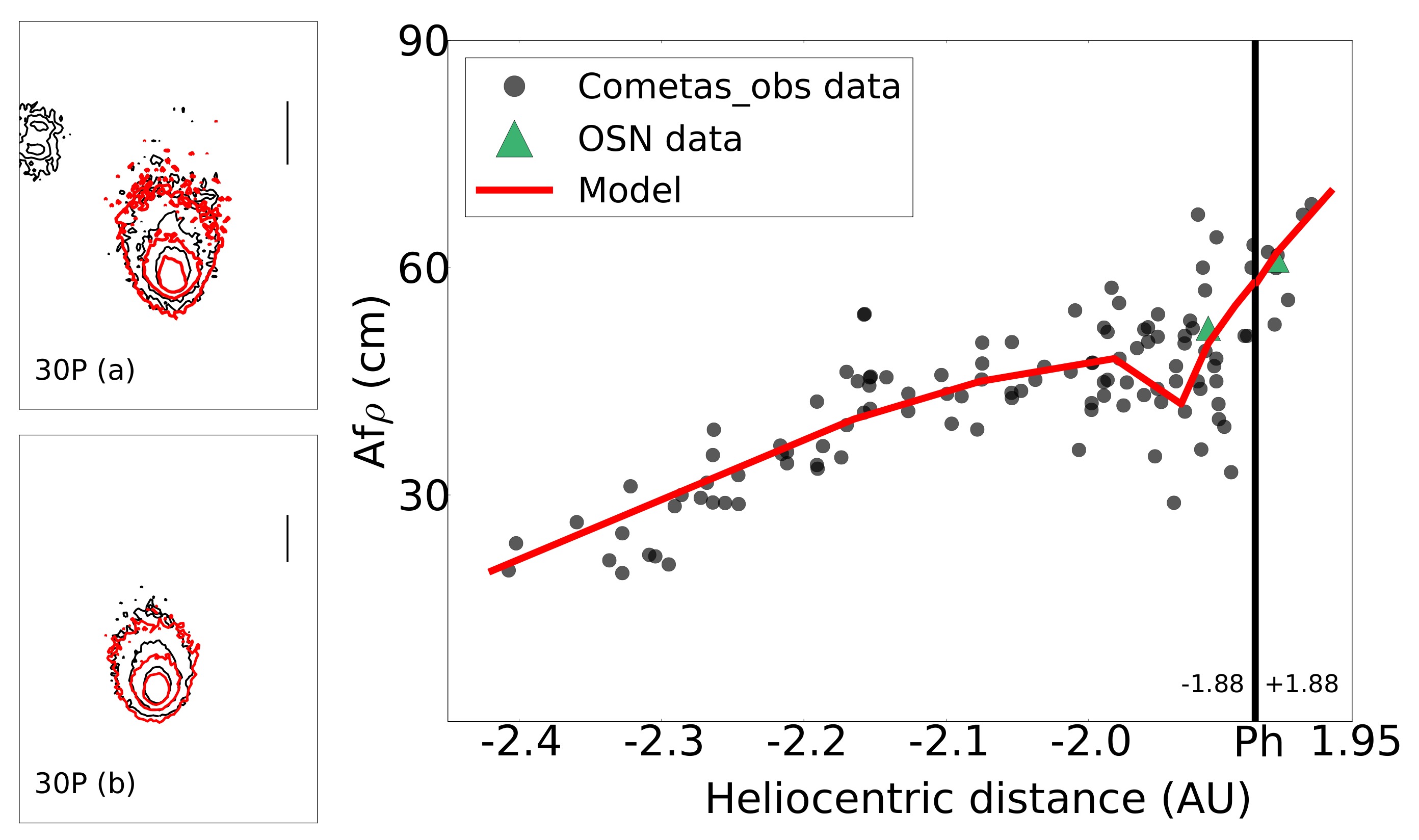
Figure 5: Representative figure of the comparison between observations and model of comet 30P/Reinmuth 1. Left panels: isophote fields (a) March 10, 2010, and (b) May 15, 2010. In both cases, isophote levels are 2.00$\times{10^{-13}}$, 0.75$\times{10^{-13}}$, and 0.25$\times{10^{-13}}$ SDU. The black contours correspond to the OSN observations and the red contours to the model. Vertical bars correspond to $10^{4}$ km on the sky. Right panel: parameter $Af\rho$ versus heliocentric distance. The black dots correspond to Cometas-Obs data, and the green triangles are the OSN data, which correspond to March 10 and May 15, 2010. The red line is the model. The observations and the model refer to $\rho=10^{4}$km. In appendix C, the comparison between observations and models for each comet individually are displayed (see figures 19 to 25).

4.1 Discussion

The dust environment of the 22P was already reported by Moreno et al. (2012), where the authors concluded that this comet shows a clear time dependent asymmetric ejection behavior with an enhanced activity at heliocentric distances beyond 2.5 AU pre-perihelion. This is also accompanied by enhanced particle ejection velocity. The maximum size for the particles were estimated as 1.4 cm with a constant power index of -3.1. The peak of dust mass loss rate and the peak of ejection velocities were reached at perihelion with values $Q_{d}=260$ kg s^-1 and $v=2.7$ m s^-1 for 1-cm grains. The total dust lost per orbit was $8\times 10^{9}$ kg. The annual dust loss rate is $T_{d}=1.24\times 10^{9}$ kg yr^-1 , and the averaged dust mass loss rate per orbit is 40 kg/s. The contribution to the interplanetary dust of this comet corresponds to about 0.4$\%$ of the $\sim 2.9\times 10^{11}$ kg yr^-1 that must be replenished if the cloud of interplanetary dust is in steady state (Grun et al., 1985).

For 30P, 115P, and 157P, we derived an anisotropic ejection pattern with active areas on the nucleus surface (see table 3). In the case of 30P, the rotational parameters, $I$ and $\phi$, have been taken from Krolikowska et al. (1998) as $I=107^{\circ}$ and $\phi=321^{\circ}$. However, for 115P and 157P, these parameters have been derived from the model. The 78P is the most active comet in our sample with a peak dust loss rate at perihelion with a value of $Q_{d}=530$ kg s^-1 and a total dust mass ejected of $5.8\times 10^{9}$ kg. This comet was study by Mazzotta Epifani & Palumbo (2011) in its previous perihelion passage on October 2004. The authors estimated that the dust production rate at perihelion with values between $Q_{d}=14-345$ kg s^-1 using a method derived from the one used by Jewitt (2009) to compute the dust production rate of active Centarus. They also obtained $Af\rho=846\pm 55$ cm in an aperture of radius $\rho=7.3\times 10^{3}$ km, and they concluded that this comet is more active than the the average Jupiter Family Comets at a given heliocentric distance. In addition, Lowry & Weissman (2003) reported a stellar appearance of 78P at $r_{h}=5.46$ AU pre-perihelion, and any possible coma contribution to the observed flux was likely to be small or non existent, which is consistent with our model where the comet is not active at such large pre-perihelion distances. From our studies, we can classify our targets in three different categories: weakly active comets (115P, 157P, and Rinner) with an average annual dust production rate of $T_{d}<1\times 10^{8}$ kg yr^-1; moderately active comets (30P, 123P, and 185P) with $T_{d}=1-3\times 10^{8}$ kg yr^-1; and highly active comets (22P, 78P, and 118P) with $T_{d}>8\times 10^{8}$ kg yr^-1. It is necessary to consider that we do not have observations after perihelion for the comet 115P and 123P. That is, our observational information covers less than half of the orbit, losing the part of the branch which is supposed to be the most active. For this reason, our results for these comets are lower limits in the $T_{d}$ measurements.

Table 3: Dust properties summary of the targets under study I.

Comet	Emission	Active areas	Size distribution	Size distribution	Maximum nucleus	Obliquity	Argument of subsolar
	pattern 1	location (∘)	$r_{min},r_{max}$ (cm)	$\delta_{min},\delta_{max}$	radius (km)	(∘)	meridan at perihelion (∘)
30P/Reinmuth 1	Ani (50%)	-30 to +30	10-4, 3.5	-3.35, -3.18	3.9 2	107 3	133 3
78P/Gehrels 2	Iso (100%)	–	10-4, 3.0	-3.40, -3.05	3.6	–	–
115P/Maury	Ani (70%)	-20 to +60	10-4, 4.0	-3.13, -3.05	4.0	25	280
118P/Shoemaker-Levy 4	Iso (100%)	–	10-4, 3.0	-3.20, -3.05	2.4 4	–	–
123P/West-Hartley	Iso (100%)	–	10-4, 2.5	-3.32, -3.15	2.0 5	–	–
157P/Tritton	Ani (70%)	-30 to +30	10-4, 3.0	-3.35, -3.15	1.6	10	150
185P/Petriew	Iso (100%)	–	10-4, 6.0	-3.60, -3.00	5.7	–	–
P/2011 W2 (Rinner)	Iso (100%)	–	10-4, 2.5	-3.20, -3.15	2.2	–	–

Table 4: Dust properties summary of the targets under study II.

Comet	Peak dust loss	Peak ejection velocity	Total dust mass	Total dust mass	Averaged dust	Contribution to the
	rate (kg/s)	of 1-cm grains (m/s)	ejected (kg)	ejected per year (kg/yr)	mass loss rate (kg/s)	interplanetary dust (%) 1
30P/Reinmuth 1	73.0	1.4	$8.2\times 10^{8}$	$2.1\times 10^{8}$	6.8	0.07
78P/Gehrels 2	530.0	2.1	$5.8\times 10^{9}$	$1.5\times 10^{9}$	47.5	0.52
115P/Maury	45.0	1.4	$2.9\times 10^{8}$	$6.9\times 10^{7}$	2.1	0.02
118P/Shoemaker-Levy 4	180.0	2.3	$2.3\times 10^{9}$	$6.5\times 10^{8}$	20.8	0.22
123P/West-Hartley	65.0	1.8	$5.4\times 10^{8}$	$1.4\times 10^{8}$	4.5	0.05
157P/Tritton	50.0	2.1	$2.9\times 10^{8}$	$8.7\times 10^{7}$	2.7	0.03
185P/Petriew	143.0	7.2	$9.0\times 10^{8}$	$3.0\times 10^{8}$	9.6	0.10
P/2011 W2 (Rinner)	15.0	1.7	$2.6\times 10^{8}$	$6.4\times 10^{7}$	2.0	0.02

5 Dynamical history analysis

Levison & Duncan (1994) were the first to make a comprehensive set of long-term integrations (up to $10^{7}$ yr) to study the dynamical evolution of short period comets. The authors argue that it is necessary to make a statistical study using several orbits for each comet with slightly different initial orbital elements due to the chaotic nature of each individual orbit. For this reason, the authors made a 10 Myr backward (and forward) integration for the 160 short period comets know at that time and 3 clones for each comet with offsets in the positions along the $x$, $y$, and $z$ directions of +0.01 AU. That is, they used 640 test particles for their integrations. They conclude that the long-term integrations into the the past or future are statistically equivalent, and they obtained that $\sim 92\%$ of the total particles were ejected from the Solar System, and $\sim 6\%$ were destroyed by becoming Sun-grazers. The median lifetime of Jupiter Family Comets (hereafter JFCs) was derived as $3.25\times 10^{5}$ yr. In a later study of the same authors (Levison & Duncan, 1997), they estimated that the physical lifetime of JFCs is between (3-25)$\times 10^{3}$ yr, where the most likely value is 12$\times 10^{3}$ yr. In our case, we use the Mercury package version 6.2, a numerical integrator developed by Chambers (1999), to determine the dynamical evolution of our targets, that has been used by other authors with the same purpose (e.g., Hsieh et al., 2012a, b; Lacerda, 2013). Due to the chaotic nature of the targets, which was mentioned in the Levison & Duncan (1994) study, we generate a total of 99 clones having 2$\sigma$ dispersion in three of the orbital elements: semimajor axis, eccentricity, and inclination (hereafter $a$, $e$, and $i$), where $\sigma$ is the uncertainty in the corresponding parameter as given in the JPL Horizons on-line Solar System data (see ssd.pjl.nasa.gov/?horizons). In table 5, we show the orbital parameters and the $1\sigma$ uncertainty of our targets extracted from that web page. These 99 clones plus the real object make a total of 100 massless test particles to perform a statistical study for each comet, which supposes 900 massless test particles. The Sun and the eight planets are considered as massive bodies. We used the hybrid algorithm, which combines a second-order mixed-variable symplectic algorithm with a Burlisch-Stoer integrator to control close encounters. The initial time step is 8 days, and the clones are removed any time during the integration when they are beyond 1000 AU from the Sun. The total integration time was 15 Myr, which is time enough to determine the most visited regions for each comet and derive the time spent in the region of JFCs, region that is supposed to be the location where the comets reach a temperature high enough to be active periodically. We divide the possible locations of the comets in four regions attending to their dynamical properties at each moment in the study: JFCs-type with $a<a_{S}/(1+e)$; Centaur-type, confined by $a_{S}/(1+e)<a<a_{N}$ and $e<0.8$; Halley-type, which is similar to Centaur-type but with $e>0.8$; and Transneptunian-type with $a>a_{N}$, where $a_{S}$ and $a_{N}$ are the semimajor axes of Saturn and Neptune, respectively.

In this study, we neglect the non-gravitational forces using the same arguments as Lacerda (2013). Thus, assuming that the non-gravitational acceleration, $T$, is due to a single sublimation jet tangential to the comet orbit, the change rate of the semimajor axis is described by

$$da/dt=2Va^{2}T/GM_{\odot}\;,$$ (3)

where $T$ is the acceleration due to the single jet and is given by

$$T=(dM_{d}/dt)(v_{d}/m_{nuc})\;.$$ (4)

In these equations, $V$ is the orbital velocity, $a$ is the semimajor axis, $G$ is the gravitational constant, $M_{\odot}$ is the Sun mass, $v_{d}$ is the dust velocity, and $m_{nuc}$ is the mass of the nucleus. To show a general justification to neglect the gravitational forces that are valid to our complete list of targets, we compute the maximum rate of change of the semimajor axis that corresponds to the comet using the maximum $a$, maximum $dM/dt$, maximum $v_{d}$, and minimum $m_{nuc}$. From our comet sample, these values are $a_{max}=4.25$ AU (115P), $(dM/dt)_{max}=47.5$ kg s^-1 (78P), $(v_{d})_{max}=708$ m s^-1 (185P). The minimum comet nucleus was inferred for 157P as $R_{N}\leq 1.6$ km, so we adopt $(R_{N})_{min}=1.6$ km, which is a minimum nucleus of $(m_{nuc})_{min}=1.03\times 10^{13}$ kg. Taken all those values together, we get $T=2.2\times 10^{-5}$ AU yr^-2 and $da/dt=4.8\times 10^{-5}$ AU yr^-1. On the other hand, the lifetime of sublimation from a single jet would be $t_{sub}=6871$ yr, which is based on the nucleus size and $(dM/dt)_{max}$. Then, the total deviation in semimajor axis would be $(da/dt)_{max}\times t_{sub}=0.33$ AU. This deviation, which should be considered as an upper limit, is completely negligible in the scale of variations we are dealing with in the dynamical analysis of the orbital evolution. This result is close to the one derived for Lacerda (2013), where the author gives the maximum semimajor deviation for P/2010 T020 LINEAR-Grauer as 0.42 AU.

As a result of our 15 Myr backward integration for all targets, we find that the $\sim 98\%$ of the particles are ejected before the end of the integration, and in almost all cases, the surviving clones are in the transneptunian region. Thus, we focused on the first 1 Myr of backward in the orbital evolution, where the $\sim 20\%$ of the test particles still remain in the Solar System. This time is enough to obtain a general view of the visited regions by each comet. After that, we display the last 5000 yr with a 100 yr temporal resolution to obtain the time spent by these comets in the JFCs region with a confidence level of $90\%$.

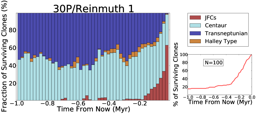
Figure 6: 30P/Reinmuth 1 backward in time orbital evolution during 1 Myr. Left panel: fraction of surviving clones ($\%$) versus time from now (Myr). The colors represent the regions visited by the test particles (red: Jupiter Family region; cyan: Centaur; blue: Transneptunian; yellow: Halley Type). The resolution is $2\times 10^{4}$ yr. Right bottom panel: the $\%$ of surviving clones versus time from now (Myr), where N=100 is the number of the initial test massless particles.

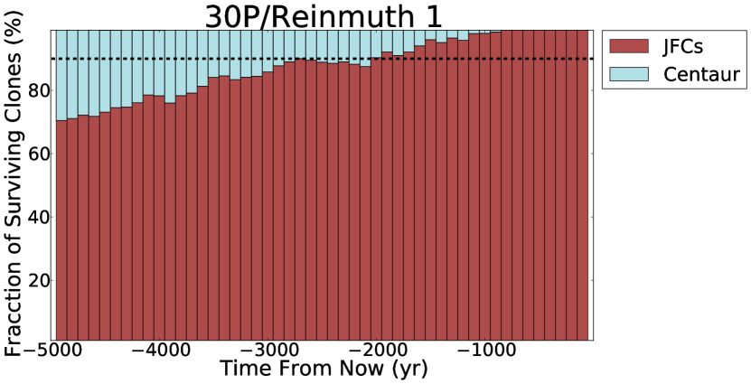
Figure 7: 30P/Reinmuth 1 during the last $5\times 10^{3}yr$. Fraction of surviving clones ($\%$) versus time from now (Myr). The colors represent the regions visited by the test particles (red: Jupiter Family region; cyan: Centaur). The dashed line marks the bars with a confidence level equal or larger than 90$\%$ of the clones in the Jupiter Family region. The resolution is 100 yr, and the number of the initial test particles is N=100.

As an example of this procedure, we show the results for 30P (see Fig. 6) in detail. For this comet, we determined that $85\%$ of the particles were ejected from the Solar System after 1 Myr of backward integration. We can see that most of the particles stay in the JFCs region during the first $\sim 2\times 10^{4}$ yr , but they moved on into further regions as centaurs and transneptunian objects at $\sim 2\times 10^{5}$ yr. To determine the time spent by 30P in the JFCs region, we show the last $5\times 10^{3}$ yr with a resolution of 100 yr in Fig. 7. We derive with 90$\%$ of confidence level that 30P comet spent $\sim 2\times 10^{3}$ yr in this location.

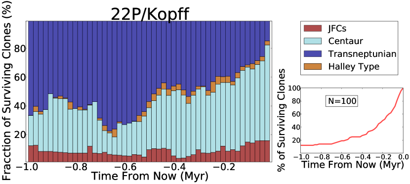
Figure 8: As in Fig. 6, but for comet 22P/Kopff.

Figure 9: As in Fig. 7, but for comet 22P/Kopff.

A special case within the sample is comet 22P, which turned to be the youngest one in our study. Its dynamical analysis shows that the $88\%$ of the test particles are ejected from the Solar System before 1 Myr. The probability to be at the JFCs region in this period remains always under 20$\%$ (Fig. 8). If we focused on the last $5\times 10^{3}$ yr (see Fig. 9), we determine the time spent in JFCs region as $\sim 100$ yr. This agrees with its discovery in 1906. It seems that this comet came from the Centaur region, which is the most likely region occupied by the object along this period.

5.1 Discussion

From the dynamical analysis, we determine that, just 12 of the initial 900 particles (9 real comets + 99 clones per each one) survived after a 15 Myr backward integration, which means 1.3$\%$. This result agrees with Levison & Duncan (1994), who concluded that just 11$\pm 4$ particles, or $1.5\pm 0.6\%$, remained in the Solar System after integration from their dynamical study. In Fig. 10, we show the surviving clones in the $a$-$e$ plane, where just one of the clones is in the Centaur region (118P/clon74) and the rest of them are in the transneptunian region. Two of the clones have $a>100$ AU with a very high eccentricity ($e>0.9$), 30P/clon91 and Rinner/clon31. On the other hand, there are two comets with low eccentricity, 78P/clon86 and 118P/clon13, with $e<0.25$. The rest of the surviving clones have intermediate values of eccentricity, $0.45<e<0.8$, and it seems that these comets are in a transition state between Kuiper Belt and the Scattered Disk objects (Levison & Duncan, 1997).

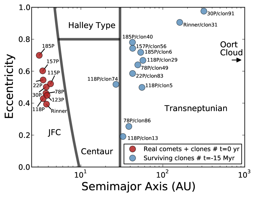
Figure 10: Time evolution of the 900 initial particles in the 15 Myr backward integration. Red circles are the real comets and their clones (in the same location for t=0 yr, which is current position, just 2$\sigma$ dispersion in the orbital parameters), and the blue circles are the surving particles after 15 Myr.

In addition, we derived the time spent by all the comets under study in the JFCs region with a 90$\%$ of confidence level. We can see that the youngest is 22P, followed by 78P, and 118P ($\sim 100$,$\sim 500$, and $\sim 600$ yr respectively). On the other hand, the oldest comet in our sample is 123P with $\sim 3.9\times 10^{3}$ yr. This result is shown in Fig. 11, where we relate the annual dust production rate ($T_{d}$, see section 4) within the time spent in the JFCs region for each comet. It seems that the most active comets in our sample are at the same time the youngest ones, which are, 22P, 78P and 118P.

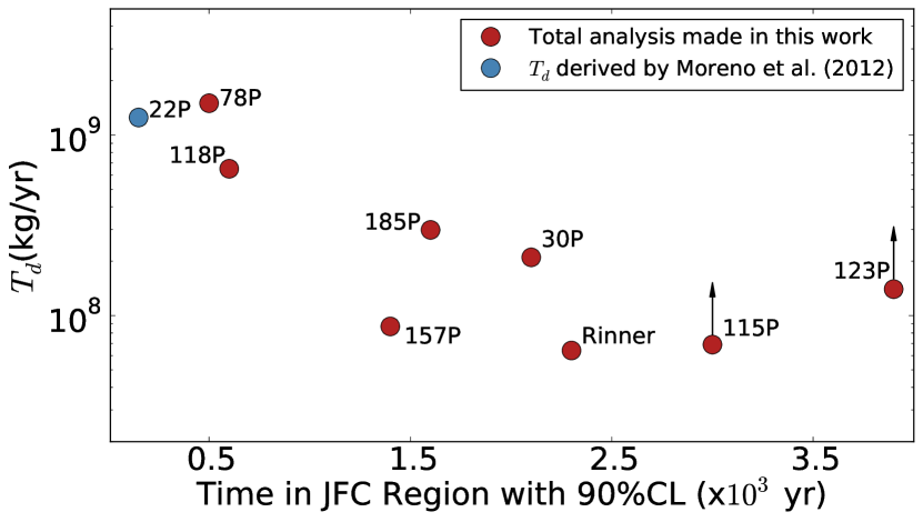
Figure 11: Annual dust production rate of our targets obtained in the dust analysis (see section 4) versus the time in the JFCs region with a $90\%$CL derived in dynamical studies (see section 5). The comets with arrows mean the $T_{d}$ given for them are lower limits.

6 Summary and conclusions

We presented optical observations, which were carried out at Sierra Nevada Observatory on 1.52 m telescope, of eight JFCs comets during their last perihelion passage: 30P/Reinmuth 1, 78P/Gehrels 2, 115P/Maury, 118P/Shoemaker-Levy 4, 123P/West-Hartley, 157P/Tritton, 185/Petriew, and P/2011 W2 (Rinner). We also benefited from $Af\rho$ curves of these targets along $\sim{300}$ days around perihelion, which is provided by Cometas-Obs. We used our Monte Carlo dust tail code (e.g. Moreno, 2009) to derive the dust properties of our targets. These properties were dust loss rate, ejection velocities of particles, and size distribution of particles, where we gave the minimum and maximum size of particles and the power index of the size distribution $\delta$. We also obtained the overall emission pattern for each comet, which could be either isotropic or anisotropic. When the ejection was derived as anisotropic, we could estimate the location of the active areas on the surface and the rotational parameters given by $\phi$ and $I$. From this analysis, we have determined three categories according to the amount of dust emitted:

1. Weakly active: 115P, 157P, and Rinner with an annual production rate $T_{d}<1\times 10^{8}$ kg yr^-1.

2. Moderately active: 30P, 123P, and 185P with an annual production rate of $T_{d}=1-3\times 10^{8}$ kg yr^-1.

3. Highly active: 78P and 118P with values $T_{d}>8\times 10^{8}$ kg yr^-1. In addition to these targets, we also considered for our purposes the results of the dust characterization given in a previous work by Moreno et al. (2012) for the comet 22P/Kopff. For this object, the annual production rate was derived as $T_{d}=1.24\times 10^{9}$ kg yr^-1, which allowed us introduced it in this category.

These results should be regarded as lower limits because largest size particles are not tightly constrained.

The second part of our study was the determination of the dynamical evolution followed by the comets of the sample in the last 1 Myr. With this purpose, we used the numerical integrator developed by Chambers (1999). In that case, we neglected the non-gravitational forces due to the little contribution of a single jet in the motion of our targets. We derived its maximum influence over $a$ as 0.33 AU during the lifetime of the sublimation jet. To make a statistical study of the dynamical evolution, we used 99 clones with 2$\sigma$ dispersion in the orbital parameters ($a$, $e$, and $i$) and the real one. Thus, we had 100 test particles to determine, which were the most visited regions by each comet and when. That analysis allowed us to determine how long these comets spent as members of JFCs, region of special interest because it is supposed that this is the place where the comets became active by sublimating the ices trapped in the nucleus, which belong to the primitive chemical components of the Solar System when was formed. From the dynamical study, we inferred that our targets were relatively young in the JFC region with ages between $100<t<4000$ years, and all of them have a Centaur and Transneptunian past, as expected.

The last point in our conclusions led us to relate the results in the previous points. In Fig. 11, we plotted each comet by attending to the averaged dust production rate [kg/yr] derived in the dust characterizations (see table 4 in section 4) and the time spent in the JFCs region that are obtained in the dynamical analysis (see section 5). Attending to that figure, we concluded that the most active comets in our target list are at the same time the youngest ones (22P, 78P, and 118P). Although the other targets showed a similar trend in general, there were some exceptions (e.g., 157P and 123P) that prevent us from reaching a firm conclusion. A more extended study of this kind would then be desirable.

7 Online Material

Appendix A Orbital parameters of the comets

In table 5, we show the orbital elements of the comets used during the dynamical studies in section 5. They are extracted from JPL Horizons on-line Solar System data.

Table 5: Orbital parameters of the short period comets under study.

Comet	e$\pm\sigma$	a$\pm\sigma$	i$\pm\sigma$	node	peri	M
		(AU)	(∘)	(∘)	(∘)	(∘)
22P	0.54493307	3.4557183	4.727895	120.86178	162.64134	206.26869
JPL K154/2	$\pm$9e-8	$\pm$4e-7	$\pm$5e-6
30P	0.5011951	3.7754076	8.12265	119.74115	13.17407	61.00371
JPL K103/1	$\pm$2e-7	$\pm$2e-7	$\pm$1e-5
78P	0.46219966	3.73541262	6.25491	210.55664	192.74376	76.36107
JPL K114/7	$\pm$9e-8	$\pm$9e-8	$\pm$1e-5
115P	0.5211645	4.2597076	11.687384	176.50309	120.41045	58.59101
JPL 16	$\pm$1e-7	$\pm$5e-7	$\pm$8e-6
118P	0.42817557	3.4654879	8.508415	151.77018	302.17416	143.78902
JPL 49	$\pm$8e-8	$\pm$2e-7	$\pm$5e-6
123P	0.4486260	3.8607445	15.35692	46.59827	102.82020	43.33196
JPL 63	$\pm$1e-7	$\pm$4e-7	$\pm$1e-5
157P	0.60217	3.4134	7.28480	300.01451	148.84243	174.36079
JPL 28	$\pm$1e-5	$\pm$1e-4	$\pm$7e-5
185P	0.6993216	3.0996991	14.00701	214.09101	181.94033	62.38997
JPL 43	$\pm$1e-7	$\pm$1e-7	$\pm$1e-5
Rinner	0.39372	3.79871	13.77393	232.01759	221.06138	8.62661
JPL 19	$\pm$1e-5	$\pm$5e-5	$\pm$8e-5

Appendix B Dust environment of the comets in the sample

In this appendix, we present the evolution of the dust parameters versus heliocentric distance for each comet in the sample (figures 12 to 18). These parameters are dust production rate [kg/s], ejection velocities for particles of r=1 cm glassy carbon spheres [m/s], the maximum size of the particles [cm], and the power index of the size distribution ($\delta$). Solid red lines correspond to pre-perihelion, and dashed blue lines to post-perihelion.

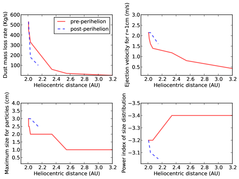
Figure 12: As in Fig. 4, but for comet 78P/Gehrels 2.

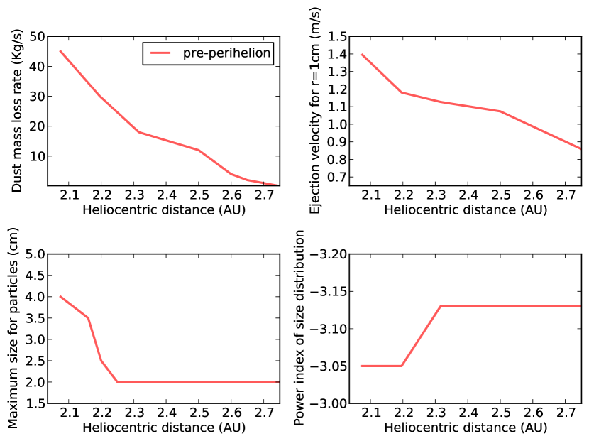
Figure 13: As in Fig. 4, but for comet 115P/Maury.

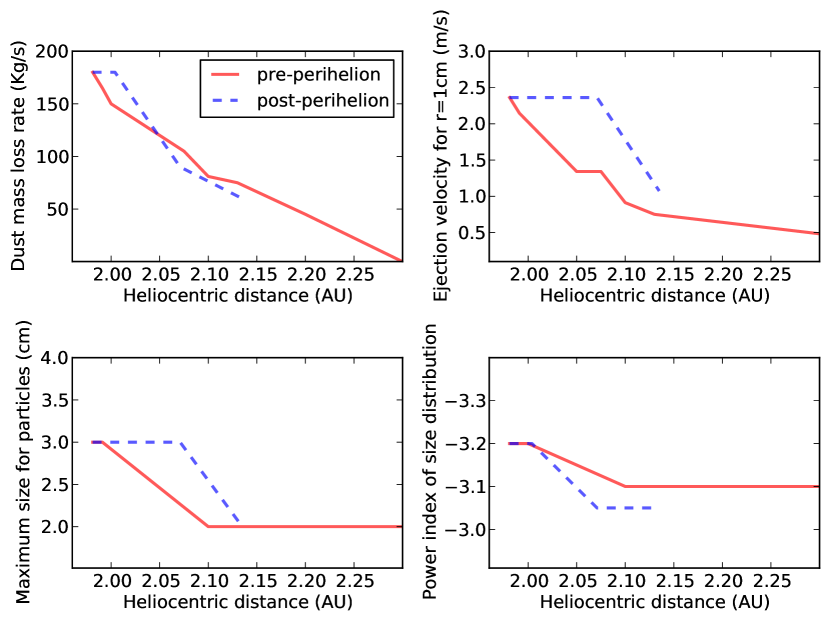
Figure 14: As in Fig. 4, but for comet 118P/Shoemaker-Levy 4.

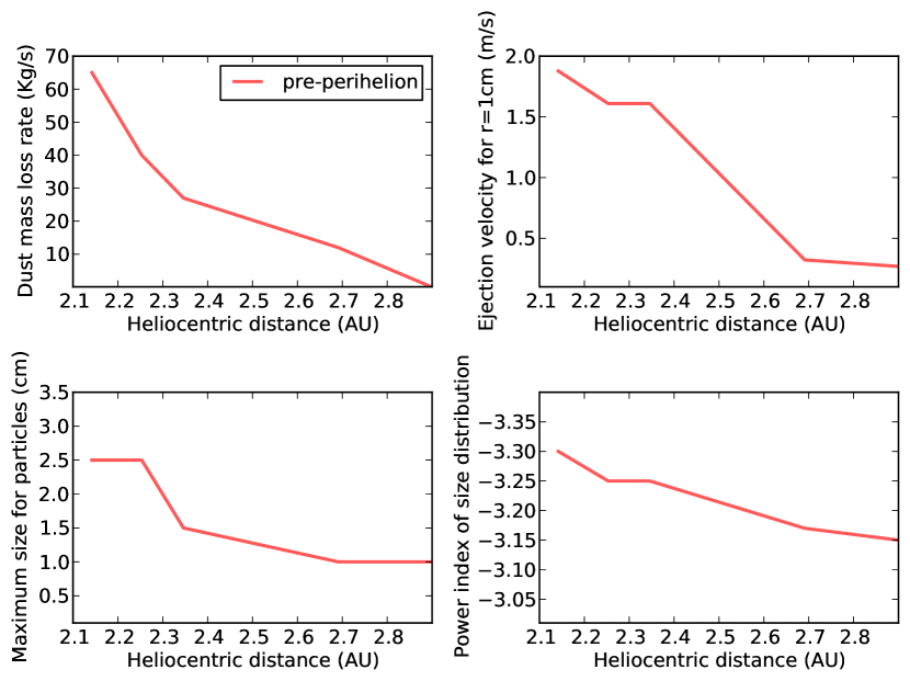
Figure 15: As in Fig. 4, but for comet 123P/West-Hartley.

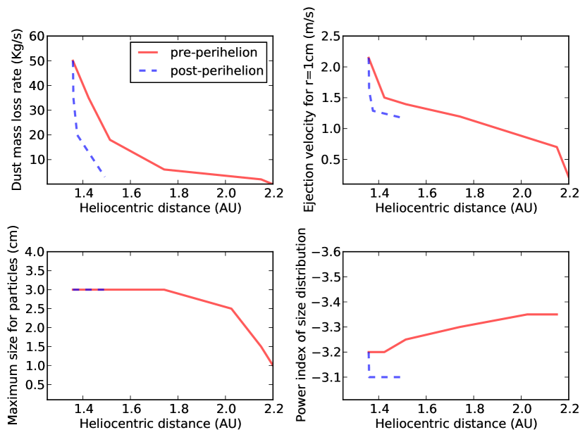
Figure 16: As in Fig. 4, but for comet 157P/Tritton.

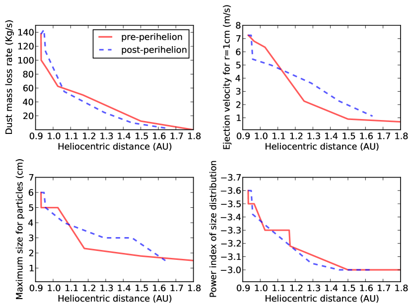
Figure 17: As in Fig. 4, but for comet 185P/Petriew.

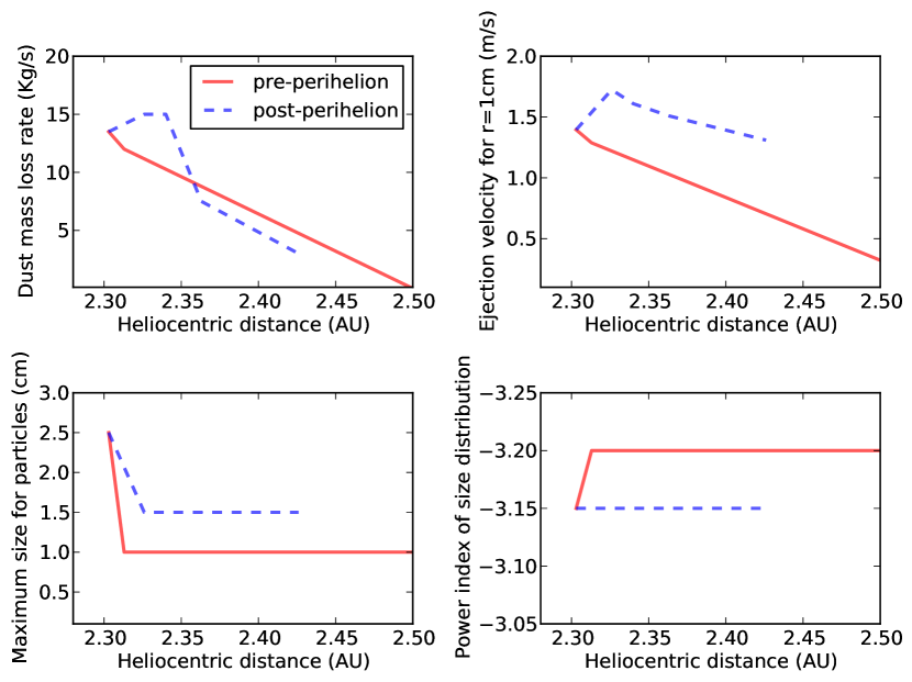
Figure 18: As in Fig. 4, but for comet P/2011 W2 (Rinner).

Appendix C Comparison between observational data and models

In this appendix (figures 19 to 25), we show the comparison of the observational data and the models proposed in section 4, which describe the dust environments of the comets of the sample, as in Fig. 5.

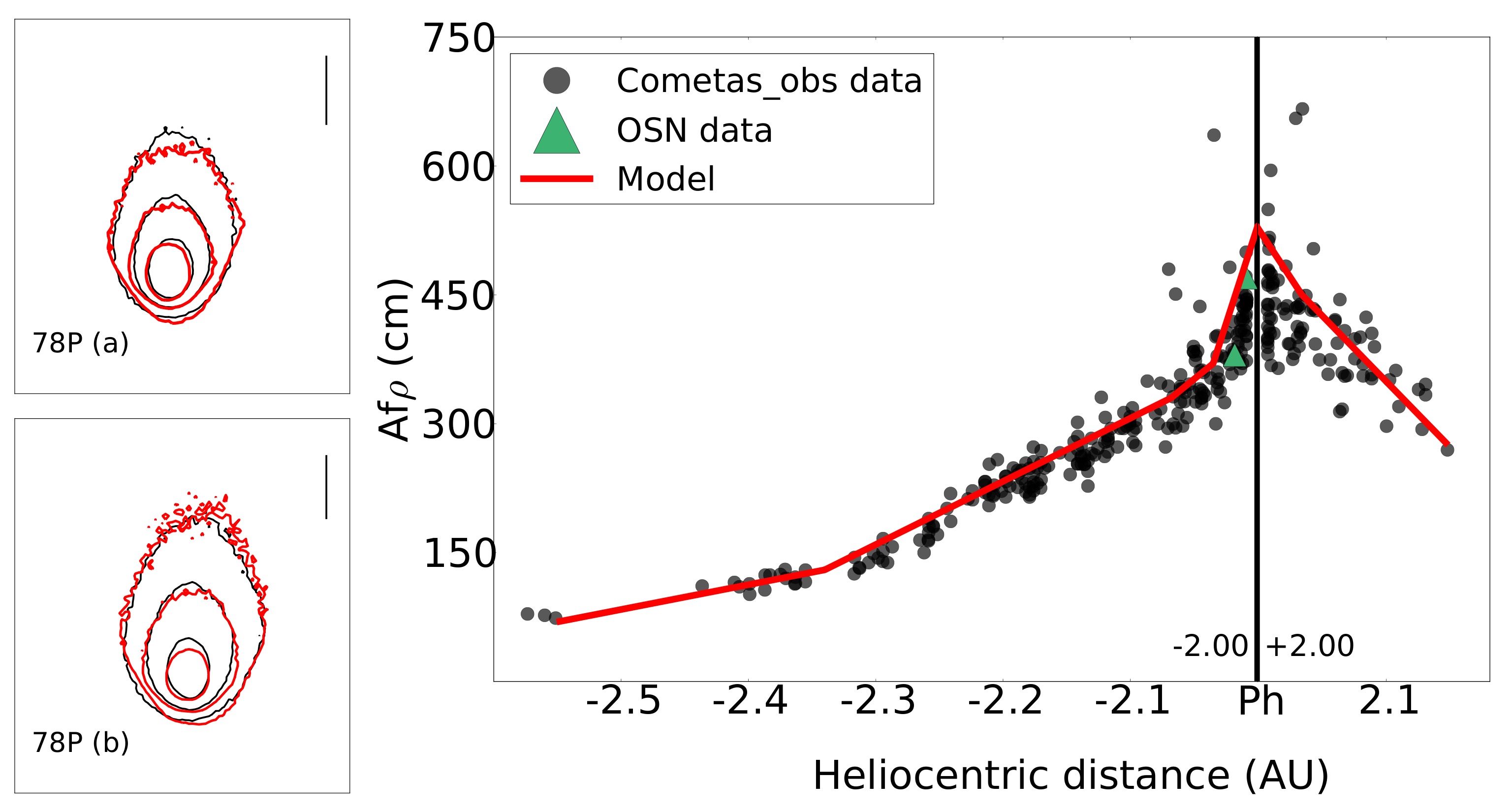
Figure 19: As in Fig. 5, but for comet 78P/Gehrels 2. Isophote fields: (a) December 19, 2011. (b) January 4, 2012. In both cases the isophote levels are $0.55\times 10^{-12}$, $2.65\times 10^{-13}$, and $1.35\times 10^{-13}$ SDU.

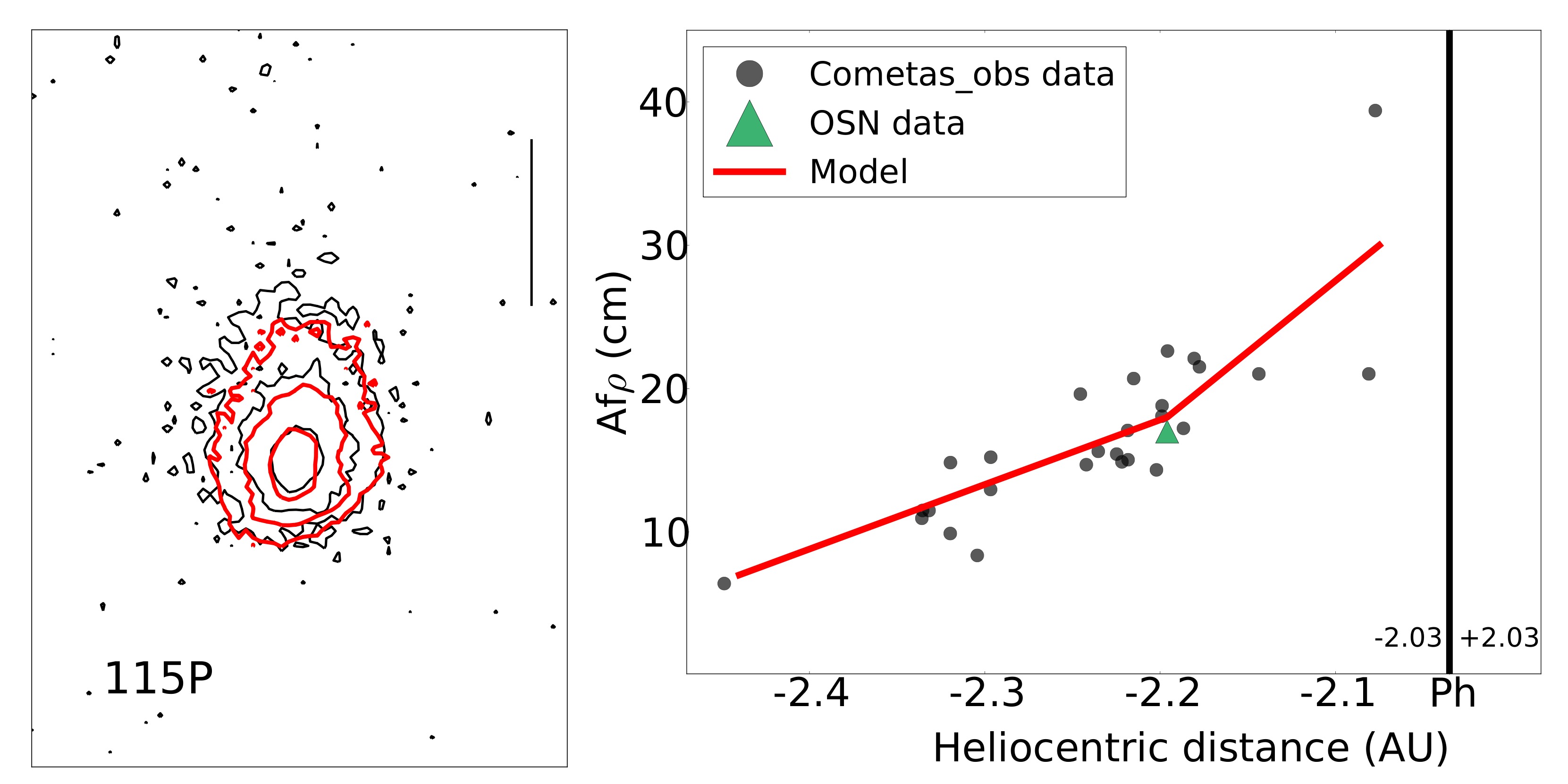
Figure 20: As in Fig. 5, but for comet 115P/Maury. Isophote fields: July 15, 2011. Isophote levels are $1.00\times 10^{-13}$, $3.00\times 10^{-14}$, and $1.30\times 10^{-14}$ SDU.

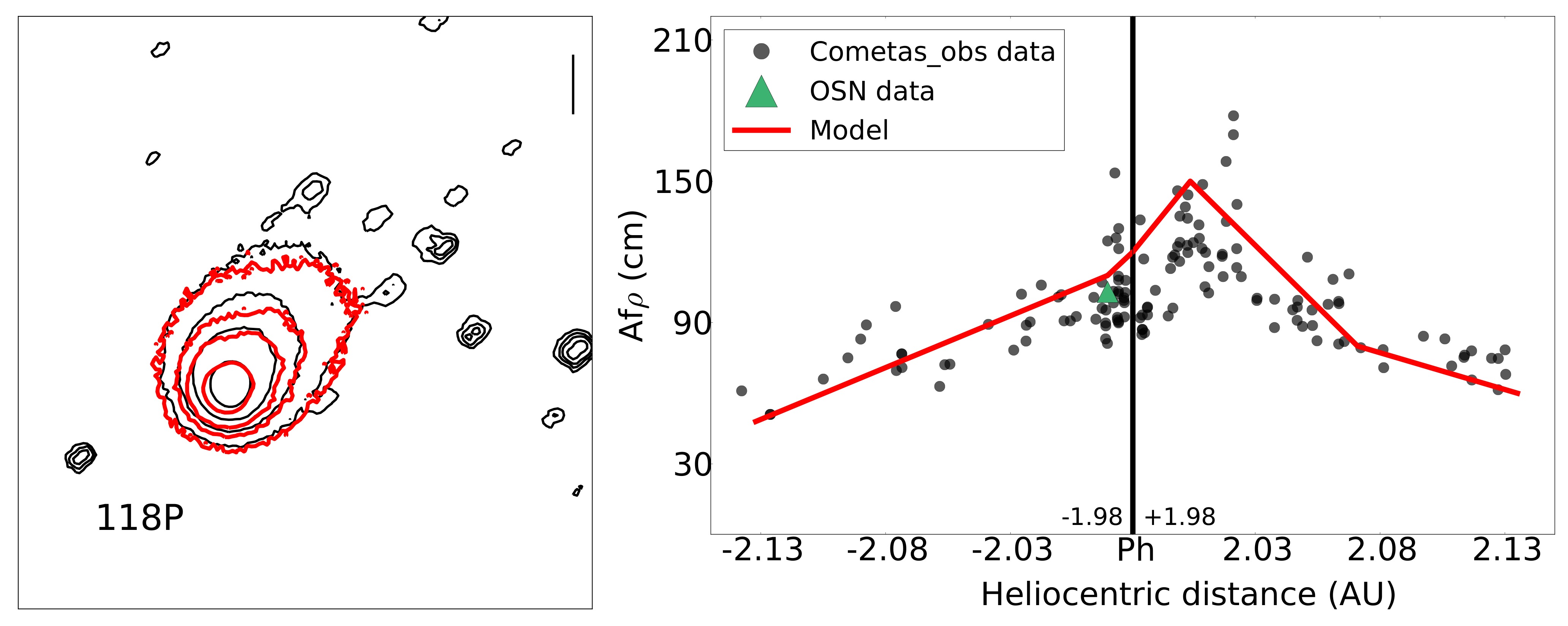
Figure 21: As in Fig. 5, but for comet 118P/Shoemaker-Levy 4. Isophote fields: December 12, 2009. Isophote levels are $1.50\times 10^{-13}$, $6.00\times 10^{-14}$ $3.50\times 10^{-14}$, and $2.00\times 10^{-14}$ SDU.

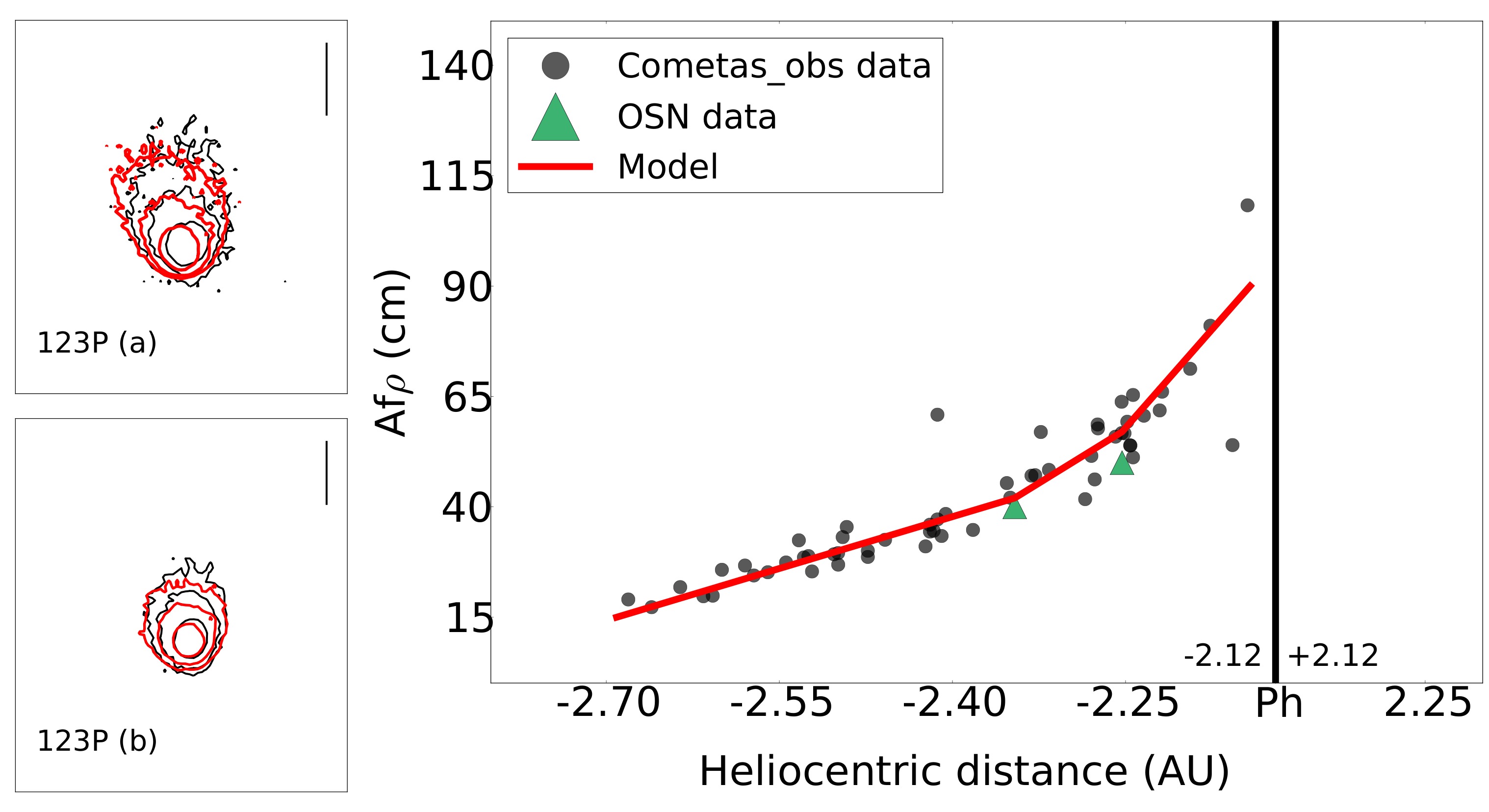
Figure 22: As in Fig. 5, but for comet 123P/West-Hartley. Isophote fields: (a) February 26, 2011. (b) March 31, 2011. Isophote levels are 1.00$\times{10^{-13}}$, 0.35$\times{10^{-13}}$, and 0.15$\times{10^{-13}}$ SDU in (a) and 1.50$\times{10^{-13}}$, 0.50$\times{10^{-13}}$, and 0.25$\times{10^{-13}}$ SDU in (b).

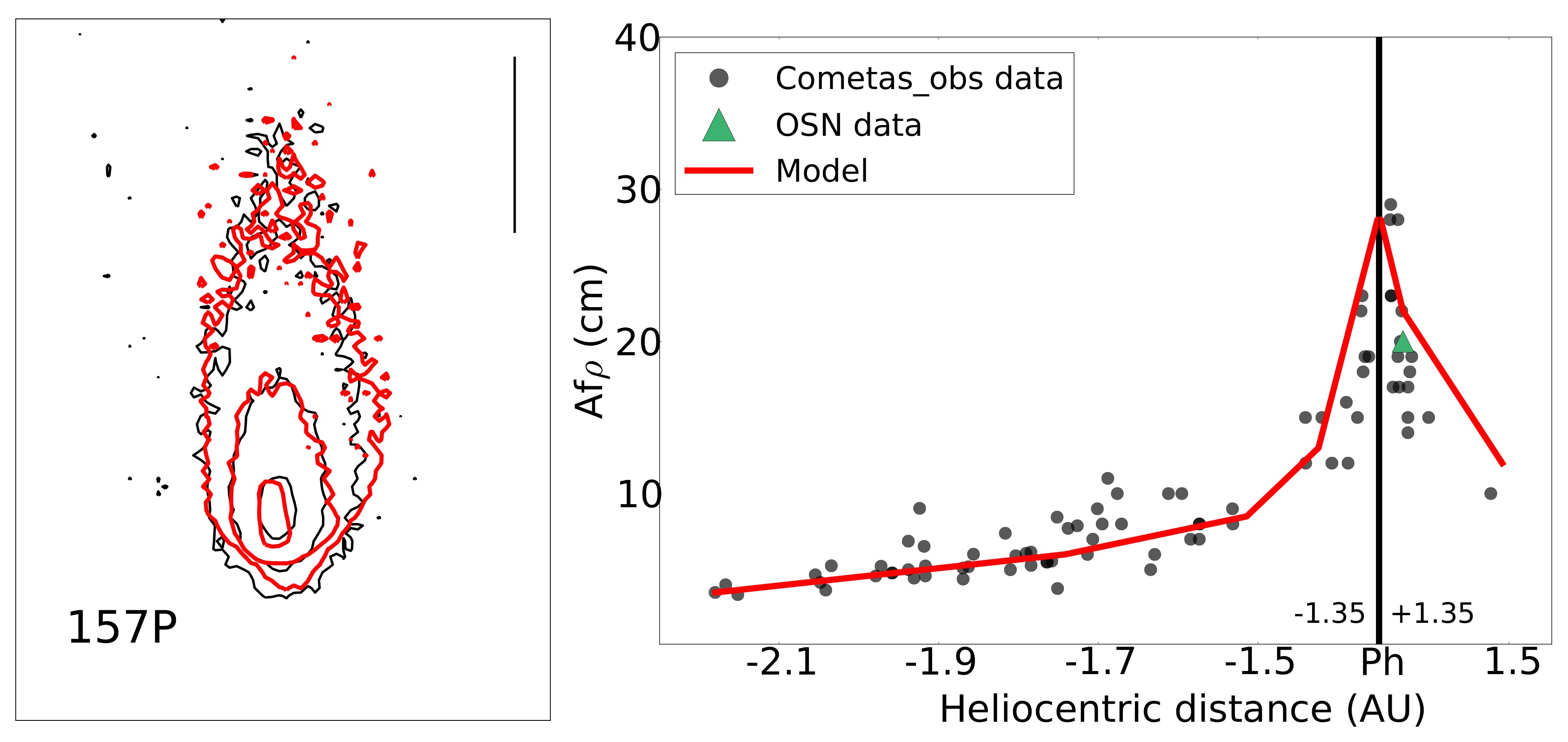
Figure 23: As in Fig. 5, but for comet 157P/Tritton. Isophote fields: March 10, 2010. Isophote levels are $6.00\times 10^{-13}$, $0.75\times 10^{-13}$, and $2.65\times 10^{-14}$ SDU.

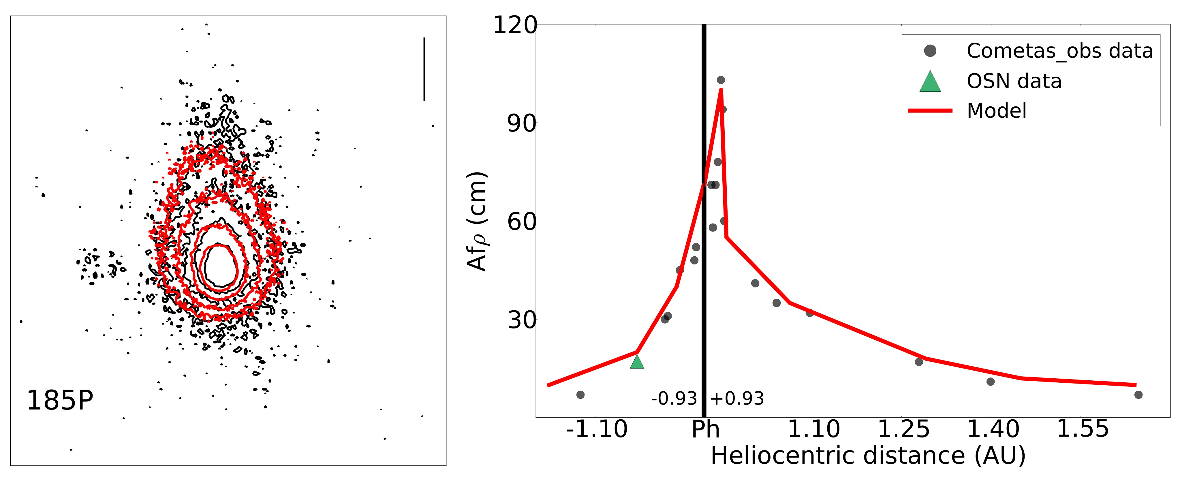
Figure 24: As in Fig. 5, but for comet 185P/Petriew. Isophote fields: July 15, 2012. Isophote levels are $1.80\times 10^{-13}$, $1.00\times 10^{-13}$ $0.60\times 10^{-13}$, and $0.35\times 10^{-13}$ SDU.

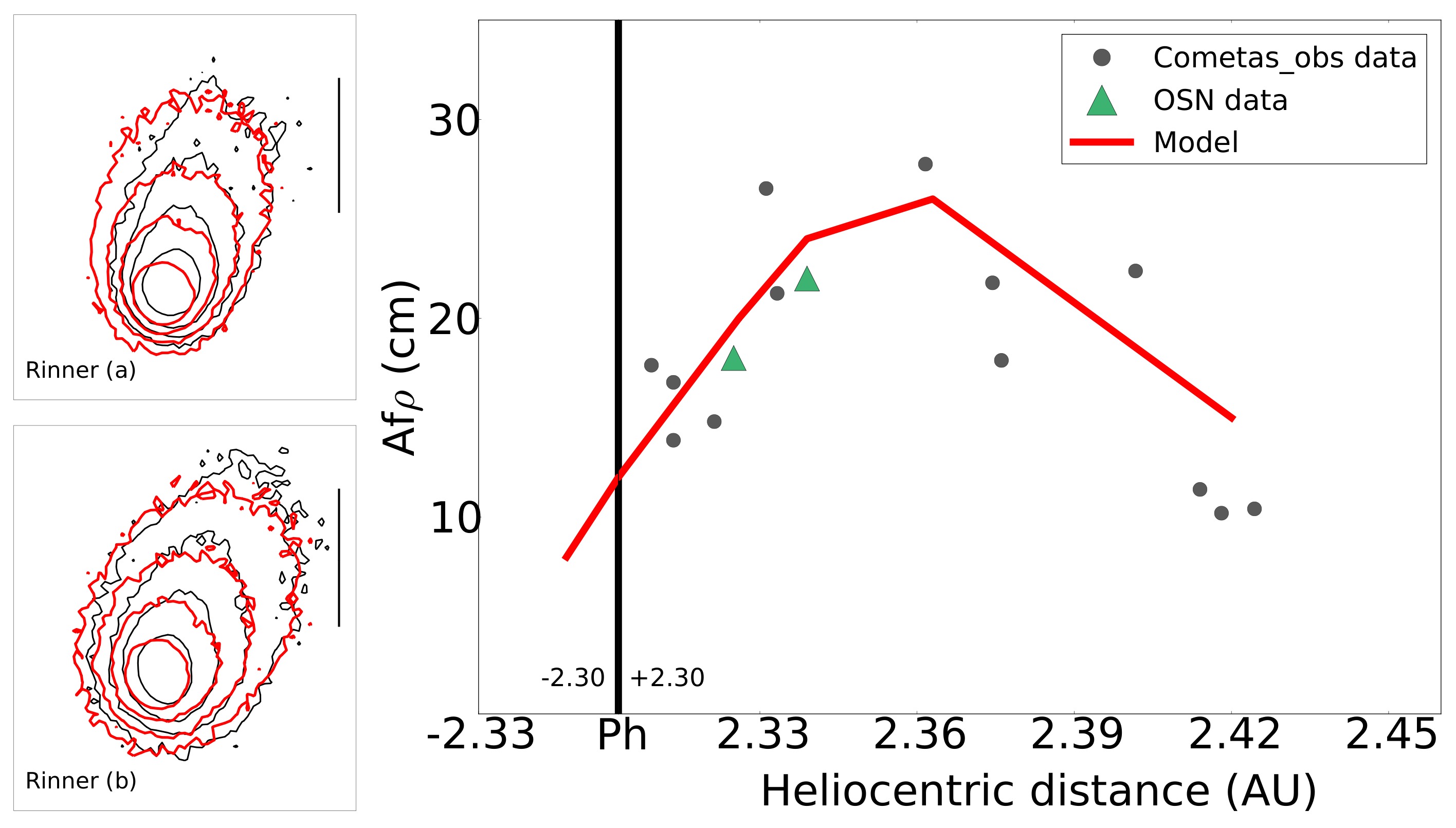
Figure 25: As in Fig. 5, but for comet P/2011 W2 (Rinner). Isophote fields: (a) December 22, 2011. (b) January 4. In both cases the isophote are 6.00$\times{10^{-14}}$, 2.70$\times{10^{-14}}$, 1.50$\times{10^{-14}}$, and 0.80$\times{10^{-14}}$ SDU.