High-energy emissions from the gamma-ray binary LS 5039

Abstract

We study mechanisms of multi-wavelength emissions (X-ray, GeV and TeV gamma-rays) from the gamma-ray binary LS 5039. This paper is composed of two parts. In the first part, we report on results of observational analysis using four year data of Fermi Large Area Telescope. Due to the improvement of instrumental response function and increase of the statistics, the observational uncertainties of the spectrum in $\sim$100-300 MeV bands and $>10$GeV bands are significantly improved. The present data analysis suggests that the 0.1-100GeV emissions from LS 5039 contain three different components; (i) the first component contributes to $<$1GeV emissions around superior conjunction, (ii) the second component dominates in 1-10GeV energy bands and (iii) the third component is compatible to lower energy tail of the TeV emissions. In the second part, we develop an emission model to explain the properties of the phase-resolved emissions in multi-wavelength observations. Assuming that LS 5039 includes a pulsar, we argue that both emissions from magnetospheric outer gap and inverse-Compton scattering process of cold-relativistic pulsar wind contribute to the observed GeV emissions. We assume that the pulsar is wrapped by two kinds of termination shock; Shock-I due to the interaction between the pulsar wind and the stellar wind and Shock-II due to the effect of the orbital motion. We propose that the X-rays are produced by the synchrotron radiation at Shock-I region and the TeV gamma-rays are produced by the inverse-Compton scattering process at Shock-II region.

1 Introduction

The gamma-ray binary is a class binary system emitting high-energy (GeV and/or TeV) gamma-rays, and comprises a compact object (neutron star or black hole) and a high-mass OB star (see Dubus 2013 for recent review on the gamma-ray binaries). Their radiation spectra have a peak in $\nu F_{\nu}$ around GeV energy bands, and extends up to $1-10$TeV energy bands. Five gamma-ray binaries have been detected so far, namely, PSR B1259-63/LS2883 system (Aharonian et al. 2005), LS 5039 (Aharonian et al. 2006), LS I$\mathrm{+61^{o}}$ 303 (Albert et al. 2006), 1FGL J1018.6-5856 (Ackermann et al. 2012) and H.E.S.S. J0632+057 (Hinton et al. 2009). PSR B1259-63/LS 2883 is the only binary system for which the compact object has been confirmed to be a young pulsar.

The GeV gamma-ray observation of the $Fermi$ telescope provides a new challenge for understanding of the non-thermal emission process around gamma-ray binary. The Fermi has revealed that different systems show different properties of the GeV emissions. PSR B1259-63/LS 2883 showed a weak and flare-like emissions during the 2010-2011 periastron passage (Abdo et al. 2011; Tam et al. 2011). The GeV emissions from LS 5039, LS I$\mathrm{+61^{o}}$ 303 and 1FGL J1018.6-5856 are observed for entire orbit, and the spectra are fitted by a power-law plus exponential cut-off form with a cut-off energy around several GeV. The emissions from LS I$\mathrm{+61^{o}}$ 303 show a long-term variability related with the 1667 day super-orbital period in radio (Ackermann et al. 2013). No detection of the GeV emissions has been reported for H.E.S.S. J0632+057.

The gamma-ray binary LS 5039 has been known as a ralatively compact binary system, for which the separation between two component is $\sim 0.1-0.2$ AU and the compact object is moving around an O6.5V main sequence star with a short orbital period $P_{ob}\sim 3.9$ days and a moderate eccentricity ($e\sim 0.24-0.35$, Casares et al. 2005; Aragona et al. 2009; Sarty et al. 2011). The binary system is a source of non-thermal emission in radio (Mold${\rm\acute{o}}$n et al. 2012), X-ray (Takahashi et al. 2009), and gamma-ray (Abdo et al. 2009 for GeV; Aharonian et al. 2006 for TeV) bands, and exhibits temporal variations in its emission and spectrum.

The modulating GeV emission from LS 5039 has been confirmed by the $Fermi$-LAT (Abdo et al. 2009). The pattern of the orbital modulation of GeV emissions shows in anti-phase with X-ray and TeV gamma-ray emissions (c.f. Figure 12); the observed GeV flux (or X/TeV fluxes) becomes maximum around the superior conjunction (or inferior conjunction) and becomes minimum around the inferior conjunction (or superior conjunction). The spectrum in 0.1-10GeV bands is harder when the emission is weaker. The phase-averaged spectrum shows a cut-off around $\sim 2$GeV, and but Hadasch et al. (2012) found an emission feature above 10 GeV, which will be compatible to lower energy tail of the TeV emissions.

The origin of the GeV emissions from the LS 5039 has been remained to be solved. Because the spectral shape of LS5039 measured by Fermi resembles to those of the gamma-ray emitting pulsars, it has been suggested that LS 5039 includes a young pulsar and the emissions from the magnetosphere or the cold-relativistic pulsar wind produces the GeV emissions (Sierpowska-Bartosik & Torres 2007; Kapala et al. 2010; Torres 2011). On the other hand, the inverse-Compton scattering process of the pulsar wind accelerated by the inter-binary shock was also proposed to explain the GeV emissions (Yamaguchi & Takahara 2012; Zabalza et al. 2013).

The main purposes of this study are (1) to present results of the observational analysis using 4-year Fermi data, which provide us a more detailed information on the GeV emissions from LS 5039, and (2) to develop a model to discuss the emission processes of the X-ray, GeV and TeV gamma-rays. The present paper is composed of two parts. In the first part, we report on results of four year observations of the Fermi. Although Hadash et al. (2012) found the emissions above 10 GeV with 2.5yr $Fermi$ data, the large uncertainty in the phase-resolved spectra in those energies prevents us to understand the detailed spectral behavior above 10 GeV. Furthermore, the emissions around 100MeV are strongly affected by the background model. In this paper, therefore, we perform a more detailed analysis with updated instrument response function to obtain more solid understanding of the spectral behavior in 100MeV and $>10$GeV energy bands.

In the second part, we will develop the emission model, in which the emissions from magnetospheric outer gap and from cold-relativistic pulsar wind contribute to the GeV emissions of LS 5039, and will compare the predicted emission properties with the results of Fermi observation. We will also study the X-ray and TeV gamma-ray emissions from the intra-binary shock and will discuss the properties of the phase-resolved spectra in the multi-wavelength bands (X-ray, GeV and TeV). In section 2, we will report on the results of our analysis of the four year Fermi data. We will describe the emission model in section 3 and compare the model predictions with the results of the multi-wavelength observations in section 4. Discussion and a brief summary are given in sections 5 and 6, respectively.

2 Data analysis and results of the Fermi data

2.1 Data set

In this study, we used data collected starting 2008 August 14 and extending until 2012 May 19. The observation time was limited by the availability of the timing model of the nearby gamma-ray pulsar, PSR J1826-1256, which was needed for removing the contribution of the pulsar. The timing model was adopted from the Fermi LAT Multiwavelength Coordinating Group (Ray et al., 2011). The data were reduced and analyzed using the Fermi Science Tools package (v9r32p5), available from the Fermi Science Support Center . We selected only events in the Reprocessed Pass 7 ’Source’ class and used the P7REP_SOURCE_V15 version of the instrumental response functions. To reduce contamination from the Earth’s albedo, we excluded time intervals when the region of interest (ROI) was observed at zenith angles greater than 100° or when the rocking angle of the LAT was greater than 52°. To minimize background from the nearby gamma-ray pulsar, PSR J1826-1256, we excluded events arriving in the pulse phase intervals 0.05-0.2 and 0.6-0.75 of the pulsar.

2.2 Spectral analysis

The gtlike tool was used for spectral analysis. We used photons between 0.1 and 300 GeV within a $20\arcdeg\times 20\arcdeg$ ROI centered at the position of LS 5039. For source modeling, all 2FGL catalog sources (Nolan et al., 2012) within $19\arcdeg$ of the ROI center, the galactic diffuse emission (gll_iem_v05.fit) and isotropic diffuse emission (iso_source_v05.txt) were included.

2.2.1 Phase-averaged spectrum

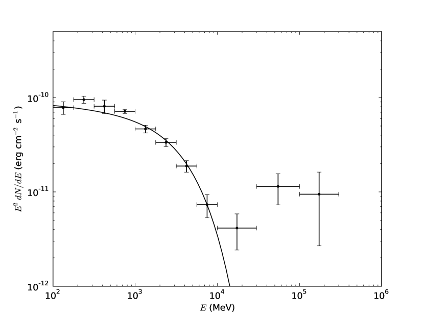
Figure 1: Phase-averaged spectrum of LS 5039. The solid line shows the best-fit model for the full energy band.

We modeled LS 5039 with a power law with an exponential cutoff

$$\frac{dN}{dE}=N_{0}\left(\frac{E}{E_{0}}\right)^{-\Gamma}\exp\left(-\frac{E}{E_{cutoff}}\right).$$ (1)

The spectral types of other point sources in 2FGL are modeled according to the spectral types in the catalog, with the spectral parameters of sources more than $10\arcdeg$ away from the ROI center fixed to the catalog values. The best-fit parameters are $\Gamma=2.06\pm 0.02_{stat}$ and $E_{cutoff}=3.42\pm 0.17_{stat}$ GeV.

Spectral points were obtained by performing a fit in each energy band, fixing the spectral parameters of sources more than 4° away from the ROI center, leaving the flux normalization constants of all other sources and the diffuse background free. The sources that were left free were modeled by power laws. In addition, an initial fit was performed and sources with TS $<0$ in that energy band were removed. Figure. 1 shows the phase-averaged spectrum. Significant emission is observed at E $>$ 10 GeV, in agreement with Hadasch et al. (2012) and Ackermann et al. (2013).

2.2.2 Phase-resolved spectra

Figure 2: Phase-resolved spectra of LS 5039 in SUPC phase (left) and INFC phase (right). The results obtained by Hadasch et al. (2012) are also displayed for comparison. The solid lines show the bet-fitting functions described in section 2.2.2.

We first performed phase-resolved analysis following the H.E.S.S. analysis by Aharonian et al. (2006). We set phase zero at the periastron( $\phi=0$ with MJD=51942.59) and divided one orbit into two phases, that is, the superior conjunction phase (SUPC phase, $0<\phi<0.45$ and $0.9<\phi<1$), which includes SUPC ($\phi=0.06$), and inferior conjunction phase (INFC phase, $0.45<\phi<0.9$), which includes INFC ($\phi=0.72$). We performed similar likelihood analysis in the two phase intervals. In the fitting, all the spectral parameters of LS 5039 were left free, while other spectral parameters were fixed to the phase-averaged values, except for the flux normalization parameters of sources within 5°of the ROI center and the galactic and isotropic diffuse emissions. The best-fit parameters for the SUPC (INFC) are $\Gamma=1.96\pm 0.09_{stat}$ ($1.89\pm 0.12_{stat}$) and $E_{cutoff}=2.86\pm 0.57_{stat}$ ($3.58\pm 0.97_{stat}$) GeV. The spectrum is shown in Figure 2. It is found that the flux in $\sim$100-300 MeV has noticeably decreased compared with previous studies done by Abdo et al. (2009) and Hadasch et al. (2012). This can be due to the improvement in instrumental response functions and data from Pass 6 to Reprocessed Pass 7. The flux beyond $\sim 10$GeV is also increased compared with the previous studies, which is also seen in other results with the Reprocessed Pass 7 data (e.g. see Bregeon et al. 2013).

Due to the increased statistics in this study, we are allowed to divide the observation time into more orbital phase bins. We divided the observation time into three equally spaced orbital phase bins: $[0.17,0.5]$ (bin 1), $[0.5,0.83]$ (bin 2, INFC) and $[0.83,1]\cup[0,0.17]$ (bin 3, SUPC). Both the first and second intervals touch the apastron, but only the second interval contains the INFC. This cut is chosen to better isolate the INFC from the apastron. In addition, the first and second phase bins exclude the SUPC and the third phase bin includes the emissions at the SUPC. The results are shown in Figure. 3 for comparing with results of the theoretical model discussed in section 3. We can see in the figure that the spectra of two orbital bins excluding the superior conjunction (upper panels) have a clear spectral cut-off at $\sim 2$ GeV and the spectra below 10GeV resemble each other. At the phase bin containing the SUPC (lower left panel), an enhancement at $0.1-0.3$ GeV is exclusively seen, and the spectrum below 10GeV is softer than other two phase bins. This suggests that the emissions below 10 GeV are composed of the two components, that is, one contributes to emissions around the SUPC in $<1$GeV bands and other dominates in the 1-10GeV emissions for entire orbit. As we can see in Figure 3, the change of the spectral slope at around 20 GeV in each phase bin suggests existence of an additional component that is compatible to lower energy tail of the TeV emissions

Figure 3: Phase-resolved spectra and the photon index of GeV gamma-ray emissions from LS 5039. Top-left, top-right and bottom-left show the spectra for the orbital interval $0.17<\phi<0.5$, $0.5<\phi<0.83$ and $0.83<\phi<0.17$, respectively. Bottom-right shows the photon index fitted by a single power-law function on 0.2-300GeV. The results of current Fermi data analysis are represented by the filled circles. The solid lines show the results of the theoretical model (section 3), which includes emissions from the outer gap (dashed lines), the cold-relativistic pulsar wind (dotted lines) and the shocked pulsar wind (dashed-dotted lines).

Figure 4: Variation of the integrated flux in $>0.2$GeV bands (left panel) and $>1$GeV bands (right panel). The symbols and the lines correspond to the same case as Figure 3.

2.3 Orbital light curves

To obtain light curves, we performed likelihood analysis similar to Section 2.2.2. The orbital modulation for the flux is summarized in Figure 4, in which the left and right panels display the light curves in two energy bands, 0.2-300 GeV and 1-100 GeV, respectively. In Figure 4, results of the theoretical model are also displayed for comparisons. The observed trends of flux modulation of the two energy bands are similar, but the amplitudes in the modulations are significantly different. The flux including lower energy photons (0.2-300 GeV) is modulated by a factor of $\sim 5$ while that in the high energy band (1-100GeV) is modulated by only a factor of $\sim 2$. This indicates that the variation of spectral hardness along the orbital phase is mainly due to the modulation in the low energy band rather than the high energy band, and the high energy bands are dominated by a component which does not vary with the orbital phase. This could also support the hypothesis that the GeV emissions from LS 5039 are composed of several components with different characteristic energies. This feature is more clearly seen in our results than the results in previous studies. To qualitatively describe the evolution of the hardness of the emissions, we extracted the photon index of each phase interval by assuming a simple power law in 0.2-300 energy bands,

$$\frac{dN}{dE}=N_{0}\left(\frac{E}{E_{0}}\right)^{-\Gamma}.$$ (2)

It is clear from Figure 1 that there is a curvature in the spectra, and a single power law function would not be appropriate at some orbital-phases. However, because of the reduced statistics in individual phase bins, it is not possible to distinguish a simple power law from a power law with exponential cutoff with statistical significance in some bins. A fit with a simple power law can provide a quantitative indicator of the hardness of the spectrum. The result is shown in Figure. 3 (lower right panel). The spectrum is the softest around SUPC and hardest in a broad region centered around the apastron ($\phi=0.5$).

In summary, the results of the four year observations by $Fermi$ improve our understanding of the GeV emissions from LS 5039. The current results suggest that 0.1-100GeV emissions from LS 5039 are likely composed of the three different components (i) the first component contributes to $<$1GeV emissions around superior conjunction, (ii) the second component dominates in 1-10GeV energy bands for entire orbit and (iii) the third component is compatible to lower energy tail of the TeV emissions.

3 Theoretical model

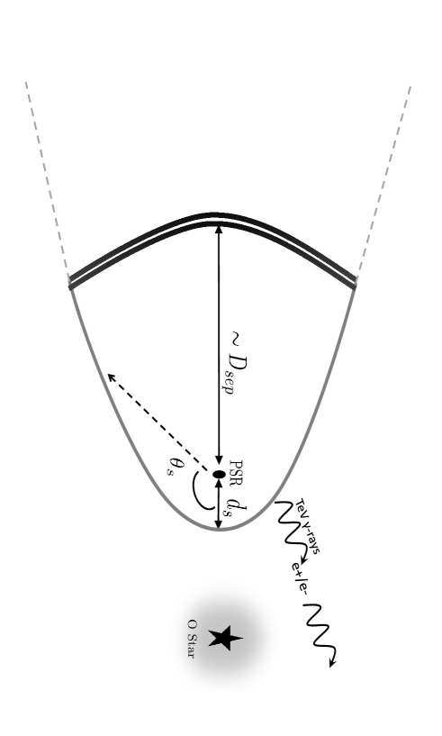
Figure 5: Schematic view of proposed picture of LS 5039 system. LS 5039 comprises a pulsar and an O star, and the interaction between the pulsar wind and the stellar wind from the companion star forms a termination shock (Shock-I, thick-solid line). The distance to shock apex ($d_{s}$) from the pulsar is determined by the balance between the pulsar wind pressure and stellar wind pressure. The effect of the orbital motion of the pulsar also produces a termination shock in opposite direction of the companion star (Shock-II, double-solid lines). The distance to shock from the pulsar is of order of the orbital separation ($D_{sep}$), for which the ram pressure of the stellar wind owing to Coriolis force and the ram pressure of the pulsar in balance. The GeV emissions are mainly produced by the curvature radiation in the magnetospheric outer gap and by the inverse-Compton scattering of the cold-relativistic pulsar wind. The synchrotron process and inverse-Compton process of the shocked pulsar wind produce the X-rays and TeV gamma-rays, respectively. The TeV gamma-rays emitted from the shocked pulsar wind create new electrons and positron pairs, and they initiate the pair-creation cascade, if they propagate toward the companion star.

In the last section, we discussed the evidence of two components of the emissions in 0.1-10GeV bands observed by the $Fermi$. In this paper, we will propose that the emissions in 1-10GeV energy band are dominated by the magnetospheric emissions, while $\sim 0.1$GeV gamma-rays around the superior conjunction are mainly produced by the emissions from the cold-relativistic pulsar wind. Hence our model predicts that the emissions in 1-10 GeV energy band are pulsed.

Figure 5 shows the schematic view of the LS 5039 system discussed in this paper. Our model assumes that LS 5039 includes a pulsar. The pulsar is wrapped by the termination shocks (section 3.1), where the pulsar wind is stopped. The emissions from the magnetosphere (section 3.2) and the inverse-Compton scattering process of the cold-relativistic pulsar wind (section 3.3) contribute to the observed GeV emissions. The synchrotron radiation and the inverse-Compton process of the shocked pulsar wind produce the X-rays and TeV gamma-rays, respectively (section 3.4).

We note that the shock geometry applied in this study (c.f. section 3.1) resembles to one presented in Zabalza et al. (2013), who applied two shock regions; the first shock (Shock-I) is located between the pulsar and the companion star, and the second shock (Shock-II) is opposite direction from the companion star. Both our model and Zabalza et al. (2013) assume that TeV gamma-rays are mainly produced by the Shock-II region (c.f. section 4.2). Main difference between us and Zabalza et al. (2013) is X-ray/GeV emission processes. Our model will predict that the particles accelerated at the Shock-I produce the X-rays via synchrotron radiation, while Zabalza et al. (2013) proposed that the particles accelerated at Shock-I produce the Gev emissions via the IC process. For emissions in 0.1-10GeV bands, we expect that the emissions are mainly produced by the magnetospheric particles in the outer gap and the cold-relativistic pulsar wind. Since Zabalza et al. (2013) mainly focused on the GeV/TeV gamma-ray emission process and had a difficulty to explain the X-ray emission process, we will develop an emission model covering from X-ray to TeV energy bands.

3.1 Shock geometry

We assume that two kinds of termination shock exist around the pulsar (c.f. Figure 5). First, balancing between the pressures of the pulsar wind and the stellar wind produces cone-shape shock between the pulsar and the companion star (Shock-I). The opening angle and the geometry of the cone-shape shock are determined by ratio of the momenta of the two winds (e.g. Eichler & Usov 1993; Canto et al. 1996),

$$\eta\equiv\frac{L_{sd}}{\dot{M}v_{w}c},$$ (3)

where $L_{sd}$ is the spin down energy, $\dot{M}$ is the mass loss rate of the outflow from the companion star and $v_{w}$ is the velocity of the outflow. The distance to the shock apex from the pulsar can be determined by $r_{apex}=D_{sep}\eta^{1/2}/(1+\eta^{1/2})$, where $D_{sep}$ is the separation between two stars. In this paper, we will apply $\eta=0.05$ with $L_{sd}\sim 2\times 10^{36}{\rm erg~{}s^{-1}}$, $\dot{M}\sim 10^{-7}M_{\odot}{\rm yr^{-1}}$ and $v_{w}\sim 2\times 10^{8}{\rm cm~{}s^{-1}}$.

Second, recent results of 2-D hydrodynamic simulation of LS 5039 (e.g. Bosch-Ramon et al. 2012) have suggested that the effect of the orbital motion also produces a pulsar wind termination shock even in opposite direction from the companion star (Shock-II, c.f. double-solid line in Figure 5). The distance from the pulsar is found to be of order of the orbital separation, for which the ram pressure of the stellar wind owing to Coriolis force and the ram pressure of the pulsar are in balance. Zabalza et al. (2013) provided an approximate expression for location of the shock as

$$x_{cor}\sim\sqrt{\frac{L_{sd}v_{w}}{\dot{M}c(2\Omega_{o})^{2}}},$$ (4)

where $\Omega_{o}$ is the angular velocity of the pulsar around the star. With $\Omega_{o}\sim 10^{-5}~{}{\rm s^{-1}}$, the expression (4) yields $x_{cor}\sim 0.15{\rm AU}\sim 1-2D_{sep}$. In this paper, we assume $r_{s}=1.5D_{sep}$ as the radial distance to the Shock-II from the pulsar. Figure 6 shows the distance to the shock as a function of angle measured from the direction of the companion star.

It has been pointed out that 3D simulation will give a more complex structure of Shock-II, because the instability will develop faster and more disruptive in 3D simulation than 2D (Bosch-Ramon et al. 2012). Because the detailed structure of the shock-II region given by the 3D simulation has not been known for LS 5039 system, we apply the result of 2-D calculation in this study.

Figure 6: Distance to termination shock from the pulsar with respect to the angle measured ($\theta_{s}$, c.f. Figure 5) from the direction of the companion star. Solid line: Distance to the shock caused by the interaction between the pulsar wind and the stellar wind (Shock-I). The result is for the momentum ration of $\eta=0.05$. Double solid line: Distance to the shock caused by the effect of the orbital motion of the pulsar (Shock-II). In the calculation, we assume $r_{s}=1.5D_{sep}$. The sub-panel in the figure show the separation between two stars as a function of the orbital phase.

3.2 Magnetospheric emission

We calculate the expected spectra of the gamma-ray emissions from the outer gap accelerator in the pulsar magnetosphere (Cheng et al. 1986). In the outer gap, the electrons and positrons are accelerated by the electric field along the magnetic field lines. The accelerated particles emit the GeV gamma-rays through the curvature radiation process. The typical magnitude of the accelerating electric field is

$$E_{||}\sim\frac{f_{gap}^{2}B(R_{lc})R_{lc}}{R_{c}},$$ (5)

where $B$ is the local magnetic field strength, $R_{lc}=c/\Omega$ is the radius of the light cylinder, $R_{c}$ is curvature radius of the magnetic field line, and $f_{gap}$ is the ratio of the gap thickness in the trans-field direction and the light cylinder radius at the light cylinder. The accelerated electrons and positrons produce gamma-rays via the curvature radiation process. The Lorentz factor of the electrons/positrons is estimated by balancing between the acceleration force and back reaction force of the curvature radiation,

$$\Gamma_{e}\sim\left(\frac{3R_{c}^{2}}{2e}E_{||}\right)^{1/4}\sim 2\times 10^{7}\left(\frac{f_{gap}}{0.1}\right)^{1/2}\left(\frac{\Omega}{10^{2}{\rm s^{-1}}}\right)^{1/2}\left(\frac{B(R_{lc})}{10^{5}{\rm G}}\right)^{1/4}\left(\frac{R_{c}}{R_{lc}}\right)^{1/4}.$$ (6)

Typical energy of the curvature radiation is found to be of order of $\sim$GeV,

$$E_{c}\sim\frac{3hc\Gamma_{e}^{3}}{4\pi R_{c}}\sim 800\left(\frac{\Gamma_{e}}{2\cdot 10^{7}}\right)^{3}\left(\frac{\Omega}{10^{2}{\rm s^{-1}}}\right)\left(\frac{R_{c}}{R_{lc}}\right)^{-1}{\rm MeV}.$$ (7)

The luminosity of the gamma-ray emissions from the outer gap becomes

$$L{\gamma}\sim f^{3}_{gap}L_{sd}\sim 3.8\times 10^{35}f_{gap}^{3}\left(\frac{P}{0.1{\rm s}}\right)^{-4}\left(\frac{B_{s}}{10^{12}{\rm G}}\right)^{2}{\rm erg~{}s^{-1}},$$ (8)

where $L_{sd}=2(2\pi)^{4}B^{2}_{s}R^{6}_{s}/(3c^{3}P^{4})$ is the spin down power, $P$ is the pulsar’s spin period, $B_{s}$ is the stellar magnetic field and $R_{s}=10^{6}$cm is the radius of neutron star. The fractional gap thickness is estimated as

$$f_{gap}={\rm min}(f_{m},f_{p}),$$ (9)

where $f_{m}=0.25K(P/0.1{\rm s})^{1/2}$ with $K\sim 2$ and $f_{p}=5.5P^{26/21}(B_{s}/10^{12}{\rm G})^{-4/7}$ (Takata et al. 2010). A more detailed description of the outer gap model can be found in Wang et al. (2010).

3.3 Inverse-Compton emission from cold-relativistic pulsar wind

It is possible that the inverse-Compton (IC) scattering of cold-relativistic pulsar wind off the stellar photons produces high-energy gamma-rays (Ball & Kirk 2000; Khangulyan et al. 2011, 2012). For LS 5039 system, this IC component could play an important role to explain for the observed emissions. As we will show in equation (12), the typical Lorentz factor of the cold-relativistic pulsar wind will be $\Gamma_{0}\sim 10^{4}$. Hence, the inverse-Compton scattering process will be occurred in the Thomson regime. With typical separation of two stars ($D_{sep}\sim 0.1$ AU), the optical depth of IC process will be of order of unity (by ignoring the effect of the collision angle)

$$\tau_{IC}(D_{sep}=0.1{\rm AU})\sim n_{ph}\sigma_{IC}r_{s}\sim 5\left(\frac{\sigma_{IC}}{\sigma_{T}}\right)\left(\frac{T_{eff}}{3\cdot 10^{4}{\rm K}}\right)^{3}\left(\frac{R_{*}}{9R_{\odot}}\right)^{2}\left(\frac{D_{sep}}{0.1{\rm AU}}\right)^{-2}\left(\frac{r_{s}}{0.01{\rm AU}}\right),$$ (10)

where $r_{s}$ is the distance to the shock, $T_{eff}$ is the effective temperature of the companion, and $\sigma_{T}$ is the Thomson cross section. The luminosity becomes of order of

$$L_{IC}\sim\frac{\Gamma_{0}kT_{eff}}{m_{e}c^{2}}L_{sd}\sim 0.03\left(\frac{kT_{eff}}{3{\rm eV}}\right)\left(\frac{\Gamma_{0}}{5\cdot 10^{3}}\right)L_{sd}.$$ (11)

Hence the IC process of the cold-relativistic will produce observable high-energy gamma-rays.

The characteristic energy of the IC photons depends on the Lorentz factor of the cold-relativistic pulsar wind. If the pulsar wind is a kinetically dominated flow, the typical Lorentz factor of the bulk flow will be

$$\Gamma_{W,0}\sim\Gamma_{W,L}\sigma_{L}\sim 10^{4}\left(\frac{\kappa}{10^{5}}\right)^{-1}\left(\frac{L_{sd}}{10^{36}{\rm erg~{}s^{-1}}}\right)^{1/2},$$ (12)

where $\Gamma_{W,L}$ and $\sigma_{L}=B^{2}(R_{lc})/[4\pi\Gamma_{W,L}\kappa m_{e}c^{2}n_{GJ}(R_{lc})]$ are the Lorentz factor and the magnetization parameter of the pulsar wind at the light cylinder, respectively. In addition, $n_{GJ}(R_{lc})=\Omega B(R_{lc})/(2\pi ce)$ is the Goldreich-Julian number density and $\kappa$ is the multiplicity. The observed power of the synchrotron nebulae around the pulsars implies a multiplicity of $\kappa=10^{4-5}$ (De Jager et al. 1996; De Jager 2007; Harding & Muslimov 2011). The radiation per unit energy power unit solid angle of single particle with a Lorentz factor $\Gamma_{W}$ is given by

$$\frac{dP_{IC}}{d\Omega_{1}}={\cal D}^{2}\int_{0}^{\theta_{c}}(1-\beta\cos\theta_{0})I_{b}/h\frac{d\sigma^{\prime}}{d\Omega^{\prime}}d\Omega_{0},$$ (13)

where $d\sigma^{\prime}/d\Omega^{\prime}$ is the differential Klein-Nishina cross section, ${\cal D}=\Gamma_{W}^{-1}(1-\beta\cos\theta_{1})^{-1}$, $\theta_{1}$ and $\theta_{0}$ describe the angle between the direction of the particle motion and the propagating direction of the scattered photons and background photons, respectively. In addition, $I_{b}$ is the stellar photon field and $\theta_{c}=\sin^{-1}R_{*}/r$ expresses the angular size of the star as seen from the point $r$. For the target stellar photon field, we take the stellar radius $R_{*}=9R_{\odot}$, where $R_{\odot}$ is the solar radius, and an effective temperature $kT_{eff}=3.4$eV. With $kT_{eff}=3.4$ eV, the scattering process of the electrons with a Lorentz factor of $\gamma_{e}\geq 2\times 10^{5}$ is occurred in the Klein-Nishina regime (c.f. Figure 9), implying existence of a break in the inverse-Compton spectrum at around $\sim 10^{11}$eV.

A mono-energetic assumption for the distribution of electrons and positions in the pulsar wind had been assumed as a first approach to the problem (e.g. Takata et al. 2009). It is suggested however that the energy distribution as a result of a dissipation of the magnetic energy to the particle energy can be different from the mono-energetic distribution (Sierpowska-Bartosik & Torres 2008 and reference their in). In this paper, we explore the emissions with a relativistic Maxwell distribution of the form,

$$f(r,\Gamma_{W})=K(r)\Gamma^{2}_{W}{\rm exp}\left(-\frac{3\Gamma_{W}}{\Gamma_{0}(r)}\right),$$ (14)

which provides the averaged Lorentz factor of

$$<\Gamma_{W}(r)>\equiv\frac{\int_{1}^{\infty}\Gamma_{W}f(r,\Gamma_{W})d\Gamma_{W}}{\int_{1}^{\infty}f(r,\Gamma_{W})d\Gamma_{W}}\sim\Gamma_{0}(r).$$

We assume that the distance ($r_{i}$) from the pulsar at which the kinetically dominated pulsar wind is formed is smaller than the shock distance, and that the averaged Lorentz factor at $r=r_{i}$ is $\Gamma_{0}(r_{i})=5\times 10^{3}$. The normalization $K(r_{i})$ at $r=r_{i}$ is calculated from

$$m_{e}c^{2}\int_{1}^{\infty}\Gamma_{W}f(r_{i},\Gamma_{W})d\Gamma_{W}=\frac{L_{sd}}{4\pi r_{i}^{2}c}.$$

The Lorentz factor of the pulsar wind evolves with the distance due to the energy loss by IC scattering process. For example, Figure 7 shows the Lorentz factor of the pulsar wind at the shock as a function of the angle measured from the direction of the companion star, where the initial Lorentz factor is $\Gamma_{0}=5\times 10^{3}$. We can see in Figure 7 that for the cold-relativistic pulsar wind propagating toward the companion star ($\theta_{s}\sim 0$),  40-50% of the initial energy is released before the shock, while for the pulsar wind propagating in opposite direction of the companion star ($\theta_{s}\sim\pi$), the energy loss is negligible.

We assume that at each point, “thermalization” is quickly established and the distribution is described by the relativistic Maxwell distribution (14). The radiation power integrated within the distance $r$ is

$$\delta P_{IC}=4\pi\int\int\int r^{2}f(r,\Gamma_{W})\frac{dP_{IC}}{d\Omega_{1}}d\Omega_{1}drd\Gamma_{W}dE_{\gamma},$$

where $E_{\gamma}$ is the energy of scattered photons. The normalization $K(r)$ and the averaged Lorentz factor $\Gamma_{0}(r)$ are calculated with the equations of particle conservation and of the energy conservation, that is,

$$r^{2}\int f(r,\Gamma)d\Gamma=r_{i}^{2}\int f(r_{i},\Gamma)d\Gamma,$$ (15)

and

$$m_{e}c^{2}\int\Gamma_{W}f(r,\Gamma_{W})d\Gamma_{W}+\frac{\delta P_{IC}}{4\pi r^{2}c}=\frac{L_{sd}}{4\pi r_{i}^{2}c},$$ (16)

respectively.

We would like to mention that we additionally calculated the emissions with mono-energetic distribution and single power law distribution of the pulsar wind as well. For the mono-energetic distribution, we found that the shape of the calculated spectra resembles to one calculated with the relativistic Maxwell function. For the power law distribution, we assumed that the particles are accelerated above $\Gamma_{0}(r_{i})\sim 5\times 10^{3}$ with a power law index of $3-4$, which has been predicted by the plasma simulations of the magnetic reconnection process (Zenitani & Hoshino 2005). We found that although the inverse-Compton spectrum extends to very high energy bands, its contribution with the “soft” power law index $3-4$ is much smaller than the shock emissions. Within the present framework of the particle distributions, therefore, the main results discussed in section 4 are not modified.

Figure 7: The ratio of Lorentz factor at the shock and initial Lorentz factor of the cold-relativistic pulsar wind with respect to the angle measured from the direction of the companion star. The cold-relativistic pulsar wind looses the energy via the inverse-Compton scattering off the stellar photons.

Figure 8 summarizes the temporal variations of the integrated flux of IC emissions with respect to the orbital phase. The different curves represent the results for different Earth viewing angles measured from the direction perpendicular to the orbital plane. As we can see in Figure 8, the model light curves tend to have a peak around SUPC. This is (1) because the IC photons emitted toward the Earth are produced by the head-on like collision process, and (2) because SUPC ($\phi\sim 0.06$) is close to the periastron ($\phi=0$), where the separation between two stars becomes minimum and hence the soft photon number density at the location of the pulsar becomes maximum. As a result, the IC process is more efficient around SUPC. Around INFC, the flux becomes minimum, since the IC photons traveling toward the Earth are produced by the tail-on collision process. In Figure 8, we can see that a larger Earth viewing angle predicts a larger amplitude of the modulation. This is because as the Earth viewing angle approaches to the edge on, the amplitude of variation of the collision angle, which is angle between the stellar photons and the pulsar wind that emits photons toward the Earth, along the orbital phase increases. We also find a tendency in Figure 8 that as Earth viewing angle becomes small, the positions of flux maximum and minimum shift toward the periastron ($\phi=0$) and apastron ($\phi=0.5$), respectively. This is related to the fact that IC emissivity depends on (1) the collision angle and (2) the number density of the soft photons. For a larger Earth viewing angle, the effect of the variation of the collision angle with the orbital phase affects more to the variation of the IC flux. In such a case, the flux maximum (or minimum) appears at the superior conjunction (or inferior conjunction). If the Earth viewing angle approaches to zero, the orbital variation of the collision angle is small, and the variation of number density of soft photons at the emission regions mainly causes the variation of the IC flux. In such a case, the IC flux becomes maximum (or minimum) at the periastron (or apastron), where the photon number density at the emission region becomes maximum (or minimum).

Figure 8: Variation of the integrated flux of the inverse-Compton photons from the cold-relativistic pulsar wind. The results are for typical Lorentz factor of $\Gamma_{W,0}=5\times 10^{3}$. The different lines show the results for the different Earth viewing angles measured from the direction perpendicular to the orbital plane. The phase zero $\phi=0$ corresponds to periastron, and the vertical double-dotted lies indicate the positions of the superior conjunction ($\phi=0.06$) and the inferior conjunction ($\phi=0.72$), respectively.

3.4 Shock Emissions

At the shock, the kinetic energy of the pulsar wind is converted into the internal energy of the wind, and the distribution of particles at the shock is assumed to be described by a power law over several decades in energy. The minimum Lorentz factor ($\gamma_{e,min}$) of the shocked pulsar wind particles is assumed to be the average Lorentz factor of the cold-relativistic pulsar wind at the shock ($\Gamma_{0}(d_{s})$, c.f. Figure 7). The maximum Lorentz factor $\gamma_{e,max}$ is determined by balancing between the acceleration time scale $t_{a}\sim\gamma_{e}m_{e}c/(eB)$ and the synchrotron loss time scale $t_{s}\sim 9m_{e}^{3}c^{5}/(4e^{4}B^{2}\gamma_{e})$. In this paper, we will assume $p=2.1$ for the power law index of the distribution of the particles accelerated at the shock.

Since the ratio of the pulsar wind momentum to the stellar wind momentum is much smaller than unity ($\eta\ll 1$), we approximate that the flow of the shocked pulsar wind points radially outwards from the companion star. In this study, we assume that velocity ($v_{PW}$) of the bulk motion of shocked pulsar wind does not change with the radial distance, that is, $v_{PW}(r)=$constant, because the high-energy emission occurs in the vicinity of the shock.

In down stream region, the particles loose their energy via the cooling processes. With the steady state approximation, the evolution of the distribution function $N(r,\gamma_{e})$ is given by

$$\frac{\partial N}{\partial r}+\frac{\partial}{\partial\gamma_{e}}\left(\frac{d\gamma_{e}}{dr}N\right)=Q(\gamma_{e})\delta(r-r_{s}),$$ (17)

where $Q(\gamma_{e})$ is the source function at the shock. The energy loss of the particles is calculated from

$$\frac{d\gamma_{e}}{dr}=\frac{1}{v_{PW}}\left[\left(\frac{d\gamma_{e}}{dt}\right)_{ad}+\left(\frac{d\gamma_{e}}{dt}\right)_{syn}+\left(\frac{d\gamma_{e}}{dt}\right)_{IC}\right].$$ (18)

We apply the adiabatic loss given by

$$\left(\frac{d\gamma_{e}}{dt}\right)_{ad}=\frac{\gamma_{e}}{3n}\frac{dn}{dt}=-\frac{2v_{PW}}{3r},$$ (19)

where $n$ is the particle number density and we apply $nr^{2}=$constant. The synchrotron loss is given as

$$\left(\frac{d\gamma_{e}}{dt}\right)_{syn}=-\frac{4e^{4}B^{2}\gamma_{e}^{2}}{9m_{e}^{3}c^{5}},$$ (20)

where we used the average pitch angle, because we expected that the magnetic field in the shocked pulsar wind is easily randomized. The IC energy loss rate is

$$\left(\frac{d\gamma_{e}}{dt}\right)_{IC}=-\int\int(E-E_{S})\frac{\sigma_{IC}c}{m_{e}c^{2}E_{s}}\frac{dN_{s}}{dE_{s}}dE_{s}dE,$$ (21)

where $dN_{s}/dE_{s}$ is the stellar photon field distribution and $\sigma_{IC}$ is the cross section for the isotropic photon field. We estimate the magnetic field just behind the shock as

$$B(r_{s})=3\left(\frac{L_{sd}\sigma(r_{s})}{r_{s}^{2}c[1+\sigma(r_{s})]}\right)^{1/2},$$ (22)

where $\sigma(r_{s})$ is the magnetization parameter at the shock. In down stream region, we consider that the magnetic field evolves as $B(r)r=$constant.

We assume that the magnitude of the magnetization parameter at the shock depends on the shock distance from the pulsar, because we expect that an energy conversion from the magnetic field to the particle energy of the cold-relativistic pulsar wind gradually decreases the magnetization parameter with the radial distance from the pulsar. Because there is a theoretical uncertainty for the evolution of $\sigma$ with the radial distance, we describe the magnetization parameter at the shock with a single power-law function,

$$\sigma(r_{s})=\sigma(r_{apex,0})\left(\frac{r_{s}}{r_{apex,0}}\right)^{-\alpha},$$ (23)

where $r_{apex,0}$ is the shock apex distance at the periastron. The evolution of the magnetization parameter for the gamma-ray binary PSR B1259-63/LS 2883 system is also suggested to explain the X-ray/TeV emissions (Takata & Taam 2009; Kong et al. 2011, 2012). We will argue in section 5.1 that the index $\alpha$ affects the predicted flux at TeV energy band.

We expect that the high-energy emission processes occure at the vicinity of the shock surface. Figure 9 shows the time scales of the radiation losses; solid, dashed and dotted lines show the time scales of the adiabatic loss, the synchrotron loss, and the IC loss, respectively. The results are for the radial distance $r=0.1$AU from the pulsar in opposite direction of the companion and the magnetic field $B\sim 0.5$ G. Since the time scale of the adiabatic loss ($\sim 3r/2v_{PW}$) represents the crossing time scale of the shock region, we can see in Figure 9 that the crossing time scale of the particles with a Lorentz factor $\gamma_{e}>10^{3}$ is longer than the time scale of the radiation losses, implying the accelerated particles loose most of their energy at the vicinity of the shock surface through the radiation processes. In the present calculation, therefore, we take into account the emissions occurred between the shock distance $r_{s}$ and the radial distance $3r_{s}$, beyond which the emissions of the cooled particles are negligible.

Figure 9: Time scales of the adiabatic loss (solid line), synchrotron loss (dashed line) and IC loss (dotted line). The results are for the radial distance $r=0.1$ AU from the pulsar in opposite direction of the companion star and the magnetic field $B=0.5$G. The turn over of the IC loss at the Lorentz factor $\sim 10^{5}$ is due to the Klein-Nishina effect.

Finally, we expect that effect of the Doppler boosting due to the finite velocity of the shocked pulsar wind is the main reason to cause the temporal variation of the X-ray emissions with the orbital phase. The Doppler boosting introduces an orbital modulation of the emissions that are isotropic in co-moving frame with the flow. Dubus et al. (2010) suggested that the observed orbital modulation of the X-ray emissions from LS 5039 is the result of the Doppler boosting of the shocked pulsar wind with a mildly relativistic speed, $\beta_{PW}\equiv v_{PW}/c\sim 0.15-0.3$. Note that this scenario will be different from the case of the gamma-ray binary PSR B1259-63/LS2883. For PSR B1259-63/LS2883 system, which has a highly eccentric orbit with $e=0.87$, the shock distance from the pulsar varies about a factor of ten along the orbital phase. This large variation in the shock distance can produce a large temporal variation of the synchrotron emissions from the shock (Tavani & Arons 1997; Takata & Taam 2009; Kong et al. 2011, 2012). With a moderate eccentricity ($e\sim 0.35$), on the other hand, the shock distance of LS 5039 system varies only about a factor of two along the orbital phase. The slightly change in the shock distance with the orbital phase will not be able to reproduce the observed temporal variation in X-ray emissions from LS 5039.

3.5 Pair-creation Process

The high-energy TeV gamma-rays may be converted into the electron and positron pairs by colliding with the soft-photons from the companion star. The mean free path of the pair-creation process of a photon with an energy $E_{\gamma}$ at a radial distance $\tilde{r}$ from the companion star is calculated from

$$\frac{1}{\ell(\tilde{r},E_{\gamma})}=(1-\cos\theta_{\gamma\gamma})\int_{E_{c}}^{\infty}dE_{s}\sigma_{\gamma\gamma}dN_{s}/dE_{s},$$ (24)

where $dN_{s}/dE_{s}$ is the distribution of the number density of the stellar soft photon, and

$$\sigma_{\gamma\gamma}=\frac{3}{16}\sigma_{T}(1-v^{2})\left[(3-v^{2}){\rm\ln}\frac{1+v}{1-v}-2v(2-v^{2})\right],$$ (25)

where $\sigma_{T}$ is the Thomson cross section, $v(E_{\gamma},E_{s})=\sqrt{1-E_{c}/E_{\gamma}}$, and $E_{c}=2(m_{e}c^{2})^{2}/[(1-\cos\theta_{\gamma\gamma})E_{s}]$ with $\theta_{\gamma\gamma}$ being the collision angle.

Since the electron and positron pairs created by TeV gamma-rays have a Lorentz factor of $\sim 10^{6}$, they may emit new gamma-rays via the inverse-Compton process. The gamma-rays emitted by the pairs in turn produce next generation of pairs. Hence, the TeV gamma-rays emitted toward the companion star develop the pair-creation cascade process. It has been suggested that the contribution of the emissions from new generation of the pairs will be important for the emissions around the SUPC phase, where the companion star locates between the pulsar and the observer (e.g. Sierpowska-Bartosik & Torres 2007; Yamaguchi & Takahara 2010; Cerutti et al. 2010). In the calculation, we assume that the created pair travels straight in the direction of the momentum of the incident gamma-rays.

3.6 Model Parameters

Table 1: Model fitting parameters. From top to bottom, spin down power of pulsar ($L_{sd}$), rotation period ($P$), surface magnetic field ($B_{s}$), typical Lorentz factor of the injected cold-relativistic pulsar wind ($\Gamma_{o}$), minimum Lorentz factor of the electrons/positrons accelerated at the shock ($\gamma_{min}$), index of the power law distribution ($p$), the velocity of the post shocked flow in units of speed of light ($\beta_{PW}$), distance to the system ($d$), and inclination angle $i$, respectively.

Pulsar
$L_{sd}$		$2\times 10^{36}{\rm erg~{}s^{-1}}$
$P$		0.1s
$B_{s}$		$2\times 10^{12}$G
Pulsar wind
$\Gamma_{0}(r_{i})$		$5\times 10^{3}$
Shocked pulsar wind
$\gamma_{min}$		$\Gamma_{o}(r_{s})$
$p$		2.1
$\beta_{PW}$		0.15
System
$d$		2.5kpc
$i$		65 degree

In Table 1, we summarize the parameters assumed in the model fitting. The observed fluxes are explained by a spin down power $L_{sd}\sim 2\times 10^{36}{\rm erg~{}s^{-1}}$. With $L_{sd}\sim 2\times 10^{36}~{}\rm{erg~{}s^{-1}}$, if the pulsar has a typical magnitude of the surface magnetic field, $B_{s}\sim 2\times 10^{12}$G, the dipole radiation model of the pulsar spin down predicts the rotation period of $P\sim 0.1$ s, implying the gap factional thickness (c.f. equation (9)) and luminosity (c.f. equation (8)) of the gap emissions correspond to $f_{gap}\sim 0.3$ and $L_{\gamma}\sim 0.03L_{sd}$, respectively. The equation (12) implies that the initial Lorentz factor of the kinetically dominated flow is of order of $\Gamma_{0}=10^{4}$. In the present calculation, we apply $\Gamma_{0}(r_{i})=5\times 10^{3}$ to fit the data. The standard $Fermi$ first-order shock acceleration model has implied $p\sim 2$ as typical power law index of the distribution of the accelerated particles (e.g. Longair 1994 and references therein). The index $p\sim 2$ is also expected from typical photon index $\alpha_{X}\sim 1.5$ of the observed X-ray emissions from LS 5039. In the fitting, we will apply $p\sim 2.1$. We adopt the flow velocity $\beta_{PW}=0.15$ and the Earth viewing angle $i=65$ degree to reproduce the amplitudes of the orbital modulation of the observed X-ray and gamma-ray emissions. The distance to the system is assumed to be 2.5kpc.

4 Comparison with the multi-wavelength observations

4.1 GeV emissions

The calculated phase-resolved spectra and the light curves are compared with the results of the Fermi in Figures 3 and 4, respectively. We can see in the figures that the emissions from the outer gap (dashed lines), from cold-relativistic pulsar wind (dotted lines) and from the shocked pulsar wind (dashed-dotted lines) all contribute to the emissions observed by the Fermi. The emissions from the cold-relativistic pulsar winds contribute to the emissions around 0.1-0.5GeV and dominates other two components around the SUPC. The outer gap emissions dominate other two components in 1-10GeV energy bands for entire orbit. Above $\sim$10GeV, the emissions are dominated by the IC process of the shocked pulsar wind. We find that the calculated spectra and the light curves for the total emissions (solid lines) in the figures explain major properties of the observations; (1) the GeV flux becomes maximum around the SUPC and becomes minimum around INFC, (2) the amplitude of light curve for $>0.2$GeV bands is larger than that for $>1$GeV, and (3) there is a spectral cut-off at $\sim 2$GeV. The present model predicts that the emissions from the cold-relativist pulsar wind make the spectrum softer around the SUPC (c.f. Figure 12), which is also consistent with the observation. We found that within the framework of the calculations, it would be difficult to explain the position of the upper limit at $\sim 20$GeV for the orbital phase $0.83<\phi<1.17$ (see section 5.5).

4.2 Multi-wavelength emissions

Figure 10: Multi-wavelength spectra of LS 5039 averaged over SUPC phase, $0.9<\phi<0.45$ (left), and INFC phase, $0.45<\phi<0.9$ (right), respectively. The dashed line, dotted line and dashed-dotted line represent calculated spectra of the emissions from the outer gap, cold-relativistic pulsar, and shocked pulsar wind. The solid lines show the total emissions. The results are for $L_{sd}\sim 2\times 10^{36}{\rm erg~{}s^{-1}}$ $\sigma(r_{apex,0})\sim 0.2$, $\alpha=2$ and $p=2.1$. The observation data are taken from Takahashi et al. (2009) for X-rays, current work for GeV and Aharonian et al. (2006) for TeV gamma-rays.

Figure 11: Multi-wavelength spectra of the INFC phase. The solid line and dashed line show the calculated spectra of the particles accelerated at Shock-I region and Shock-II region, respectively. The emissions from the magnetosphere and the cold-relativistic pulsar wind are not displayed in the figure.

Figure 10 compares the calculated spectra with the multi-wavelength observations. In the figures, the dashed line, dotted line and dashed-dotted line represent the calculated spectra of the curvature emission in the outer gap, of the IC process of cold-relativistic pulsar, and of the shock emissions (synchrotron below $\sim 100$MeV and IC above $\sim 100$MeV), respectively. The solid lines show the spectra combining each component. In the calculation, we assumed that the magnetization parameter at the shock decreases with the inverse square of the shock distance, that is, $\sigma(r_{s})=0.2(r_{s}/r_{apex,0})^{-2}$.

4.2.1 Shock-I v.s. Shock-II

One important prediction in the present scenario is that the X-rays and TeV gamma-rays are originated from different shock regions. We have assumed that there are two kind of shocks, that is, one (Shock-I) is located position at which the pulsar wind pressure and stellar wind pressure are in balance, and other (Shock-II) is located at $r_{s}\sim D_{sep}$ in opposite direction of the companion star (see Figure 5). Figure 11 compares the respective contributions of the emissions from Shock-I (solid line) and from Shock-II (dashed line) to the total emissions. We find in the figure that the X-ray emissions and TeV emissions are mainly produced by Shock-I and Shock-II regions, respectively.

The difference in the spectral properties of the Shock-I and Shock-II are caused by the difference in the assumed magnetic field strength at each region. In calculation, we assumed that the magnetization parameter develops as $\sigma(r_{s})=0.2(r_{s}/r_{apex,0})^{-2}$, which produces $B\sim 15$G and $B\sim 0.5$G as the magnetic field strength of the Shock-I and Shock-II, respectively. As we can see in Figure 11, the synchrotron radiation of Shock-I is stronger than that of Shock-II. In Shock-I region, the synchrotron cooling time scale for the particles with a Lorentz factor $\gamma_{e}>10^{6}$ is shorter than the IC cooling time scale, and as a result the spectrum of IC does not extend beyond $\sim 0.5$TeV. With $B\sim 0.5$G in the Shock-II region, on the other hand, the IC cooling dominates the synchrotron cooling for the electrons/positrons with a Lorentz factor up to $\gamma_{e}\sim 10^{7}$, and hence the spectrum of IC emissions can extend to $\sim 5$TeV.

The result that TeV emissions are produced by Shock-II region with a magnetic field of $\sim 0.5$G is consistent with the results obtained by Zabalza et al. (2013). We showed that X-ray emissions in Shock-II region could not explain the X-ray observation, which is also consistent with the conclusion of Zabalza et al. (2013). Hence, we propose that the particles accelerated at the Shock-I produces the X-rays via synchrotron radiation, while Zabalza et al. (2013) assumed that the shocked particles produce the Gev emissions via the IC process. As we discussed in section 4.1, our model expected that the 0.1-10GeV emissions are composed of the magnetospheric emissions and the pulsar wind emissions.

4.2.2 Orbital variations

Figure 12: Orbital variation of the flux and photon index in X-ray (left panel), GeV (middle panel) and TeV (right panel), respectively. X-ray data and TeV data were taken from Takahashi et al. (2009) and Aharonian et al. (2009), respectively. The GeV data show the result of the present work (section 2). The lines show the results of the emission model discussed in section 3.

Figure 12 summarizes the orbital variations of the flux (top panels) and photon index fitted by a single power law function (bottom panels) for 1-10keV (left), 0.2-300GeV (middle) and 0.2-5TeV (right), respectively. For X-ray emissions (left panel), we find that the Doppler boosting with $\beta_{PW}=0.15$ of the post-shock flow velocity can reproduce the observed amplitude in X-ray band. This result is consistent with that of Dubus et al. (2010). With $p=2.1$ for the power law index of the particle distribution at the shock, the predicted photon index $\alpha_{X}\sim 1.5$ is qualitatively consistent with the result of the observation.

For 0.1-1 GeV energy bands, the cold-relativistic pulsar wind contributes to the calculated emissions, and therefore the orbital modulation of the flux shows different behavior from what the X-ray emissions show, as we can seen in Figure 12. The cold-relativistic pulsar wind mainly produces 0.2-0.5GeV gamma-rays and its emissions dominate the outer gap/shock emissions around SUPC (see Figure 3). Hence, the calculated light curve in near GeV energy has a flux peak at around the SUPC. This model predicts that the GeV spectrum is softer around SUPC and harder around apastron. We also find in the Figure 12 that the GeV spectrum locally becomes soft around the INFC. This is because the inverse-Compton process of the shocked pulsar wind is less efficient around INFC (c.f. the right panel of Figure 12) and as a result the flux above 10 GeV tends to decrease around INFC. We can see in Figure 12 that the properties of the calculated orbital modulation of GeV gamma-rays are consistent with the observations.

For TeV energy bands (right panel), we find that the calculated light curve shows double peak structure around the INFC, which could be consistent with the observations. Since most of the photons emitted around SUPC cannot escape from the pair-creation process, the TeV flux tends to increase as the pulsar moves toward the INFC. As the pulsar approaches to INFC, since the IC process with the tail-on like collision produces the TeV photons traveling toward the Earth, the radiation efficiency decreases. In the calculated light curve, therefore, a dip appears around the INFC.

The present model will overestimate a TeV flux at $0.1-0.5$ orbital phase, as the right-upper panel in Figure 12 shows. Since the TeV gamma-rays are mainly produced at the Shock-II region (c.f. Figure 11), this discrepancy may suggest that 3D geometry of the Shock-II region is more complex than one assumed in this study, for which the result of 2D simulation has been applied. The detailed analysis with the shock geometry obtained by 3D simulation will be worth investigating further.

We also find in the bottom panel that difference between the observed and predicted photon indexes at 0.2-5TeV energy band is suggestively large around SUPC; the calculated spectrum around SUPC becomes very hard compared with the observed spectrum. The predicted hard spectrum at 0.2-5TeV energy band is caused by the effect of the pair-creation process. Since the optical depth around 0.1TeV is larger than that around 1TeV, the pair-creation process absorbs 0.1TeV photons more than 1TeV photons, and hence the spectrum at 0.2-5TeV tends to have a photon index smaller than two. The large difference in photon indexes may suggest that an additional component, for example nebula component (Bednarek & Sitarek 2013), contributes to the observed TeV emissions around the SUPC.

5 Discussion

Figure 13: Multi-wavelength spectra of the INFC phase. The different lines show the calculated spectra for different power index $\alpha$ in the radial distribution of the magnetization parameters $\sigma(r_{s})\propto r_{s}^{-\alpha}$. The results are for $\alpha=0$ (solid line) and 2 (dashed line).

Figure 14: GeV/TeV spectra averaged over the SUPC phase (left) and INFC phase (right). The solid, dashed and dotted lines represent the results for power law index of $p=1.9$, 2.1, and 2.3, respectively. The boxes show the data taken from Hadash et al. 2012.

Figure 15: GeV/TeV spectra averaged over the SUPC phase. In the left panel, different lines correspond the calculated spectra with different effects of the pair-creation process. The solid line shows the spectrum taking account the pair-creation cascade. The dotted line takes into account the pair-creation process, but it ignores the emissions from the created pairs and subsequent pair-creation cascade. The dashed line represents the spectrum, for which the pair-creation process is ignored. In the right panel, the different lines represent the results for the different pair-creation rate. The dashed and dotted lines show the spectra for the pair-creation rate increased and decreased by a factor of 2, respectively. The boxes show the data taken from Hadash et al. 2012.

5.1 Dependency on magnetization parameter

The calculated spectrum in TeV energy bands in fact depends on how the magnetization parameter at the shock evolves with the shock distance from the pulsar, that is, the power index $\alpha$. Figure 13 compares the calculated spectra of INFC phase with index $\alpha=0$ (solid line) and 2 (dashed line). As we can see in Figure 13, the calculated spectrum with the constant magnetization parameter ($\alpha=0$) predicts a cut-off energy in TeV bands much smaller than the observations. Since a smaller index $\alpha$ predicts a larger magnetic field and hence a larger synchrotron cooling in Shock-II region, the TeV emissions are suppressed. In the present model, therefore, a larger power index $\alpha$ is preferable in explaining the observed X-ray and TeV emissions, simultaneously.

5.2 Dependency on the particle distribution

Figure 14 summarizes the dependency of the TeV spectra on the power law index of the energy distributions of the particles at the shock; the left and right panels show the spectra for SUPC phase and INFC phase, respectively. As the SUPC phase, we can see that the calculated spectrum with the index $p=1.9$ (dashed line) will be too hard compared with the observed results, while the calculated spectrum with $p=2.3$ (dotted line) is too soft. Within the framework of current model, therefore, the index $p\sim 2.1$ (solid line) provides a better fit for the observed TeV spectra of SUPC. We also note that the observed index $\alpha_{X}=1.5\sim 1.6$ of the X-ray emissions are fitted better by $p\sim 2.1$.

5.3 Dependency on parameter $\eta$

The ratio ($\eta$) of the momenta of the pulsar wind and the stellar wind is also model parameter. By assuming $L_{sd}\sim 2\times 10^{36}{\rm erg~{}s^{-1}}$, which can explain the observed flux with $d=2.5$kpc, and using typical mass loss rate $\dot{M}\sim 10^{-7}M_{\odot}{\rm yr^{-1}}$ of O-type main sequence star, we have applied the ratio $\eta=0.05$ in the present calculation. With the present calculation, it is difficult to constrain the reasonable range of possible $\eta$ by fitting of the observational results. We have used the momentum ratio to determine the distance to the shock apex from the pulsar. The magnetic field strength at the shock is an important quantity to determine the properties of the calculated spectra. In the present study, however, since the magnetization parameter and hence the magnetic field strength at the shock are also model parameters, we can adjust the magnetic field strength for each $\eta$ to fit the observed spectra. The reasonable range of $\eta$ cannot be constrained by fitting the observed spectra.

A study of the orbital modulation cound constrain the range of $\eta$, since the geometry of the shock (e.g. opening angle) depends on $\eta$. The calculation with the Doppler effects and 3D geometry of the shock will produce the different properties of the orbital modulation for different $\eta$. In the present calculation, however, we ignored the effect of 3D geometry, when we calculated the orbital modulation. By assuming that the flow of shocked pulsar wind points radially outward from the companion star, we took into account only the effect of the Doppler boosting. In such a case, we cannot reasonably constrain the possible $\eta$ by fitting the orbital modulation. The full calculation with 3D geometry will be subject to the future study.

5.4 Effect of the pair-creation cascade

Figure 15 shows the GeV/TeV spectrum of the SUPC phase and compares the calculated spectra with different type of consideration on the pair-creation process. In the left panel, the solid line represents the spectrum including the effects of the pair-creation cascade. The dotted line takes into account the absorption by the pair-creation process, but it ignores the emissions from the created pairs. The dashed line shows the spectrum ignoring the pair-creation process. For LS 5039, because the surface temperature of the companion star is $kT\sim 3$eV, the gamma-rays with an energy 0.05-5TeV are subject to the pair-creation process, as Figure 15 shows. The emissions from the new pairs and the subsequent pair-creation cascade processes affect the spectra at $\sim$10GeV energy band, as the dotted line of Figure 15 shows .

In the right pane, the different lines show the calculated TeV spectra with different optical depth of the pair-creation. The solid line shows the result for the optical depth that assumes $kT_{s}=3.4$keV and the spherically symmetric stellar photon field. There will be several uncertainties related to the stellar photon field at the emission region; (1) the stellar photons field could depend on the latitude (Negueruela et al 2011), (2) the spectrum would not be exactly described by Planck function, and (3) the photon density at the emission region will depend the complex shock structure. To see the dependency of the spectral shape in TeV energy bands, we artificially increased or decreased the optical depth of the pair-creation process. For the dashed line in the right panel of Figure 15, we increased the optical depth by factor of two, while for the dotted line we decreased it by the factor of 2. As we can see in the figure, the difference in the optical depth affects to the spectrum in 0.1-1TeV energy bands.

5.5 10-100GeV emissions

Although the present model can explain many observational properties in the multi-wavelength bands, it is unsure that the present model is consistent with the spectral behavior of the 10-100GeV emissions at SUPC phase observed by Fermi. As Figure 14 shows, the calculated spectrum in SUPC does not show a spectral break in 10-100GeV bands, while upper limit around $\sim 20$GeV determined by the $Fermi$ may suggest the existing of a spectral break. To explain the position of the upper limit, one may consider that the minimum Lorentz factor of the shocked particles is of order of $\gamma_{e,min}\sim 10^{5}$. In the present model, since we have expected $\Gamma_{0}\sim 5\times 10^{3}$ for the typical Lorentz factor of the cold-relativistic pulsar wind, we have assumed that the shocked particles have a Lorentz factor larger than $\gamma_{e,min}\sim 5\times 10^{3}$. Furthermore, we can see that if the minimum Lorentz factor of the shocked particles is larger than $\gamma_{e,min}\sim 10^{5}$, the predicted spectrum of X-ray emissions becomes much harder than results of the observation, which shows a photon idnex $\alpha_{X}\sim 1.5$. This hard spectrum in 0.1-10keV bands is expected, because the energy of the synchrotron photons emitted by the particles with a Lorentz factor $\gamma_{e,min}\sim 10^{5}$ is larger than 10keV. To investigate the behaviors of emissions in 10-100GeV bands of the SUPC, more detailed theoretical and observational studies would be required.

6 Summary

In this paper, we have discussed the mechanisms of the high-energy emissions from the gamma-ray binary LS 5039. In the first part, we reported on results of the observational analysis using four year data of Fermi and updated the information of the GeV emissions from LS 5039. We showed that due to the improvement of instrumental response function and increase of the statistics, the flux in $\sim$100MeV bands has noticeably decreased and uncertainties of the spectra beyond $\sim 10$GeV have been significantly improved. We divided the observation time into three equally spaced orbital phase bins, for which one bin includes the emissions from superior conjunction. We showed that the spectra of two orbital bins excluding the superior conjunction have a clear spectral cut-off at several GeV and they resemble to those of the gamma-ray pulsars. For the bin including the superior conjunction, an enhancement at $0.1-0.3$ GeV is exclusively seen and the spectrum below 10GeV is significantly softer compared with the spectra of other two orbital bins, suggesting an additional component below 1GeV. Our results suggest that the 0.1-100GeV emissions from LS 5039 contain three different components, that is, (i) the first component contributing to $<$1GeV emissions around superior conjunction, (ii) the second component dominating in the 1-10GeV emissions for entire component, and (iii) the thirst component which is compatible to lower energy tail of the TeV emissions

In the second part, we discussed the emission mechanisms of X-ray, GeV and TeV gamma-rays. We developed the model, in which the curvature emissions from the magnetospheric outer gap and IC process of the cold-relativistic pulsar wind contribute to the observed GeV emissions. Our model predicts that the outer gap emissions mainly produce the observed emissions in 1-10GeV bands for entire orbit and the observed emissions near 1GeV are pulsed. The IC process of the cold-relativistic pulsar wind produces the gamma-rays with 0.1-0.5 GeV, and contributes to the observed spectrum at SUPC phase. We applied the shock geometry resembles to that in Zabalza et al. (2013), that is, there are two kinds of termination shock around pulsar; Shock-I due to the pulsar wind/stellar wind interaction and Shock-II caused by the effect of the orbital motion. We proposed that TeV gamma-rays are produced via the IC process of the Shock-II region, where the magnetic field strength is $\sim 0.5$G. This result on the emission region of the TeV gamma-rays is consistent with the result obtained by Zabalza et al. (2013). However, our model expects that the particles accelerated at the Shock-I produce the X-rays via synchrotron radiation, while Zabalza et al. (2013) assumed that a strong radiative loss limits the acceleration at Shock-I and the shocked particles produce the Gev emissions via the IC process.

References

- Abdo et al. (2011) Abdo et al. 2011, ApJL, 736, 11
- Abdo et al. (2009) Abdo et al. 2009, ApJL, 706, 56
- Ackermann et al. (2013) Ackermann, M. et al. 2013, ApJL, 773, 35
- Ackermann et al. (2013) Ackermann, M. et al. eprint arXiv:1306.6772
- Ackermann et al. (2012) Ackermann, M. et al. 2012, Sci, 335, 189
- Aharonian et al. (2006) Aharonian, F. et al. 2006, A&A, 460, 743
- Aharonian et al. (2005) Aharonian, F. et al. 2005, A&A, 442, 1
- Albert et al. (2006) Albert, J. et al. 2006, Sci, 312, 1771
- Aragona et al. (2009) Aragona, C., McSwain, M.V., Grundstrom, E.D., Marsh, A.N., Roettenbacher, R.M., Hessler, K.M., Boyajian, T.S., Ray, P.S., 2009, ApJ, 698,514
- Ball & Kirk (2000) Ball, L. & Kirk, J.G., 2000, APh, 12, 335
- Bednarek & Sitarek (2013) Bednarek, W. & Sitarek, J., 2013, MNRAS, 430, 2951
- Bosch-Ramon et al. (2012) Bosch-Ramon, V., Barkov, M.V., Khangulyan, D. & Perucho, M., 2012, A&A, 544, 59
- Bregeon et al. (2013) Bregeon, J. et al. eprint arXiv:1304.5456
- Casares et al. (2005) Casares,J., Rib, M., Ribas, I., Paredes, J.M.,
- Canto et al. (1996) Canto, J., Raga, A.C. & Wilkin, F.P., 1996, ApJ, 469, 729
- Cerutti et al. (2010) Cerutti, B., Malzac, J., Dubus, G. & Henri, G., 2010, 519, 81
- Cheng et al. (1986) Cheng, K.S., Ho, C. & Ruderman, M., 1986, ApJ, 300, 500
- de Jager (2007) de Jager, O.C., 2007, ApJ, 658, 1177
- de Jager et al. (1996) de Jager, O.C., Harding, A.K., Michelson, P.F., Nel, H.I., Nolan, P.L., Sreekumar, P. & Thompson, D.J., 1996, ApJ, 457, 253Cheng, K.S., Ho, C. & Ruderman, M., 1986, ApJ, 300, 500
- Dubus (2013) Dubus, G., 2013, The Astronomy and Astrophysics Review, Volume 21, article id. 64
- Dubus (2010) Dubus, G., Cerutti, B. & Henri, G., 2010, A%A, 516, 18
- dubus (2006)
- Eichler & Usov (1993) Eichler, D. & Usov, V., 1993, ApJ, 402 271
- Hadasch et al. (2012) Hadasch, D. et al. 2012, ApJ,749:54
- Harding & Muslimov (2011) Harding, A.K. & Muslimov, A.G., 2011, ApJL, 726, 10
- Hinton et al. (2009) Hinton et al. 2009, ApJL, 690L, 101
- Kapala et al. (2010) Kapala, M., Bulik, T., Rudak, B., Dubus, G. & Lyczek, M., 2010, ”Proceedings of the 25th Texas Symposium on Relativistic Astrophysics. December 6-10, 2010. Heidelberg, Germany. Editors: Frank M. Rieger (Chair), Christopher van Eldik and Werner Hofmann.
- Khangulyan et al. (2012) Khangulyan, D., Aharonian, F.A.; Bogovalov, S.V., & Rib M., 2012, ApJL, 752, 17
- Lhangulyan et al. (2011) Khangulyan, D., Aharonian, F.A.; Bogovalov, S.V., & Rib M., 2012, ApJL, 742, 98
- Kong et al. (2012) Kong, S.W., Cheng, K.S. & Huang, Y.F., 2012, ApJ, 753, 127
- Kong et al. (2011) Kong, S.W., Yu, Y.W., Huang, Y.F. & Cheng, K.S., 2011, MNRAS, 416, 1067
- Longair (1994) Longair, M.S., 1994, in High Energy Astropysics (Vol.2; 2nd ed; Cambridge: Cambridge Univ. Press), 357
- Moldon et al. (2012) Moldn, J., Rib, M. & Paredes, J.M., 2012, A&A, 548, 103
- Negueruela et al. (2011) Negueruela, Ignacio, Ribó, M., Herrero, A., Lorenzo, J., Khangulyan, D., Aharonian, F.A., 2011, ApJ Letter, 732, 11
- Nolan et al. (2012) Nolan, P. L., et al. 2012, ApJS, 199, 31
- Ray et al. (2011) Ray, P. S., et al. 2011, ApJS, 194, 17
- Sarty et al. (2011) Sarty, G.E. et al., 2011, 411, 1293
- Sierpowska-Bartosik & Torres (2008) Sierpowska-Bartosik, A. & Torres, D.F., 2008, APh, 30, 239
- Sierpowska-Bartosik & Torres (2007) Sierpowska-Bartosik, A. & Torres, D.F., 2007, ApJL, 671, 145
- Takahashi et al. (2009) Takahashi, T., et al. 2009, ApJ, 697, 592
- Takata et al. (2010) Takata, J., Wang, Y. & Cheng, K.S., 2010, ApJ, 715, 1318
- Takata & Taam (2009) Takata, J. & Taam, R.E., 2009, ApJ, 702, 100
- Tavani & Arons (1997) Tavani, M., & Arons, J., 1997, ApJ, 477, 439
- Torres (2011) Torres, D.F., 2011, Proceedings of the 1st Sant Cugat Forum on Astrophysics, ”ICREA Workshop on the high-energy emission from pulsars and their systems”, held in April, 2010, (preprint, arXiv:1008.0483)
- Tam et al. (2011) Tam, P.H.T., Huang, R.H.H., Takata, J., Hui, C.Y., Kong, A.K.H., Cheng, K. S., 2011, ApJL, 736, 10
- Wang et al. (2010) Wang, Y., Takata, J. & Cheng, K.S., 2010, ApJ, 720, 178
- Yamaguchi & Takahara (2012) Yamaguchi, M.S. & Takahara, F., 2012, ApJ, 761, 146
- Yamaguchi & Takahara (2010) Yamaguchi, M.S. & Takahara, F., 2010, ApJ, 717, 85
- Zabalza et al. (2013) Zabalza, V., Bosch-Ramon, V., Aharonian, F. & Khangulyan, D., 2013, A&A, 551, 17
- Zenitani (2007) Zenitani, S & Hoshino, M, 2007, ApJ, 670, 702